















1. Introduction
The Kadomtsev–Petviashvili (KP) equation is
 \begin{equation} {\frac{3\beta^2}{4}}{\frac{\partial^2u}{\partial y^2}}+{\frac{\partial}{\partial z}}
\Bigl( \alpha{\frac{\partial u}{\partial t}}+{\frac{1}{4}}{\frac{\partial^3u}{\partial z^3}}-{\frac{3}{2}}u{\frac{\partial u}{\partial z}}\Bigr)=0.\end{equation}
\begin{equation} {\frac{3\beta^2}{4}}{\frac{\partial^2u}{\partial y^2}}+{\frac{\partial}{\partial z}}
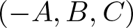
\Bigl( \alpha{\frac{\partial u}{\partial t}}+{\frac{1}{4}}{\frac{\partial^3u}{\partial z^3}}-{\frac{3}{2}}u{\frac{\partial u}{\partial z}}\Bigr)=0.\end{equation} There are many significant applications in physics and algebraic geometry, for which we refer the reader to [Reference Blower6] and [Reference Blower and Doust9]. For 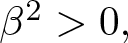 $\beta^2 \gt 0,$ we have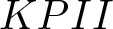 $KPII$; whereas for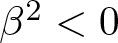 $\beta^2 \lt 0$, we have $KPI$. The existence theory is different in these two cases; see [Reference Birman and Solomjak3–Reference Blower5]. The purpose of this paper is to produce solutions as Fredholm determinants of certain families of operators. Mulase showed that $KP$ is completely integrable in the sense of Frobenius; however, his process is algebraic except for the computation of infinitely many recursive indefinite integrals [Reference Mulase50, p. 66], so does not furnish explicit solutions. See also [Reference Magnot and Reyes45].
We obtain solutions of this equation by a method associated with Gelfand, Levitan, and Marchenko (GLM), by expressing  $u$ in terms of the Fredholm determinant of a certain integral operator. As in previous papers [Reference Blower and Doust9], [Reference Blower6], [Reference Blower and Newsham13], we introduce this determinant indirectly from a family of continuous-time linear systems and related operators.
The method for solving the nonlinear evolution equation splits into a forward problem, a linear evolution, and an inverse problem.
(i) The potential $u$ is part of a linear ODE which generates spectral data, including a scattering function
$\phi$. We express
$\phi$ as the impulse response function of a linear system
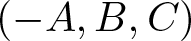
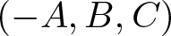
$(-A,B,C)$ with state space
$H$.
$u$ is part of a linear ODE which generates spectral data, including a scattering function
$\phi$. We express
$\phi$ as the impulse response function of a linear system
$(-A,B,C)$ with state space
$H$.(ii) The scattering data evolves according to a linear ODE, which we obtain by evolving the linear systems through a family
$(-A, B(t), C(t))$.(iii) From the
$(-A, B(t), C(t))$, we recover potentials
$u(\cdot ,t)$ from various determinant formulas, especially the Gelfand–Levitan equation (2.3). Our solution of (2.3) features a family of linear operators
$R_x$ on
$H$, which satisfy a Lyapunov equation (1.4) and algebraic identities in Propositions 4.4 and 7.2. An aspect of (i) is producing a suitable
$(-A,B,C)$ for a given
$\phi$. In Section 9, we achieve this explicitly for a class of
$\phi$ that occurs in differential equations.


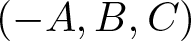





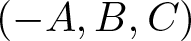


Definition Let  $H$ be a complex separable Hilbert space, which we regard as the state space, and $H_0$ a complex finite-dimensional Hilbert space, used as the input and output space. Let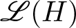 ${\mathscr{L}}(H)$ be the space of bounded linear operators on $H$ with the operator norm, which contains the space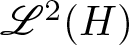 ${\mathscr{L}}^2(H)$ of Hilbert–Schmidt operators as an ideal. The ideal of trace-class operators is $\mathscr{L}^1(H)=\{\Phi\Psi: \Phi, \Psi\in \mathscr{L}^2(H)\}$. A continuous-time linear system is a triple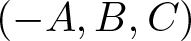 $(-A,B,C)$ where
(i)
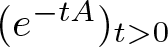
$-A$ is the generator of a strongly continuous semigroup
$(e^{-tA})_{t \gt 0}$ on
$H$, which is bounded so
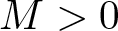
$\Vert e^{-tA}\Vert_{{\mathscr{L}}(H)}\leq M$ for some
$M \gt 0$ and all
$t \gt 0$; then the domain
${\mathscr{D}}(A)$ of
$A$ is a dense linear subspace of
$H$ which is itself a Hilbert space for the norm
$\Vert h\Vert_{{\mathscr{D}}(A)}=(\Vert h\Vert^2+\Vert Ah\Vert^2)^{1/2}$;(ii)
$B:{{H_0}}\rightarrow {\mathscr{D}}(A)$ is a bounded linear operator;(iii)
$C:{\mathscr{D}}(A)\rightarrow {{H_0}}$ is a bounded linear operator. [Alternatively, one can take
$B:{\mathbb{C}}\rightarrow H$ and
$C:H\rightarrow {\mathbb{C}}$ bounded.]










Then one defines the impulse response function  $\phi: (0, \infty)\rightarrow {\mathscr{L}}({H_0})$ by $\phi (t)=Ce^{-tA}B$, Suppose that $\int_0^\infty t\Vert\phi (t)\Vert^2_{\mathscr{L}^2(H_0)}\, dt$ converges; then the Hankel integral operator
 \begin{equation}\Gamma_\phi f(z)=\int_0^\infty \phi (z+\zeta )f(\zeta )d\zeta \qquad (f\in L^2((0, \infty ); H_0 ))\end{equation}
defines a Hilbert–Schmidt operator on  $L^2((0, \infty ); H_0).$ Then we take the family of linear systems $(-A, e^{-xA}B, e^{-xA}C)$ depending upon parameter $x \gt 0$, and consider the corresponding impulse response functions $\phi_{(x)}(t)=Ce^{-(2x+t)A}B$, and the Hankel integral operators with kernels $Ce^{-(2x+z+\zeta )A}B$. See [Reference Megretski, Peller and Treil49].
The fundamental operator in continuous-time linear systems is the right translation operator  $S_t:f(x)\mapsto f(x-t)$ on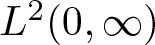 $L^2(0, \infty )$, which gives rise to a semigroup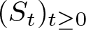 $(S_t)_{t\geq 0}$ of isometries. In Section 2, we establish the fundamental properties of the operators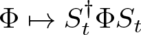 $\Phi\mapsto S_t^\dagger \Phi S_t$ and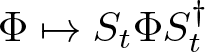 $\Phi\mapsto S_t\Phi S_t^\dagger$ on the Hilbert–Schmidt operators on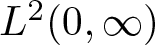 $L^2(0, \infty )$. Theorem 2.4 includes Pöppe’s fundamental identity on products of Hankel operators in terms of almost derivations on algebras of operators; see [Reference McKean48], [Reference Pöppe60, § 5] and [Reference Pöppe58]. This basic concept from Hochschild theory motivates the special tools from Pöppe’s theory, notably the bracket operation. We prefer to express similar concepts in terms of operators on the state space of the linear system.
In [Reference Blower6], we considered the family of operators
 \begin{equation}R_x=\int_x^\infty e^{-tA}BCe^{-tA}\, dt\end{equation}
on  $H$, which gives a solution of Lyapunov’s equation
 \begin{equation}{\frac{dR_x}{dx}}=-AR_x-R_xA, \quad \Bigl({\frac{dR_x}{dx}}\Bigr)_{x=0}=-BC.\end{equation}
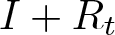
 As a consequence of this identity, the  $R_x$ have a remarkable algebraic structure which is reflected in the tau function $\tau (x)=\det (I+R_x)$. In [Reference Blower6] Propositions 2.2 and 2.3, we gave sufficient conditions for $R_x$ to be trace class. In [Reference Blower and Newsham13] we introduced a differential ring of operators on $H$, and used this to produce solutions of $KdV$. In the current paper, we introduce families of linear systems, and thereby solve $KP$.
$KP$.
There are several definitions of tau function in the literature, reflecting the diverse contexts in which they arise. Segal and Wilson showed that the common terminology is appropriate by reconciling the various notions in the common context of the  $KdV$ equation. They showed that the Baker–Akhiezer function for the $KdV$ equation may be expressed [Reference Segal and Wilson64, Proposition 5.14] in terms of the tau function as defined by the Japanese school. Our linear systems produce solutions of the Gelfand–Levitan equation that generate Baker–Akhiezer functions [Reference Blower and Newsham13, Proposition 3.2]. In [Reference Blower7], we showed that Jacobian theta functions on algebraic curves of genus one, namely elliptic curves, can be expressed as tau functions of periodic linear systems, and indicated how this notion could be extended to hyperelliptic curves of higher genus. The $KdV$ dynamical system can be integrated using hyperelliptic curves by the approach of [Reference Mumford52, 3.177]. We regard our linear system approach as work in progress, with potential extension to the case of infinite genus via the spectral curve of Hill’s equation.
The tau function generalizes the classical notion of a theta function, as follows. Mulase [Reference Mulase, Penner and Yau51, Theorem 6.1, Corollary] showed that an abelian variety defined over  ${\mathbb C}$ is the Jacobian variety of a certain algebraic curve if and only if it can be the orbit of a $KP$ dynamical system. The orbits of the $KP$ dynamical system are linear flows in the Jacobian. This is clear for one-soliton solutions, as in (10.11). Shiota [Reference Shiota65] gives a rigorous and detailed account of how $KP$ solves Schottky’s problem.
A significant case arises when 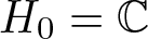 $H_0={\mathbb C}$, and much information is captured by the potential $q(x)=-2{\frac{d^2}{dx^2}} \log \tau (x)$. Gelfand and Levitan considered the Fourier transform of the spectral measure, and related this to wave equations. In this paper, we use a similar idea, except that the operators in wave equation have matrix coefficients and the operators are not necessarily self-adjoint, so there is no spectral measure in the usual sense. To obtain substitutes, we have a preliminary Section 3 which introduces relevant notions of spectrum via functional calculus for operator cosine families, as in [Reference Goldstein35].
For reasons discussed in [Reference Mumford52, 3.239],  $KP$ includes as special cases several significant partial differential equations in mathematical physics. We proceed from the simplest cases towards the general, so that the solutions are as explicit as possible. In Section 4, we obtain solutions of the Zakharov–Shabat system, and in Section 5, describe the related spectral theory. In [Reference Newell, Bullough and Caudrey53], Newell gives a detailed description of the inverse scattering transform associated with the Zakharov-Shabat and Schrödinger eigenvalue problems.
In [Reference Mumford52, 3.239], the theta functions satisfy special addition rules known as Fay’s identities which are essential to the derivations of the PDE. Whereas there are corresponding versions for operators [Reference Dupré, Glazebrook and Previato28], we have not yet identified the class of linear systems 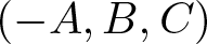 $(-A,B,C)$ such that the corresponding tau functions satisfy Fay’s identities.
In Section 6, we introduce linear systems with infinite-dimensional state spaces and formulate conditions that ensure the  $R_x$ operators are trace class, so that the necessary tau functions exist. In Section 7, we introduce the differential ring structure that is essential for solving $KP$. Equipped with this algebra, we proceed to obtain solutions for $KP$ in Section 8.
In Section 10, utilizing the linear systems approach for the  $KP$ equation we have presented herein, we implement three numerical methods for computing solutions to the $KP$ equation. The first two methods are based on numerically solving the GLM equation for given scattering data, while the third method is based on computing the $\tau$ function via the Fredholm determinant for the $KP$ equation. A fourth numerical method based on a direct exponential time-stepping pseudo-spectral scheme is also implemented for comparison purposes. The scattering data represent the solution to the linearized $KP$ equation evaluated at any time $t \gt 0$. In the case of the GLM-based methods, for any such given scattering data, we solve the linear integral GLM equation using both a Riemann Rule and Clenshaw–Curtis quadrature based on Chebyshev polynomial approximation; see Clenshaw and Curtis [Reference Clenshaw and Curtis20]. This generates an approximate solution to the $KP$ equation at that time $t \gt 0$. In the case of the $\tau$ function based method, we approximate the Fredholm determinant associated with the scattering data, using the Nyström–Clenshaw–Curtis method developed by Bornemann [Reference Bornemann15]. Indeed, Bornemann’s use of Clenshaw–Curtis quadrature to evaluate such determinants inspired our GLM approximation method using this quadrature. We implement all four numerical methods in the case of scattering data corresponding to a two-soliton interaction scenario. Such scattering data are analytic, and we observe exponential convergence in both methods based on Clenshaw–Curtis quadrature, as outlined by Bornemann [Reference Bornemann15, p. 892].
There has been much recent interest in the use of linear systems and direct linearization methods to solve integrable systems and the  $KP$ equation in particular. The approach we adopt herein is closely related to the methods developed by Pöppe, see Pöppe [Reference Pöppe58–Reference Pöppe60], Pöppe and Sattinger [Reference Pöppe and Sattinger61], Bauhardt and Pöppe [Reference Bauhardt and Pöppe1], McKean [Reference McKean48], and by Nijhoff, see Nijhoff Quispel, Van Der Linden, Capel [Reference Nijhoff, Quispel, Linden and Capel54], Nijhoff [Reference Nijhoff55], Nijhoff and Capel [Reference Nijhoff and Capel56], Fu and Nijhoff [Reference Fu and Nijhoff32–Reference Fu and Nijhoff34] and Fu [Reference Fu31]. Also see Dyson [Reference Dyson29], Santini, Ablowitz and Fokas [Reference Santini, Ablowitz and Fokas63], Mulase [Reference Mulase50, Reference Mulase, Penner and Yau51], Pelinovsky [Reference Pelinovsky57] and Kodama [Reference Kodama44]. For the development of the linear systems approach in this context and more background, see Blower [Reference Blower8], Blower and Doust [Reference Blower and Doust9] and Blower and Newsham [Reference Blower and Newsham13]. For more details on Pöppe’s approach, see Blower and Malham [Reference Blower and Malham10–Reference Blower and Malham12], as well as Doikou, Malham and Stylianidis [Reference Doikou, Malham and Stylianidis25], Malham [Reference Malham46, Reference Malham47] and Doikou, Malham, Stylianidis, and Wiese [Reference Doikou, Malham, Stylianidis and Wiese26].
The main conclusion is that Fredholm determinants and the Gelfand–Levitan equation are highly effective methods for numerical integration of  $KP$.
$KP$.
2. Pöppe’s bracket for semi-additive operators
Our method extends that of Pöppe [Reference Pöppe59], who realized that solutions of  $KP$ are given by tau functions, namely Fredholm determinants of suitable families of integral operators. Pöppe considers semi-additive operators, which one can define as families of integral operators $\Phi_{(t)}$ on $L^2((0, \infty ), {\mathbb{C}})$ that depend upon complex parameters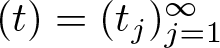 $(t)=(t_j)_{j=1}^\infty$ so that $\Phi$ has kernel $\phi (x+t_1, y +t_1; t_2, t_3, \dots )$ and
 \begin{equation}\Phi_{(t)} f(x)=\int_0^\infty \phi (x+t_1, y+t_1, t_2, \dots ) f(y)\,dy \qquad (f\in L^2((0, \infty ); {\mathbb{C}} )).\end{equation}
 In this section, we choose  $t_1=t \gt 0$, fix and suppress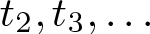 $t_2, t_3, \dots $ and regard $(x,y)$ as the primary variables.
Pöppe [Reference Pöppe59] used Fredholm determinants of semi-additive operators to solve the  $KP$ equation and additive operators to solve the $KdV$ equation. There were steps towards a universal tau function theorem that would generate solutions to PDE from the tau functions of suitable integral operators. The $\tau$ function satisfies differential equations relating to (2.3). In this section, we make the basic results precise.
Pöppe’s calculations involve certain operator formulas which reduce integral operators to finite-rank operators, and can conveniently be expressed in terminology from [Reference Cuntz and Quillen21, Section 5] or [Reference Bezrukavnikov and Kaledin2, Lemma 3.6] used to describe the Fedosov product. The origins of this idea in geometric quantization date back to Lichnérowicz. Let  $\mathscr{L}$ be a unital complex algebra with ideal $\mathscr{F}$; introduce the algebra $\mathscr{M}$ with ideal $\mathscr{J}$ by
 \begin{equation*} \mathscr{J} =\Biggl\{\begin{bmatrix} 0&f\\ 0&0\end{bmatrix} : f\in \mathscr{F}\Biggr\}\lhd \mathscr{M} =\Biggl\{\begin{bmatrix} a&b\\ 0&a\end{bmatrix} : a,b\in\mathscr{L}\Biggr\}\end{equation*}
so that 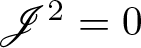 $\mathscr{J}^2=0$. Let $\pi : \mathscr{M}\rightarrow\mathscr{M}/\mathscr{J}$ be the canonical homomorphism.
Lemma 2.1. For a linear map  $\partial :\mathscr{L}\rightarrow\mathscr{L}$ with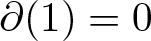 $\partial (1)=0$, the following are equivalent:
(i) the linear map
(2.2)is a homomorphism modulo\begin{equation} \rho :\mathscr{L}\rightarrow\mathscr{M}: a\mapsto \begin{bmatrix} a&\partial a\\ 0&a\end{bmatrix} \qquad (a\in \mathscr{L} )\end{equation}
$\mathscr{J}$; that is,
$\pi\circ \rho: \mathscr{L}\rightarrow \mathscr{M}/\mathscr{J}$ is a homomorphism;(ii)
$\omega :\mathscr{L}\otimes\mathscr{L}\rightarrow\mathscr{M} :$
$\omega (a,b)=\rho (ab)-\rho (a)\rho (b)$ takes values in
$\mathscr{J}$;(iii)
$\varpi :\mathscr{L}\otimes\mathscr{L}\rightarrow \mathscr{L}:$
$\varpi (a,b)=\partial (ab)-(\partial a)b-a\partial b$ takes values in
$\mathscr{F}$.









Proof. Here,  $\rho$ is linear with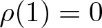 $\rho (1)=0$ by the assumptions on $\partial$. The equivalence of (i) and (ii) is clear. Also
 \begin{equation*} \omega (a,b)=\begin{bmatrix} 0&\varpi (a,b)\\ 0&0\end{bmatrix}\end{equation*}
so (ii) and (iii) are equivalent. Whereas  $\partial: \mathscr{L}\rightarrow\mathscr{L}$ is not necessarily a derivation, here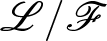 $\mathscr{L}/\mathscr{F}$ is a $\mathscr{L}$-bimodule and $\mathscr{L}\rightarrow \mathscr{L}/\mathscr{F} :$ $a\mapsto \partial (a)+\mathscr{F}$ is a derivation.
Let 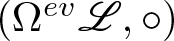 $(\Omega^{ev}\mathscr{L} , \circ)$ be the space of noncommutative differential forms on $\mathscr{L}$ that have even order, which forms an algebra for Fedosov’s product $a\circ b=ab-dadb$; for a detailed discussion, see [Reference Cuntz and Quillen21]. The following statements should be self-explanatory, with indexing to match [Reference Cuntz and Quillen22, (15)].
Proposition 2.2. Suppose that  $\partial$ satisfies the conditions of Lemma 2.1, and let $\tau :\mathscr{F}\rightarrow {\mathbb C}$ be a linear functional.
(i) Then there exists a trilinear map
\begin{equation*} \varphi_2(a_0,a_1,a_2)=\varphi_2(a_0da_1da_2)=\tau \bigl(a_0\varpi (a_1,a_2)\bigr)\qquad (a_0, a_1, a_2\in\mathscr{L}).\end{equation*}(ii) Suppose further that
$\partial$ takes values in
$\mathscr{F}$. Then
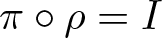
$\pi\circ\rho =I$ on
$\mathscr{L}$ and there is a linear functional
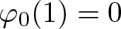
$\varphi_0 :\mathscr{L}\rightarrow {\mathbb C}$ with
$\varphi_0 (1)=0$, given by
\begin{equation*}\varphi_0(a_0)=\tau (\partial a_0)\qquad (a_0\in\mathscr{L} ).\end{equation*}





Proof. (i) Given a linear map  $\rho :\mathscr{L}\rightarrow\mathscr{M}$ with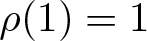 $\rho (1)=1$, there exists a unique homomorphism $\rho_*:\Omega^{ev}\mathscr{L}\rightarrow \mathscr{M}$ such that $\rho_*(a)=\rho(a)$ for all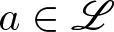 $a\in\mathscr{L}$ by the universal property of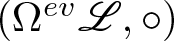 $(\Omega^{ev}\mathscr{L}, \circ )$; see [Reference Cuntz and Quillen22, Proposition 5.1] and [Reference Cuntz and Quillen21, Proposition 2.1]. For $\rho$ as in (2.2), the matrix expression for $\rho (a_0)\omega (a_1,a_2)$ is zero except for the entry in the top-right corner $a_0\varpi (a_1,a_2)\in \mathscr{F}$, to which we apply $\tau$.
(ii) When  $\partial$ takes values in $\mathscr{F}$, the conditions of Lemma 2.1(iii) are obviously satisfied, and we can define $\varphi_0(a_0)=\tau (\partial a_0).$
Proposition 2.2(i) applies in Theorem 2.4(iii). Clearly,  $\partial :\mathscr{L}\rightarrow\mathscr{L}$ is a derivation if and only if $\rho$ is an algebra homomorphism, as in Theorem 2.4(i). Also,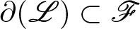 $\partial (\mathscr{L} )\subset \mathscr{F} $ if and only if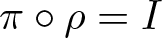 $\pi\circ\rho =I$; this situation may be compared with Theorem 2.4(iv).
(i) Let
$\mathscr{L}^2(L^2((0,\infty );{\mathbb C}))$ be the space of Hilbert–Schmidt integral operators on
$L^2((0, \infty );{\mathbb C} )$, and
$\mathscr{F}$ the ideal of finite-rank operators on
$L^2((0, \infty ); {\mathbb C})$.(ii) Suppose that
$P\in \mathscr{L}^2(L^2(0, \infty ); {\mathbb C} )$ has kernel
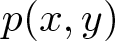
$p(x,y)$. We define the Pöppe bracket by
$[P]_{x,y} =p(x,y)$ for
$x,y\in (0, \infty )$.(iii) Let
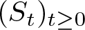
$(S_t)_{t\geq 0}$ be the strongly continuous one-parameter semigroup of isometric shift operators on
$L^2((0, \infty ); {\mathbb C} )$ given by
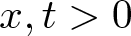
$S_tf(x)=f(x-t) {\mathbb I}_{(0, \infty )}(x-t)$ for
$x,t \gt 0$ and
$f\in L^2((0, \infty ); {\mathbb C} )$, otherwise known as the right-translation operators.










The following includes the fundamental identities of Pöppe in terms of translation semigroups; see [Reference Pöppe60, p. 622].
(i) Let
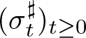
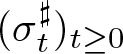
$\sigma_t^\sharp (\Phi )=S_t\Phi S_t^\dagger.$ The
$(\sigma^\sharp_t)_{t\geq 0}$ gives a strongly continuous one-parameter semigroup of isometric algebra homomorphisms on
$\mathscr{L}^2(L^2((0,\infty );{\mathbb C}))$; the infinitesimal generator
$\partial^\sharp$ of
$(\sigma_t^\sharp )_{t\geq 0}$ is a derivation and its domain is an algebra.(ii) Let
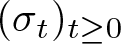
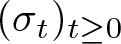
$\sigma_t (\Phi )=S_t^\dagger \Phi S_t.$ Then
$(\sigma_t)_{t\geq 0}$ gives a strongly continuous one-parameter semigroup of contractions on
$\mathscr{L}^2(L^2((0,\infty );{\mathbb C}))$ which preserves the upper-triangular form of the GLM equation
(2.3)\begin{equation} \phi (x,y)+T(x,y) +\int_x^\infty T(x,z)\phi (z,y)\, dz=0\qquad (0 \lt x \lt y).\end{equation}(iii) Let
$\partial $ be the infinitesimal generator of the semigroup
$(\sigma_t)_{t\geq 0}$ and let
$\Phi, \Psi$ and
$\Phi\Psi$ belong to the domain of
$\partial$. Then the cocycle
(2.4)satisfies\begin{equation}\varpi (\Phi ,\Psi )=\partial (\Phi\Psi) -(\partial\Phi )\Psi -\Phi (\partial\Psi)\end{equation}(2.5)\begin{equation}\bigl[\Upsilon\varpi (\Phi ,\Psi )\Lambda\bigr]_{x,y}=[\Upsilon\Phi ]_{x,0}[\Psi \Lambda]_{0,y}\qquad (\Upsilon, \Lambda\in \mathscr{L}^2((L^2(0,\infty ); {\mathbb C} ))).\end{equation}(iv) Let
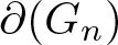
$G_n=\Gamma_{\phi_1}\dots \Gamma_{\phi_{2n}}$ be a product of an even number of Hankel operators. Then
$\partial(G_n)$ has finite rank.










Proof. (i) The standard inner product on  $\mathscr{L}^2(L^2((0,\infty );{\mathbb C}))$ is $\langle \Phi ,\Psi \rangle =\mathop{\mathrm{trace}} (\Phi \Psi^\dagger )$, and one easily checks that $\langle \sigma_t(\Phi ), \Psi\rangle =\langle \Phi , \sigma_t^\sharp \Psi \rangle$. In Proposition 1 of [Reference Blower and Malham10], we established that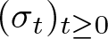 $(\sigma_t)_{t\geq 0}$ is a strongly continuous contraction semigroup, and the corresponding properties of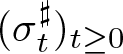 $(\sigma_t^\sharp )_{t\geq 0}$ are obtained by passing to the adjoint semigroup and invoking [Reference Davies23, Theorem 6.18]. Each $\sigma_t^\sharp$ is an isometry since we have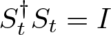 $S_t^\dagger S_t=I$, hence,
 \begin{equation*}\langle\sigma_t^\sharp \Phi , \sigma_t^\sharp\Phi\rangle=\mathop{\mathrm{trace}} ( S_t\Phi S_t^\dagger (S_t\Phi S_t^\dagger )^\dagger) =\mathop{\mathrm{trace}} (S_t\Phi \Phi^\dagger S_t^\dagger )=\mathop{\mathrm{trace}} (S_t^\dagger S_t\Phi\Phi^\dagger )=\langle\Phi ,\Phi\rangle.\end{equation*}
 Likewise,  $\sigma_t^\sharp$ is an algebra homomorphism since
 \begin{equation}\sigma_t^\sharp (\Phi\Psi)=S_t\Phi\Psi S_t^\dagger=S_t\Phi S_t^\dagger S_t\Psi S_t^\dagger =\sigma_t^\sharp (\Phi )\sigma_t^\sharp (\Psi ).\end{equation}
 We introduce  $\mathscr{A}_0=\{aI+ \Phi: a\in {\mathbb C} , \Phi\in\mathscr{L}^2(L^2((0,\infty );{\mathbb C}))$, which is a Banach algebra with norm $\Vert aI+\Phi\Vert =\vert a\vert+ \Vert\Phi\Vert_{\mathscr{L}^2}$ on which $aI+\Phi \mapsto aI+S_t\Phi S_t^\dagger$ gives a strongly continuous semigroup, extending $\sigma_t^\sharp$. Then by differentiating (2.6) at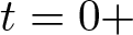 $t=0+$, we find $\partial^\sharp (\Phi\Psi )=(\partial^\sharp\Phi)\Psi +\Phi \partial^\sharp \Psi$ on the algebra
 \begin{equation}\mathscr{D} (\partial^\sharp )=\bigl\{aI+\Phi: a\in{\mathbb C} ;\Phi, \partial^\sharp\Phi\in\mathscr{L}^2(L^2((0,\infty );{\mathbb C} ))\bigr\}.\end{equation}
 (ii) In Proposition 1 of [Reference Blower and Malham10], we established the analytical properties of 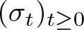 $(\sigma_t)_{t\geq 0}$. It is straightforward to show that if $\Phi$ is a Hilbert–Schmidt integral operator with kernel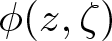 $\phi (z, \zeta )$, then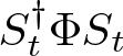 $S_t^\dagger \Phi S_t$ is the integral operator that has kernel $\phi (z+t, \zeta +t)$. Also $\mathscr{L}=\{aI+\Phi: a\in {\mathbb C} , \Phi\in \mathscr{L}^2\}$ is an algebra on which $\sigma_t$ operates, and $\mathscr{L}$ contains the ideal $\mathscr{F}$ of finite rank operators. The simple substitution $(x,y)\mapsto (x+t,y+t)$ preserves the form of equation (2.3).
(iii) The Hochschild cocycle relation
 \begin{equation} \Upsilon\varpi (\Phi ,\Psi )-\varpi (\Upsilon\Phi ,\Psi )+\varpi (\Upsilon, \Phi \Psi )-\varpi (\Upsilon ,\Phi )\Psi =0\end{equation}
is a direct consequence of the definition of  $\varpi$.
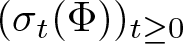
Let  $\Phi, \Psi\in\mathscr{L}^2(L^2((0,\infty );{\mathbb C}))$, and let $P=\Phi\Psi$ have kernel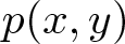 $p(x,y)$ so $\sigma_t(P)$ has kernel $p(x+t, y+t)$ where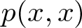 $p(x,x)$ determines an element of $L^1((0, \infty ); {\mathbb C})$. Then by Lebesgue’s differentiation theorem, $h^{-1}\int_0^h \vert p(x+t,x+t)-p(x,x)\vert dt\rightarrow 0$ as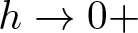 $h\rightarrow 0+$, for almost all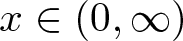 $x\in (0, \infty )$. Also, observe that $P$ determines a trace-class operator. We have $[P]_{x,x}=[\sigma_x(P)]_{0,0}$, hence, $(d/dx)[P]_{x,x}=[\partial\sigma_x(P)]_{0,0}$. In Proposition 7.2, we provide another expression for this diagonal derivative.
In contrast to the situation of (i)  $\sigma_t$ is not an algebra homomorphism for $t \gt 0$ since $S_tS_t^\dagger$ corresponds to multiplication by ${\mathbb I}_{[t, \infty )}$, and $\partial$ is not a derivation in $\mathscr{L}^2$; however, $\partial $ is a derivation modulo the finite-rank operators. Indeed, the discrepancy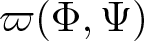 $\varpi (\Phi ,\Psi )$ is given by the integral operator with kernel
 \begin{align}\int_0^\infty \Bigl({\frac{\partial\phi}{\partial x}}(x,z)\psi (z,y)& +\phi (x,z){\frac{\partial \psi }{\partial y}} (z,y)\Bigr) dz-\int_0^\infty \Bigl({\frac{\partial\phi}{\partial x}}(x,z)+{\frac{\partial \phi }{\partial z}}(x,z)\Bigr)\psi (z,y)\, dz\nonumber\\
&-\int_0^\infty \phi (x,z)\Bigl({\frac{\partial\psi}{\partial z}}(z,y)\psi (z,y) +{\frac{\partial \psi }{\partial y}} (z,y)\Bigr) dz\nonumber\\
&=-\int_0^\infty \Bigl( {\frac{\partial \phi }{\partial z}}(x,z)\psi (z,y)+\phi (x,z){\frac{\partial\psi}{\partial z}}(z,y)\psi (z,y)\Bigr) dz\nonumber\\
&=\phi (x,0)\psi (0,y).\end{align}
\begin{align}\int_0^\infty \Bigl({\frac{\partial\phi}{\partial x}}(x,z)\psi (z,y)& +\phi (x,z){\frac{\partial \psi }{\partial y}} (z,y)\Bigr) dz-\int_0^\infty \Bigl({\frac{\partial\phi}{\partial x}}(x,z)+{\frac{\partial \phi }{\partial z}}(x,z)\Bigr)\psi (z,y)\, dz\nonumber\\
&-\int_0^\infty \phi (x,z)\Bigl({\frac{\partial\psi}{\partial z}}(z,y)\psi (z,y) +{\frac{\partial \psi }{\partial y}} (z,y)\Bigr) dz\nonumber\\
&=-\int_0^\infty \Bigl( {\frac{\partial \phi }{\partial z}}(x,z)\psi (z,y)+\phi (x,z){\frac{\partial\psi}{\partial z}}(z,y)\psi (z,y)\Bigr) dz\nonumber\\
&=\phi (x,0)\psi (0,y).\end{align} The result follows when we apply  $\Upsilon $ on the left and $\Lambda$ on the right. Compare [Reference Blower and Malham10, Lemma 1] and [Reference Pöppe60, § 5].
(iv) The proof is by induction on  $n$. For $n=1$, we observe that $G_1=\Gamma_{\phi_1}\Gamma_{\phi_2}$ gives $\partial G_1$ which has kernel $-\phi_1(x)\phi_2(x)$. Then $G_{n+1}=G_n(\Gamma_{\phi_{2n-1}}\Gamma_{\phi_{2n}})$ gives
 \begin{align}\partial G_{n+1}=&\big( \partial (G_n(\Gamma_{\phi_{2n-1}}\Gamma_{\phi_{2n}}))-
(\partial G_n)(\Gamma_{\phi_{2n-1}}\Gamma_{\phi_{2n}})-G_n\partial (\Gamma_{\phi_{2n-1}}\Gamma_{\phi_{2n}})\nonumber\\
&\quad +\partial( G_n)(\Gamma_{\phi_{2n-1}}\Gamma_{\phi_{2n}})+G_n\partial (\Gamma_{\phi_{2n-1}}\Gamma_{\phi_{2n}})\end{align}
\begin{align}\partial G_{n+1}=&\big( \partial (G_n(\Gamma_{\phi_{2n-1}}\Gamma_{\phi_{2n}}))-
(\partial G_n)(\Gamma_{\phi_{2n-1}}\Gamma_{\phi_{2n}})-G_n\partial (\Gamma_{\phi_{2n-1}}\Gamma_{\phi_{2n}})\nonumber\\
&\quad +\partial( G_n)(\Gamma_{\phi_{2n-1}}\Gamma_{\phi_{2n}})+G_n\partial (\Gamma_{\phi_{2n-1}}\Gamma_{\phi_{2n}})\end{align}where the first term on the right-hand side is in  $\mathscr{F}$ by (2.4) and (2.9), while the final two terms are in $\mathscr{F}$ by the induction hypothesis. See also [Reference McKean48, Section 3.5].
Example 2.5. (i) In [Reference Blower and Malham10, Proposition 1(vi)], we identified  $\varphi_0(\Phi )=\mathop{\mathrm{trace}} (\partial\Phi )=-[\Phi ]_{0,0}$.
(ii) In the context of Theorem 2.4(i) and (iv), let  $\Phi\in \mathscr{L}^2((0, \infty ); {\mathbb C}))$ have kernel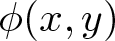 $\phi (x,y)$, and let $\Psi=\Gamma_{\psi_1}\Gamma_{\psi_2}$ be a product of Hankel operators, such that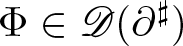 $\Phi\in \mathscr{D}(\partial^\sharp )$. Then the usual trace formula on $\mathscr{L}^2((0, \infty ); {\mathbb C})$ gives
 \begin{equation*} \mathop{\mathrm{trace}}\bigl( \Phi\partial^\sharp \Psi \bigr)=\int_0^\infty\int_0^\infty \phi (x,y)\psi_1(y)\psi_2(x)\, dxdy.\end{equation*}
Remark 2.6. The natural development of Theorem 2.4(i) follows the route of [Reference Cuntz and Quillen22, Section 12]. Let  $\mathscr{D}$ be a complex unital algebra, let $\mathscr{M}$ be an $\mathscr{D}$-bimodule, and $V$ a complex vector space. Let the commutator subspace of $\mathscr{M}$ be $[M, \mathscr{D}] =\mathop{\mathrm{span}}\{am-ma: a\in\mathscr{D}, m\in\mathscr{M}\}$. A trace $\tau: \mathscr{M}\rightarrow V$ is a linear map $\tau:\mathscr{M}\rightarrow V$ such that $\tau\vert [\mathscr{M}, \mathscr{D}]=0$. Given a derivation $\partial^\sharp: \mathscr{D}\rightarrow \mathscr{M}$, there exists an $\mathscr{D}$-bimodule map $\Omega^1\mathscr{D}\rightarrow \mathscr{M}$ such that $\Phi d\Psi\mapsto \Phi \partial^\sharp\Psi$; thus, a trace $\tau:\mathscr{M}\rightarrow V$ gives a trace $\varphi :\Omega^1\mathscr{A}\rightarrow V:$ $\varphi (\Phi d\Psi)=\tau (\Phi\partial^\sharp \Psi).$
Next we form matrices with entries in these spaces and extend the algebraic structures in the natural way. We can amplify  $\varphi$ to $\varphi_n:M_{n\times n}(\Omega^1\mathscr{D} )\rightarrow V$ by $\varphi_n(A\otimes \Phi d\Psi)=\mathop{\mathrm{trace}} (A)\varphi (\Phi d\Psi )$, where $\mathop{\mathrm{trace}} :M_{n\times n}({\mathbb C})\rightarrow {\mathbb C}$ is the usual trace. Then we let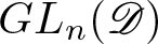 $GL_n(\mathscr{D})$ be the multiplicative group consisting of invertible elements of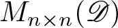 $M_{n\times n}(\mathscr{D} )$. Writing $\{A,B\}=ABA^{-1}B^{-1}$ for the multiplicative commutator, we can introduce the normal subgroup $\{GL_n(\mathscr{D}), GL_n(\mathscr{D})\}$ that is generated by the multiplicative commutators. Using the trace property of $\tau$ repeatedly, we find
 \begin{equation*} \varphi_n \bigl((\Phi\Psi)^{-1}d(\Phi \Psi )\bigr)=\varphi_n (\Phi^{-1}d\Phi)+\varphi_n (\Psi^{-1}d\Psi ),\end{equation*}
and
 \begin{equation*} \varphi_n \bigl(\{\Phi , \Psi \}^{-1}d\{\Phi , \Psi \}\bigr)= 0\qquad (\Phi, \Psi\in GL_n(\mathscr{D})).\end{equation*}
 Hence,  $\Phi\mapsto \varphi (\Phi^{-1}d\Phi )$ induces a group homomorphism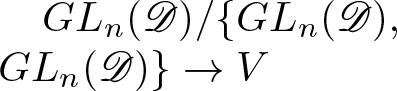 $GL_n(\mathscr{D}) /\{GL_n(\mathscr{D} ),\\ GL_n(\mathscr{D} )\}\rightarrow V$. There are numerous closely related determinant and trace formulas involving this idea, as discussed in [Reference Böttcher, Widon and Jacobi17],
(i) A semi-additive kernel is the family of kernels from the orbit
$(\sigma_t(\Phi ) )_{t\geq 0}$ of some
$\Phi\in \mathscr{L}^2(L^2((0, \infty ); {\mathbb C}))$.(ii) The tau function of a trace-class kernel
$P$ is
$\tau (x)=\det (I+\sigma_x(P)).$



Suppose that  $\psi \in L^2 ((0, \infty ); H')$ and $\xi \in L^2 ((0, \infty );H)$, and $\phi (z, \zeta )=\psi (z)\xi (\zeta )$. Then with $R_x=\int_x^\infty \xi (z)\psi (z)dz$, we have a family of bounded linear operators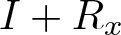 $I+R_x$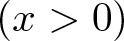 $(x \gt 0)$ on $H$ which are invertible for all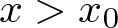 $x \gt x_0$ for some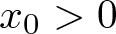 $x_0 \gt 0$. Then we can introduce a kernel
 \begin{equation*} T(x,y)=-\psi (x)\bigl( I+R_x)^{-1}\xi (y) \qquad (x_0 \lt x \lt y).\end{equation*}
Lemma 2.8. Then (2.3) holds and
 \begin{equation*} T(x,x)={\frac{d}{dx}}\log \tau (x)\qquad (x \gt x_0).\end{equation*}
Proof. The GLM equation follows by a direct substitution. Then
 \begin{align}{\frac{d}{dx}}\log\det (I+R_x)&={\hbox{trace}}\Bigl( (I+R_x)^{-1}{\frac{dR_x}{dx}}\Bigr)\nonumber\\
&=-\mathop{\mathrm{trace}}\Bigl( (I+R_x)^{-1}\xi (x)\psi (x)\Bigr)\nonumber\\
&=-\psi (x)(I+R_x)^{-1}\xi (x)\nonumber\\
&=T(x,x).\end{align}
\begin{align}{\frac{d}{dx}}\log\det (I+R_x)&={\hbox{trace}}\Bigl( (I+R_x)^{-1}{\frac{dR_x}{dx}}\Bigr)\nonumber\\
&=-\mathop{\mathrm{trace}}\Bigl( (I+R_x)^{-1}\xi (x)\psi (x)\Bigr)\nonumber\\
&=-\psi (x)(I+R_x)^{-1}\xi (x)\nonumber\\
&=T(x,x).\end{align} In previous papers [Reference Blower6], [Reference Blower and Newsham13], we have developed Pöppe’s approach, starting from linear systems and forming differential rings. In Definition 4.9 and Proposition 7.1, we introduce another bracket operation which facilitates calculation of 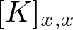 $[K]_{x,x}$ and its derivatives, so we can compute $\tau$. Our results on differential rings are equivalent in some cases to Pöppe’s results on semi-additive operators, although we regard our approach as more natural, more closely aligned with algebraic formalism that is used in differential Galois theory and elsewhere, and less dependent on isolated ingenious identities.
By [Reference Blower6, Lemma 5.1], the solution 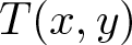 $T(x,y)$ to (2.3) satisfies
 \begin{equation}{\frac{\partial^2T}{\partial y^2}}-{\frac{\partial^2 T}{\partial x^2}}=2\Bigl({\frac{dT}{dx}}(x,x)\Bigr) T(x,y)\qquad (0 \lt x \lt y)\end{equation}
which is a wave equation, albeit with a potential 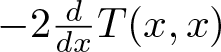 $-2{\frac{d}{dx}}T(x,x)$ that is typically a matrix, not necessarily self-adjoint. In the next Section 3, we develop a functional calculus for this context.
3. Spectra of linear systems
Let  $q\in C_b([0, \infty );{\mathbb R} )$ with $\int_0^\infty x\vert q(x)\vert dx \lt \infty$ and consider the differential operator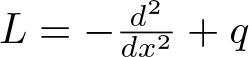 $L=-{\frac{d^2}{dx^2}}+q$, which is self-adjoint for suitable boundary conditions. Hence, for $f\in L^2(0, \infty );{\mathbb C} )$, we can define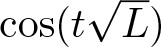 $\cos (t\sqrt{L})$ so that $u(t,x)=\cos (t\sqrt{L})f(x)$ satisfies the wave equation
 \begin{align}
{\frac{\partial^2}{\partial t^2}}u(x,t)&-{\frac{\partial^2}{\partial x^2}}u(t,x)+q(x)u(t,x)=0;\nonumber
\\u(0,x)&=f(x);\nonumber\\
{\frac{\partial u(0,x)}{\partial t}}&=0.
\end{align}
\begin{align}
{\frac{\partial^2}{\partial t^2}}u(x,t)&-{\frac{\partial^2}{\partial x^2}}u(t,x)+q(x)u(t,x)=0;\nonumber
\\u(0,x)&=f(x);\nonumber\\
{\frac{\partial u(0,x)}{\partial t}}&=0.
\end{align} Gelfand and Levitan used this as the foundation of their spectral theory of second-order differential operators. In the current paper, we make a modest extension of their theory to deal with potential  $q$ that are not necessarily real, so $L$ is not necessarily self-adjoint, but the wave equation is still useful. In Example 3.7, we consider examples of differential equations which in Section 4 we analyse in terms of linear systems.
We review some notions of spectral theory.
Definition 3.1. For a closed operator  $\Delta$ with dense domain $\mathscr{D} (\Delta )$ in Hilbert space $H$, let $\rho (\Delta )$ be the resolvent $\rho (\Delta )= \{\lambda \in {\mathbb C}: \exists (\lambda I-\Delta )^{-1}\in \mathscr{L} (H)\}$ and let the spectrum be $\sigma (\Delta )={\mathbb C}\setminus \rho (\Delta )$, a change to the notation from Section 2. The spectral bound $s(\Delta )=\sup\{\mathop{{\rm Re}} \lambda : \lambda\in \sigma (\Delta )\}$. Then the approximate point spectrum is
 \begin{equation*}\sigma_{ap} (\Delta )= \{\lambda \in {\mathbb C} : (\lambda I-\Delta )\mathscr{D} (\Delta )\, \hbox{not closed}\}\cup
\{\lambda \in {\mathbb C} : \lambda I-\Delta\, {\hbox{not injective}}\},
\end{equation*}
\begin{equation*}\sigma_{ap} (\Delta )= \{\lambda \in {\mathbb C} : (\lambda I-\Delta )\mathscr{D} (\Delta )\, \hbox{not closed}\}\cup
\{\lambda \in {\mathbb C} : \lambda I-\Delta\, {\hbox{not injective}}\},
\end{equation*}where the final set gives the point spectrum, namely the set of eigenvalues.
Consider the operator
 \begin{equation} \Delta=\begin{bmatrix} 0&I\\ -L_1&0\end{bmatrix}\qquad \begin{matrix} H^1\\ L^2\end{matrix}\end{equation}
and suppose that  $\Delta$ generates a strongly continuous semigroup $e^{t\Delta}$ such that $\Vert e^{t\Delta}\Vert \leq Me^{\omega_0t}$ for all $t\geq 0$. Then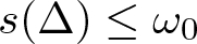 $s(\Delta )\leq \omega_0$. The topological boundary of $\sigma (\Delta )$ and the approximate point spectrum of $\Delta$ are related by $\partial \sigma (\Delta )\subseteq \sigma_{ap} (\Delta )$, and $e^{t\sigma_{ap}(\Delta )}\subseteq \sigma_{ap} (e^{t\Delta })$ for all $t\geq 0$. We defer discussion of the point spectrum until Proposition 3.6.
Let  $\mathscr{R}_0$ the subalgebra of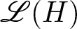 $\mathscr{L} (H)$ that generated by the set of $r(\Delta )$, where $r$ is a complex proper rational function which is holomorphic on $\sigma (\Delta )$, and let $\mathscr{R}$ be the norm closure of $\mathscr{R}_0$ in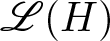 $\mathscr{L} (H)$. Given a complex and commutative Banach algebra $\mathscr{A}$ and a homomorphism $\theta:\mathscr{A}\rightarrow \mathscr{R}$, there is an induced map $\mathop{\mathrm{spec}} m(\mathscr{R})\rightarrow \mathop{\mathrm{spec}} m(\cal A)$ between the corresponding maximal ideal spaces given by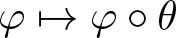 $\varphi\mapsto \varphi\circ \theta$ for every multiplicative linear functional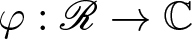 $\varphi :\mathscr{R}\rightarrow{\mathbb C}$ that corresponds to a maximal ideal of $\mathscr{R}$. A useful choice of $\mathscr{A}$ is obtained from cosine families.
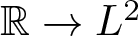
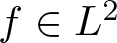
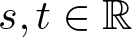
Definition 3.2. A cosine family on  $L^2$ is a family $(\mathop{\mathrm{Cos}} (t))_{t\in {\mathbb R}}\subset \mathscr{L} (L^2)$ such that
(i)
$t\mapsto \mathop{\mathrm{Cos}} (t)f$ is continuous
${\mathbb R} \rightarrow L^2$ for all
$f\in L^2$;(ii)
$\mathop{\mathrm{Cos}} (s+t)+\mathop{\mathrm{Cos}} (s-t)=2\mathop{\mathrm{Cos}} (s)\mathop{\mathrm{Cos}} (t)$ for all
$s,t\in {\mathbb R}$;(iii)
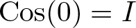
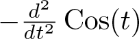
$\mathop{\mathrm{Cos}} (0)=I$, and the generator is
$-{\frac{d^2}{dt^2}}\mathop{\mathrm{Cos}} (t)$; see [Reference Goldstein35].


We have two cases to consider for  $\Delta$ and $\omega_0$ as in (3.2). First, suppose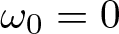 $\omega_0=0$, so the cosine family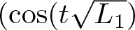 $(\cos (t\sqrt{L_1})$ is uniformly bounded on $L^2$. Then there exist an invertible $U\in {\mathscr{L}}(L^2, H)$ and a self-adjoint and non-negative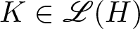 $K\in \mathscr{L}(H)$ such that $\cos (t\sqrt{L_1})=U\cos (t\sqrt {K})U^{-1}$, and in particular $\sigma (L)=\sigma (K)\subseteq [0, \infty )$.
Now consider 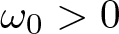 $\omega_0 \gt 0$. For $\omega \gt \omega_0 \gt 0$, we introduce the horizontal strip $\mathscr{S}_{\omega}=\{\lambda\in {\mathbb C} :\vert \mathop{{\rm Im}} \lambda \vert \lt \omega\}$ with closure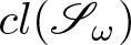 $cl(\mathscr{S}_\omega )$.
Lemma 3.3. For 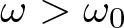 $\omega \gt \omega_0$, let $\mathscr{A}_\omega$ be the algebra of continuous functions $f: cl( \mathscr{S}_\omega )\rightarrow {\mathbb C}$ such that $f$ is holomorphic on $\mathscr{S}_\omega$, such that $f(z)=f(-z)$ and $f(z)=O(1/z^2)$ as $z\rightarrow\infty$ for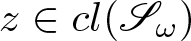 $z\in cl(\mathscr{S}_{\omega})$.
(i) Then
$\mathscr{A}_\omega$ is a Banach algebra for the norm
$\Vert f\Vert_{(\omega )}=\sup_{s\in cl(\mathscr{S}_\omega)} (1+\vert z\vert^2)\vert f(z)\vert$.(ii) There is a bounded homomorphism
$\mathscr{A}_\omega\rightarrow\mathscr{L} (L^2)$ defined by
(3.3)\begin{equation} f(\sqrt{L_1})=\int_{-\infty}^\infty \hat f(k)\cos (k\sqrt{L_1})\, {\frac{dk}{2\pi}}.\end{equation}(iii) For
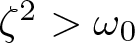
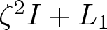
$\zeta^2 \gt \omega_0$, the operator
$\zeta^2I+L_1$ is invertible with
\begin{equation*} \zeta (\zeta^2I+L_1)^{-1}\Psi_0(x)=\int_0^\infty e^{-\zeta t}\cos (t\sqrt{L_1})\Psi_0(x)\, dt\qquad (\zeta \gt \sqrt {\omega_0}).\end{equation*}





Proof. (i) One checks that  $\Vert fg\Vert_{(\omega )}\leq \Vert f\Vert_{(\omega )}\Vert g\Vert_{(\omega )}$. Completeness of $\mathscr{A}_\omega$ follows from Morera’s theorem.
(ii) Here, we have 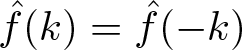 $\hat f(k)=\hat f(-k)$. Using Cauchy’s theorem, one can show that
 \begin{equation*} \hat f(k)=\int_{-\infty}^\infty f(x)e^{-ikx}\, dx=e^{-k\omega} \int_{-\infty}^\infty f(x-i\omega )e^{-ikx}\, dx\end{equation*}
so there exists 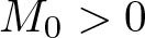 $M_0 \gt 0$ such that $\vert\hat f(k)\vert\leq M_0e^{-\omega k}$ for $k \gt 0$, so the integral (3.3) converges. Then one checks that the map $f\mapsto f(\sqrt{L_1})$ is multiplicative.
(iii) The function  $f(z)=\zeta /(\zeta^2+z^2)$ is an element of $\mathscr{A}_\omega$.
Remark 3.4. We are led to consider functions that are holomorphic on a strip due to the following example from [Reference Bloom and Heyer4, page 239]. Consider
 \begin{equation*} \varphi_\lambda (x)={\frac{\cos \lambda x}{\cosh x}}\qquad (x\in ([0, \infty ); \lambda \in \mathscr{S}_1)\end{equation*}
so that 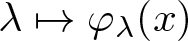 $\lambda\mapsto \varphi_\lambda (x)$ is holomorphic in $\mathscr{S}_1$, and $\vert\varphi_\lambda (x)\vert\leq 1.$ Given $f\in L^1( (0, \infty ); \cosh^2x\, dx; {\mathbb C} )$, we introduce
 \begin{equation*} \hat f(\lambda )=\int_0^\infty f(x)\varphi_\lambda (x)\cosh^2x\, dx\qquad (\lambda\in \mathscr{S}_1),\end{equation*}
and observe that  $\hat f(\lambda )$ is holomorphic on $\mathscr{S}_1$. With
 \begin{equation*} Mf(x)=-{\frac{d^2f}{dx^2}}-2\tanh x{\frac{df}{dx}}-f(x)\end{equation*}
we find that 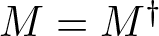 $M=M^\dagger$ in $L^2 ((0,\infty ); \cosh^2x\, dx; {\mathbb C} )$ with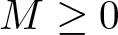 $M\geq 0$ and $M\varphi_\lambda =\lambda^2\varphi_\lambda$ for all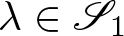 $\lambda\in \mathscr{S}_1$. There is a cosine family $(\cos (t\sqrt{M}))_{t\in{\mathbb R}}$, and the Kunze–Stein phenomenon [Reference Bloom and Heyer4, p. 124] applies to the operators
 \begin{equation*} T_Mf=\int_0^\infty f(t)\cos (t\sqrt{M})\, dt.\end{equation*}
 For 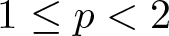 $1\leq p \lt 2$ and $f\in L^p([0, \infty ); \cosh^2 x\, dx; {\mathbb C} )$, the function $\hat f(\lambda )$ is holomorphic on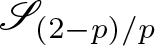 $\mathscr{S}_{(2-p)/p}$.
Let  $L_0$ be the self-adjoint differential operator which is densely defined in $H$ with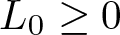 $L_0\geq 0$. Then we consider the Cauchy problem for the symmetric hyperbolic system
 \begin{equation} \begin{bmatrix} 0&-I\\ I&0\end{bmatrix} {\frac{d}{dt}} \begin{bmatrix} \psi \\ \phi \end{bmatrix} = \begin{bmatrix} L_0&0\\ 0&I\end{bmatrix} \begin{bmatrix} \psi \\ \phi \end{bmatrix}\end{equation}
with initial condition
 \begin{equation} \begin{bmatrix} \psi \\ \phi \end{bmatrix}_{t=0}=\begin{bmatrix} f\\ g\end{bmatrix}\qquad (g\in L^2((0, \infty ); \mathbb{C}), f\in H^1((0, \infty ); \mathbb{C}))\end{equation}
Then there exists a unique solution
 \begin{equation} \begin{bmatrix} \psi \\ \phi \end{bmatrix}= \begin{bmatrix} \cos t\sqrt{L_0}& {\frac{\sin t\sqrt{L_0}}{\sqrt{L_0}}}\\
-\sqrt{L_0}\sin t\sqrt{L_0}& \cos t\sqrt{L_0}\end{bmatrix}
\begin{bmatrix} f\\ g\end{bmatrix}.\end{equation}
\begin{equation} \begin{bmatrix} \psi \\ \phi \end{bmatrix}= \begin{bmatrix} \cos t\sqrt{L_0}& {\frac{\sin t\sqrt{L_0}}{\sqrt{L_0}}}\\
-\sqrt{L_0}\sin t\sqrt{L_0}& \cos t\sqrt{L_0}\end{bmatrix}
\begin{bmatrix} f\\ g\end{bmatrix}.\end{equation} To determine the eigenvalues of 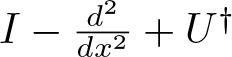 $I-{\frac{d^2}{dx^2}}+U^\dagger$, it is convenient to work with its inverse operator. In Proposition 3.6, we obtain a criterion for eigenvalues involving Pincus’s principal function [Reference Carey and Pincus19], which requires the following Lemma.
Lemma 3.5. Suppose that  $U\in L^\infty ({\mathbb R}; M_{n_0\times n_0}({\mathbb C} ))$ has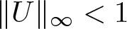 $\Vert U\Vert_\infty \lt 1$ and $U^\dagger -U=V_1V_2$ where
 \begin{equation*}V_1,V_2\in C_b^2({\mathbb R} ;M_{n_0\times n_0}({\mathbb C} ))\cap L^2({\mathbb R} ;M_{n_0\times n_0}({\mathbb C} )).\end{equation*}
 Let  $G_U=(I-{\frac{d^2}{dx^2}}+U)^{-1}$. Then $G_U$ is a bounded linear operator which is almost normal in the sense that the additive commutator with its adjoint satisfies
 \begin{equation*}[G_U^\dagger , G_U]\in \mathscr{L}^1 (L^2({\mathbb R} ;M_{n_0\times n_0}({\mathbb C} ))).\end{equation*}
Proof. By Fourier analysis, one finds that the operator 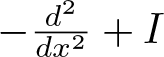 $-{\frac{d^2}{dx^2}}+I$ is invertible with inverse $G_0=(-{\frac{d^2}{dx^2}}+I)^{-1}$ with integral kernel $2^{-1}e^{-\vert x-y\vert}$ on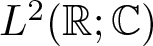 $L^2({\mathbb R} ;{\mathbb C})$, so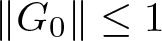 $\Vert G_0\Vert\leq 1$. Hence,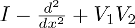 $I-{\frac{d^2}{dx^2}}+V_1V_2$ is invertible with inverse
 \begin{equation*} G_U=\Bigl(I-{\frac{d^2}{dx^2}}+U\Bigr)^{-1}=G_0(I+UG_0)^{-1};\end{equation*}
and 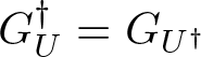 $G_U^\dagger =G_{U^\dagger}$. Then we have
 \begin{equation*}\bigl[G_U^\dagger ,G_U\bigr]=G_U^\dagger G_U\Bigl[ {\frac{d^2}{dx^2}}, U^\dagger -U\Bigr]G_UG_U^\dagger ,\end{equation*}
in which
 \begin{equation*} \Bigl[ {\frac{d^2}{dx^2}}, V_1V_2\Bigr]={\frac{d^2V_1}{dx^2}}V_2+2{\frac{dV_1}{dx}}{\frac{dV_2}{dx}}+V_1{\frac{d^2V_2}{dx^2}} +2{\frac{dV_1}{dx}} V_2{\frac{d}{dx}}+2V_1{\frac{dV_2}{dx}}{\frac{d}{dx}}.\end{equation*}
 By considering their kernels as integral operators, we find that the operators of the form 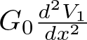 $G_0{\frac{d^2V_1}{dx^2}}$ and $V_2G_0$ are Hilbert–Schmidt, while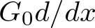 $G_0d/dx$ is bounded. Hence,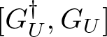 $[G_U^\dagger , G_U]$ is a sum of products of Hilbert–Schmidt operators, hence, is of trace class.
From Lemma 3.5, we deduce that  $G_U=X+iY$ where $X,Y$ are bounded and self-adjoint operators in $L^2$ such that $2i[X,Y]=[G_U^\dagger ,G_U]$ is trace class; one says that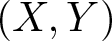 $(X,Y)$ are an almost commuting pair of self-adjoint operators. With nonzero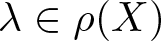 $\lambda\in \rho (X)$ and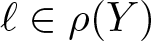 $\ell \in \rho (Y)$, we have $W=\log (I-X/\lambda )$ and $Z=\log (I-Y/\ell )$ such that $[W,Z]\in \mathscr{L}^1(H)$; then $\det (e^We^Ze^{-W}e^{-Z})=\exp(\mathop{\mathrm{trace}} [W,Z])$. Pincus has shown that there exists a compactly supported $g\in L^1({\mathbb R}\times {\mathbb R} ; {\mathbb R} )$ such that
 \begin{align*}
&\det \Bigl( (Y-\ell I)(X-\lambda I)(Y-\ell I)^{-1}(X-\lambda I)^{-1}\Bigr)\\
&\quad=\exp\Bigl({\frac{1}{2\pi i}}\iint_{{\mathbb R}\times{\mathbb R}}g(y,x) {\frac{dydx}{(y-\ell )(x-\lambda )}}\Bigr).\end{align*}
\begin{align*}
&\det \Bigl( (Y-\ell I)(X-\lambda I)(Y-\ell I)^{-1}(X-\lambda I)^{-1}\Bigr)\\
&\quad=\exp\Bigl({\frac{1}{2\pi i}}\iint_{{\mathbb R}\times{\mathbb R}}g(y,x) {\frac{dydx}{(y-\ell )(x-\lambda )}}\Bigr).\end{align*} We introduce the numerical range of  $G_U^\dagger$ as
 \begin{align}
\mathscr{W}(G_U^\dagger )&=\{\langle G_U^\dagger f,f\rangle : f\in H, \Vert f\Vert =1\}\nonumber\\
&=\Biggl\{{\frac{\int_{-\infty}^\infty ( \Vert f(x)\Vert^2+\Vert f'(x)\Vert^2+\langle f(x), U^\dagger (x)f(x)\rangle) dx}
{\int_{-\infty}^\infty \Vert f(x)-f''(x)+U^\dagger (x)f(x)\Vert^2dx}}:\nonumber\\
&\qquad f\in \mathscr{D} (I+\Delta +U^\dagger ); f\neq 0\Biggr\}.
\end{align}
\begin{align}
\mathscr{W}(G_U^\dagger )&=\{\langle G_U^\dagger f,f\rangle : f\in H, \Vert f\Vert =1\}\nonumber\\
&=\Biggl\{{\frac{\int_{-\infty}^\infty ( \Vert f(x)\Vert^2+\Vert f'(x)\Vert^2+\langle f(x), U^\dagger (x)f(x)\rangle) dx}
{\int_{-\infty}^\infty \Vert f(x)-f''(x)+U^\dagger (x)f(x)\Vert^2dx}}:\nonumber\\
&\qquad f\in \mathscr{D} (I+\Delta +U^\dagger ); f\neq 0\Biggr\}.
\end{align} Since 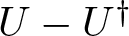 $U-U^\dagger$ is typically non-zero and skew, there is no reason to presume that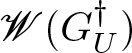 $\mathscr{W}(G_U^\dagger )$ is contained in ${\mathbb R}$.
(i) The spectrum of
$G_U^\dagger$ satisfies
$[0,1]\subseteq \sigma (G_U^\dagger )\subseteq \mathscr{W}(G_U^\dagger )$;(ii) any
$\lambda\in \sigma (G_U^\dagger )\setminus [0,1]$ is an eigenvalue of finite multiplicity.(iii)
$\lambda $ is an eigenvalue of
$G_U^\dagger$ if and only if
\begin{equation*} \iint_{{\mathbb R}\times {\mathbb R}} {\frac{1-g(y,x)}{\vert x+iy-\lambda \vert^2}} dydx \lt \infty .\end{equation*}





Proof. (i) See [Reference Bonsall and Duncan14]. As in the Lemma 3.5, we have  $G_U-G_0\in \mathscr{L}^2(H)$, so $G_U$ is a Hilbert–Schmidt perturbation of the self-adjoint operator $G_0$, hence, their Weyl spectra are equal
 \begin{align}\sigma_{W}(G_U)&=\cap \{\sigma (G_U+K): K\in \mathscr{K} (H)\}\nonumber\\
&=\sigma (G_0)=[0,1].\end{align}
\begin{align}\sigma_{W}(G_U)&=\cap \{\sigma (G_U+K): K\in \mathscr{K} (H)\}\nonumber\\
&=\sigma (G_0)=[0,1].\end{align} One checks that 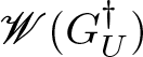 $\mathscr{W}(G_U^\dagger )$ is a compact nonempty set and $\Vert (\lambda I-G_U^\dagger )f\Vert \geq {\hbox{dist}} (\lambda , \mathscr{W}(G_U^\dagger ))$ for all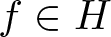 $f\in H$ with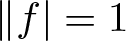 $\Vert f\vert =1$, so the spectrum is contained in the numerical range; see [Reference Bonsall and Duncan14].
(ii) Weyl showed that any  $\lambda\in \sigma (G_U)\setminus \sigma_W(G_U)$ gives an eigenvalue of finite multiplicity.
(iii) This is Carey and Pincus’s criterion for eigenvalues; see [Reference Carey and Pincus19].
Let  $\mathscr{R}_0$ be the subalgebra of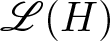 $\mathscr{L} (H)$ that is generated by the set of $r(\Delta^\dagger)$, where $\Delta^\dagger =I-{\frac{d^2}{dx^2}}+U^\dagger$ and $r$ is a complex and proper rational function which is holomorphic on $\sigma (\Delta )$; then let $\mathscr{R}$ be the norm closure of $\mathscr{R}_0$ in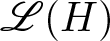 $\mathscr{L} (H)$. Also, if $\lambda $ is a non-zero eigenvalue of $G_U^\dagger$, then $\lambda^{-1}$ is an eigenvalue of $\Delta^\dagger$, so $\lambda^{-1}\in \mathop{\mathrm{spec}} m(\mathscr{R} )$.
Example 3.7. (i) Consider the system
 \begin{equation} {\frac{d}{dx}}\Psi (x;k)=\begin{bmatrix} -ik&q(x)\\-\bar q(x)&ik\end{bmatrix} \Psi (x;k)\end{equation}
which gives the second-order matrix system
 \begin{equation} -{\frac{d^2}{dx^2}}\Psi (x;k) +\begin{bmatrix} -\vert q(x)\vert^2 &q'(x)\\ -\bar q'(x)&-\vert q(x)\vert^2\end{bmatrix}\Psi (x;k)=k^2\Psi (x;k);\end{equation}
 Let  $U$ be the matrix exhibited in (3.10). Then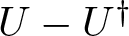 $U-U^\dagger$ is a skew matrix given by the off-diagonal terms. One can select $q'$ to satisfy the hypotheses of Lemma 3.5. See [Reference Zakharov and Shabat70]. (ii) Consider
 \begin{equation*} J{\frac{d\Psi}{dx}}(x;\lambda )=\Omega (x; \lambda )\Psi (x;\lambda )\qquad J=\begin{bmatrix}0&-1\\ 1&0\end{bmatrix} \end{equation*}
where 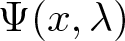 $\Psi (x,\lambda )$ is a real $2\times 2$ matrix such that $\Omega (x; \lambda )=\Omega (x;\lambda )^\top$ and $\mathop{\mathrm{trace}} \Omega (x,\lambda )$ is constant for fixed $\lambda$. Then one can check that
 \begin{equation*} U=J{\frac{d\Omega}{dx}}-J\Omega J\Omega\end{equation*}
is a real symmetric matrix.
Let  $\phi : (0, \infty )\rightarrow M_{n\times n}({\mathbb C} )$. We say that $\phi$ is of Floquet type if there exist $\zeta \in {\mathbb C}$ with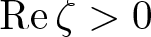 $\mathop{{\rm Re}}\zeta \gt 0$ and $F: {\mathbb R} \rightarrow M_{n\times n}({\mathbb C} ) $ which is once continuously differentiable and $2\pi$-periodic such that $\phi (t)=e^{-\zeta t}F(t)$.
Lemma 3.8. Let  $\phi$ be a Floquet function. Then there exists a linear system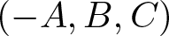 $(-A,B,C)$ such that $\phi$ is impulse response function and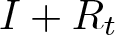 $I+R_t$ gives a convergent determinant.
Proof. An infinite determinant converges provided that the product of the diagonal entries converges absolutely and the sum of the off-diagonal entries converges absolutely; see [Reference Whittaker and Watson69, 2.81]. For notational simplicity, we suppose that  $F$ is scalar-valued with Fourier expansion $F(x)=\sum_{n=-\infty}^\infty a_ne^{inx}$. We choose $3/2 \lt r \lt 2$ and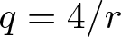 $q=4/r$ and $\beta =(3-r)/2$ such that
 \begin{equation*}\sum_n \vert a_n\vert^{r/2}\leq \Bigl(\sum_n \vert a_n\vert^2(1+\vert n\vert)^{\beta q}\Bigr)^{1/q}\Bigl(\sum_n(1+\vert n\vert )^{-\beta q/(q-1)}\Bigr)^{(q-1)/q)}\end{equation*}
converges. Let  $H=\ell^2({\mathbb Z} ;{\mathbb C} )$ and consider $\mathscr{D} (A)=\{(\xi_m)_{m=-\infty} ^\infty \in H : (m\xi_m)\in H\}$
 \begin{align}
A: \mathscr{D} (A)\rightarrow H:& \quad (\xi_m)\mapsto ((\zeta -im)\xi_m)\nonumber\\
B: {\mathbb C} \mapsto H:&\quad b\mapsto (\vert a_m\vert^{1/2} b)_{m=-\infty}^\infty\nonumber\\
C: H\rightarrow {\mathbb C} : &\quad (\xi_m)\mapsto \sum_m {\frac{a_m\xi_m}{\sqrt{\vert a_m\vert}}}.
\end{align}
\begin{align}
A: \mathscr{D} (A)\rightarrow H:& \quad (\xi_m)\mapsto ((\zeta -im)\xi_m)\nonumber\\
B: {\mathbb C} \mapsto H:&\quad b\mapsto (\vert a_m\vert^{1/2} b)_{m=-\infty}^\infty\nonumber\\
C: H\rightarrow {\mathbb C} : &\quad (\xi_m)\mapsto \sum_m {\frac{a_m\xi_m}{\sqrt{\vert a_m\vert}}}.
\end{align} Then we have  $\phi (t)=Ce^{-tA}B=\sum_m a_m e^{-t(\zeta -im)}=e^{-\zeta t}F(t)$, and we can represent $R_t$ as the following matrix with respect to the standard basis of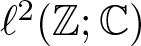 $\ell^2({\mathbb Z}; {\mathbb C} )$:
 \begin{align}
R_t&=\int_t^\infty e^{-uA}BCe^{-uA}\, du\nonumber\\
&=\Biggl[\int_t^\infty e^{-(2\lambda -im-in)u} {\frac{a_m\sqrt{\vert a_n\vert}}{\sqrt{\vert a_m\vert}}}du \Biggr]_{n,m=-\infty}^\infty\nonumber\\
&=\Biggl[ {\frac{e^{-(2\lambda -im-in)t}}{2\zeta -im-in} } {\frac{a_m\sqrt{\vert a_n\vert}}{\sqrt{\vert a_m\vert }}}\Biggr]_{m,n=-\infty}^\infty
\end{align}
\begin{align}
R_t&=\int_t^\infty e^{-uA}BCe^{-uA}\, du\nonumber\\
&=\Biggl[\int_t^\infty e^{-(2\lambda -im-in)u} {\frac{a_m\sqrt{\vert a_n\vert}}{\sqrt{\vert a_m\vert}}}du \Biggr]_{n,m=-\infty}^\infty\nonumber\\
&=\Biggl[ {\frac{e^{-(2\lambda -im-in)t}}{2\zeta -im-in} } {\frac{a_m\sqrt{\vert a_n\vert}}{\sqrt{\vert a_m\vert }}}\Biggr]_{m,n=-\infty}^\infty
\end{align}By Young’s convolution inequality, we have
 \begin{equation} \sum_{m,n} {\frac{\sqrt{\vert a_n\vert}\sqrt{\vert a_m\vert}} {\vert 2\zeta -im-in\vert}}\leq \bigl\Vert (\sqrt{\vert a_n\vert})\bigr\Vert^2_{\ell^r}\Bigl\Vert \Bigl({\frac{1}{\vert 2\zeta -im\vert}}\Bigr) \Bigr\Vert_{\ell^p} \end{equation}
where  $1/p=2-2/r \lt 1$. Hence, the matrix that represents $R_t$ has absolutely summable entries, as stated.
Example 3.9. Let  $U_1\in M_{n\times n}({\mathbb C} )$ and let $U_0:{\mathbb R} \rightarrow M_{n\times n}({\mathbb C} )$ be continuous and $2\pi$ periodic. Then the differential equation
 \begin{equation} {\frac{d^2\Phi }{dt^2}}=(\lambda U_1+U_0(t))\Phi (t)\end{equation}
gives rise to a first-order periodic system
 \begin{equation} {\frac{d\Psi}{dt}}=\begin{bmatrix} 0&I_n\\ \lambda U_1+U_0(t)&0\end{bmatrix}\Psi\end{equation}
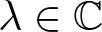
where  $\Psi (t;\lambda )\in M_{2n\times 2n}({\mathbb C} )$ is holomorphic in $\lambda$. Then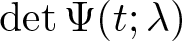 $\det \Psi (t; \lambda )$ is constant in $t$, and for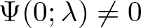 $\Psi (0;\lambda )\neq 0$, we have a $2n$-sheeted cover of ${\mathbb C}$ given by
 \begin{equation*} \bigl\{(\lambda , \rho ): \det \bigl( \rho \Psi (0; \lambda )-\Psi (2\pi ; \lambda )\bigr) =0\bigr\}.\end{equation*}
 Suppose that  $\lambda$ is not a branch point, so that there are truly $(2n)$ distinct choices of $\rho$. Then we write the modular matrix as $M(\lambda )= \Psi (0; \lambda)^{-1}\Psi (2\pi ;\lambda )$.
(i) Suppose that
$M(\lambda )$ has distinct eigenvalues, not all of them unimodular, for some
$\lambda\in {\mathbb C}$. Then there exists
$(-A,B,C)$ such that
$I+R_t$ has a convergent determinant and impulse response function
$\phi$.(ii) Suppose that
$U_0(x)=\sum_{k=-\ell}^\ell A_ke^{ikx}$ is a trigonometric polynomial such that
$A_\ell$ and
$A_{-\ell}$ are invertible, and
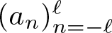
$(a_n)_{n=-\ell}^\ell$ are given. Then the full sequence
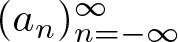
$(a_n)_{n=-\infty}^\infty$ is determined by a recurrence relation.





Proof. (i) We introduce an invertible  $V\in M_{2n\times 2n}({\mathbb C} )$ and $D=\mathop{\mathrm{diag}} (\rho_1, \dots , \rho_{2n})$ such that $M=VDV^{-1}$. The product of the eigenvalues is $\prod_{j=1}^{2n}\rho_j=\det M(\lambda )=1$, so either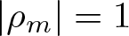 $\vert\rho_m\vert=1$ for all $m$, or there exists $j$ such that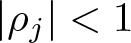 $\vert\rho_j\vert \lt 1$, as in the hypothesis. With $\zeta_j=-(2\pi )^{-1}\log\rho_j$ and $D(x)=\mathop{\mathrm{diag}} ( e^{-\zeta_jx})$, we have a $2\pi$-periodic $G(x)=\Psi (x)VD(-x)$. In particular, let $E_j$ be the diagonal matrix that has $1$ in place $j$ and zeros elsewhere; then let $C_j=VE_jV^{-1}$ so that $\Psi_j(x)=\Psi (x)C_j$ gives a solution of the ODE with $\Psi_j(x)=e^{-\zeta_jx}G(x)E_jV^{-1}$. Then we write the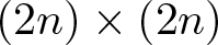 $(2n)\times (2n)$ matrix in terms of four $n\times n$ blocks
 \begin{equation*} \Phi_j(x)=\begin{bmatrix} \Phi_j(x) & \Xi_j(x) \\ \Phi'_j(x)& \Xi'_j(x)\end{bmatrix}\end{equation*}
where  $\Phi_j(x)= e^{-\zeta_jx}F_j(x)$ has $F_j:{\mathbb R}\rightarrow M_{n\times n}({\mathbb C} )$ is continuous and $2\pi$-periodic and ${\frac{d^2\Phi_j}{dt^2}}=(\lambda U_1+U_0(t))\Phi_j(t)$. For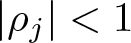 $\vert\rho_j\vert \lt 1$, we obtain a Floquet solution.
(ii) We consider the recurrence relation
 \begin{equation} \zeta_j^2a_n-2in\zeta_ja_n-n^2a_n-\lambda a_n-\sum_{k=-\ell}^\ell A_ka_{n-k}=0,\end{equation}
which we can solve for  $a_{n+\ell}$ since $A_{-\ell}$ is invertible, giving , with
 \begin{equation} B_\ell (n)=-A_{-\ell}^{-1}\bigl(\zeta_j^2 -2i\zeta_jn-n^2-\lambda-A_0\bigr)\end{equation}
the related matrix version
 \begin{equation} \begin{bmatrix} a_{n+\ell }\\ \vdots \\ a_{n+1}\\ \vdots \\ a_{n-\ell +1}\end{bmatrix}= \begin{bmatrix} -A_{-\ell}^{-1}A_{-\ell +1}& \dots & B_\ell (n) &\dots & -A_{-\ell}^{-1}A_\ell\\
1&0&\dots &\dots &0\\ 0&1&0&\dots &\vdots\\ \vdots &{}&\ddots&\ddots &\vdots\\ 0&\dots & 0&1&0\end{bmatrix}
\begin{bmatrix} a_{n+\ell-1} \\ \vdots \\ a_{n}\\ \vdots \\ a_{n-\ell }\end{bmatrix}.\end{equation}
\begin{equation} \begin{bmatrix} a_{n+\ell }\\ \vdots \\ a_{n+1}\\ \vdots \\ a_{n-\ell +1}\end{bmatrix}= \begin{bmatrix} -A_{-\ell}^{-1}A_{-\ell +1}& \dots & B_\ell (n) &\dots & -A_{-\ell}^{-1}A_\ell\\
1&0&\dots &\dots &0\\ 0&1&0&\dots &\vdots\\ \vdots &{}&\ddots&\ddots &\vdots\\ 0&\dots & 0&1&0\end{bmatrix}
\begin{bmatrix} a_{n+\ell-1} \\ \vdots \\ a_{n}\\ \vdots \\ a_{n-\ell }\end{bmatrix}.\end{equation} This tells us how to progress one step forwards along the sequence 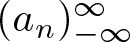 $(a_n)_{-\infty}^\infty$; while a corresponding matrix relation involving $A_\ell^{-1}$ tells us how to take one step backwards. Then the complete sequence $(a_n)$ gives the entries of $R_t$ in (3.12).
Remark 3.11. If  $U_0(x)$ is a trigonometric polynomial with matrix coefficients, then (3.14) becomes a variant of Mathieu’s equation. This occurs for an instance of the differential equation (3.14) that is used in the theory of graphene to analyse spinors and determine the band structure of their energy levels [Reference López–Rodriguez and Naumis43, (12)]]. See [Reference Roy62, page 135] for instances in orbital motion where the hypotheses of Proposition 3.10 are not satisfied.
4. Zakharov–Shabat system
The Zakharov–Shabat system was introduced in [Reference Zakharov and Shabat70], and expressed in terms of operators in [Reference Bauhardt and Pöppe1]. The following definition is suggested by [Reference Jacob, Partington and Pott39].
Definition 4.1. Let 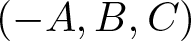 $(-A,B,C)$ be a linear system with input and output space $H_0$ and state space $H$. A bounded linear operator $C:\mathscr{D} (A)\rightarrow H_0$ is admissible for $e^{-tA}$ if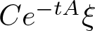 $Ce^{-tA}\xi$ belongs to $L^2((0, \infty ); H_0)$ for all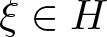 $\xi\in H$ and there exists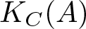 $K_C(A)$ such that
 \begin{equation} \int_0^\infty \Vert Ce^{-tA} \xi \Vert^2_{H_0}dt\leq K_C(A)^2\Vert \xi\Vert^2_{H}\qquad (\xi\in H).\end{equation}
Lemma 4.2. Suppose for the remainder of this section that  $C$ is admissible for $e^{-tA}$ and $B^\dagger$ is admissible for $e^{-tA^\dagger}$. Then
(i) the operators
$R_x:H\rightarrow H$
are bounded,
\begin{equation*} R_x\xi =\int_x^\infty e^{-tA}BCe^{-tA}\xi dt\qquad (x \gt 0; \xi\in H)\end{equation*}(ii) with
$\phi (x)=Ce^{-xA}B$, the Hankel operator
$\Gamma_\phi :L^2((0, \infty ); H_0)\rightarrow L^2((0, \infty ); H_0)$, defined by
is also bounded.
\begin{equation*} \Gamma_\phi f(x)=\int_0^\infty \phi (x+y)f(y)\, dy\end{equation*}(iii) Suppose that
(4.2)converges. Then\begin{equation}\int_0^\infty (\Vert Ce^{-tA}\Vert^2_{\mathscr{L}^2(H,H_0)}+\Vert B^\dagger e^{-tA^\dagger}\Vert^2_{\mathscr{L}^2(H,H_0)})dt\end{equation}
$R_x$ and
$\Gamma_\phi$ are trace class.






Proof. The hypothesis is equivalent to the statement that the observability Gramian  $Q_x$ and the observability Gramian $M_x$ are bounded linear operators on $H$, as defined by the weakly convergent integrals
 \begin{equation} Q_x=\int_x^\infty e^{-tA^\dagger}C^\dagger Ce^{-tA}\,dt, \qquad M_x=\int_x^\infty e^{-tA}BB^\dagger e^{-tA^\dagger} dt.\end{equation}
 Then the observability operators  $\Theta_x:L^2((0, \infty ):H_0)\rightarrow H$ and the controllability operators $\Xi_x: L^2((0, \infty ); H_0)\rightarrow H$ given by
 \begin{equation*} \Theta_xf=\int_x^\infty e^{-tA^\dagger} C^\dagger f(t)\, dt, \quad \Xi_xf=\int_x^\infty e^{-tA}Bf(t)\, dt\end{equation*}
are bounded, since 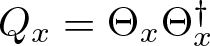 $Q_x=\Theta_x\Theta_x^\dagger$ and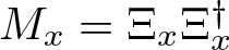 $M_x=\Xi_x\Xi_x^\dagger$. Here, $Q_x$ and $M_x$ are self-adjoint and non-negative.
(i) Hence, the operator 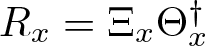 $R_x=\Xi_x\Theta_x^\dagger$ is bounded on $H$.
$H$.
(ii) Also  $\Theta_x^\dagger\Xi_x$ is bounded on $L^2((0, \infty );H_0)$, so the Hankel operator $\Gamma_\phi$ is bounded.
(iii) Here,  $Q_x$ and $M_x$ are trace class, so $\Theta_x$ and $\Xi_x$ are Hilbert–Schmidt; hence, $R_x$ and $\Gamma_\phi$ are trace class, with
 \begin{equation*} \Vert R_x\Vert_{\mathscr{L}^1}\leq \Vert \Xi_x\Vert_{\mathscr{L}^2}\Vert \Theta_x^\dagger \Vert_{\mathscr{L}^2}, \quad \Vert\Gamma_{\phi}\Vert_{\mathscr{L}^1}\leq \Vert \Xi_0\Vert_{\mathscr{L}^2}\Vert\Theta_0\Vert_{\mathscr{L}^2}.\end{equation*}
 The hypothesis for Lemma 4.2(iii) is somewhat coarse. In Proposition 4.5(iv) and Proposition 6.1, we only need  $Q_x$ and $M_x$ to be Hilbert–Schmidt, and in Section 9, we give examples where this occurs under milder hypotheses. In the abstract, we express our results in terms of Hankels, instead of the less familiar $R_x$.
Now let 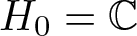 $H_0={\mathbb C}$. From the linear system
 \begin{equation*}\bigl(-\hat A, \hat B, \hat C\bigr)= \Biggl( \begin{bmatrix} -A^\dagger& 0\\ 0&-A\end{bmatrix}, \begin{bmatrix} C^\dagger &0\\ 0&B\end{bmatrix} , \begin{bmatrix} 0&C\\ \lambda B^\dagger &0\end{bmatrix}\Biggr)\end{equation*}
with input and output space  $\mathbb{C}^2$ and state space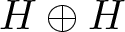 $H\oplus H$, we introduce $\phi (x)=Ce^{-xA}B$ and
 \begin{equation*}\Phi (x)=\begin{bmatrix} 0&\phi (x)\\ \lambda\overline{\phi (x)}&0\end{bmatrix},\qquad \hat R_x=\begin{bmatrix} 0&M_x\\ \lambda Q_x&0\end{bmatrix}\end{equation*}
so
 \begin{equation*} \hat F_x=(I+\hat R_x)^{-1}=\begin{bmatrix} (I-\lambda Q_xM_x)^{-1}& -(I-\lambda Q_xM_x)^{-1}Q_x\\ -\lambda (I-\lambda M_xQ_x)^{-1}M_x& (I-\lambda M_xQ_x)^{-1}\end{bmatrix}.\end{equation*}
 We note that  $M_x, Q_x\geq 0$ as operators, so $\sigma (M_xQ_x)\setminus \{0\}=\sigma (M_x^{1/2}Q_xM_x^{1/2})\setminus \{0\}\subset (0, \infty )$, hence, $I-\lambda M_xQ_x$ is invertible for all $\lambda\in {\mathbb C} \setminus (0, \infty )$
Definition 4.3. Let  $\mathscr{A}$ be the complex algebra formed by linear combinations of products of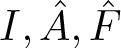 $I,\hat A,\hat F$, and let ${\frac{d}{dx}}$ be a derivation on $\mathscr{A}$ such that
 \begin{equation}{\frac{d\hat A}{dx}}=0,\end{equation}
 \begin{equation}{\frac{d\hat F}{dx}}=\hat A\hat F+\hat F\hat A-2\hat F\hat A\hat F.\end{equation}
 We also introduce the associative product  $\ast$ on ${\mathscr{A}}$ by
 \begin{equation} Y\ast Z=Y(\hat A\hat F+\hat F\hat A-2\hat F\hat A\hat F)Z\end{equation}
and the differential expressions
 \begin{equation}D_xY=(\hat A-2\hat A\hat F)Y+{\frac{dY}{dx}} +Y(\hat A-2\hat F\hat A).\end{equation}
Then we let
 \begin{equation} \lfloor Y\rfloor = \hat Ce^{-x\hat A}\hat F_xY\hat F_xe^{-x\hat A}\hat B\qquad (x \gt 0).\end{equation}
This bracket operation is related to that of Pöppe [Reference Pöppe59, p 622] and Definition 2.3 (ii), and our identities that correspond to his Theorem 3.1 are summarized in the following Proposition.
Proposition 4.4. There is a homomorphism of differential rings
 \begin{equation*} \lfloor \cdot \rfloor :\bigl(\mathscr{A}, \ast , D_x \bigr)\rightarrow \bigl( C^\infty ((0, \infty ); M_{2\times 2}(\mathbb{C})), \cdot ,d/dx\bigr) \end{equation*}
such that
 \begin{equation} {\frac{d}{dx}}\lfloor Y\rfloor =\lfloor D_xY\rfloor, \qquad \lfloor Y\ast Z\rfloor =\lfloor Y\rfloor \lfloor Z\rfloor .\end{equation}
Proof. Using the Lyapunov identity
 \begin{equation} {\frac{d\hat R_x}{dx}}=-\hat A \hat R_x-\hat R_x\hat A,\end{equation}
one verifies (4.5). We can also write
 \begin{equation*} {\frac{d\hat R_x}{dx}} =-e^{-x\hat A}\hat B\hat Ce^{-x\hat A};\end{equation*}
given this, it is straightforward to verify (4.9) by a direct calculation as in [Reference Blower and Newsham13, Lemma 4.1].
Now we let  $T(x,y)=-\hat Ce^{-x\hat A}(I+\hat R_x)^{-1}e^{-y\hat A}\hat B$, or more explicitly
 \begin{align*} & T(x,y) = \nonumber\\
& \begin{bmatrix} \lambda Ce^{-xA}(I-\lambda M_xQ_x)^{-1} M_xe^{-yA^\dagger} C^\dagger & - Ce^{-xA}(I-\lambda M_xQ_x)^{-1}e^{-yA}B\\
-\lambda B^\dagger e^{-xA^\dagger} (I-\lambda Q_xM_x)^{-1}e^{-yA^\dagger}C^\dagger & \lambda B^\dagger e^{-xA^\dagger} (I-\lambda Q_xM_x)^{-1}Q_xe^{-yA}B
\end{bmatrix} .
\end{align*}
\begin{align*} & T(x,y) = \nonumber\\
& \begin{bmatrix} \lambda Ce^{-xA}(I-\lambda M_xQ_x)^{-1} M_xe^{-yA^\dagger} C^\dagger & - Ce^{-xA}(I-\lambda M_xQ_x)^{-1}e^{-yA}B\\
-\lambda B^\dagger e^{-xA^\dagger} (I-\lambda Q_xM_x)^{-1}e^{-yA^\dagger}C^\dagger & \lambda B^\dagger e^{-xA^\dagger} (I-\lambda Q_xM_x)^{-1}Q_xe^{-yA}B
\end{bmatrix} .
\end{align*} There exists  $x_0$ such that $\Vert Q_xM_x\Vert_{\mathscr{L}(H)} \lt 1$ for all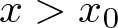 $x \gt x_0$ since $Q_x, M_x\rightarrow 0$ as $x\rightarrow\infty $, so $T$ is well defined.
(i) Then the Gelfand–Levitan equation is satisfied
\begin{equation*} 0=\Phi (x+y)+T(x,y)+\int_x^\infty T(x,z) \Phi (z+y)\, dz\qquad (x_0 \lt x \lt y).\end{equation*}(ii) The nonlinear differential equation is satisfied
(4.11)\begin{equation} {\frac{\partial^2T}{\partial x^2}} -{\frac{\partial^2T}{\partial y^2}}=\Bigl(-2{\frac{d}{dx}}T(x,x)\Bigr) \, T(x,y).\end{equation}(iii) Suppose that
$\hat C\hat A $ and
$\hat A\hat B$ are bounded linear operators, and let
$\Delta$ be the differential operator
\begin{equation*} \Delta \Psi (x)=-{\frac{\partial^2\Psi }{\partial x^2}}+\Bigl(-2{\frac{d}{dx}}T(x,x)\Bigr) \Psi (x).\end{equation*}Then
$(\cos (t\sqrt \Delta ))_{t\geq 0}$ is a cosine family on
$L^2((x_0, \infty ); {\mathbb C}^2)$ such that
\begin{equation*}\Vert \cos (t\sqrt{\Delta })\Vert_{\mathscr{L} (L^2)}\leq Me^{\omega t}\qquad (t\geq 0).\end{equation*}(iv) Suppose that
$Q_x$ and
$M_x$ are Hilbert–Schmidt operators on
$H$. Then the Fredholm determinant satisfies
(4.12)\begin{equation} \mathop{\mathrm{trace}} T(x,x)={\frac{d}{dx}}\log\det (I-\lambda Q_xM_x).
\end{equation}






Proof. (i) This is a direct computation by substituting the functions in terms of 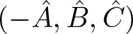 $(-\hat A,\hat B, \hat C)$.
(ii) This follows from (i) by the uniqueness of solutions.
(iii) Let  $U(x)=-2{\frac{d}{dx}}T(x,x)$. We have
 \begin{align}{\frac{d}{dx}}T(x,x)&=\hat C\hat Ae^{-x\hat A}(I+\hat R_x)^{-1}e^{-x\hat A}\hat B+\hat Ce^{-x\hat A}(I+\hat R_x)^{-1}e^{-x\hat A}\hat B\nonumber\\
&\qquad -\hat Ce^{-x\hat A}(I+\hat R_x)^{-1}e^{-x\hat A}\hat B\hat Ce^{-x\hat A}(I+\hat R_x)^{-1}e^{-x\hat A}\hat B,\end{align}
\begin{align}{\frac{d}{dx}}T(x,x)&=\hat C\hat Ae^{-x\hat A}(I+\hat R_x)^{-1}e^{-x\hat A}\hat B+\hat Ce^{-x\hat A}(I+\hat R_x)^{-1}e^{-x\hat A}\hat B\nonumber\\
&\qquad -\hat Ce^{-x\hat A}(I+\hat R_x)^{-1}e^{-x\hat A}\hat B\hat Ce^{-x\hat A}(I+\hat R_x)^{-1}e^{-x\hat A}\hat B,\end{align}where each term is uniformly bounded for 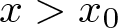 $x \gt x_0$; hence, $U(x)\in L^\infty ({\mathbb R} ;M_{2\times 2}({\mathbb C} ))$.
For all  $\Psi_0\in L^2({\mathbb R}; M_{2\times 2} ({\mathbb C} ))$, there exists a unique solution to
 \begin{align}
{\frac{\partial^2}{\partial t^2}}\Psi (t,x)-{\frac{\partial^2}{\partial x^2}}\Psi (t,x) +U(x)\Psi (x,t)&=0\nonumber\\
\Psi (0,x)&=\Psi_0(x)\nonumber\\
{\frac{\partial}{\partial t}}\Psi (0,x)&=0.
\end{align}
\begin{align}
{\frac{\partial^2}{\partial t^2}}\Psi (t,x)-{\frac{\partial^2}{\partial x^2}}\Psi (t,x) +U(x)\Psi (x,t)&=0\nonumber\\
\Psi (0,x)&=\Psi_0(x)\nonumber\\
{\frac{\partial}{\partial t}}\Psi (0,x)&=0.
\end{align} When  $U=0$, the unique solution is given by D’Alembert’s solution
 \begin{equation*}\Psi (t,x)=(1/2)(\Psi_0(x-t)+\Psi_0(x+t)).\end{equation*}
 By a standard result of operator semigroup theory [Reference Goldstein35, theorem 8.5], one can perturb 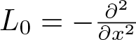 $L_0=-{\frac{\partial^2}{\partial x^2}}$ by adding the bounded operator of multiplication by $U$, and obtain a generator $L_1$ of a cosine family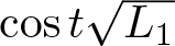 $\cos t\sqrt{L_1}$ such that $\Vert \cos (t\sqrt{L_1})\Vert\leq Me^{\omega t}$ for some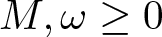 $M,\omega\geq 0$ and all $t\in {\mathbb R}$.
(iv) By hypothesis,  $Q_xM_x\in \mathscr{L}^1(H)$, so the determinant is well defined. To prove this identity, we rearrange operators in the following expression
 \begin{align}{\hbox{trace}}\, & T(x,x)\nonumber\\
&=\lambda Ce^{-xA}(I-\lambda M_xQ_x)^{-1}+\lambda B^\dagger e^{-xA^\dagger} (I-\lambda Q_xM_x)^{-1}Q_xe^{-xA}B\nonumber\\
&=\lambda{\hbox{trace}}\bigl( (I-Q_xM_x)^{-1}M_xe^{-xA^\dagger}C^\dagger Ce^{-xA}+\nonumber\\
&\quad (I-\lambda Q_xM_x)^{-1}Q_xe^{-xA}BB^\dagger e^{-xA^\dagger}\bigr)\nonumber\\
&=-\lambda {\hbox{trace}}\Bigl( (I-\lambda M_xQ_x)^{-1}M_x{\frac{dQ_x}{dx}}+(I-\lambda Q_xM_x)^{-1}Q_x{\frac{dM_x}{dx}}\Bigr)\nonumber\\
&= -\lambda {\hbox{trace}}\Bigl( M_x(I-\lambda Q_xM_x)^{-1}{\frac{dQ_x}{dx}}+(I-\lambda Q_xM_x)^{-1}Q_x{\frac{dM_x}{dx}}\Bigr)\nonumber\\
&=-\lambda {\hbox{trace}}\Bigl((I-\lambda Q_xM_x)^{-1}\Bigl({\frac{dQ_x}{dx}}M_x+Q_x{\frac{dM_x}{dx}}\Bigr)\Bigr)\nonumber\\
&={\frac{d}{dx}}\log\det (I-\lambda Q_xM_x).\end{align}
\begin{align}{\hbox{trace}}\, & T(x,x)\nonumber\\
&=\lambda Ce^{-xA}(I-\lambda M_xQ_x)^{-1}+\lambda B^\dagger e^{-xA^\dagger} (I-\lambda Q_xM_x)^{-1}Q_xe^{-xA}B\nonumber\\
&=\lambda{\hbox{trace}}\bigl( (I-Q_xM_x)^{-1}M_xe^{-xA^\dagger}C^\dagger Ce^{-xA}+\nonumber\\
&\quad (I-\lambda Q_xM_x)^{-1}Q_xe^{-xA}BB^\dagger e^{-xA^\dagger}\bigr)\nonumber\\
&=-\lambda {\hbox{trace}}\Bigl( (I-\lambda M_xQ_x)^{-1}M_x{\frac{dQ_x}{dx}}+(I-\lambda Q_xM_x)^{-1}Q_x{\frac{dM_x}{dx}}\Bigr)\nonumber\\
&= -\lambda {\hbox{trace}}\Bigl( M_x(I-\lambda Q_xM_x)^{-1}{\frac{dQ_x}{dx}}+(I-\lambda Q_xM_x)^{-1}Q_x{\frac{dM_x}{dx}}\Bigr)\nonumber\\
&=-\lambda {\hbox{trace}}\Bigl((I-\lambda Q_xM_x)^{-1}\Bigl({\frac{dQ_x}{dx}}M_x+Q_x{\frac{dM_x}{dx}}\Bigr)\Bigr)\nonumber\\
&={\frac{d}{dx}}\log\det (I-\lambda Q_xM_x).\end{align}Note that we can write
 \begin{equation*} T(x,y)=\begin{bmatrix}Y(x,y)&V(x,y)\\ \lambda X(x,y)&W(x,y)\end{bmatrix}\end{equation*}
where  $X(x,x)=\overline{V(x,x)}$. Within $M_{2\times 2} (\mathbb{C})$ we note two real-linear subspaces that have real dimension four, namely the quaternions ${\mathbb H}$ and the $2\times 2$ complex Hermitian matrices. These arise as follows.
Proposition 4.6. Suppose that  $CA^j$ is admissible for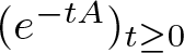 $(e^{-tA})_{t\geq 0}$ and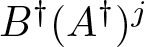 $B^\dagger (A^\dagger )^j$ is admissible for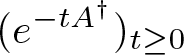 $(e^{-tA^\dagger })_{t\geq 0}$ for $j=0, 1, \dots.$
(i) Then the matrix function
$\Psi$, defined by an integral that converges in the
$L^2$ sense,
satisfies Schrödinger’s equation with a matrix potential
\begin{equation*} \Psi (x)=\begin{bmatrix} e^{ikx}&0\\ 0&e^{-ikx}\end{bmatrix}+\int_x^\infty T(x,y)\begin{bmatrix} e^{iky}&0\\ 0&e^{-iky}\end{bmatrix}dy,\end{equation*}
$U(x)=-2{\frac{d}{dx}}T(x,x)$,
\begin{equation*} -{\frac{d^2}{dx^2}} \Psi (x)+ \Bigl( -2{\frac{d}{dx}}T(x,x)\Bigr)\Psi (x)=k^2\Psi (x).\end{equation*}(ii) Let
$\lambda =1$; then
$U(x)$ is a Hermitian matrix.(iii) Let
$\lambda =-1$; then
$U(x)$ is a quaternion, and the differential ring generated by
$U$ consists of quaternions.





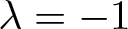


Proof. (i) First, we check convergence of the integral defining  $\Psi$. By hypothesis, there exists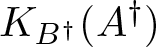 $K_{B^\dagger}(A^\dagger )$ such that
 \begin{equation*} \int_0^\infty \Vert B^\dagger e^{-tA^\dagger}\xi \Vert^2_{H_0}dt\leq K_{B^\dagger}(A^\dagger )^2\Vert \xi \Vert^2_H \qquad (\xi\in H).\end{equation*}
 Let  $RHP=\{z\in {\mathbb C} :\mathop{{\rm Im}} z \gt 0\}$ and $H^2(RHP: H_0 )$ be the Hardy space of holomorphic $f:RHP\rightarrow H_0$ such that $\sup_{x \gt 0} \int_{-\infty}^\infty \Vert f(x+iy)\Vert^2_{H_0}\, dy \lt \infty $. Then by the Paley-Wiener theorem,
 \begin{equation*}\int_x^\infty e^{-st} B^\dagger e^{-tA^\dagger }\xi dt=e^{-sx}B^\dagger (sI+A^\dagger )^{-1} e^{-xA^\dagger}\xi\qquad (\mathop{{\rm Re}} s \gt 0)\end{equation*}
gives a function in the Hardy space  $H^2(RHP; H_0)$. Choosing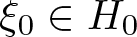 $\xi_0\in H_0$ and $\xi =(I+R_x^\dagger )^{-1}e^{-xA^\dagger} C^\dagger \xi_0$, we have
 \begin{equation*} e^{-sx}B^\dagger (sI+A^\dagger)^{-1}e^{-xA^\dagger} (I+R_x^\dagger )^{-1} e^{-xA^\dagger} C^\dagger \xi_0\in H^2(RHP; H_0).\end{equation*}
for  $s=\varepsilon +ik$ and the boundary values with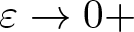 $\varepsilon\rightarrow 0+$ give
 \begin{equation*} \Bigl( \int_x^\infty T(x,y)e^{iky}\, dy\Bigr)^\dagger \xi_0.\end{equation*}
Then the differential equation follows from (4.11).
Suppose that 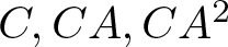 $C,CA, CA^2$ are admissible for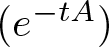 $(e^{-tA})$ and $B^\dagger, B^\dagger A^\dagger B^\dagger (A^\dagger )^2$ are admissible for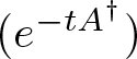 $(e^{-tA^\dagger})$. Then $U$ is twice differentiable, with the following derivatives
 \begin{align}
U&=-4\bigl\lfloor A\bigr\rfloor ,\nonumber\\
{\frac{dU}{dx}}&=-8\bigl\lfloor A(I-2F)A\big\rfloor ,
\end{align}
\begin{align}
U&=-4\bigl\lfloor A\bigr\rfloor ,\nonumber\\
{\frac{dU}{dx}}&=-8\bigl\lfloor A(I-2F)A\big\rfloor ,
\end{align} \begin{equation}
{\frac{d^2U}{dx^2}}=-16\bigl\lfloor A(I-2F)A(I-2F)A\bigr\rfloor +16\bigl\lfloor A(AF+FA-2FAF)A\bigr\rfloor
\end{equation}
\begin{equation}
{\frac{d^2U}{dx^2}}=-16\bigl\lfloor A(I-2F)A(I-2F)A\bigr\rfloor +16\bigl\lfloor A(AF+FA-2FAF)A\bigr\rfloor
\end{equation}which includes terms such as
 \begin{equation*} 16\bigl\lfloor A^2FA\bigr\rfloor =16Ce^{-xA}\Bigl( \bigl([F,A^2]+A^2F\bigr) F\bigl( [A,F]+FA\bigr)\Bigr)e^{-xA}B\end{equation*}
where  $[F,A^2]=-F[R,A^2]F$, and $A^2R$ and $RA^2$ are bounded operators. By induction, one can prove that $D_x^nA=2^{n}A^{n+1}+p_n(A,F)$ where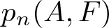 $p_n(A,F)$ is a polynomial in the noncommuting variables $A$ and $F$ such that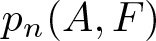 $p_n(A,F)$ has degree less than or equal to $n+1$ in the variable $A$ and monomials in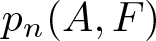 $p_n(A,F)$ have factors $I,A, \dots , A^n$ but not $A^{n+1}$.
(ii) For  $\lambda =1$, we have $T(x,x)=T(x,x)^\dagger$, and $-2{\frac{d}{dx}}T(x,x)=-2{\frac{d}{dx}}T(x,x)^\dagger$. Furthermore, we can extract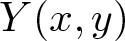 $Y(x,y)$ and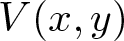 $V(x,y)$ from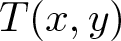 $T(x,y)$ and solve the Gelfand–Levitan equation
 \begin{align}0=&\begin{bmatrix} Y(x,y)&V(x,y)\\ \overline{V}(x,y)&\overline{Y}(x,y)\end{bmatrix} +\begin{bmatrix} 0&\phi (x+y)\\ \overline{\phi} (x+y) &0\end{bmatrix}\nonumber\\
&\quad +\int_x^\infty
\begin{bmatrix} Y(x,z)&V(x,z)\\ \overline{V}(x,z)&\overline{Y}(x,z)\end{bmatrix}\begin{bmatrix} 0&\phi (z+y)\\ \overline{\phi} (z+y) &0\end{bmatrix}\, dz.\end{align}
\begin{align}0=&\begin{bmatrix} Y(x,y)&V(x,y)\\ \overline{V}(x,y)&\overline{Y}(x,y)\end{bmatrix} +\begin{bmatrix} 0&\phi (x+y)\\ \overline{\phi} (x+y) &0\end{bmatrix}\nonumber\\
&\quad +\int_x^\infty
\begin{bmatrix} Y(x,z)&V(x,z)\\ \overline{V}(x,z)&\overline{Y}(x,z)\end{bmatrix}\begin{bmatrix} 0&\phi (z+y)\\ \overline{\phi} (z+y) &0\end{bmatrix}\, dz.\end{align} Here, 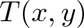 $T(x,y)$ and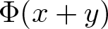 $\Phi (x+y)$ can be expressed as real linear combinations of the matrices
 \begin{equation*}\sigma_0=\begin{bmatrix} 1&0\\ 0&1\end{bmatrix},\quad
\sigma_1=\begin{bmatrix} 0&1\\ 1&0\end{bmatrix}, \quad
\sigma_2=\begin{bmatrix} 0&-i\\ i&0\end{bmatrix}\quad
i\sigma_3 =\begin{bmatrix} i&0\\ 0&-i\end{bmatrix},\quad
\end{equation*}
\begin{equation*}\sigma_0=\begin{bmatrix} 1&0\\ 0&1\end{bmatrix},\quad
\sigma_1=\begin{bmatrix} 0&1\\ 1&0\end{bmatrix}, \quad
\sigma_2=\begin{bmatrix} 0&-i\\ i&0\end{bmatrix}\quad
i\sigma_3 =\begin{bmatrix} i&0\\ 0&-i\end{bmatrix},\quad
\end{equation*}where 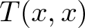 $T(x,x)$ and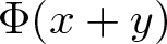 $\Phi (x+y)$ are hermitian.
(iii) For 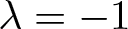 $\lambda =-1$, we have quaternions since we can extract $Y(x,y),V(x,y)$ from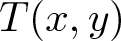 $T(x,y)$ and obtain a solution of the Gelfand–Levitan equation of the form
 \begin{align}0=&\begin{bmatrix} Y(x,y)&V(x,y)\\ -\overline{V}(x,y)&\overline{Y}(x,y)\end{bmatrix} +\begin{bmatrix} 0&\phi (x+y)\\ -\overline{\phi} (x+y) &0\end{bmatrix}\nonumber\\
&\quad +\int_x^\infty
\begin{bmatrix} Y(x,z)&V(x,z)\\ -\overline{V}(x,z)&\overline{Y}(x,z)\end{bmatrix}\begin{bmatrix} 0&\phi (z+y)\\ -\overline{\phi} (z+y)&0\end{bmatrix}\, dz,\end{align}
\begin{align}0=&\begin{bmatrix} Y(x,y)&V(x,y)\\ -\overline{V}(x,y)&\overline{Y}(x,y)\end{bmatrix} +\begin{bmatrix} 0&\phi (x+y)\\ -\overline{\phi} (x+y) &0\end{bmatrix}\nonumber\\
&\quad +\int_x^\infty
\begin{bmatrix} Y(x,z)&V(x,z)\\ -\overline{V}(x,z)&\overline{Y}(x,z)\end{bmatrix}\begin{bmatrix} 0&\phi (z+y)\\ -\overline{\phi} (z+y)&0\end{bmatrix}\, dz,\end{align}so that the integral equation may be expressed in terms of quaternion units
 \begin{equation*} \Phi (x+y)=\mathop{{\rm Re}} \Phi (x+y)\begin{bmatrix} 0&1\\ -1&0\end{bmatrix} +\mathop{{\rm Im}} \Phi (x+y)\begin{bmatrix} 0&i\\ i&0\end{bmatrix}\end{equation*}
 \begin{align}T(x,y)&=\mathop{{\rm Re}} Y(x,y) \begin{bmatrix} 1&0\\ 0&1\end{bmatrix}+\mathop{{\rm Im}} Y(x,y) \begin{bmatrix} i&0\\ 0&-i\end{bmatrix}\nonumber\\
&+\mathop{{\rm Re}} V(x,y) \begin{bmatrix} 0&1\\ -1&0\end{bmatrix}+\mathop{{\rm Im}} V(x,y) \begin{bmatrix} 0&i\\ i&0\end{bmatrix}.\end{align}
\begin{align}T(x,y)&=\mathop{{\rm Re}} Y(x,y) \begin{bmatrix} 1&0\\ 0&1\end{bmatrix}+\mathop{{\rm Im}} Y(x,y) \begin{bmatrix} i&0\\ 0&-i\end{bmatrix}\nonumber\\
&+\mathop{{\rm Re}} V(x,y) \begin{bmatrix} 0&1\\ -1&0\end{bmatrix}+\mathop{{\rm Im}} V(x,y) \begin{bmatrix} 0&i\\ i&0\end{bmatrix}.\end{align} Also  $U(x)=-2{\frac{d}{dx}} T(x,x)$ is a quaternion; hence, the noncommutative differential ring generated by $U(x)$ with differential $d/dx$ is a subring of $C^\infty ((0, \infty );{\mathbb H} )$. We have quaternions
 \begin{equation*} U=-4\lfloor \hat A\rfloor,\quad {\frac{d^jU}{dx^j}}=-4\lfloor D^j_x\hat A\rfloor ,\quad U^j=(-4)^j \lfloor \hat A\ast\dots \ast \hat A\rfloor .\end{equation*}
5. Spectra of Hankel operators associated with ZS
Under the hypotheses of (ii) and (iii) of Proposition 4.6, we consider
 \begin{equation*}(ii)\quad \Phi (x)=\begin{bmatrix} 0&\phi (x)\\ \overline{\phi (x)}&0\end{bmatrix} ,\qquad (iii) \quad \Psi (x)=\begin{bmatrix} 0&i\phi (x)\\ -i\overline{\phi (x)} &0\end{bmatrix}.\end{equation*}
 By the spectral theorem [Reference Birman and Solomjak3, p 177], a bounded and self-adjoint operator  $\Gamma$ on a separable Hilbert space $H$ has a resolution $H=\int^\oplus H(t)\mu (dt)$ where $\mu$ is a positive Radon measure on ${\mathbb R}$ called the scalar spectral measure or maximal spectral type and $\Gamma h(t)=th(t)$ where $h(t)\in H(t)$. The spectral multiplicity is $\nu :{\mathbb R}\rightarrow {\mathbb N}\cup \{\infty \}$ with $\nu (t)=\dim H(t)$. In particular, let $\mathop{\mathrm{null}} (\Gamma )=\{\xi\in H:\Gamma \xi =0\}$.
Proposition 5.1. Then  $\Gamma_\Phi$ gives a bounded and self-adjoint operator on $L^2((0, \infty ); {\mathbb C}^{2\times 1})$ with scalar spectral measure $\mu$. Let $\mu=\mu_a+\mu_s$ be the Lebesgue decomposition into an absolutely continuous measure $\mu_a$ and a singular measure $\mu_s$ with respect to Lebesgue measure. Then the spectral multiplicity function $\nu$ satisfies
(i) either
$\mathop{\mathrm{null}} (\Gamma_\Phi )=\{0\}$, or
$\dim \mathop{\mathrm{null}} (\Gamma_\Phi )=\infty$;(ii)
$\Gamma_\Phi $ is not invertible;(iii)
$\nu (t)=\nu (-t)$ for all
$t \gt 0$.





A similar statement holds for  $\Gamma_\Psi$ with obvious changes.
Proof. Recall the Laguerre polynomials  $L_n(t)={\frac{e^t}{n!}} {\frac{d^n}{dt^n}}(t^ne^{-t})$, so $(e^{-t/2}L_n(t))_{n=0}^\infty$ gives a complete orthonormal basis of $L^2((0, \infty ); {\mathbb C} )$. We introduce
 \begin{equation*}\gamma_n=\sqrt{2}\int_0^\infty \Phi (x)L_n(2x)e^{-x}\, dx,\end{equation*}
which are  $2\times2$ self-adjoint matrices for $n=0, 1, \dots$. Then the Hankel integral operator $\Gamma_\Phi$ on $L^2((0, \infty ); {\mathbb C}^{2\times 1})$ is unitarily equivalent to the self-adjoint block-Hankel matrix $\Gamma=[\gamma_{n+m}]_{n,m=0}^\infty$ on $\ell^2({\mathbb C}^{2\times 1})$. Now we apply Theorem 2 of [Reference Megretski, Peller and Treil49], which gives (i), (ii) and the balance conditions for multiplicity of absolutely continuous and singular spectra
 \begin{align}\vert\nu (t)-\nu (-t)\vert \leq 4&\quad {\hbox{for}}\quad \mu_a\quad{\hbox {almost all}}\quad t;\nonumber\\
\vert \nu (t)-\nu (-t)\vert\leq 2&\quad {\hbox{for}}\quad \mu_s\quad {\hbox{almost all}}\quad t.\end{align}
\begin{align}\vert\nu (t)-\nu (-t)\vert \leq 4&\quad {\hbox{for}}\quad \mu_a\quad{\hbox {almost all}}\quad t;\nonumber\\
\vert \nu (t)-\nu (-t)\vert\leq 2&\quad {\hbox{for}}\quad \mu_s\quad {\hbox{almost all}}\quad t.\end{align} To sharpen this, we suppose that  $\eta\in L^2((0, \infty ); {\mathbb C} )$ is an eigenvector of $\Gamma_\phi^\dagger \Gamma_\phi$, so $\Gamma_\phi^\dagger\Gamma_\phi \eta =s^2\eta$ for some $s \gt 0$; then
 \begin{equation} \begin{bmatrix} 0&\Gamma_\phi \\ \Gamma_\phi^\dagger&0\end{bmatrix} \begin{bmatrix}s^{-1}\Gamma_\phi \eta \\ \eta \end{bmatrix} =s \begin{bmatrix}s^{-1}\Gamma_\phi \eta \\ \eta \end{bmatrix}; \end{equation}
likewise, when we replace  $s$ by $-s$, so eigenvalues arise in pairs of opposite sign. Hence, $\nu (t)=\nu (-t)$ for all $y$ in the support of the discrete part of $\mu_s$, namely the set of eigenvalues.
Since  $\Gamma_\Phi$ is self-adjoint, its spectrum coincides with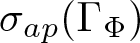 $\sigma_{ap}(\Gamma_\Phi)$; likewise for $\Gamma_\phi^\dagger\Gamma_\phi$. Let $(\eta_j)$ be an approximate eigenvector for $\Gamma_\phi^\dagger\Gamma_\phi$ with approximate eigenvalue $\lambda \gt 0$, so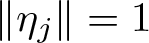 $\Vert \eta_j\Vert =1$ and $\Vert \Gamma_\phi^\dagger \Gamma_\phi \eta_j-\lambda\eta_j\Vert\rightarrow 0$ as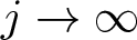 $j\rightarrow\infty$; then $[\Gamma_\phi \eta_j /\sqrt{\lambda}; \eta_j ]^\top$ gives an approximate eigenvector of $\Gamma_\Phi$ corresponding to approximate eigenvalue $\sqrt{\lambda}$ as in (5.2); conversely, approximate eigenvectors for $\Gamma_\Phi$ with approximate eigenvalue $s \gt 0$ gives an approximate eigenvector for $\Gamma_\phi^\dagger\Gamma_\phi$ with approximate eigenvalue $s^2$. This suggests that
 \begin{equation*} \nu_{\Gamma_\phi^\dagger \Gamma_\phi} (\lambda )=\nu_{\Gamma_\Phi}\bigl(\sqrt{\lambda}\bigr)=\nu_{\Gamma_\Phi}\bigl(-\sqrt{\lambda }\bigr)\qquad (\lambda \gt 0),\end{equation*}
as in (iii). To make this precise, we introduce the Banach space ultrapower 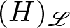 $(H)_\mathscr{L}$, which is essentially the quotient space $\ell^\infty ({\mathbb N}; H)/\mathcal{N}_\mathscr{L}$ where $\mathcal{N}_\mathscr{L}= \{(\xi_j)\in \ell^\infty ({\mathbb N} ;H): \mathop{\mathrm{LIM}} \Vert \xi_j\Vert =0\}$ and $\mathop{\mathrm{LIM}}$ is a Banach limit on ${\mathbb N}$. Then by a simple case of [Reference Heinrichs38, Theorem 3.3(ii)],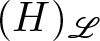 $(H)_\mathscr{L}$ is a Banach space that satisfies the parallelogram law, hence, is a Hilbert space. Let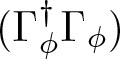 $(\Gamma_\phi^\dagger\Gamma_\phi )$ be the bounded linear operator on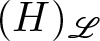 $(H)_\mathscr{L}$ that is determined by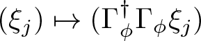 $(\xi_j)\mapsto (\Gamma_\phi^\dagger\Gamma_\phi \xi_j)$ for $(\xi_j)\in \ell^\infty ({\mathbb N} ;H)$. Then by the Gram-Schmidt process, one shows that $\nu_{\Gamma_\phi^\dagger\Gamma_\phi}(\lambda)=\dim\{\eta\in (H)_\mathscr{L}: (\Gamma_\phi^\dagger\Gamma_\phi)\eta =\lambda\eta\}$.
We have
 \begin{equation*} \Gamma_\Phi^2=\begin{bmatrix}\Gamma_\phi \Gamma_\phi^\dagger &0\\ 0&\Gamma_\phi^\dagger\Gamma_\phi\end{bmatrix}\end{equation*}
where  $\sigma (\Gamma_\phi\Gamma_\phi^\dagger )=\sigma (\Gamma_\phi^\dagger\Gamma_\phi )$ and there exist spectral families $K=\int^\oplus K(t)\mu (dt)$ for $\Gamma_\phi\Gamma_\phi^\dagger$ and $G=\int^\oplus G(t)\omega (dt)$ for $\Gamma_\phi^\dagger \Gamma_\phi$ where $\mu$ and $\omega$ are positive measures on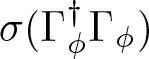 $\sigma (\Gamma_\phi^\dagger\Gamma_\phi )$. Then by the Radon–Nikodym theorem, we can introduce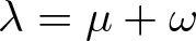 $\lambda =\mu+\omega$ and $\lambda$-measurable functions $k,g$ such that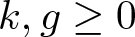 $k,g\geq 0$ and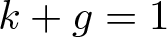 $k+g=1$ such that $\mu (dt)=k(t)\lambda (dt)$ and $\omega (dt)=g(t)\lambda (dt)$. Then let $H(t)=K(t)\oplus G(t)$ with the inner product
 \begin{equation*} \Bigl\langle \begin{bmatrix} k_1(t)\\ g_1(t)\end{bmatrix},\begin{bmatrix} k_2(t)\\ g_2(t)\end{bmatrix}\Bigr\rangle_{H(t)}=k(t)\langle k_1(t), k_2(t)\rangle_{K(t)}+g(t)\langle g_1(t), g_2(t)\rangle_{G(t)}.\end{equation*}
 Then  $H=\int^\oplus H(t)\lambda (dt)$ contains $K$ and $G$ as orthogonal subspaces, and $\Gamma_\Phi^2$ is unitarily equivalent to multiplication by $t$ on $H$.
$H$.
In the case of a nonnegative and self-adjoint compact Hankel operator, nonzero eigenvalues are all simple. This is in contrast to Proposition 5.1, as we have not proposed a bound on  $\nu (t)$. The decay rate of singular numbers is reflected in the asymptotics of the Fredholm determinant, as follows.
Proposition 5.2. Suppose that  $\Gamma_\phi$ is Hilbert–Schmidt, and let $s_0^2\geq s_1^2\geq \dots$ be the eigenvalues of $\Gamma_\phi^\dagger\Gamma_\phi$, listed according to multiplicity. Let $n(t)=\sharp \{j: ts_j^2\geq 1\}$.
(i) Then
$\det (I+ix\Gamma_\phi )$ is an entire and even function of
$x$.(ii) There exist
$\alpha, \beta \gt 0$ such that
$n(t)\sim \alpha t^\beta$ as
$t\rightarrow\infty$, if and only if
(5.3)\begin{equation} \log\det (I+ix\Gamma_\Phi )\sim \pi\alpha \mathop{\mathrm{cosec}} (\pi\beta ) x^{2\beta }\qquad (x\in (0, \infty ), x\rightarrow\infty ).\end{equation}


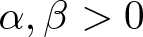
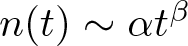
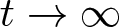

Proof. (i) We have a standard summation formula
 \begin{align}
\log\det (I+ix\Gamma_\Phi )&=\log\det (I+x^2\Gamma_\phi^\dagger \Gamma_\phi)\nonumber\\
&=\log\prod_{j=0}^\infty (1+x^2s_j^2)\nonumber\\
&=x^2\int_0^\infty {\frac {n(t)\, dt}{t(t+x^2)}}\qquad (x^2\in {\mathbb C}\setminus (0, \infty )).
\end{align}
\begin{align}
\log\det (I+ix\Gamma_\Phi )&=\log\det (I+x^2\Gamma_\phi^\dagger \Gamma_\phi)\nonumber\\
&=\log\prod_{j=0}^\infty (1+x^2s_j^2)\nonumber\\
&=x^2\int_0^\infty {\frac {n(t)\, dt}{t(t+x^2)}}\qquad (x^2\in {\mathbb C}\setminus (0, \infty )).
\end{align}The product converges, hence, we have an entire function.
(ii) If 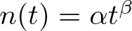 $n(t)=\alpha t^\beta$, then one can substitute $t=x^2\tan\theta$ and reduce the integral to $\alpha \Gamma (\beta )\Gamma (1-\beta )x^{2\beta}$, where here $\Gamma$ is Euler’s gamma function. By an approximation argument from [Reference Titchmarsh67, p 271], one obtains a corresponding asymptotic formula when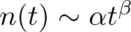 $n(t)\sim \alpha t^{\beta}$ and $x\rightarrow\infty$ through real values. The converse also holds, by a Tauberian theorem due to Valiron [Reference Valiron68, (58), p.237] . See also [Reference Blower5, Theorem 6.1] for conditions on $\phi$ that ensure rapid convergence of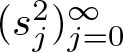 $(s_j^2)_{j=0}^\infty$.
6. Integral equations relating to KP
We start by introducing families of linear systems and related operators, and obtain a determinant formula which we then express in more classical terms. Let  $(-A, B(\zeta ),C)$ be a one-parameter family of continuous-time linear systems with state space $H$ and input and output space $H_1$. Let $\Phi (z,\zeta )=Ce^{-zA}B(\zeta )$ be the impulse response function and $R_x=\int_x^\infty B(\zeta )Ce^{-\zeta A}\, d\zeta$ as in (1.3) these are our basic operator functions, from which we introduce various auxiliary functions. Let $\Theta_x:L^2((0,\infty );H_1)\rightarrow H$ and $\Xi_x: L^2((0,\infty );H_1)\rightarrow H$ be defined by
 \begin{equation} \Theta_xh=\int_x^\infty e^{-\zeta A^\dagger}C^\dagger h(\zeta )d\zeta,\end{equation}
and
 \begin{equation} \Xi_x h=\int_x^\infty B(\zeta )h(\zeta ) \, d\zeta\qquad (h\in L^2((0, \infty ); H_1)) \end{equation}
and one computes  $\Theta^\dagger_x :H\rightarrow L^2((0, \infty ); H_1)$
 \begin{equation}\Theta^\dagger_x\alpha ={\mathbb I}_{(x, \infty )}(\zeta ) Ce^{-\zeta A}\alpha\qquad (\alpha\in H)\end{equation}
Hence
 \begin{align}\Theta^\dagger_x \Xi_x h&={\mathbb I}_{(x,\infty )}(z )Ce^{-zA} \int_x^\infty B(\zeta )h(\zeta )\, d\zeta \nonumber\\
&=\int_0^\infty {\mathbb I}_{(x,\infty )}(z)\Phi (z,\zeta ){\mathbb I}_{(x,\infty )}(\zeta )h(\zeta )d\zeta \qquad (h\in L^2((0, \infty );H_1),\end{align}
\begin{align}\Theta^\dagger_x \Xi_x h&={\mathbb I}_{(x,\infty )}(z )Ce^{-zA} \int_x^\infty B(\zeta )h(\zeta )\, d\zeta \nonumber\\
&=\int_0^\infty {\mathbb I}_{(x,\infty )}(z)\Phi (z,\zeta ){\mathbb I}_{(x,\infty )}(\zeta )h(\zeta )d\zeta \qquad (h\in L^2((0, \infty );H_1),\end{align}so  $\Theta^\dagger_0\Xi_0$ is the integral operator on $L^2((0, \infty );H_1)$ that has kernel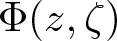 $\Phi (z, \zeta )$; while
 \begin{align}\Xi_x\Theta^\dagger_x\alpha &=\int_x^\infty
{\mathbb I}_{(x,\infty)}(\zeta )B(\zeta )Ce^{-\zeta A}\alpha \, d\zeta \nonumber\\
&=R_x\alpha \qquad (\alpha\in H),\end{align}
\begin{align}\Xi_x\Theta^\dagger_x\alpha &=\int_x^\infty
{\mathbb I}_{(x,\infty)}(\zeta )B(\zeta )Ce^{-\zeta A}\alpha \, d\zeta \nonumber\\
&=R_x\alpha \qquad (\alpha\in H),\end{align}which is our other basic operator. Next, we let
 \begin{equation} K(z, \zeta )=-Ce^{-zA}(I+R_z)^{-1}B(\zeta )\qquad (0 \lt z \lt \zeta )\end{equation}
which determines a Volterra-type integral operator
 \begin{equation} h\mapsto h(z)+\int_z^\infty K(z, \zeta )h(\zeta )\, d\zeta \qquad (h\in L^2((0, \infty );H_1).\end{equation}
Proposition 6.1. Suppose that  $\Theta_0$ and $\Xi_0$ are Hilbert–Schmidt, and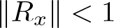 $\Vert R_x\Vert \lt 1$ for all $x \gt 0$.
(i) Then the Gelfand–Levitan equation
(6.8)is satisfied;\begin{equation} \Phi (z, \zeta )+K(z, \zeta )+\int_z^\infty K(z, \eta )\Phi (\eta , \zeta ) d\eta =0\end{equation}(ii) the operator
$\Theta_x^\dagger\Xi_x$ is trace class and may be expressed as the integral operator on
$L^2((0, \infty );H_1)$ that has kernel
$\Phi (x+z, x+\zeta )$;(iii) for
$H_1=\mathbb{C}$, the Fredholm determinant satisfies
(6.9)\begin{equation} {\frac{d}{dx}}\log\det (I+\Theta^\dagger_x \Xi_x)=K(x,x)\qquad (x \gt 0).\end{equation}




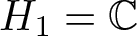

Proof. (i) Here, 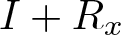 $I+R_x$ is invertible in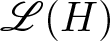 $\mathscr{L}(H)$, so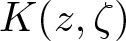 $K(z, \zeta )$ is defined. Then one verifies the Gelfand–Levitan equation by substitution. See [Reference Blower6, Lemma 5.1].
(ii) The operator  $\Theta_0^\dagger\Xi_0$ is a product of Hilbert–Schmidt operators, hence, trace class, and has compression $\Theta_x^\dagger\Xi_x$, which is also trace class.
(iii) We have
 \begin{equation} \det (I+\Theta_x^\dagger \Xi_x)=\det (I+\Xi_x\Theta^\dagger_x)=\det(I+R_x)\end{equation}
so
 \begin{align}{\frac{d}{dx}}\log\det (I+\Theta_x^\dagger\Xi_x)&={\frac{d}{dx}}{\hbox{trace}}\log (I+R_x)\nonumber\\
&={\hbox{trace}} \Bigl( (I+R_x)^{-1}{\frac{d}{dx}} R_x\Bigr)\nonumber\\
&=-{\hbox{trace}}\bigl( (I+R_x)^{-1} B(x)Ce^{-xA}\bigr)\nonumber\\
&=-{\hbox{trace}}\bigl( Ce^{-xA}(I+R_x)^{-1}B(x)\bigr)\nonumber\\
&={\hbox{trace}}\, K(x,x).\end{align}
\begin{align}{\frac{d}{dx}}\log\det (I+\Theta_x^\dagger\Xi_x)&={\frac{d}{dx}}{\hbox{trace}}\log (I+R_x)\nonumber\\
&={\hbox{trace}} \Bigl( (I+R_x)^{-1}{\frac{d}{dx}} R_x\Bigr)\nonumber\\
&=-{\hbox{trace}}\bigl( (I+R_x)^{-1} B(x)Ce^{-xA}\bigr)\nonumber\\
&=-{\hbox{trace}}\bigl( Ce^{-xA}(I+R_x)^{-1}B(x)\bigr)\nonumber\\
&={\hbox{trace}}\, K(x,x).\end{align} For 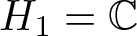 $H_1=\mathbb{C}$, we have $K(x,x)={\hbox{trace}}\, K(x,x)$.
Squares of Hankel operators are themselves associated with tau functions, and on account of Theorem 2.4(iv) can be simpler to use in computations than Hankel operators. For a specific example relating to Painlevé equation and concentric  $KdV$, see [Reference Drazin and Johnson27, p. 172]. In [Reference Blower and Doust9, Section 4], we discussed a differential ring related to the Hastings–McLeod solution of Painlevé II and obtained the following determinant from a Hankel square operator in [Reference Blower and Doust9, Proposition 4.1(ii)] and Example 9.2. The values of $\det (I\pm R_x)$ are equivalent data to the values of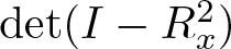 $\det (I-R_x^2)$ and $\det ((I+R_x)(I-R_x)^{-1})$ for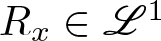 $R_x\in\mathscr{L}^1$ such that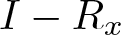 $I-R_x$ is invertible.
Proposition 6.2. Let 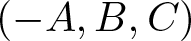 $(-A,B,C)$ be admissible, and introduce
 \begin{equation*} F(x,z)=\int_0^\infty \phi (x+y)\phi (y+z)\, dy.\end{equation*}
Then the integral equation
 \begin{equation} K(x,z)+\kappa F(x,z)+\kappa \int_x^\infty K(x,y)F(y,z)\, dy=0\end{equation}
has solution
 \begin{equation*} K(x,z)=-\kappa Ce^{-xA}(I+\kappa R_xR_0)^{-1}R_0e^{-zA}B,\end{equation*}
where
 \begin{equation*} K(x,x)={\frac{d}{dx}}\log\det (I+\kappa R_{x/2}^2).\end{equation*}
Proof. One can verify (6.12), starting from the formula  $F(x,z)=Ce^{-xA}R_0e^{-zA}B$. The determinant formula
 \begin{equation*} K(x,x)={\frac{d}{dx}}\log\det (I+\kappa R_xR_0)\end{equation*}
follows as in Lemma 2.8, and we have
 \begin{align}
\det \bigl(I+\kappa R_xR_0\bigr)&=\det \bigl(I+e^{-xA}R_0e^{-xA}R_0\bigr)\nonumber\\
&=\det \bigl(I+\kappa e^{-xA/2}R_0e^{-xA}R_0e^{-xA/2}\bigr)\nonumber\\
&=\det \bigl(I+\kappa R_{x/2}^2\bigr).
\end{align}
\begin{align}
\det \bigl(I+\kappa R_xR_0\bigr)&=\det \bigl(I+e^{-xA}R_0e^{-xA}R_0\bigr)\nonumber\\
&=\det \bigl(I+\kappa e^{-xA/2}R_0e^{-xA}R_0e^{-xA/2}\bigr)\nonumber\\
&=\det \bigl(I+\kappa R_{x/2}^2\bigr).
\end{align}Example 6.3. Consider the differential operator
 \begin{equation}L_0\psi =-{\frac{d^2\psi }{dx^2}}+\beta \psi\qquad (\psi \in C_c^\infty ((0, \infty ); \mathbb{C}))\end{equation}
which is semibounded for 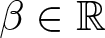 $\beta \in \mathbb{R}$ and positive for all $\beta \gt 0$. Suppose for simplicity that $\beta\geq 0$.
Here, we choose the continuous-time linear systems  $(-A,B(\zeta ),C)$ with state space $H=L^2((0, \infty ); \mathbb{C}^{2\times 1})$ and input and output space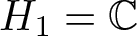 $H_1=\mathbb{C}$ with operators
 \begin{align}
-A&=\begin{bmatrix}0&-I\\ L_0&0\end{bmatrix}, \nonumber\\
B(\zeta )\alpha &=\begin{bmatrix} f(t+\zeta )\\ g(t+\zeta )\end{bmatrix}\alpha ,\nonumber\\
C:\begin{bmatrix} h_1(t)\\ h_2(t)\end{bmatrix} &\mapsto h_1(0)\qquad (h_1\in H^1((0,\infty );\mathbb{C})).
\end{align}
\begin{align}
-A&=\begin{bmatrix}0&-I\\ L_0&0\end{bmatrix}, \nonumber\\
B(\zeta )\alpha &=\begin{bmatrix} f(t+\zeta )\\ g(t+\zeta )\end{bmatrix}\alpha ,\nonumber\\
C:\begin{bmatrix} h_1(t)\\ h_2(t)\end{bmatrix} &\mapsto h_1(0)\qquad (h_1\in H^1((0,\infty );\mathbb{C})).
\end{align} Note that  $f(t)\mapsto f(t+\zeta )$ is the backward shift operator, which is strongly continuous and unitary on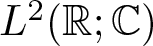 $L^2(\mathbb{R}; \mathbb{C})$ and strongly continuous and coisometric on $L^2((0, \infty ); \mathbb{C})$. Then $CB(\zeta )=f(\zeta )$, and the impulse response function is
 \begin{equation}\Phi (z, \zeta )=Ce^{-zA}B(\zeta )= \psi (z,\zeta ).\end{equation}
 Next we provide an explicit expression for this solution in classical style. We use spatial coordinates 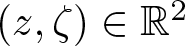 $(z, \zeta )\in \mathbb{R}^2$, variables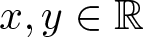 $x,y\in\mathbb{R}$, a spectral parameter $\kappa\in {\mathbb{R}}\cup i{\mathbb{R}}$ for an operator in $(z, \zeta )$, and a Fourier transform variable $\omega$ which is dual to $y$.
$y$.
We show how to obtain 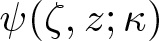 $\psi (\zeta ,z;\kappa )$ that is a solution of the system
 \begin{align}
{\frac{\partial^2\psi}{\partial \zeta ^2}}-{\frac{\partial^2\psi }{\partial z^2}} &+\kappa^2\psi =0\nonumber\\
\psi (\zeta ,0;\kappa )&=f(\zeta ;\kappa )\nonumber\\
{\frac{\partial\psi }{\partial z}}(\zeta ,0;\kappa )&=g(\zeta ;\kappa ).
\end{align}
\begin{align}
{\frac{\partial^2\psi}{\partial \zeta ^2}}-{\frac{\partial^2\psi }{\partial z^2}} &+\kappa^2\psi =0\nonumber\\
\psi (\zeta ,0;\kappa )&=f(\zeta ;\kappa )\nonumber\\
{\frac{\partial\psi }{\partial z}}(\zeta ,0;\kappa )&=g(\zeta ;\kappa ).
\end{align} Let  $J_n$ be Bessel’s function of the first kind of order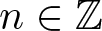 $n\in {\mathbb Z}$, defined by
 \begin{equation} J_n(x)=\int_0^{\pi} \cos\bigl(n\theta -x\sin\theta \bigr) {\frac{d\theta}{\pi}}\qquad (x\in{\mathbb C}) \end{equation}
and let  $K_0$ be the modified Bessel function of the second kind
 \begin{equation}K_0(w)=\int_0^\infty e^{-w\cosh t}\, dt\qquad (w\in {\mathbb C} )\end{equation}
such that  $K_0(w)=J_0(iw)$.
Lemma 6.4. Let
 \begin{align}\psi (\zeta ,z;\kappa )=&{\frac{1}{2}}\Bigl( f(\zeta +z;\kappa )+f(\zeta -z;\kappa )+{\frac{1}{2}}\int_{\zeta -z}^{\zeta +z} g(\xi ;\kappa )J_0\bigl(\kappa \sqrt{(\xi -\zeta )^2-z^2}\bigr)\, d\xi\nonumber\\
{}&\quad +\kappa^2z\int_{\zeta -z}^{\zeta +z} f(\xi ;\kappa ){\frac{J_0'( \kappa \sqrt{(\xi -\zeta )^2-z^2})}{\sqrt{(\xi -\zeta )^2-z^2}}} \, d\xi .\end{align}
\begin{align}\psi (\zeta ,z;\kappa )=&{\frac{1}{2}}\Bigl( f(\zeta +z;\kappa )+f(\zeta -z;\kappa )+{\frac{1}{2}}\int_{\zeta -z}^{\zeta +z} g(\xi ;\kappa )J_0\bigl(\kappa \sqrt{(\xi -\zeta )^2-z^2}\bigr)\, d\xi\nonumber\\
{}&\quad +\kappa^2z\int_{\zeta -z}^{\zeta +z} f(\xi ;\kappa ){\frac{J_0'( \kappa \sqrt{(\xi -\zeta )^2-z^2})}{\sqrt{(\xi -\zeta )^2-z^2}}} \, d\xi .\end{align}(i) Then
$\psi$ satisfies the system (6.17).(ii) For
$\beta=0$, the differential equation in (6.17) reduces to the wave equation, and the solution is given by
(6.21)\begin{equation} \psi (\zeta ,z;0) ={\frac{1}{2}} \Bigl( f(\zeta -z;0)+f(\zeta +z;0)\Bigr) +{\frac{1}{2}}\int_{\zeta -z}^{\zeta +z} g(\xi ;0)\, d\xi .\end{equation}


Proof. (i) Observe that  $G(x,y)=J_0(\sqrt{(x-\xi )(y-\eta )})$ satisfies
 \begin{equation} {\frac{\partial^2G}{\partial x\partial y}}=-{\frac{1}{4}} G(x,y).\end{equation}
 Then by the Riemann-Volterra method for the wave equation, as in [Reference Sneddon66] page 226, a solution to the preceding system is given by (6.17). To change from 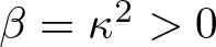 $\beta =\kappa^2 \gt 0$ to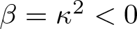 $\beta=\kappa^2 \lt 0$, we replace
 \begin{equation}J_0\bigl(\kappa\sqrt{(\xi -\zeta )^2-z^2}\bigr)=K_0\bigl(\kappa\sqrt{z^2-(\xi -\zeta )^2}\bigr) .\end{equation}
 To interpret this formula geometrically, we make a change of variables  $z=u+v$ and $\xi-\zeta=2\sqrt{uv}\cos t$. Then $z^2-(\xi-\zeta )^2= u^2+v^2-2uv\cos t$, as in the cosine formula for plane trigonometry, so
 \begin{equation} J_0(\lambda u)J_0(\lambda v)=\int_0^{2\pi} J_0\bigl(\lambda \sqrt{u^2+v^2-2uv\cos t}\Bigr) {\frac{dt}{2\pi}}.\end{equation}
 (ii) For 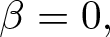 $\beta =0,$ we have the wave equation, and the stated solution is a particular case of D’Alembert’s formula.
We return to general 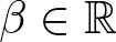 $\beta\in \mathbb{R}$, and observe that
 \begin{equation} \Phi (z, \zeta y;\kappa)=\psi (z, \zeta ;\kappa )e^{-\kappa^2y}\end{equation}
as a function of  $y$ is the Fourier transform in the $\omega$-variable of
 \begin{equation}\check{\Phi} (z,\zeta, \omega; \kappa )={\frac{\kappa^2}{\pi}}{\frac{\psi (z,\zeta; \kappa)}{\omega^2+\kappa^4}}\end{equation}
Then the Gelfand–Levitan equation
 \begin{equation}0=\check{\Phi}(z, \zeta ,\omega ;\kappa)+\check{K}(z, \zeta ,\omega ;\kappa )+\int_z^\infty \int_{-\infty}^\infty \check{K}(z, \eta ,\omega-\nu ; \kappa )\check{\Phi} (\eta, \zeta, \nu ;\kappa )d\nu d\eta \end{equation}
has Fourier transform
 \begin{equation}0={\Phi}(z, \zeta ,y;\kappa )+{K}(z, \zeta ,y;\kappa )+\int_z^\infty {K}(z, \eta ,y; \kappa ){\Phi} (\eta, \zeta, y ;\kappa )d\eta , \end{equation}
and we can solve this as above. Suppose that  $c:(a_1, a_2)\rightarrow \mathbb{C}$ is an integrable function and
 \begin{equation}\Phi (z,\zeta ,y)=\int_{a_1}^{a_2} e^{\kappa^2y}c(\kappa )\psi (z, \zeta ;\kappa )\, d\kappa .\end{equation}
 Here, we choose the continuous-time linear systems  $(-A,B(\zeta ),C)$ with state space $H=L^2((0, \infty )\times (a_1,a_2); \mathbb{C}^{2\times 1})$ and input and output space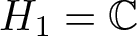 $H_1=\mathbb{C}$ with operators
 \begin{align}
-A&=\begin{bmatrix}0&-I\\ L_0&0\end{bmatrix};\nonumber\\
B(\zeta )\alpha &=\begin{bmatrix} f(t+\zeta ;\kappa )\\ g(t+\zeta ;\kappa )\end{bmatrix}\alpha \qquad (\alpha\in \mathbb{C});\nonumber\\
C:\begin{bmatrix} h_1(t,\kappa )\\ h_2(t,\kappa )\end{bmatrix} &\mapsto \int_{a_1}^{a_2} c(\kappa )h_1(0,\kappa )\, d\kappa\qquad (h_1\in H^1((0,\infty );L^2(a_1,a_2);\mathbb{C}))).
\end{align}
\begin{align}
-A&=\begin{bmatrix}0&-I\\ L_0&0\end{bmatrix};\nonumber\\
B(\zeta )\alpha &=\begin{bmatrix} f(t+\zeta ;\kappa )\\ g(t+\zeta ;\kappa )\end{bmatrix}\alpha \qquad (\alpha\in \mathbb{C});\nonumber\\
C:\begin{bmatrix} h_1(t,\kappa )\\ h_2(t,\kappa )\end{bmatrix} &\mapsto \int_{a_1}^{a_2} c(\kappa )h_1(0,\kappa )\, d\kappa\qquad (h_1\in H^1((0,\infty );L^2(a_1,a_2);\mathbb{C}))).
\end{align}Proposition 6.5. Let 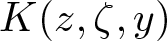 $K(z,\zeta ,y)$ be the solution of the Gelfand–Levitan equation (6.36) that corresponds (6.30), and let
 \begin{equation} u(z;y)=-2{\frac{d}{dz}} K(z,z,y).\end{equation}
Then
 \begin{equation}u(z;y)=-2{\frac{d^2}{dz^2}}\log\det (I+\Theta_z^\dagger\Xi_z)\end{equation}
and
 \begin{equation}\beta {\frac{\partial K}{\partial y}}(z,\zeta ,y)+{\frac{\partial^2K}{\partial z^2}}(z,\zeta ,y)-{\frac{\partial^2K}{\partial \zeta^2}}(z,\zeta ,y)=u(z,y) K(z,\zeta ,y).\end{equation}
Proof. The impulse response function for the linear system is
 \begin{equation}\Phi (z, \zeta ,y)=Ce^{-zA}B(\zeta )= \int_{a_1}^{a_2}e^{\kappa^2y}\psi (z,\zeta ;\kappa )c(\kappa )\, d\kappa .\end{equation}
Hence, we have
 \begin{equation} \beta {\frac{\partial\Phi}{\partial y}}(z,\zeta ,y)+{\frac{\partial^2\Phi}{\partial z^2}}(z,\zeta ,y)-{\frac{\partial^2\Phi}{\partial \zeta^2}}(z,\zeta ,y)=0\end{equation}
and
 \begin{equation} \Phi (z,\zeta ,y)+K(z,\zeta ,y)+\int_z^\infty K(z,\eta ,y)\Phi (\eta ,\zeta ,y)\, d\eta =0\end{equation}
which together imply that
 \begin{align}-2&{\frac{d}{dz}}K(z,z,y) \Phi (z,\zeta ,y)+
\beta {\frac{\partial K}{\partial y}}(z,\zeta ,y)+{\frac{\partial^2K}{\partial z^2}}(z,\zeta ,y)-{\frac{\partial^2K}{\partial \zeta^2}}(z,\zeta ,y)\nonumber\\
&+\int_z^\infty \Bigl(\beta {\frac{\partial K}{\partial y}}(z,\eta ,y)+{\frac{\partial^2K}{\partial z^2}}(z,\eta ,y)-{\frac{\partial^2K}{\partial \eta^2}}(z,\eta ,y)\Bigr) \Phi (\eta, \zeta ,y)\, d\eta =0,\end{align}
\begin{align}-2&{\frac{d}{dz}}K(z,z,y) \Phi (z,\zeta ,y)+
\beta {\frac{\partial K}{\partial y}}(z,\zeta ,y)+{\frac{\partial^2K}{\partial z^2}}(z,\zeta ,y)-{\frac{\partial^2K}{\partial \zeta^2}}(z,\zeta ,y)\nonumber\\
&+\int_z^\infty \Bigl(\beta {\frac{\partial K}{\partial y}}(z,\eta ,y)+{\frac{\partial^2K}{\partial z^2}}(z,\eta ,y)-{\frac{\partial^2K}{\partial \eta^2}}(z,\eta ,y)\Bigr) \Phi (\eta, \zeta ,y)\, d\eta =0,\end{align}hence
 \begin{equation}\beta {\frac{\partial K}{\partial y}}(z,\zeta ,y)+{\frac{\partial^2K}{\partial z^2}}(z,\zeta ,y)-{\frac{\partial^2K}{\partial \zeta^2}}(z,\zeta ,y)=\Bigl(-2{\frac{d}{dz}}K(z,z,y) \Bigr)K(z,\zeta ,y).\end{equation}
Lemma 6.6. With
 \begin{equation}L_0=-\Bigl(\beta {\frac{\partial}{\partial y}}+{\frac{\partial^2}{\partial z^2}}\Bigr), \qquad
L_u=-\Bigl(\beta {\frac{\partial}{\partial y}}+{\frac{\partial^2}{\partial z^2}}\Bigr)+u(z,y),\end{equation}
\begin{equation}L_0=-\Bigl(\beta {\frac{\partial}{\partial y}}+{\frac{\partial^2}{\partial z^2}}\Bigr), \qquad
L_u=-\Bigl(\beta {\frac{\partial}{\partial y}}+{\frac{\partial^2}{\partial z^2}}\Bigr)+u(z,y),\end{equation}the Volterra-type operator 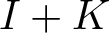 $I+K$ satisfies
 \begin{equation} L_u(I+K)=(I+K)L_0.\end{equation}
Proof. Let  $\theta =(I+K)\phi$, or more explicitly
 \begin{equation} \theta (z,y)=\phi (z,y)+\int_z^\infty K(z, \eta ,y)\phi (\eta ,y)\, d\eta;\end{equation}
then we have the identity
 \begin{align}\Bigl(\beta {\frac{\partial}{\partial y}}+{\frac{\partial^2}{\partial z^2}}\Bigr) \theta (z,y)&=\Bigl(\beta {\frac{\partial}{\partial y}}+{\frac{\partial^2}{\partial z^2}}\Bigr) \phi (z,y)+u(z)\int_z^\infty K(z,\eta ,y)\phi (\eta ,y)\, d\eta\nonumber\\
&\quad +\int_z^\infty K(z, \eta ,y) \Bigl(\beta {\frac{\partial}{\partial y}}+{\frac{\partial^2}{\partial \eta^2}}\Bigr) \phi (\eta ,y)\, d\eta .\end{align}
\begin{align}\Bigl(\beta {\frac{\partial}{\partial y}}+{\frac{\partial^2}{\partial z^2}}\Bigr) \theta (z,y)&=\Bigl(\beta {\frac{\partial}{\partial y}}+{\frac{\partial^2}{\partial z^2}}\Bigr) \phi (z,y)+u(z)\int_z^\infty K(z,\eta ,y)\phi (\eta ,y)\, d\eta\nonumber\\
&\quad +\int_z^\infty K(z, \eta ,y) \Bigl(\beta {\frac{\partial}{\partial y}}+{\frac{\partial^2}{\partial \eta^2}}\Bigr) \phi (\eta ,y)\, d\eta .\end{align}so  $L_u\theta =(I+K)L_0\phi$.
In particular, if
 \begin{equation}-\Bigl(\beta {\frac{\partial}{\partial y}}+{\frac{\partial^2}{\partial z^2}}\Bigr) \phi (z,y)=\kappa^2\phi (z,y),\end{equation}
then
 \begin{equation}-\Bigl(\beta {\frac{\partial}{\partial y}}+{\frac{\partial^2}{\partial z^2}}\Bigr) \theta (z,y)+u(z,y)\theta (z,y)=\kappa^2\phi (z,y).\end{equation}
7. A differential ring for KP
From  $\Phi$, we now obtain a solution of the linearized $KP$ equation in the standard form. We consider the semi-additive family of kernels
 \begin{equation} p(x,y,z,\zeta )=\Phi (z+x,\zeta +x; y)\end{equation}
such that
 \begin{equation} {\frac{\partial p}{\partial x}}={\frac{\partial p }{\partial z}}+{\frac{\partial p}{\partial \zeta }},\end{equation}
and
 \begin{equation}{\frac{\partial^2 p}{\partial z^2}}-{\frac{\partial^2 p}{\partial \zeta^2}}+\beta {\frac{\partial p}{\partial y}}=0.\end{equation}
 For each real  $x$, there is an operator $P_x$ given by
 \begin{equation} P_xh(y,z)=\int_{0}^\infty p(x,y,z,\zeta )h (y,\zeta )d\zeta \end{equation}
which is a multiplication operator as a function in the  $y$ variable and an integral operator in $\zeta$. Consider a family of linear systems $\Sigma_{(y,t)}=(-A, B(y), C(t))$ with impulse response function $\Phi (z, \zeta ; y,t)=C(t)e^{-(z+\zeta )A}B(y)$; then
 \begin{equation}R_{x;y,t}=\int_x^\infty e^{-\zeta A}B(y)C(t)e^{-\zeta A}\, d\zeta \end{equation}
gives
 \begin{equation}K(z,\zeta ;y,t)=-C(t)e^{-zA}(I+R_{z;y,t})^{-1}e^{-\zeta A}B(y)\end{equation}
which satisfies
 \begin{equation} \Phi (z+\zeta ;y,t)+K(z, \zeta ;y,t)+\int_z^\infty K(z, \eta ;y,t)\Phi (\eta +\zeta ;y,t)\, d\eta =0.\end{equation}
 We now introduce a version of the Pöppe bracket operation that is suited to the  $KP$ equation. The starting point is Lyapunov’s identity
 \begin{equation}{\frac{dR_{x;y,t}}{dx}}=-AR_{x;y,t}-R_{x;y,t}A=-e^{-zA}e^{-y\Delta}BCe^{-zA}.\end{equation}
Definition 7.1. Let  $\mathscr{A}$ be the complex algebra formed by linear combinations of products of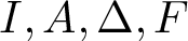 $I,A,\Delta ,F$, and let ${\frac{d}{dz}}$ and ${\frac{d}{dy}}$ be derivations on $\mathscr{A}$ such that
 \begin{equation}{\frac{dA}{dy}}={\frac{dA}{dz}}=0, \qquad{\frac{d\Delta}{dy}}={\frac{d\Delta}{dz}}=0,\end{equation}
 \begin{equation}{\frac{dF}{dx}}=AF+FA-2FAF, \qquad {\frac{dF}{dz}}=F\Delta (I-F).\end{equation}
 We also introduce the associative product  $\ast$ on ${\mathscr{A}}$ by
 \begin{equation} X\ast Y=X(AF+FA-2FAF)Y\end{equation}
and the differential expressions
 \begin{equation}D_zX=(A-2AF)X+{\frac{dX}{dz}} +X(A-2FA), \quad D_y X=\Delta (I-F)X +{\frac{dX}{dy}}-XF\Delta ;\end{equation}
the asymmetry here is intentional. Then we let
 \begin{equation} \lfloor X\rfloor = Ce^{-zA}F_zXF_ze^{-zA}e^{-y\Delta }B\qquad (y,z \gt 0).\end{equation}
Proposition 7.2. Suppose further that  $A\Delta=\Delta A.$ Then $({\mathscr{A}}, D_z,D_y, \ast )$ is a differential ring, and $\lfloor \cdot \rfloor$ is a differential ring homomorphism in the sense that
(i)
$\lfloor X\ast Y\rfloor =\lfloor X\rfloor \lfloor Y\rfloor$;(ii)
$ {\frac{d}{dz}}\lfloor X\rfloor =\lfloor D_zX\rfloor$;(iii)
${\frac{d}{dy}}\lfloor X\rfloor =\lfloor D_yX\rfloor$ for all
$X,Y\in {\mathscr{A}}$.



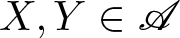
Proof. (i) This is a direct calculation as in [Reference Blower and Newsham13, Theorem 4.4] and the key step is at the right bracket  $\rfloor$, where $\ast$ is replaced by
 \begin{equation}AF_z+F_zA-2F_zAF_z={\frac{dF_z}{dz}}=F_ze^{-zA}e^{-y\Delta}BCe^{-zA}F_z.\end{equation}
 (ii) Note that at the left bracket  $\lfloor$ we have
 \begin{equation} {\frac{d}{dz}}Ce^{-zA}F=Ce^{-zA}\bigl( -AF+AF+FA-2FAF\bigr)=Ce^{-zA}F\bigl( A-2AF\bigr).\end{equation}
 (iii) At the right bracket  $\rfloor$ we have the $y$ derivative
 \begin{equation}{\frac{d}{dy}} Fe^{-zA}e^{-y\Delta}B= \bigl(F\Delta (I-F)-F\Delta \bigr)e^{-zA}e^{-y\Delta}B=-F\Delta Fe^{-zA}
e^{-y\Delta}B.\end{equation}
\begin{equation}{\frac{d}{dy}} Fe^{-zA}e^{-y\Delta}B= \bigl(F\Delta (I-F)-F\Delta \bigr)e^{-zA}e^{-y\Delta}B=-F\Delta Fe^{-zA}
e^{-y\Delta}B.\end{equation} For the family of linear systems  $(-A, e^{-y\Delta }B,C)$, we have
 \begin{equation}R_{z,y}=\int_z^\infty e^{-\zeta A}e^{-y\Delta}BCe^{-\zeta A}\, d\zeta,\end{equation}
then we define  $F_{z,y}=(I+R_{z,y})^{-1}$. Also, we have
 \begin{equation}\tau (z,y)=\det (I+R_{z,y}),\end{equation}
and
 \begin{equation}{\frac{\partial}{\partial z}}\log \tau (z,y)=K(z,z,y).\end{equation}
 Hence, the second-order partial derivatives of  $\log\tau$ satisfy
 \begin{align}u(z,y)&=-2{\frac{\partial K}{\partial z}}(z,z,y)=-4\lfloor A\rfloor \nonumber\\
w(z,y)&={\frac{-3\beta}{2}}{\frac{\partial K}{\partial y}}(z,z,y)={\frac{-3\beta}{2}}\lfloor \Delta \rfloor ,\end{align}
\begin{align}u(z,y)&=-2{\frac{\partial K}{\partial z}}(z,z,y)=-4\lfloor A\rfloor \nonumber\\
w(z,y)&={\frac{-3\beta}{2}}{\frac{\partial K}{\partial y}}(z,z,y)={\frac{-3\beta}{2}}\lfloor \Delta \rfloor ,\end{align}by calculations as in Proposition 7.2. With  $K(x,z)=-Ce^{-xA}(I+R_x)^{-1}e^{-zA}B$, we reconcile the brackets $[\cdot ]$ with $\lfloor\cdot \rfloor$, as in
 \begin{equation*} u(z,y)=-2{\frac{d}{dz}}\bigl[K\bigr]_{z,z}=2{\frac{d}{dz}}\bigl\lfloor I+R\bigr\rfloor_z=-4\bigl\lfloor A\rfloor_z.\end{equation*}
8. Solution of KP
Suppose that there is another parameter  $t$ such that
 \begin{equation}\alpha {\frac{\partial \Phi}{\partial t}}+{\frac{\partial^3\Phi}{\partial z^3}}+{\frac{\partial^3\Phi}{\partial \zeta^3}}=0.\end{equation}
 For the  $KP$ equation, we adjust the choice of $L_u$ to
 \begin{equation}L_0=-\Bigl(\beta {\frac{\partial}{\partial y}}+{\frac{\partial^2}{\partial z^2}}\Bigr), \qquad L_u=-\Bigl(\beta {\frac{\partial}{\partial y}}+{\frac{\partial^2}{\partial z^2}}\Bigr)+u(z,y,t)\end{equation}
to accommodate the extra variable  $t$, nevertheless, we have $L_u(I+K)=(I+K)L_0$, as in Lemma 6.6. As in (7.20), we define
 \begin{equation}w(z,y,t) ={\frac{-3\beta}{2}}{\frac{\partial K}{\partial y}}(z,z,y,t);\end{equation}
and recall that
 \begin{equation}u(z,y,t)=-2{\frac{\partial K}{\partial z}}(z,z,y,t).\end{equation}
Let
 \begin{equation}M_0 \theta =\alpha{\frac{\partial \theta}{\partial t}}+{\frac{\partial^3\theta}{\partial z^3}}, \end{equation}
 \begin{equation}M_u \theta =\alpha{\frac{\partial \theta}{\partial t}}+{\frac{\partial^3\theta}{\partial z^3}}-{\frac{3}{2}}u{\frac{\partial \theta}{\partial z}} -{\frac{3}{4}}{\frac{\partial u}{\partial z}}\theta +w\theta.\end{equation}
Proposition 8.1. The transformation  $X\mapsto (I+K)^{-1}X(I+K)$ takes the commuting pair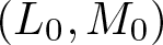 $(L_0,M_0)$ to a commuting pair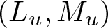 $(L_u,M_u)$, and $u$ satisfies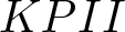 $KPII$.
Proof. From the integral equation,
 \begin{align}0=&{\frac{\partial\Phi}{\partial z}}(z,\zeta, y,t)+{\frac{\partial K}{\partial z}}(z, \zeta ,y,t)+\int_z^\infty{\frac{\partial K}{\partial z}}(z, \eta, y,t)\Phi (\eta, \zeta, y,t)\, d\eta\nonumber\\
&-K(z,z,y,t)\Phi (z,z,y,t),\end{align}
\begin{align}0=&{\frac{\partial\Phi}{\partial z}}(z,\zeta, y,t)+{\frac{\partial K}{\partial z}}(z, \zeta ,y,t)+\int_z^\infty{\frac{\partial K}{\partial z}}(z, \eta, y,t)\Phi (\eta, \zeta, y,t)\, d\eta\nonumber\\
&-K(z,z,y,t)\Phi (z,z,y,t),\end{align}and by calculating further derivatives, we find
 \begin{align}0=&\alpha {\frac{\partial\Phi}{\partial t}}(z,\zeta, y,t)+{\frac{\partial^3\Phi}{\partial z^3}}(z,\zeta, y,t)+ {\frac{\partial^3\Phi }{\partial \zeta^3}}(z, \zeta , y,t)\nonumber\\
&+ \alpha{\frac{\partial K}{\partial t}}(z,\zeta, y,t)+{\frac{\partial^3K}{\partial z^3}}(z,\zeta, y,t)+ {\frac{\partial^3K}{\partial \zeta^3}}(z, \zeta , y,t)\nonumber\\
&+\int_z^\infty \Bigl( \alpha{\frac{\partial K}{\partial t}}(z,\eta, y,t)+{\frac{\partial^3K}{\partial z^3}}(z,\eta, y,t)+ {\frac{\partial^3K }{\partial \eta^3}}(z, \eta , y,t)\Bigr) \Phi (\eta,\zeta, y,t)\, d\eta\nonumber\\
&+\Bigl( -2{\frac{d}{dz}}K(z,z,y,t)-{\frac{\partial K}{\partial z}}(z,z,y,t)-{\frac{\partial K}{\partial\zeta}}(z,z,y,t)\Bigr){\frac{\partial \Phi}{\partial z}}(z, \zeta ,y,t)\nonumber\\
&+\Bigl(-2{\frac{d^2K}{dz^2}}(z,z,y,t)-{\frac{d}{dz}}{\frac{\partial K}{\partial z}}(z,z,y,t)-{\frac{\partial^2K}{\partial z^2}}(z,z,y,t)+{\frac{\partial^2 K}{\partial \zeta^2}}(z,z,y,t)\Bigr)\nonumber\\
&\quad \Phi (z,\zeta ,y,t),\end{align}
\begin{align}0=&\alpha {\frac{\partial\Phi}{\partial t}}(z,\zeta, y,t)+{\frac{\partial^3\Phi}{\partial z^3}}(z,\zeta, y,t)+ {\frac{\partial^3\Phi }{\partial \zeta^3}}(z, \zeta , y,t)\nonumber\\
&+ \alpha{\frac{\partial K}{\partial t}}(z,\zeta, y,t)+{\frac{\partial^3K}{\partial z^3}}(z,\zeta, y,t)+ {\frac{\partial^3K}{\partial \zeta^3}}(z, \zeta , y,t)\nonumber\\
&+\int_z^\infty \Bigl( \alpha{\frac{\partial K}{\partial t}}(z,\eta, y,t)+{\frac{\partial^3K}{\partial z^3}}(z,\eta, y,t)+ {\frac{\partial^3K }{\partial \eta^3}}(z, \eta , y,t)\Bigr) \Phi (\eta,\zeta, y,t)\, d\eta\nonumber\\
&+\Bigl( -2{\frac{d}{dz}}K(z,z,y,t)-{\frac{\partial K}{\partial z}}(z,z,y,t)-{\frac{\partial K}{\partial\zeta}}(z,z,y,t)\Bigr){\frac{\partial \Phi}{\partial z}}(z, \zeta ,y,t)\nonumber\\
&+\Bigl(-2{\frac{d^2K}{dz^2}}(z,z,y,t)-{\frac{d}{dz}}{\frac{\partial K}{\partial z}}(z,z,y,t)-{\frac{\partial^2K}{\partial z^2}}(z,z,y,t)+{\frac{\partial^2 K}{\partial \zeta^2}}(z,z,y,t)\Bigr)\nonumber\\
&\quad \Phi (z,\zeta ,y,t),\end{align}where the coefficient of  $\Phi$ in the final line is
 \begin{align}{\frac{-3}{2}}&\Bigl( {\frac{\partial}{\partial z}}+{\frac{\partial}{\partial \zeta}}\Bigr)^2K(z,z,y,t)-{\frac{3}{2}}\Bigl( {\frac{\partial^2K}{\partial z^2}}(z,z,y,t)-{\frac{\partial^2K}{\partial\zeta^2}}(z,z,y,t)\Bigr)\nonumber\\
&={\frac{3}{4}}{\frac{\partial u}{\partial z}}(z,y,t)+ {\frac{3\beta}{2}}{\frac{\partial K}{\partial y}}(z,z,y,t)-{\frac{3}{2}}u(z,y,t)K(z,z,y,t),\end{align}
\begin{align}{\frac{-3}{2}}&\Bigl( {\frac{\partial}{\partial z}}+{\frac{\partial}{\partial \zeta}}\Bigr)^2K(z,z,y,t)-{\frac{3}{2}}\Bigl( {\frac{\partial^2K}{\partial z^2}}(z,z,y,t)-{\frac{\partial^2K}{\partial\zeta^2}}(z,z,y,t)\Bigr)\nonumber\\
&={\frac{3}{4}}{\frac{\partial u}{\partial z}}(z,y,t)+ {\frac{3\beta}{2}}{\frac{\partial K}{\partial y}}(z,z,y,t)-{\frac{3}{2}}u(z,y,t)K(z,z,y,t),\end{align}while the coefficient of  ${\frac{\partial \Phi}{\partial z}}$ in the preceding line is $(3/2)u(z,y,t)$ Then by adding $(3/2)u(z,y,t)$ times (8.7), we have
 \begin{align}0=&\alpha{\frac{\partial K}{\partial t}}(z,\zeta, y,t)+{\frac{\partial^3K}{\partial z^3}}(z,\zeta, y,t)+ {\frac{\partial^3K}{\partial \zeta^3}}(z, \zeta , y,t)-{\frac{3}{2}}u(z,y,t){\frac{\partial K}{\partial z}}(z,\zeta ,y,t)\nonumber\\
&+\Bigl( {\frac{3}{4}}{\frac{\partial u}{\partial z}}(z,y,t)+ {\frac{3\beta}{2}}{\frac{\partial K}{\partial y}}(z,z,y,t)\Bigr) \Phi (z, \zeta ,y,t)\nonumber\\
&+\int_z^\infty \Bigl( \alpha{\frac{\partial K}{\partial t}}(z,\eta, y,t)+{\frac{\partial^3K}{\partial z^3}}(z,\eta, y,t)+ {\frac{\partial^3K}{\partial \eta^3}}(z, \zeta , y,t)\nonumber\\
&\qquad -{\frac{3}{2}}u(z,y,t){\frac{\partial K}{\partial z}}(z,\eta ,y,t)\Bigr) \Phi (\eta, \zeta ,y,t)\, d\eta\end{align}
\begin{align}0=&\alpha{\frac{\partial K}{\partial t}}(z,\zeta, y,t)+{\frac{\partial^3K}{\partial z^3}}(z,\zeta, y,t)+ {\frac{\partial^3K}{\partial \zeta^3}}(z, \zeta , y,t)-{\frac{3}{2}}u(z,y,t){\frac{\partial K}{\partial z}}(z,\zeta ,y,t)\nonumber\\
&+\Bigl( {\frac{3}{4}}{\frac{\partial u}{\partial z}}(z,y,t)+ {\frac{3\beta}{2}}{\frac{\partial K}{\partial y}}(z,z,y,t)\Bigr) \Phi (z, \zeta ,y,t)\nonumber\\
&+\int_z^\infty \Bigl( \alpha{\frac{\partial K}{\partial t}}(z,\eta, y,t)+{\frac{\partial^3K}{\partial z^3}}(z,\eta, y,t)+ {\frac{\partial^3K}{\partial \eta^3}}(z, \zeta , y,t)\nonumber\\
&\qquad -{\frac{3}{2}}u(z,y,t){\frac{\partial K}{\partial z}}(z,\eta ,y,t)\Bigr) \Phi (\eta, \zeta ,y,t)\, d\eta\end{align}hence, we have the differential equation
 \begin{align}\Bigl( \alpha {\frac{\partial K}{\partial t}}+{\frac{\partial^3K}{\partial z^3}}&+{\frac{\partial^3 K}{\partial\zeta^3}}-{\frac{3}{2}} u{\frac{\partial K}{\partial z}}\Bigr)(z,\zeta, y,t)\nonumber\\
&={\frac{3}{4}}{\frac{\partial u}{\partial z}}K(z,\zeta, y,t)+{\frac{3\beta }{2}}{\frac{\partial K}{\partial y}}(z,z,y,t) K(z,\zeta ,y,t).\end{align}
\begin{align}\Bigl( \alpha {\frac{\partial K}{\partial t}}+{\frac{\partial^3K}{\partial z^3}}&+{\frac{\partial^3 K}{\partial\zeta^3}}-{\frac{3}{2}} u{\frac{\partial K}{\partial z}}\Bigr)(z,\zeta, y,t)\nonumber\\
&={\frac{3}{4}}{\frac{\partial u}{\partial z}}K(z,\zeta, y,t)+{\frac{3\beta }{2}}{\frac{\partial K}{\partial y}}(z,z,y,t) K(z,\zeta ,y,t).\end{align} The final term involves 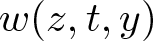 $w(z,t,y)$, which is so chosen that $M_u(I+K)=(I+K)M_0$, as one verifies by similar computations; hence,
 \begin{equation}[M_u,L_u](I+K)=(I+K)[M_0,L_0]\end{equation}
where  $M_0$ and $L_0$ have constant coefficients, hence
 \begin{equation}[M_u,L_u]=0\end{equation}
so  $L_u$ and $M_u$ commute. The condition on $w$ is that
 \begin{align}\beta {\frac{\partial w}{\partial y}}&=-{\frac{1}{4}}{\frac{\partial^3u}{\partial z^3}}+{\frac{3}{2}}u{\frac{\partial u}{\partial t}} -\alpha {\frac{\partial u}{\partial t}},\nonumber\\
{\frac{\partial w}{\partial z}}&={\frac{3\beta }{4}}{\frac{\partial u}{\partial y}}.\end{align}
\begin{align}\beta {\frac{\partial w}{\partial y}}&=-{\frac{1}{4}}{\frac{\partial^3u}{\partial z^3}}+{\frac{3}{2}}u{\frac{\partial u}{\partial t}} -\alpha {\frac{\partial u}{\partial t}},\nonumber\\
{\frac{\partial w}{\partial z}}&={\frac{3\beta }{4}}{\frac{\partial u}{\partial y}}.\end{align} The second of these follows from the choice of  $w$. The equality of mixed partials with
 \begin{equation}{\frac{\partial^2w}{\partial z\partial y}}={\frac{3\beta}{4}}{\frac{\partial^2u}{\partial y^2}}\end{equation}
is equivalent to the  $KP$ system of partial differential equations (1.1). We can also express this as an evolution equation
 \begin{equation}
\Bigl( \alpha{\frac{\partial u}{\partial t}}+{\frac{1}{4}}{\frac{\partial^3u}{\partial z^3}}-{\frac{3}{2}}u{\frac{\partial u}{\partial z}}\Bigr)+
\int{\frac{3\beta^2}{4}}{\frac{\partial^2u}{\partial y^2}}dz
=0;\end{equation}
\begin{equation}
\Bigl( \alpha{\frac{\partial u}{\partial t}}+{\frac{1}{4}}{\frac{\partial^3u}{\partial z^3}}-{\frac{3}{2}}u{\frac{\partial u}{\partial z}}\Bigr)+
\int{\frac{3\beta^2}{4}}{\frac{\partial^2u}{\partial y^2}}dz
=0;\end{equation}indeed, this is the form in which the equation is usually solved.
9. Examples and Remarks
In Propositions 4.5 and 8.1, we use a trace-class  $R_x$ that arises as the product of Hilbert–Schmidt operators. This is a more stringent hypothesis than admissibility, as in 4.1, so in this section, we give conditions for various linear systems to produce operators in trace ideals. Let $H=L^2(\mathbb{R}; \mathbb{C})$ and $\mathscr{D}(A)=\{f\in H: vf(v)\in H\}$, let ${\mathscr{D}}(\Delta )=\{f\in H: v^3f(v)\in H\}$ which are themselves Hilbert spaces for the appropriate graph norms; let $b,c\in H\cap L^\infty (\mathbb{R}; \mathbb{C})$; then introduce bounded linear operators
 \begin{align}A:\mathscr{D}(A)\rightarrow H:\quad Af(v)&=-ivf(v)\qquad (f\in \mathscr{D}(A))\nonumber\\
B:\mathbb{C}\rightarrow H:\qquad B\beta &=b(v)\beta \qquad (\beta\in {\mathbb{C}})\nonumber\\
C:H\rightarrow \mathbb{C}:\qquad Cf&=\int_{-\infty}^\infty f(v)c(v)\, {\frac{dv}{2\pi}}\qquad (f\in H)\nonumber\\
\Delta: {\mathscr{D}}(\Delta )\rightarrow H:\quad \Delta f (v)&=-iv^3f(v)\qquad (f\in {\mathscr{D}}(\Delta )).\end{align}
\begin{align}A:\mathscr{D}(A)\rightarrow H:\quad Af(v)&=-ivf(v)\qquad (f\in \mathscr{D}(A))\nonumber\\
B:\mathbb{C}\rightarrow H:\qquad B\beta &=b(v)\beta \qquad (\beta\in {\mathbb{C}})\nonumber\\
C:H\rightarrow \mathbb{C}:\qquad Cf&=\int_{-\infty}^\infty f(v)c(v)\, {\frac{dv}{2\pi}}\qquad (f\in H)\nonumber\\
\Delta: {\mathscr{D}}(\Delta )\rightarrow H:\quad \Delta f (v)&=-iv^3f(v)\qquad (f\in {\mathscr{D}}(\Delta )).\end{align} This example is not covered by Propositions 2.2 and 2.3 of [Reference Blower6], so we give a special argument to show that  $R_x$ exists.
Proposition 9.1. Consider the linear system (9.1).
(i) The integral
$R_x=\int_x^\infty e^{-tA}BCe^{-tA}\, dt$ converges in the weak operator topology and gives a solution of Lyapunov’s equation (1.4).(ii) Suppose further that
$b(\nu )/\sqrt{\nu }, c(\nu )/\sqrt{\nu}\in L^2((0, \infty ); \mathbb{C}).$ Then
$R_x$ defines a Hilbert–Schmidt operator on
$L^2((0, \infty ), \mathbb{C})$.(iii) The impulse response function satisfies
(9.2)in the weak sense.\begin{equation}{\frac{\partial \phi}{\partial y}}(z,y)+{\frac{\partial^3\phi}{\partial z^3}}(z,y)=0,\end{equation}





Proof. (i) By the dominated convergence theorem, we have strongly continuous unitary groups 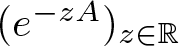 $(e^{-zA})_{z\in {\mathbb{R}}}$ and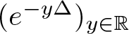 $(e^{-y\Delta })_{y\in {\mathbb{R}}}$. By Plancherel’s formula, we have
 \begin{align}
\int_0^\infty \vert Ce^{-sA}f\vert^2 ds&\leq \int_{-\infty}^\infty \Bigl\vert \int_{-\infty}^\infty c(\nu )f(\nu )e^{is\nu}{\frac{d\nu}{2\pi}} \Bigr\vert^2 ds\nonumber\\
&=\int_{-\infty}^\infty \vert c(\nu )\vert^2\vert f(\nu )\vert^2 d\nu\nonumber\\
&\leq \Vert c\Vert_{L^\infty}^2\Vert f\Vert^2_{L^2}
\end{align}
\begin{align}
\int_0^\infty \vert Ce^{-sA}f\vert^2 ds&\leq \int_{-\infty}^\infty \Bigl\vert \int_{-\infty}^\infty c(\nu )f(\nu )e^{is\nu}{\frac{d\nu}{2\pi}} \Bigr\vert^2 ds\nonumber\\
&=\int_{-\infty}^\infty \vert c(\nu )\vert^2\vert f(\nu )\vert^2 d\nu\nonumber\\
&\leq \Vert c\Vert_{L^\infty}^2\Vert f\Vert^2_{L^2}
\end{align}and likewise
 \begin{align}
\int_0^\infty \vert B^\dagger e^{-sA^\dagger }f\vert^2 ds&\leq \int_{-\infty}^\infty \Bigl\vert \int_{-\infty}^\infty \bar b(\nu )f(\nu )e^{-is\nu}ds\Bigr\vert^2 d\nu\nonumber\\
&=\int_{-\infty}^\infty \vert \bar b(\nu )\vert^2\vert f(\nu )\vert^2 d\nu\nonumber\\
&\leq \Vert b\Vert_{L^\infty}^2\Vert f\Vert^2_{L^2}
\end{align}
\begin{align}
\int_0^\infty \vert B^\dagger e^{-sA^\dagger }f\vert^2 ds&\leq \int_{-\infty}^\infty \Bigl\vert \int_{-\infty}^\infty \bar b(\nu )f(\nu )e^{-is\nu}ds\Bigr\vert^2 d\nu\nonumber\\
&=\int_{-\infty}^\infty \vert \bar b(\nu )\vert^2\vert f(\nu )\vert^2 d\nu\nonumber\\
&\leq \Vert b\Vert_{L^\infty}^2\Vert f\Vert^2_{L^2}
\end{align}so the integrals
 \begin{equation} \int_0^\infty e^{-sA^\dagger}C^\dagger Ce^{-sA}\, ds, \quad \int_0^\infty e^{-sA}BB^\dagger e^{-sA^\dagger}\, ds\end{equation}
are convergent in the weak operator topology and define elements of 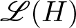 $\mathscr{L}(H)$. Hence, $R_x=\int_x^\infty e^{-sA}BCe^{-sA}\, ds$ is also convergent in the weak operator topology. For $f,h\in \mathscr{D}(A)$, the function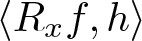 $\langle R_xf,h\rangle$ is differentiable with derivative $\langle (-AR_x-R_xA)f,h\rangle$, so Lyapunov’s equation holds. (In [Reference Megretski, Peller and Treil49], Lyapunov’s equation is also interpreted weakly.)
(ii) As an integral operator on  $L^2((0, \infty ); \mathbb{C})$ the operator $R_x$ has kernel
 \begin{equation}{\frac{c(\kappa )b(k)e^{ix(k+\kappa )}}{2\pi i(k+\kappa )}}\qquad (k, \kappa \gt 0),\end{equation}
which is square integrable.
(iii) Then the impulse response function is
 \begin{equation} \phi (z,y)=Ce^{-zA}e^{-y\Delta}B=\int_{-\infty}^\infty b(v)c(v) e^{ivz+iv^3y}\, {\frac{dv}{2\pi}}\qquad (y,z \gt 0).\end{equation}
Example 9.2. Alternatively, one can assume  $b,c\in C^1_b({\mathbb{R}}; \mathbb{C}),$ and interpret via integration by parts
 \begin{equation}\phi (z,y)=i\int_{-\infty}^\infty {\frac{(b(v)c(v))'}{z+3v^2y}} e^{ivz+iv^3y}\, {\frac{dv}{2\pi}}-i\int_{-\infty}^\infty {\frac{6vy b(v)c(v)}{(z+3v^2y)^2}} e^{ivz+iv^3y}{\frac{dv}{2\pi}},\end{equation}
where these integral are absolutely convergent. In particular, one can choose  $b=c=1$ and obtain the oscillatory integral
 \begin{equation}\phi (z,y)=\int_{-\infty}^\infty e^{ivz+iv^3y}{\frac{dv}{2\pi}}={\frac{1}{(3y)^{1/3}}}{\hbox{Ai}}\Bigl( {\frac{z}{(3y)^{1/3}}}\Bigr)\end{equation}
which is a scaled form of Airy’s function.
Remark 9.3. (i) There is an existence theorem for solutions which are periodic in the spatial variables, so  $(z,y)\in {\mathbb{R}}^2/2\pi{\mathbb{Z}}^2$, where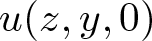 $u(z,y,0)$ is specified as initial data for a Cauchy problem in $t$; see [Reference Bourgain18], [Reference Deconinck and Segur24], [Reference Hadac37].
(ii) Using  $R_x$ from (9.6), one can readily prove the identities of [Reference Ercolani and McKean30, article 5.7] for Fredholm determinant expansions. Whereas Ercolani and McKean show that the tau function satisfies identities consistent with classical theta functions; in Section 10, we use Fredholm determinants in numerical simulations.
(iii) For the Clenshaw–Curtis numerical quadrature in Section 10, it is more convenient to restrict 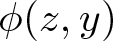 $\phi (z,y)$ to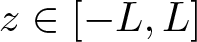 $z\in [-L, L]$ for some large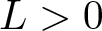 $L \gt 0$, and to use the expansion of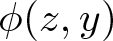 $\phi (z,y)$ in Chebyshev polynomials for $z/L\in [-1,1]$. Equivalently, one considers the Fourier cosine expansion of $\phi (L\cos\theta ,y)$ in the $\theta$ variable. Recall that the Chebyshev polynomials of the first kind are characterized by $T_n(\cos\theta )=\cos (n\theta )$ for $n=1,2, \dots $. From the standard expansion [Reference Whittaker and Watson69, 17.23]
 \begin{equation*} e^{iz\sin t}=J_0(z)+2\sum_{n=1}^\infty \bigl( J_{2n}(z) \cos 2nt +iJ_{2n-1}(z)\sin (2n-1)t\bigr),\end{equation*}
with  $\theta =\pi /2-t$ and $z=L\cos\theta$, we obtain a Fourier cosine expansion
 \begin{align}
\phi (L\cos\theta ,y)&=\int_{-\infty}^\infty b(\nu )c(\nu )e^{i\nu^3y}J_0(L\nu ){\frac{d\nu }{2\pi}}\nonumber\\
&\quad +2\sum_{n=1}^\infty (-1)^n \int_{-\infty}^\infty b(\nu )c(\nu )e^{i\nu^3y}J_{2n}(L\nu ){\frac{d\nu }{2\pi}}\cos 2n\theta \nonumber\\
&\quad -2i
\sum_{n=1}^\infty (-1)^n \int_{-\infty}^\infty b(\nu )c(\nu )e^{i\nu^3y}J_{2n-1}(L\nu ){\frac{d\nu }{2\pi}}\cos (2n-1)\theta ,
\end{align}
\begin{align}
\phi (L\cos\theta ,y)&=\int_{-\infty}^\infty b(\nu )c(\nu )e^{i\nu^3y}J_0(L\nu ){\frac{d\nu }{2\pi}}\nonumber\\
&\quad +2\sum_{n=1}^\infty (-1)^n \int_{-\infty}^\infty b(\nu )c(\nu )e^{i\nu^3y}J_{2n}(L\nu ){\frac{d\nu }{2\pi}}\cos 2n\theta \nonumber\\
&\quad -2i
\sum_{n=1}^\infty (-1)^n \int_{-\infty}^\infty b(\nu )c(\nu )e^{i\nu^3y}J_{2n-1}(L\nu ){\frac{d\nu }{2\pi}}\cos (2n-1)\theta ,
\end{align}where the coefficients involve Bessel functions with integer indices as in (6.18).
10. Numerical simulations
We present numerical simulations of solutions to the KP equation. We use four different numerical approaches as follows:
(1) GLM solution using Riemann Rule approximation (GLM-RR): We solve the linear integral GLM equation, with the coefficients given by semi-additive scattering data representing solutions to the linearized  $KP$ equation. The solution to the linearized equations (10.2) can be analytically advanced to any time $t \gt 0$ and substituted into the GLM equation, which is then solved. For this method we use the left-hand Riemann Rule to approximate the integral in the GLM equation, which is then solved as a large linear system of equations at that time $t \gt 0$;
(2) GLM solution using Clenshaw–Curtis quadrature (GLM-CC): This is similar to the last method except that we use Clenshaw–Curtis quadrature to approximate the integral in the GLM equation. Clenshaw–Curtis quadrature is based on Chebyshev polynomial approximation and its use here is inspired by the approximation method for computing Fredholm determinants developed by Bornemann [Reference Bornemann15], as we outline next;
(3) Fredholm determinant using Nyström–Clenshaw–Curtis method (Det-CC): The solution to the  $KP$ equation is given in terms of the second derivative, with respect to $x$, of the logarithm of the $\tau$-function, which can be expressed as the Fredholm determinant of the scattering data. We use the Nyström–Clenshaw–Curtis method developed by Bornemann [Reference Bornemann15] to approximate Fredholm determinants to very high accuracy;
(4) Direct pseudo-spectral time-stepping approximation (FFT2-exp): This is a direct, exponential split-step, pseudo-spectral method that utilizes the fast Fourier transform (FFT) in both the  $x$- and the $y$- directions. It also utilizes the window method outlined by Kao and Kodama [Reference Kao and Kodama40], to deal with non-periodic boundary conditions. This method is outlined in detail in Blower and Malham [Reference Blower and Malham11, App. B].
We provide further details of these numerical approaches presently. Before doing so, let us outline the direct linearization approach we have outlined in Sections 6–8, and connect that to the direct linearization approach given in Blower and Malham [Reference Blower and Malham11], as well as the expression for the solution via the  $\tau$-function. The $KP$ equation for the field $g=g(x,y;t)$ in potential form is given by
 \begin{equation}
g_t=g_{xxx}+6g_x^2+3{\partial}_x^{-1}g_{yy}.
\end{equation}
\begin{equation}
g_t=g_{xxx}+6g_x^2+3{\partial}_x^{-1}g_{yy}.
\end{equation} This corresponds to the KP equation (1.1) in the case 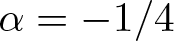 $\alpha=-1/4$,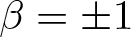 $\beta=\pm1$ and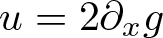 $u=2{\partial}_xg$. The linearized form of the $KP$ equation for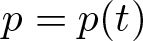 $p=p(t)$ is given by
 \begin{equation}
p_t=p_{xxx}+3{\partial}_x^{-1}p_{yy}.
\end{equation}
\begin{equation}
p_t=p_{xxx}+3{\partial}_x^{-1}p_{yy}.
\end{equation}The linear integral GLM equation is of the form,
 \begin{equation}
P=G({\mathrm{id}}-P),
\end{equation}
\begin{equation}
P=G({\mathrm{id}}-P),
\end{equation}for the solution operator  $G$, or equivalently its kernel, $g$. Here, $P$ is the scattering operator associated with the kernel function solution $p$ solving (10.2). We assume that $P$ is a Hilbert–Schmidt valued integral operator on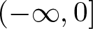 $(-\infty,0]$ with kernel of the form,
 \begin{equation}
p=p(z+x,\zeta+x;y,t).
\end{equation}
\begin{equation}
p=p(z+x,\zeta+x;y,t).
\end{equation} This is the semi-additive form first introduced by Pöppe [Reference Pöppe60] with  $z,\zeta\in(-\infty,0]$ the primary variables parametrizing the operator $P$, while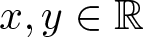 $x,y\in\mathbb R$ and $t\geqslant0$ are regarded as additional parameters. This form guarantees that the first of the following two constraints on $p$ is automatically satisfied:
 \begin{equation}
p_x=p_z+p_{\zeta},
\end{equation}
\begin{equation}
p_x=p_z+p_{\zeta},
\end{equation} \begin{equation}
p_y=p_{zz}-p_{\zeta\zeta}.
\end{equation}
\begin{equation}
p_y=p_{zz}-p_{\zeta\zeta}.
\end{equation} $KP$ hierarchy; see for example [Reference Blower and Malham12]. While our semi-additive assumption for $p$ means that (10.5a) is satisfied, we henceforth assume that $p$ satisfies (10.5b) as well. Using the constraints (10.5), the linearized $KP$ equation (10.2), has the alternative formulation,
 \begin{equation}
p_t=4\,\bigl(p_{zzz}-p_{\zeta\zeta\zeta}\bigr).
\end{equation}
\begin{equation}
p_t=4\,\bigl(p_{zzz}-p_{\zeta\zeta\zeta}\bigr).
\end{equation} Note that if  $P$ is Hilbert–Schmidt valued on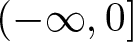 $(-\infty,0]$, then the solution operator $G$ to the GLM equation (10.3) is Hilbert–Schmidt valued on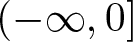 $(-\infty,0]$ as well—see Blower and Malham [Reference Blower and Malham11, Lemma 7]—and the kernel $g=g(z,\zeta;x,y,t)$ of $G$ is square-integrable. Furthermore, $g$ automatically adopts any regularity that $p$ possesses. The solution $g=g(z,\zeta;x,y,t)$ to the GLM equation evaluated at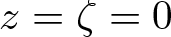 $z=\zeta=0$, i.e. $g=g(0,0;x,y,t)$, satisfies the $KP$ equation (10.1). See, for example, [Reference Blower and Malham11]. Solutions to the $KP$ equation (10.1) can thus be generated by solving the linearized $KP$ equation (10.2), or equivalently here (10.6), and the following linear integral equation for $g=g(0,\zeta;x,y,t)$,
 \begin{equation}
p(x,\zeta+x;y,t)=g(0,\zeta;x,y,t)-\int_{-\infty}^0g(0,\xi;x,y,t)p(\xi+x,\zeta+x;y,t)\,{\mathrm{d}}\xi.
\end{equation}
\begin{equation}
p(x,\zeta+x;y,t)=g(0,\zeta;x,y,t)-\int_{-\infty}^0g(0,\xi;x,y,t)p(\xi+x,\zeta+x;y,t)\,{\mathrm{d}}\xi.
\end{equation} Furthermore, we also know that  $g=g(0,0;x,y,t)$ is given by the trace formula,
 \begin{equation}
g(0,0;x,y,t)=\mathrm{trace}\,\bigl(({\partial}_{\mathfrak{l}}P)V+V({\partial}_{\mathfrak{r}}P)\bigr),
\end{equation}
\begin{equation}
g(0,0;x,y,t)=\mathrm{trace}\,\bigl(({\partial}_{\mathfrak{l}}P)V+V({\partial}_{\mathfrak{r}}P)\bigr),
\end{equation}where  $V:=({\mathrm{id}}-P)^{-1}$; see [Reference Blower and Malham11, Cor. 12]. Here, ${\partial}_{\mathfrak{l}}G$ and ${\partial}_{\mathfrak{r}}G$ represent the trace-class operators with the respective kernels ${\partial}_zg$ and ${\partial}_\zeta g$. In other words we have, $g(0,0;x,y,t)=\mathrm{trace}\,\bigl(({\partial}_x P)V\bigr)$ since ${\partial}_xP={\partial}_{\mathfrak{l}}P+{\partial}_{\mathfrak{r}}P$ using (10.5a). By a standard calculation, we thus have,
 \begin{equation}
g(0,0;x,y,t)=-{\partial}_x\log\mathrm{det}({\mathrm{id}}-P).
\end{equation}
\begin{equation}
g(0,0;x,y,t)=-{\partial}_x\log\mathrm{det}({\mathrm{id}}-P).
\end{equation} The quantity  $\tau:=\mathrm{det}({\mathrm{id}}-P)$ is known as the $\tau$-function, as in Definition 2.7(ii). Thus, in our numerical methods GLM-RR and GLM-CC outlined above, we solve the linear integral equation (10.7), respectively, using the left-hand Riemann Rule and Clenshaw–Curtis quadrature for the integral on the right-hand side. Utilizing either of these quadrature approximations generates a linear algebraic system of equations for the solution $g$ at the nodal points $\zeta_n$. We give more details on this procedure presently. Furthermore, for our numerical method Det-CC, we use the Nyström–Clenshaw–Curtis method developed by Bornemann [Reference Bornemann15] to approximate the $\tau$-function Fredholm determinant. Lastly, in this context, since $g$ solves the potential form of the $KP$ equation (10.1), the solution to the $KP$ equation itself is ${\partial}_xg(0,0;x,y,t)$.
Example 10.1. (One-soliton solution)
Suppose  $a$ and $b$ are real constants and $\Lambda:= a^2-b^2$ and $\Omega:= 4(a^3+b^3)$. Furthermore, suppose $p=p(z+x,\zeta+x;y,t)$ has the form,
 \begin{equation}
p=-(a+b)\exp\bigl(a(z+x)+b(\zeta+x)+\Lambda y+\Omega t\bigr).
\end{equation}
\begin{equation}
p=-(a+b)\exp\bigl(a(z+x)+b(\zeta+x)+\Lambda y+\Omega t\bigr).
\end{equation} Then the solution to the GLM equation (10.7),  $g=g(0,\zeta;x,y,t)$, generates the following one-soliton solution to the $KP$ equation,
 \begin{equation}
{\partial}_xg(0,0;x,y,t)=\tfrac14(a+b)^2\mathrm{sech}^2\Theta,
\end{equation}
\begin{equation}
{\partial}_xg(0,0;x,y,t)=\tfrac14(a+b)^2\mathrm{sech}^2\Theta,
\end{equation}where  $\Theta:=\frac12\bigl((a+b)x+\Lambda y+\Omega t\bigr)$.
Before we discuss the implementation of our numerical methods, let us relate the quantities above to those in Sections 6–8. Suppose the operator  $R=R(x,y,t)$, see for example (1.3) or (7.5), has the form,
 \begin{equation}
R(x,y,t):=\int_0^{\infty}\mathrm{e}^{-b(\xi+x)}\hat{B}(y)C(t)\mathrm{e}^{-a(\xi+x)}\,{\mathrm{d}}\xi.
\end{equation}
\begin{equation}
R(x,y,t):=\int_0^{\infty}\mathrm{e}^{-b(\xi+x)}\hat{B}(y)C(t)\mathrm{e}^{-a(\xi+x)}\,{\mathrm{d}}\xi.
\end{equation} Here, we have assumed that, the operator  $A$ simply represents real multiplication by the constant $a$, and the operator $B=B(y,\zeta)$ has the form,
 \begin{equation}
B(y,\zeta)=\mathrm{e}^{-b\zeta}\hat{B}(y),
\end{equation}
\begin{equation}
B(y,\zeta)=\mathrm{e}^{-b\zeta}\hat{B}(y),
\end{equation}where  $b$ is a real constant. Furthermore, suppose we define the operator from $\mathbb C$ to itself, or function, $\hat{K}=\hat{K}(z,\zeta;x,y,t)$ by,
 \begin{equation}
\hat{K}(z,\zeta;x,y,t):= -C(t)\mathrm{e}^{-a(z+x)}\bigl({\mathrm{id}}+R(x,y,t)\bigr)^{-1}\mathrm{e}^{-b(\zeta+x)}\hat{B}(y).
\end{equation}
\begin{equation}
\hat{K}(z,\zeta;x,y,t):= -C(t)\mathrm{e}^{-a(z+x)}\bigl({\mathrm{id}}+R(x,y,t)\bigr)^{-1}\mathrm{e}^{-b(\zeta+x)}\hat{B}(y).
\end{equation} It is then straightforward to verify that  $\hat{p}(z+x,\zeta+x;y,t):= C(t)\mathrm{e}^{-a(z+x)-b(\zeta+x)}\hat{B}(y)$ and $\hat{K}=\hat{K}(z,\zeta;x,y,t)$ satisfy the linear integral equation,
 \begin{equation}
\hat{p}(z+x,\zeta+x;y,t)+\hat{K}(z,\zeta;x,y,t)+\int_0^\infty K(z,\xi;x,y,t)\,\hat{p}(\xi+x,\zeta+x;y,t)\,{\mathrm{d}}\xi=0.
\end{equation}
\begin{equation}
\hat{p}(z+x,\zeta+x;y,t)+\hat{K}(z,\zeta;x,y,t)+\int_0^\infty K(z,\xi;x,y,t)\,\hat{p}(\xi+x,\zeta+x;y,t)\,{\mathrm{d}}\xi=0.
\end{equation}If we make the change of variables,
 \begin{equation}
\xi\to-\xi,\qquad z\to-z,\qquad \zeta\to-\zeta,\qquad x\to-x,
\end{equation}
\begin{equation}
\xi\to-\xi,\qquad z\to-z,\qquad \zeta\to-\zeta,\qquad x\to-x,
\end{equation}and set,
 \begin{equation}
p(z+x,\zeta+x;y,t):=-\hat{p}(-z-x,-\zeta-x;y,t)
\end{equation}
\begin{equation}
p(z+x,\zeta+x;y,t):=-\hat{p}(-z-x,-\zeta-x;y,t)
\end{equation}and
 \begin{equation}
g(z,\zeta;x,y,t):=\hat{K}(-z,-\zeta;-x,y,t),
\end{equation}
\begin{equation}
g(z,\zeta;x,y,t):=\hat{K}(-z,-\zeta;-x,y,t),
\end{equation} $p$ and $g$ satisfy the GLM equation $P=G({\mathrm{id}}-P)$, i.e.
 \begin{equation}
p(z+x,\zeta+x;y,t)=g(z,\zeta;x,y,t)-\int_{-\infty}^0g(z,\xi;x,y,t)p(\xi+x,\zeta+x;y,t){\mathrm{d}}\xi.
\end{equation}
\begin{equation}
p(z+x,\zeta+x;y,t)=g(z,\zeta;x,y,t)-\int_{-\infty}^0g(z,\xi;x,y,t)p(\xi+x,\zeta+x;y,t){\mathrm{d}}\xi.
\end{equation} This generates (10.7) when we set  $z=0$.
Example 10.2. (One-soliton solution: reprise)
Recall the one-soliton solution we outlined in Example 10.1, and in particular the quantities  $\Lambda$ and $\Omega$. In the context of the operator $R$ and kernels $\hat{p}$ and $\hat{K}$, suppose the kernel of the operator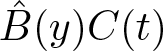 $\hat{B}(y)C(t)$ has the separable form,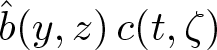 $\hat{b}(y,z)\,c(t,\zeta)$, where $z$ and $\zeta$ are the primary variables. Further suppose that $\hat{b}$ and $c$ have the respective specific forms,
 \begin{equation*}
\hat{b}(y,z)=B_0\mathrm{e}^{-az+\Lambda y}\qquad\text{and}\qquad c(t,\zeta)=C_0\mathrm{e}^{-b\zeta+\Omega t},
\end{equation*}
\begin{equation*}
\hat{b}(y,z)=B_0\mathrm{e}^{-az+\Lambda y}\qquad\text{and}\qquad c(t,\zeta)=C_0\mathrm{e}^{-b\zeta+\Omega t},
\end{equation*}where the constants  $B_0$ and $C_0$ satisfy $B_0C_0=(a+b)^2$. Then the kernel $r=r(z,\zeta;x,y,t)$ of the operator $R=R(x,y,t)$ has the form,
 \begin{equation*}
r(z,\zeta;x,y,t)=(a+b)\mathrm{e}^{-a(z+x)-b(\zeta+x)+\Lambda y+\Omega t}.
\end{equation*}
\begin{equation*}
r(z,\zeta;x,y,t)=(a+b)\mathrm{e}^{-a(z+x)-b(\zeta+x)+\Lambda y+\Omega t}.
\end{equation*} This kernel form matches the one-soliton semi-additive form for  $p$ in (10.10)—taking into account the transformation (10.16a).
Let us now outline in detail the four numerical algorithms we used to compute solutions to the  $KP$ equation. For all four numerical methods, we truncate the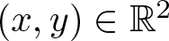 $(x,y)\in\mathbb R^2$ domain to $[-L_x/2,L_x/2]\times[-L_y/2,L_y/2]$ for sufficiently large domain lengths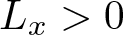 $L_x \gt 0$ and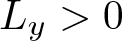 $L_y \gt 0$. First, we outline the simple solution method, GLM-RR, that solves the linear integral GLM equation, by using the left-hand Riemann Rule to approximate the integral therein. Our goal is to compute $g=g(0,0;x,y,t)$. To achieve this, for given scattering data $p$, and given $x\in[-L_x/2,L_x/2]$, $y\in[-L_y/2,L_y/2]$ and $t\geqslant0$, we numerically solve the GLM equation (10.7) for $g=g(0,\zeta;x,y,t)$ and then set $\zeta=0$. In practice we use $N_x$ nodal points $x_n$ in the truncated $x$-domain and $N_y$ nodal points $y_{n^\prime}$ in the truncated $y$-domain. For each nodal point-pair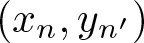 $(x_n,y_{n^\prime})$ and any given fixed $t\geqslant0$, we numerically solve (10.7) as follows. Note that $\zeta,\xi\in[-L_x/2,0]$. We use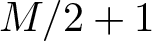 $M/2+1$ nodal points $\zeta_m$ and $\xi_{m^\prime}$ for these variables in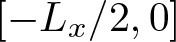 $[-L_x/2,0]$, with separation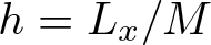 $h=L_x/M$. We always take $M$ to be even. Using each of the nodal point $\zeta_m$, we generate the row vector $\widehat{P}$ of length ‘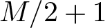 $M/2+1$’ containing the values $p(x_n,\zeta_m+x_n;y_{n^\prime},t)$ for $m\in\{0,1,\ldots,M/2\}$. Note that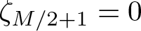 $\zeta_{M/2+1}=0$. Furthermore, for each of the nodal point pairs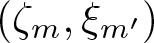 $(\zeta_m,\xi_{m^\prime})$, we generate the matrix $\widehat{Q}$ of size $(M/2+1)\times(M/2+1)$ containing the values $p(\xi_{m^\prime}+x_n,\zeta_m+x_n;y_{n^\prime},t)$ for $m^\prime,m\in(0,1,\ldots,M/2)$. Suppose that $\widehat{G}$ is the row vector of unknown values $g(0,\zeta_m;x_n,y_{n^\prime},t)$ for $m\in(0,1,\ldots,M/2)$. We then solve the linear algebraic system,
 \begin{equation}
\widehat{P}=\widehat{G}(I-h\widehat{Q}),
\end{equation}
\begin{equation}
\widehat{P}=\widehat{G}(I-h\widehat{Q}),
\end{equation}for  $\widehat{G}$, where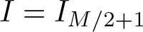 $I=I_{M/2+1}$ is the $(M/2+1)\times(M/2+1)$ identity matrix. The matrix product ‘ $h\widehat{G}\widehat{Q}$’ with the multiplicative scaling $h$, naturally implements the left-hand Riemann Rule. We solve the linear system in (10.18) using Gaussian elimination. For a given $t\geqslant0$, the procedure just outlined, is carried out for each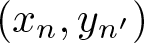 $(x_n,y_{n^\prime})$ with $n\in\{0,1,\ldots,N_x\}$ and $n^\prime\in\{0,1.\ldots,N_y\}$. For each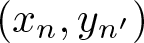 $(x_n,y_{n^\prime})$ we extract the final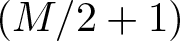 $(M/2+1)$th component of $\widehat{G}$ which represents an approximation for $g(0,0;x_n,y_{n^\prime},t)$. This outlines the GLM-RR method. We compute the solution to the $KP$ equation, namely ${\partial}_xg(0,0;x_n,y_{n^\prime},t)$, by approximating the derivative via a finite difference.
Second, we outline the GLM-CC method, inspired by the method for computing Fredholm determinants developed by Bornemann [Reference Bornemann15]. To begin with, this method follows that of the GLM-RR method, we truncate the 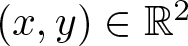 $(x,y)\in\mathbb R^2$ domain in precisely the same way and utilize the nodes $x_n$ and $y_{n^\prime}$ as outlined above. The difference comes into play with the choice of the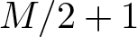 $M/2+1$ nodal points $\zeta_m$ and $\xi_{m^\prime}$ in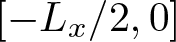 $[-L_x/2,0]$. Here, we choose these nodal points according to the Clenshaw–Curtis quadrature rule approximation for the integral term in (10.7). Indeed, using the notation,
 \begin{equation*}
\rho(\xi,\zeta;x_n,y_{n^\prime},t):= p(\xi+x_n,\zeta+x_n;y_{n^\prime},t)\quad\text{and}\quad \gamma(\zeta;x_n,y_{n^\prime},t):= g(0,\zeta;x_n,y_{n^\prime},t),
\end{equation*}
\begin{equation*}
\rho(\xi,\zeta;x_n,y_{n^\prime},t):= p(\xi+x_n,\zeta+x_n;y_{n^\prime},t)\quad\text{and}\quad \gamma(\zeta;x_n,y_{n^\prime},t):= g(0,\zeta;x_n,y_{n^\prime},t),
\end{equation*}and then suppressing the implicit  $x_n$, $y_{n^\prime}$ and $t$-dependence in $\gamma$ and $\rho$, we approximate,
 \begin{equation}
\int_{-L_x/2}^0\gamma(\xi)\rho(\xi,\zeta_m)\,{\mathrm{d}}\xi\approx\sum_{m^\prime=0}^{M/2+1}w_{m^\prime}\gamma(\xi_{m^\prime})\rho(\xi_{m^\prime},\zeta_m).
\end{equation}
\begin{equation}
\int_{-L_x/2}^0\gamma(\xi)\rho(\xi,\zeta_m)\,{\mathrm{d}}\xi\approx\sum_{m^\prime=0}^{M/2+1}w_{m^\prime}\gamma(\xi_{m^\prime})\rho(\xi_{m^\prime},\zeta_m).
\end{equation} Here,  $\zeta_m$ and $\xi_{m^\prime}$ are chosen to be the Clenshaw–Curtis nodal points and the $w_{m}$ are the Clenshaw–Curtis quadrature weights. Clenshaw–Curtis quadrature is based on the expansion of the integrand using Chebyshev polynomials of the first kind. The nodal points and weights are given explicitly in Bornemann [Reference Bornemann15, p. 909], including a Matlab code for generating them, which in fact, we utilized directly. Bornemann points out that alternatively, Gauss–Legendre quadrature could also be used; however, Clenshaw–Curtis quadrature is more efficient. Thus, for each nodal point pair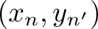 $(x_n,y_{n^\prime})$ and any given fixed $t\geqslant0$, we construct the row vectors $\widehat{P}$ and $\widehat{G}$ and the matrix $\widehat{Q}$, as above, except now based on the Clenshaw–Curtis nodal points $\zeta_m$ and $\xi_{m^\prime}$, which are not uniformly distributed. Let $W$ denote the diagonal matrix of Clenshaw–Curtis quadrature weights. We then solve the linear algebraic system,
 \begin{equation}
\widehat{P}=\widehat{G}(I-W\widehat{Q}),
\end{equation}
\begin{equation}
\widehat{P}=\widehat{G}(I-W\widehat{Q}),
\end{equation}for  $\widehat{G}$, again using Gaussian elimination. The Clenshaw–Curtis quadrature approximation is implicit in the matrix product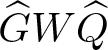 $\widehat{G}W\widehat{Q}$. As above, for a given $t\geqslant0$ and for each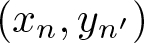 $(x_n,y_{n^\prime})$ with $n\in\{0,1,\ldots,N_x\}$ and $n^\prime\in\{0,1.\ldots,N_y\}$, we solve the linear system (10.20) and extract the final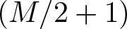 $(M/2+1)$th component of $\widehat{G}$ which represents our approximation for $g(0,0;x_n,y_{n^\prime},t)$. This outlines the GLM-CC method. We again use a finite difference approximation to compute ${\partial}_xg(0,0;x_n,y_{n^\prime},t)$.
Third, we now outline the Det-CC solution method based on the method for computing Fredholm determinants developed by Bornemann [Reference Bornemann15]. Again, initially this follows the set-up of the GLM-CC method, we truncate the 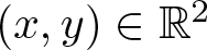 $(x,y)\in\mathbb R^2$ domain as above and utilize the uniformly distributed nodes $x_n$ and $y_{n^\prime}$. Our goal here is to compute the quantity ‘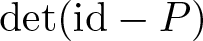 $\mathrm{det}({\mathrm{id}}-P)$’ in the formula (10.9). Bornemann [Reference Bornemann15] provides a simple and accurate approximation formula for computing such a determinant based on Clenshaw–Curtis quadrature. Using the same notation to that outlined above for the GLM-CC method, Bornemann [Reference Bornemann15, p. 890, 894] suggests we compute,
 \begin{equation}
\mathrm{det}({\mathrm{id}}-P)\approx\det\bigl(I-W^{1/2}\widehat{Q}W^{1/2}\bigr),
\end{equation}
\begin{equation}
\mathrm{det}({\mathrm{id}}-P)\approx\det\bigl(I-W^{1/2}\widehat{Q}W^{1/2}\bigr),
\end{equation}where  $W^{1/2}$ is the diagonal matrix of entries consisting of the square roots of the Clenshaw–Curtis weights. We compute this approximation for any given $t\geqslant0$ and for each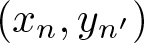 $(x_n,y_{n^\prime})$ with $n\in\{0,1,\ldots,N_x\}$ and $n^\prime\in\{0,1.\ldots,N_y\}$. This outlines the Det-CC method. The approximate solution to the $KP$ equation can be computed by approximating the partial derivative ${\partial}_x^2$ of this determinant approximation using a second-order central difference scheme. A comprehensive error and performance analysis is provided in Bornemann [Reference Bornemann15]. We remark on this in our implementation in Example 10.3 below. Fourth, we now outline the exponential split-step pseudo-spectral algorithm we used to directly integrate the $KP$ equations. For convenience, suppose $A$ denotes the linear $KP$ operator, $A:={\partial}_x^3+3{\partial}_x^{-1}{\partial}_y^2$. Then the exponential split-step we use to integrate the $KP$ equation 10.1 is given by,
 \begin{align*}
v_\ell&=\exp\bigl(\Delta t\,\mathscr{F}(A)\bigr)\,\hat{u}_\ell,\\
\hat{u}_{\ell+1}&=v_\ell-\Delta t\,\mathscr{F}\bigl(\mathrm{N}(v_\ell)\bigr),
\end{align*}
\begin{align*}
v_\ell&=\exp\bigl(\Delta t\,\mathscr{F}(A)\bigr)\,\hat{u}_\ell,\\
\hat{u}_{\ell+1}&=v_\ell-\Delta t\,\mathscr{F}\bigl(\mathrm{N}(v_\ell)\bigr),
\end{align*}where  $\mathrm{N}(v)=6{\partial}_x(\mathscr{F}^{-1}v)^2$. Here, $\mathscr{F}$ represents the two-dimensional Fourier transform, and $\hat{u}_\ell$ is the two-dimensional Fourier transform of the approximate solution $u$ to the $KP$ equation at time $t_\ell\in\{0\}\cup\mathbb N$. The quantity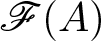 $\mathscr{F}(A)$ represents the Fourier transform of the operator $A$. In practice, if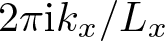 $2\pi\mathrm{i}k_x/L_x$ and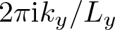 $2\pi\mathrm{i}k_y/L_y$ are the wavenumbers, respectively, in the $x$- and $y$- directions, we set,
 \begin{equation*}
\bigl(\mathscr{F}(A)\bigr)(k_x,k_y)=(2\pi\mathrm{i}k_x/L_x)^3+3\frac{(2\pi\mathrm{i}k_y/L_y)^2}{(2\pi\mathrm{i}k_x/L_x)+2\pi\delta}.
\end{equation*}
\begin{equation*}
\bigl(\mathscr{F}(A)\bigr)(k_x,k_y)=(2\pi\mathrm{i}k_x/L_x)^3+3\frac{(2\pi\mathrm{i}k_y/L_y)^2}{(2\pi\mathrm{i}k_x/L_x)+2\pi\delta}.
\end{equation*} Here, following Klein and Roidot [Reference Klein and Roidot41, p. 3341], we have approximated the Fourier transform of  ${\partial}_x^{-1}$ by $1/(2\pi\mathrm{i}k_x/L_x+2\pi\delta)$, where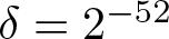 $\delta=2^{-52}$. The initial data is generated by numerically solving the GLM equation, using the GLM-CC method, for the given scattering data $p$ at time $t=0$, as outlined above. We use a pseudo-spectral algorithm due to its simplicity and efficiency, see, for example, Klein and Saut [Reference Klein and Saut42] and Grava, Klein, and Pitton [Reference Grava, Klein and Pitton36]. To deal with the fact that the solutions we compute are not periodic, we use the ‘window method’ employed by Kao and Kodama [Reference Kao and Kodama40]. Precise details on this method can be found in Blower and Malham [Reference Blower and Malham11, App. B]. The FFT2-exp method we have employed thus combines the exponential split-step pseudo-spectral algorithm with the ‘window method’.
Example 10.3. (Two-soliton interaction)
We use the four algorithms we have outlined above to generate the solution to the  $KP$ equation corresponding to the following two-soliton interaction scattering data. Suppose $p_1$ is the one-soliton scattering data of the form (10.10) generated by the values $a=1.55$ and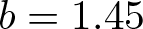 $b=1.45$, while $p_2$ is the one-soliton scattering data (10.10) generated by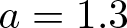 $a=1.3$ and $b=0$. In this example, we assume the two-soliton interaction scattering data, $p=p_1+p_2$. In our computations, we assume the truncated domain lengths to be $L_x=L_y=10\pi$. Figure 1 shows the solution ${\partial}_xg(0,0;x,y,t)$ computed at $t=0$, both using the GLM-CC method and the Det-CC method, corresponding to the two-soliton interaction scattering data $p$ with $t=0$. In both cases the number of Clenshaw–Curtis nodal points used was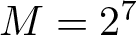 $M=2^7$, while the number of $(x,y)$ evaluation points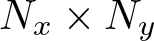 $N_x\times N_y$ was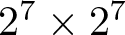 $2^7\times 2^7$. Figure 2 shows the solution ${\partial}_xg(0,0;x,y,t)$ computed at $t=0.25$, using the GLM-CC, Det-CC and FFT2-exp methods. In the case of the GLM-CC and Det-CC methods, the two-soliton interaction scattering data $p$ with $t=0.25$ was used. In both cases, the number of Clenshaw–Curtis nodal points and $(x,y)$ evaluation points used was the same as for the $t=0$ case. In the case of the FFT2-exp method, the number of $(x,y)$ evaluation points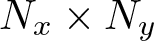 $N_x\times N_y$ used, was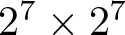 $2^7\times 2^7$, while $10^4$ timesteps where used on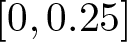 $[0,0.25]$. The initial data used for the FFT2-exp method was the output of the GLM-CC method at $t=0$ shown in the top panel of Figure 1. We observe from Figure 2 that the accuracy of the FFT2-exp method does not match that of the GLM-CC and Det-CC methods. Note that in both Figures 1 and 2, we only display the domain region $(x,y)\in[-L_x/4.L_x/2]\times[-L_y/4,L_y/2]$ and the $x$- and $y$- coordinates of $p$ are shifted so the interaction occurs in this region.
We plot the two-soliton interaction solution outlined in Example 10.3 at  $t=0$. The top panel set shows the solution computed by numerically solving the GLM equation (10.7) using Clenshaw–Curtis quadrature, i.e. the GLM-CC method. The bottom panel set shows the solution computed using the $\tau$-function Fredholm determinant, i.e. using the Nyström–Clenshaw–Curtis method Det-CC. The right-hand panels show the corresponding contour plots.

1 Long description
The image A showing a three-dimensional surface plot titled GLM Clenshaw-Curtis method T=0. The x-axis is labeled x with tick labels minus 5, 0, 5, 10, 15. The y-axis is labeled y with tick labels minus 5, 0, 5, 10, 15. The vertical axis is labeled g subscript x with tick labels 0.5, 0, minus 0.5, minus 1, minus 1.5, minus 2, minus 2.5. No unit text is shown for x, y, or g subscript x. The surface is near 0 over much of the domain, then drops sharply for x values near 10 to 15, reaching values below minus 2. Several repeating trough-like bands appear along the steep drop region. The image B showing a contour plot titled GLM Clenshaw-Curtis method, partial subscript x g: T=0. The x-axis is labeled x with tick labels minus 6, minus 4, minus 2, 0, 2, 4, 6, 8, 10, 12, 14. The y-axis is labeled y with tick labels minus 6, minus 4, minus 2, 0, 2, 4, 6, 8, 10, 12, 14. No unit text is shown for x or y. Contours form a narrow, near-vertical high-gradient band for x values around 11 to 13 across most y values. Additional contours approach the band along diagonal paths from lower x values at higher y values and the contour spacing tightens around x about 11 to 12 and y about 6 to 8. The image C showing a three-dimensional surface plot titled Determinant Nystrom method T=0. The x-axis is labeled x with tick labels minus 5, 0, 5, 10, 15. The y-axis is labeled y with tick labels minus 5, 0, 5, 10, 15. The vertical axis is labeled partial subscript x squared log tau with tick labels 0.5, 0, minus 0.5, minus 1, minus 1.5, minus 2, minus 2.5. No unit text is shown for x, y, or partial subscript x squared log tau. The surface is near 0 over much of the domain and drops sharply for x values near 10 to 15, reaching values below minus 2, with repeating trough-like bands along the steep drop region. The image D showing a contour plot titled Determinant Nystrom method, partial subscript x squared log tau: T=0. The x-axis is labeled x with tick labels minus 6, minus 4, minus 2, 0, 2, 4, 6, 8, 10, 12, 14. The y-axis is labeled y with tick labels minus 6, minus 4, minus 2, 0, 2, 4, 6, 8, 10, 12, 14. No unit text is shown for x or y. Contours form a narrow, near-vertical high-gradient band for x values around 11 to 13 across most y values. Diagonal contour paths approach the band from lower x values at higher y values and contour spacing tightens around x about 11 to 12 and y about 6 to 8.
We plot the two-soliton interaction solution outlined in Example 10.3 at  $t=0.25$. The top panel set shows the solution computed by numerically solving the GLM equation (10.7) using the GLM-CC method. The middle panel set shows the solution computed using the Det-CC method. The bottom panel set shows the solution computed by direct numerical integration using the FFT2-exp method. The right-hand panels show the corresponding contour plots.

Figure 2 Long description
The image A showing a 3D surface plot titled “GLM Clenshaw Curtis method t=0.25”. The horizontal axes are labeled x and y. The vertical axis is labeled partial derivative x g. The x-axis shows tick labels from minus 5 to 15. The y-axis shows tick labels from minus 5 to 15. The partial derivative x g axis shows tick labels from minus 0.5 to 0.5. The surface includes a broad, nearly flat region and a steep ridge like structure that bends across the plot, with a deep trough adjacent to the ridge. The image B showing a contour plot titled “GLM Clenshaw Curtis method, partial derivative x g: T=0.25”. The x-axis is labeled x with tick labels from minus 6 to 14. The y-axis is labeled y with tick labels from minus 6 to 14. Contour lines form a narrow, nearly vertical band centered near x around 9 to 10 and several diagonal contour bands that intersect this vertical band. The image C showing a 3D surface plot titled “Determinant Nystrom method t=0.25”. The horizontal axes are labeled x and y. The vertical axis is labeled partial derivative x g. The x-axis shows tick labels from minus 5 to 15. The y-axis shows tick labels from minus 5 to 15. The partial derivative x g axis shows tick labels from minus 0.5 to 0.5. The surface shows a broad, nearly flat region and a steep ridge like structure with an adjacent trough, similar in placement to image A. The image D showing a contour plot titled “Determinant Nystrom method, partial derivative x g: T=0.25”. The x-axis is labeled x with tick labels from minus 6 to 14. The y-axis is labeled y with tick labels from minus 6 to 14. Contour lines form a narrow, nearly vertical band near x around 9 to 10, with multiple diagonal contour bands crossing it. The image E showing a 3D surface plot titled “Direct pseudo spectral (FFT2) method t=0.25”. The horizontal axes are labeled x and y. The vertical axis is labeled partial derivative x g. The x-axis shows tick labels from minus 5 to 15. The y-axis shows tick labels from minus 5 to 15. The partial derivative x g axis shows tick labels from minus 0.5 to 0.5. The surface appears more rippled, with multiple smaller undulations across the flatter region and a steep ridge and trough structure toward the right side. The image F showing a contour plot titled “Direct pseudo spectral (FFT2) method, partial derivative x g: T=0.25”. The x-axis is labeled x with tick labels from minus 6 to 14. The y-axis is labeled y with tick labels from minus 6 to 14. Contour lines include a narrow, nearly vertical band near x around 9 to 10, intersected by diagonal contour bands, with additional irregular contour loops and waviness compared with images B and D.
11. Exponential convergence
Herein, we compare the performance of the numerical methods we used in Section 10, in particular the GLM-RR, GLM-CC, and Det-CC methods. See Figures 3 and 4. The remarkable properties of the use of Clenshaw–Curtis quadrature to compute Fredholm determinants are comprehensively outlined in Bornemann [Reference Bornemann15] and [Reference Bornemann16]. In the left panels in Figure 3, we estimated the errors involved in computing using the GLM-RR, GLM-CC, and Det-CC methods as follows. We replaced the scattering data  $p=p_1+p_2$ for the two-soliton interaction solution outlined in Example 10.3, by, the perturbed form,
We plot the errors associated with GLM-RR and GLM-CC methods for solving the GLM equation, and Det-CC method for computing the  $\tau$-function Fredholm determinant, associated with the perturbed data (11.1) at $t=0.25$. The top panels show the root-mean-square error (left panel) and the maximum error (right panel) versus the number of nodal points $M$ used in the Clenshaw–Curtis or Riemann Rule quadrature to compute the solutions at each point $(x,y)\in[-L_x/2,L_x/2]\times[-L_y/2,L_y/2]$. The bottom left panel shows the root-mean-square error versus the CPU time required to compute the solution, corresponding to the top left panel plot. The bottom right panel shows the pointwise error (right panel) versus the number of nodal points $M$. A generic point was chosen, in this case $x=y=6.4$, to compute the pointwise error.

Figure 3 Long description
The first graph shows RMS error vs number of nodes at T equals 0.25. The x-axis is labeled M, ranging from 0 to 600 and the y-axis is RMS error, from 10 superscript 2 to 10 superscript negative 5. The GLM: Clenshaw-Curtis method starts high and decreases sharply, leveling off around 200 nodes. Det: Clenshaw-Curtis and GLM: Riemann Rule follow similar trends but with lower initial errors. The second graph displays maximum error vs number of nodes at T equals 0.25. The x-axis is M, from 0 to 600 and the y-axis is max error, from 10 superscript 5 to 10 superscript negative 25. GLM: Clenshaw-Curtis and its modified versions show decreasing errors, with mod2 achieving the lowest. Det: Clenshaw-Curtis and its variants also decrease, but at a slower rate. The third graph presents RMS error vs CPU time at T equals 0.25. The x-axis is CPU time, from 1.29 to 1.39 and the y-axis is RMS error, from 10 superscript 2 to 10 superscript negative 5. GLM: Clenshaw-Curtis shows a rapid decrease in error with increasing CPU time, while Det: Clenshaw-Curtis and GLM: Riemann Rule have similar trends but start with lower errors. The fourth graph illustrates pointwise error vs number of nodes at T equals 0.25. The x-axis is M, from 0 to 600 and the y-axis is pointwise error, from 10 superscript 0 to 10 superscript negative 16. GLM: Clenshaw-Curtis decreases steadily, with Det: Clenshaw-Curtis and GLM: Riemann Rule showing similar patterns but with lower initial errors. Overall, the graphs highlight the effectiveness of different methods in reducing errors as M or CPU time increases, with modified versions showing improved performance in some cases.
The top panel shows the error in the solution to the GLM equation for the perturbed data (11.1) at  $t=0.25$, computed with the Det-CC method using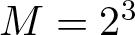 $M=2^3$, i.e. the difference between the solution computed using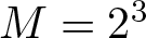 $M=2^3$ Clenshaw–Curtis nodal points and the solution computed using the maximum number of such nodal points that we used, namely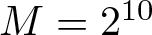 $M=2^{10}$. The middle panel shows the same plot but for the case of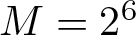 $M=2^6$ versus the maximum number of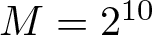 $M=2^{10}$ nodal points. The bottom panel shows the estimate (11.2) for the number of digits of accuracy lost in the Det-CC method.

Figure 4 Long description
Three 3D surface plots are arranged vertically, each examining numerical performance of the Det-CC method applied to the GLM equation with perturbed data at time t equals 0.25. The image A showing the error surface for the configuration where M equals 2 superscript 3 nodal points versus the maximum of M equals 2 superscript 10 nodal points. The x-axis is labeled with the spatial variable, ranging from approximately minus 10 to 10. The y-axis is labeled with the second spatial variable, ranging from approximately minus 10 to 10. The z-axis represents the difference between the solution computed using M equals 2 superscript 3 Clenshaw-Curtis nodal points and the solution computed using M equals 2 superscript 10 Clenshaw-Curtis nodal points. The surface is largely flat across most of the domain, with a sharply concentrated peak region visible near the center-right portion of the surface. The peak rises steeply from the otherwise near-zero base level, indicating that the error is localized rather than distributed uniformly. The image B showing the error surface for the configuration where M equals 2 superscript 6 nodal points versus the maximum of M equals 2 superscript 10 nodal points. The x-axis and y-axis span the same spatial ranges as the first surface. The z-axis again represents the difference between solutions at M equals 2 superscript 6 and M equals 2 superscript 10 Clenshaw-Curtis nodal points. The surface is flatter overall compared to the first surface, with a smaller and less prominent peak visible in the same spatial region. This indicates a reduction in error magnitude when more nodal points are used. The image C showing the estimated number of digits of accuracy lost in the Det-CC method. The x-axis and y-axis span the same spatial domain as the previous two surfaces. The z-axis represents the estimated digits of accuracy lost. The surface shows a smooth gradient across the domain, with elevated values concentrated in one region, indicating where the greatest loss of numerical accuracy occurs relative to the rest of the computational domain.
 \begin{equation}
p\,\bigl(1+\exp(-\Theta_1^2)/10^2\bigr)\,\bigl(1+\exp(-\Theta_2^2)\bigr).
\end{equation}
\begin{equation}
p\,\bigl(1+\exp(-\Theta_1^2)/10^2\bigr)\,\bigl(1+\exp(-\Theta_2^2)\bigr).
\end{equation} Here,  $\Theta_i:=\frac12\bigl(a_i(z+x)+b_i(\zeta+x)+\Lambda_iy+\Omega_it\bigr)$ for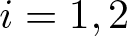 $i=1,2$, with the coefficients $a_1$, $a_2$, $b_1$ and $b_2$ those corresponding to $p_1$ and $p_2$, respectively, as outlined in Example 10.3 with the $\Lambda_i$ and $\Omega_i$ defined accordingly. Note that this perturbed form for $p$ does not generate a solution to the KP equation. However, our goal herein is to demonstrate the exponential convergence of the GLM-CC and Det-CC methods. Hence, we have chosen a form for $p$ that is analytic, but not the two-soliton solution for which the $\tau$-function collapses to a finite determinant. We computed the corresponding GLM solution and Fredholm determinant at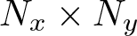 $N_x\times N_y$ evaluation points with $N_x=N_y=2^6$. In each case we used $2^m$ quadrature nodal points as $m$ varied from $2$ through to $10$. In the case of the GLM-CC computations, we evaluated the numerical error by considering the difference of the solution $g(0,0;x_n,y_{n^\prime},t)$ computed using $2^2$, $2^3$, $\ldots$, $2^9$ Clenshaw–Curtis nodal points, to the corresponding solution $g(0,0;x_n,y_{n^\prime},t)$ computed using $2^{10}$ Clenshaw–Curtis nodal points. For the GLM-RR method, instead of Clenshaw–Curtis quadrature nodal points, we just use the corresponding number of uniform quadrature nodal points. In the case of the Det-CC method, we computed the difference between $\tau:=\mathrm{det}({\mathrm{id}}-P)$ in (10.21), i.e.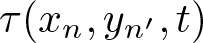 $\tau(x_n,y_{n^\prime},t)$ computed using $2^2$, $2^3$, $\ldots$, $2^9$ Clenshaw–Curtis nodal points, and the corresponding $\tau$ function computed using $2^{10}$ Clenshaw–Curtis nodal points. For all methods, the time was set to be $t=0.25$. We estimated the root-mean-square (RMS) error in the left two panels in Figure 3 by computing the Frobenius norm scaled by $(L_xL_y/N_xN_y)^{1/2}$, of all the differences across the evaluation points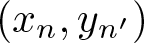 $(x_n,y_{n^\prime})$ for all $n\in\{0,1,\ldots,N_x\}$ and $n^\prime\in\{0,1,\ldots,N_y\}$.
The top left panel in Figure 3 shows a log-linear plot of the RMS error versus the number of Clenshaw–Curtis nodal points  $M$, while the lower left panel shows a log-linear plot of the RMS error versus the CPU time required to compute the solution for the corresponding number of Clenshaw–Curtis nodal points. The superior error of the GLM-CC and Det-CC methods compared to the GLM-RR method is immediately apparent, though their computation times are only slightly better. Indeed, as Bornemann [Reference Bornemann15, p. 891] points out, for analytic kernels, we expect exponential convergence for the Det-CC method, and the form (11.1) for the scattering data we have assumed here is analytic. In the bottom right panel in Figure 3, in a log-linear plot, we show the convergence of the GLM-RR, GLM-CC, and Det-CC methods at a specific generic point, in this case $x=y=6.4$. We observe that the convergence of both the Det-CC and GLM-CC methods is exponential, and indeed, it hits an error of order $10^{-15}$ relatively rapidly.
This exponential convergence can also be seen in the top panels in Figure 3, though the convergence flattens off at roughly  $10^{-5}$ for $M$ beyond $2^5$. This can be explained as follows. In the top panel in Figure 4, for the perturbed scattering data (11.1) at $t=0.25$ computed with the Det-CC method, we plot the difference between the solution computed using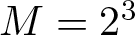 $M=2^3$ Clenshaw–Curtis nodal points and the reference ‘exact’ solution we computed using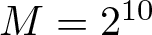 $M=2^{10}$ such nodal points. We observe that this error estimate is smooth everywhere except for the region where $x$ and $y$ are large, close to their maximum values of $5\pi$. We observe some ‘wrinkles’ in this error plot, and the maximum error is of order $10^{-1}$ in this region. The middle panel in Figure 4 shows the same plot but using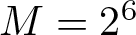 $M=2^6$ nodal points. We observe errors of order $10^{-5}$ in this case, with these errors again larger where $x$ and $y$ are large. All Clenshaw–Curtis nodal points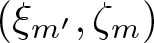 $(\xi_{m^\prime},\zeta_m)$, which are based on Chebyshev nodal points, are interior to the boundary of the domain $[-L_x/2.L_x/2]\times[-L_y/2,L_y/2]$. When $M=2^m$ is small, say with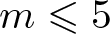 $m\leqslant5$, the largest Clenshaw–Curtis nodal points are still relatively far from the boundary. However, when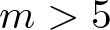 $m \gt 5$, they do become close. Our perturbed scattering data kernel (11.1) grows exponentially for large and positive values of $\xi$, $\zeta$, $x$, and $y$. Indeed, when these values are close to the boundary, $5\pi$, then (11.1) is of order $10^{27}$. The accuracy of the linear algebra computations that underlie the GLM-CC and Det-CC methods is compromised in this situation and delivers the accuracies, of order $10^{-1}$ when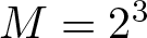 $M=2^3$ and order $10^{-5}$ when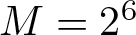 $M=2^6$, observed in Figure 4. We also observe this in the top right panel in Figure 3. Therein, for the GLM-CC and Det-CC methods, we observe the exponential convergence of the maximum norm of the error for small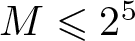 $M\leqslant2^5$, but once $M$ is larger than this, the maximum norm of the error over the whole domain reverts to an error of order $10^{-5}$. In the top right panel in Figure 3, we also computed the maximum norm of the error for the GLM-CC and Det-CC methods over the restricted domains for which $x\in[-5\pi,10.8]$, indicated by the ‘mod’ label, and for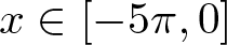 $x\in[-5\pi,0]$, indicated by the ‘mod2’ label. In the first case, we observe that the maximum norm errors flatten out at about $10^{-7}$, while in the second case, they flatten out at roughly $10^{-13}$. This indicates that the influence of accuracy loss due to very large values of $p$ in our computations naturally recedes as $x_n$ decreases. And this is consistent with our pointwise error estimate in the bottom right panel in Figure 3, for which $x=y=6.4$. Since the RMS error estimate is global, this also explains why this error estimate in the two left panels in Figure 3 flattens out at roughly $10^{-5}$. We observe analogous results when, instead of the perturbed scattering data (11.1), we use the two-soliton interaction data $p=p_1+p_2$ in Example 10.3.
Remark 11.1. (Other sources of accuracy loss)
Bornemann [Reference Bornemann15, p. 884] outlines that if  $\det({\mathrm{id}}-P)\ll\|P\|_{\mathscr{L}^2}$, where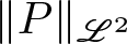 $\|P\|_{\mathscr{L}^2}$ is the Hilbert–Schmidt norm of $P$, then a ‘conservative estimate’ predicts a loss of some digits of accuracy, when computing the Fredholm determinant using Nyström–Clenshaw–Curtis quadrature, of at most,
 \begin{equation}
\log_{10}\biggl(\frac{\sqrt{M}\cdot\|P\|_{\mathscr{L}^2}}{\det({\mathrm{id}}-P)}\biggr),
\end{equation}
\begin{equation}
\log_{10}\biggl(\frac{\sqrt{M}\cdot\|P\|_{\mathscr{L}^2}}{\det({\mathrm{id}}-P)}\biggr),
\end{equation}decimal places. Note that in practice, given the matrix approximation  $\widehat{Q}$ of $P$, we used the Frobenius norm scaled by $(L_xL_y/N_xN_y)^{1/2}$, to approximate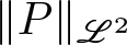 $\|P\|_{\mathscr{L}^2}$. Thus, as an additional check, in the bottom panel in Figure 4 we plot the estimate (11.2) for the nodal points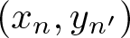 $(x_n,y_{n^\prime})$ we used in the domain region. Nodal points where the surface shown is positive indicate the potential number of decimal places lost at that nodal point. Across the whole domain region, the maximum this estimate reaches is roughly $2$, indicating that this phenomenon is only a minor contribution in our error estimates and analysis.
For analytic scattering data kernels, the exponential convergence of the GLM-CC and Det-CC methods, based on Bornemann’s [Reference Bornemann15] work, marks these methods out as extremely powerful tools in the simulation of  $KP$ solutions. These methods warrant further investigation. Furthermore, Bornemann’s comprehensive analysis reveals that the order of convergence is linearly related to the smoothness of the scattering kernel. Of interest in this direction is, given initial data for $g$ with only a certain degree of smoothness, to solve the scattering problem to generate the corresponding initial scattering data. This can be evolved forward in time to $t \gt 0$ in Fourier space via fast Fourier transform. This would result in a scattering data kernel at time $t$, of limited smoothness. Then we would apply the GLM-CC and/or Det-CC methods to generate the corresponding $KP$ solution at time $t \gt 0$. This is future work.
Acknowledgements
The authors acknowledge the helpful contribution of the late Henry McKean, who drew attention to the development potential of Pöppe’s work. We are also grateful to the referee, whose insightful comments improved this paper.


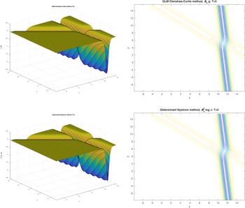


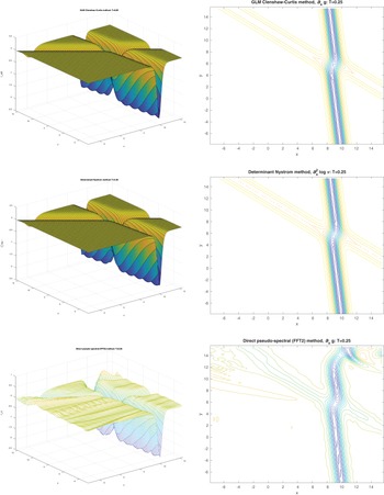


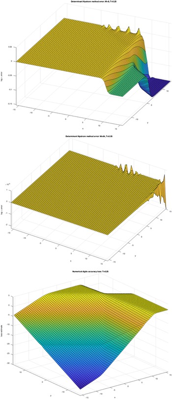


 Open access

