
1. Executive Summary
1.1 Overview
Under the European Union Solvency II regulations, insurance firms are required to calculate a one-year Value at Risk (VaR) of their balance sheet to a 1 in 200 level. This involves a one-year projection of a market-consistent balance sheet and requires sufficient capital to be solvent in 99.5% of outcomes. In order to calculate one-year 99.5th percentile VaR, a significant volume of one-year non-overlapping data is needed. In practice there is often a limited amount of relevant market data for market risk calibrations and an even more limited reliable and relevant data history for insurance/operational risks.
Two of the key issues with the available market data are:
The dataset available may be relatively longer (e.g. for corporate credit spread risk, Moody’s default and downgrade data are available from 1919Footnote 1 ), but data may not be directly relevant or not granular enough for risk calibration.
Dataset may be very relevant to the risk exposure and granular as required, but data length is not sufficient, for example, for corporate credit spread risk, Merrill Lynch or iBoxx data are available from 1996 or 2006, respectively.
As a consequence, practitioners need to make expert judgements about whether to:
use overlapping data or non-overlapping data (If overlapping data is used, then is there any adjustment that can be made to the probability distribution calibrations and statistical tests to ensure that the calibration is still fit for purpose?) or
use non-overlapping data with higher frequency than annual (e.g. monthly) and extract the statistical properties of this data which can allow us to aggregate the time series to lower-frequency (e.g. annual) time series.
In section 3 of this paper we consider adjustments to correct for bias in probability distributions calibrated using overlapping data. In section 4 adjustments to statistical tests are defined and tested. In section 5, issues with using data periods shorter than a year and then aggregating to produce annualised calibrations are considered.
1.2 Calibrating Probability Distributions Using Overlapping Data
Section 3 discusses the issues of probability distribution calibration using overlapping data. Adjustments to probability distribution calibrations using overlapping data in academic literature are presented and tested in a simulation study. We analysed the impact on cumulant bias and mean squared error (MSE) for some of the well-known statistical processes, namely Brownian, normal inverse Gaussian (special case of Levy process), ARMA, and GARCH processes under both overlapping and non-overlapping data approaches. We have analysed the impact on cumulants after applying corrections outlined by Sun et al. (Reference Sun, Nelken, Han and Guo2009) and Cochrane (Reference Cochrane1988). The simulation study involves producing computer-generated data and comparing the different approaches to estimating the known values of cumulants.
Cumulants are similar to moments and are properties of random variables. The first three cumulants – mean, variance, and skewness – are well known and the same as the first three central moments. The fourth cumulant is the fourth central moment minus 3*variance^2. Cumulants (and derived moments) are widely used in calibrating the probability distribution using method-of-moments-style calibration approaches. As with moments, cumulants uniquely define the calibration of a probability distribution within particular parameterised distribution families.
The key conclusions from the simulation study for the processes outlined above are:
Using published bias adjustments, both overlapping and non-overlapping data can be used to give unbiased estimates of statistical models where monthly returns are not autocorrelated. Where returns are autocorrelated, bias is more complex for both overlapping and non-overlapping data.
In general, overlapping data are more likely to be closer to the exact answer than non-overlapping data. By using more of the available data, overlapping data generally give cumulant estimates with lower MSE than using non-overlapping data.
1.3 Statistical Tests Using Overlapping Data
In section 4, we define and test an adjustment to a statistical test to allow for overlapping data.
To test whether a probability distribution fitted to a dataset is a good fit to the data, it is common to apply a statistical test. Many statistical tests have an assumption that the underlying data are independent, which is clearly not the case for overlapping data.
Using the Kolmogorov Smirnov (KS) statistical test, an adjustment is proposed to this test to allow for overlapping data. This adjustment is tested using simulated data and the results presented.
The test results indicate that the proposed adjustment for overlapping data to the KS test has a rejection rate consistent with test functioning as intended.
1.4 Alternative to Annual Data
An alternative to annual data is to use higher-frequency “monthly” data and then “annualise” it (i.e. convert the results from monthly data into annual data). Issues with this approach are considered in section 5. Higher-frequency data have the advantages of having more data points and no issues with overlapping data. The main disadvantage is that non-annual data need to be annualised, which comes with its own limitations. We have considered the following possible solutions:
Use of non-overlapping monthly data and annualising using empirical correlation that is present in the time series (see section 5.2 for further details). The key points to note from the use of annualisation are:
This technique involves:
○ fitting a probability distribution to monthly data;
○ simulating a large computer-generated dataset from this fitted model/distribution; and
○ aggregating the simulated monthly returns into annual returns using a copula or other relevant techniques.
It utilises all the data points and therefore would not miss any information that is present in the data; and in absence of information on the future, data trends would lead to a more stable calibration overall.
In the dataset we explored, it improves the fits considerably in comparison to non-overlapping data or monthly annual overlapping data because of the large simulated data used in the calibration.
However, it does not remove the autocorrelation issue completely (as monthly non-overlapping data or, for that matter, any “high”-frequency data could be autocorrelated) and does not handle the issues around volatility clustering.
Use of statistical techniques such as “temporal aggregation” (section 5.3). The key points to note from the use of temporal aggregation are:
Temporal aggregation involves fitting a time series model to monthly data, then using this time series model to model annual data.
It utilises as much data as possible without any key events being missed.
It improves the fit to the empirical data and leads to a stable calibration.
It can handle data with volatility clustering and autocorrelation.
However, it suffers from issues such as possible loss of information during the increased number of data transformations and is complex to understand and communicate to stakeholders.
Use of autocorrelation adjustment (or “de-smoothing” the data). This technique is not covered here as this is a widely researched topic (Marcatoo, Reference Marcatoo2003). However, a similar technique by Sun et al. (Reference Sun, Nelken, Han and Guo2009) has been used in section 3, which corrects for bias in the estimate of data variance.
1.5 Conclusions
The key messages concluded from this paper are:
There is a constant struggle between finding relevant data for risk calibration and sufficient data for robust calibration.
Using overlapping data is acceptable for Internal Model calibration; however, communication of uncertainty in the model and parameters to the stakeholder is important.
There are some credible alternatives to using overlapping data such as temporal aggregation and annualisation; however, these alternatives bring their own limitations, and understanding of these limitations is key to using these alternatives. We recommend considering the comparison of calibration using both non-overlapping monthly data annualised with overlapping annual data and discussing the advantages, robustness, and limitations of both the approaches with stakeholders before finalising the calibration approach.
1.6 Future Work
Further efforts are required in the following areas:
Diversification benefit using internal models is one of the key discussion topics among industry participants. So far, we have only analysed univariate time series. Further efforts are required in terms of analysing the impact of overlapping data on covariance and correlation properties between two time series.
Similarly, the impact on statistical techniques such as dimension reduction techniques (e.g. PCA) needs investigation. Initial efforts can be made in terms of treating each dimension as a single univariate time series and applying various techniques such a temporal aggregation or annualisation and applying dimension reduction techniques on both overlapping and non-overlapping transformed datasets to understand the impact.
The impact on statistical tests other than the KS test has not been investigated. We have also not investigated using different probability distributions than the normal distribution for the KS test. Both these areas could be investigated further using the methods covered in this paper.
Measurement of parameter and model uncertainty in the light of new information has not been investigated either for “annualisation” method or for “temporal aggregation” method.
2. Overlapping Data: Econometric Literature Survey
Within the finance literature, many authors have confronted the issue of data scarcity with which to calibrate a multi-period econometric model. Several approaches have been developed that justify the use of historic observation periods that are overlapping. These approaches extend classical statistical theory, which often presumes that the various observations are independent of each other. It is often the case that naïve statistics (constructed ignoring the dependence structure) are consistent (asymptotically tend towards true parameters) like their classical counterparts, but the standard errors are larger.
Hansen and Hodrick (Reference Hansen and Hodrick1980) examined the predictive power of 6-month forward foreign exchange rates. The period over which a regression is conducted is 6 months – yet monthly observations are readily available but clearly dependent. The authors derived the asymptotic distribution of regression statistics using the Generalised Method of Moments (GMM; Hansen Reference Hansen1982) which does not require independent errors. The regression statistics are consistent, and GMM provides a formula for the standard error. This approach has proved influential, and several estimators have been developed for the resulting standard error: Hansen and Hodrick’s original, Newey and West (Reference Newey and West1987), and Hodrick (Reference Hodrick1992) being prominent examples. Newey and West errors are the most commonly used in practice.
However, the derived distribution of fitted statistics is only true asymptotically, and the small-sample behaviour is often unknown. Many authors use bootstrapping or Monte Carlo simulation to assess the degree of confidence to attach to a specific statistical solution. For example, one prominent strand of finance literature has examined the power of current dividend yields to predict future equity returns. Ang and Bekaert (Reference Ang and Bekaert2006) and Wei and Wright (Reference Wei and Wright2013) show using Monte Carlo simulation that the standard approach of Newey and West errors produces a test size (i.e. probability of a type I error) which is much worse than when using Hodrick (1992) errors.
In addition to the asymptotic theory, there has also been work on small-sample behaviour. Cochrane (1988) examines the multi-year behaviour of a time series (GNP) for which quarterly data are available. He calculates the variance of this time series using overlapping time periods and computes the adjustment factor required to make this calculation unbiased in the case of a random walk. This adjustment factor generalises the n−1 denominator Bessel correction in the non-overlapping case. Kiesel, Perraudin and Taylor (Reference Kiesel, Perraudin and Taylor2001) extend this approach to third and fourth cumulants.
Müller (Reference Müller1993) conducts a theoretical investigation into the use of overlapping data to estimate statistics from time series. He concludes that while the estimation of a sample mean is not improved by using overlapping rather than non-overlapping data, if the mean is known, then the standard error of sample variance can be reduced by about 1/3 when using overlapping data. His analysis of sample variance is extended to the case of unknown mean, again with improvements of about 1/3, by Sun et al. (Reference Sun, Nelken, Han and Guo2009). Sun et al. also suggest an alternative approach of using the average of non-overlapping estimates. Like Cochrane and Müller, this leads to a reduction in variance of about 1/3 compared to using just non-overlapping data drawn from the full sample.
Efforts have been made to understand the statistical properties and/or behaviour of the “high”-frequency (e.g. monthly or daily data points) time series data to transform these into “low”-frequency time series data (i.e. annual data points) via statistical techniques such as temporal aggregation. Initial efforts were made to understand the temporal aggregation of ARIMA processes, and Amemiya and Wu (Reference Amemiya and Wu1972) led the research in this area. Feike_Drost_Nijman (Reference Drost and Nijman1993) developed closed-form solutions for temporal aggregation of GARCH processes and described relationships between various ARIMA processes under “high”-frequency and their transformation under “low”-frequency time series. Chan et al. (Reference Chan, Cheung, Zhang and Wu2008) show various aggregation techniques using equity returns (S&P500 data) and its impact on real-life situations.
The method of moments is not the only, and not necessarily the best, method for fitting distributions to data, with maximum likelihood being an alternative. There are some comparisons within the literature; we note the following points:
Maximum likelihood produces asymptotically efficient (lowest MSE) parameter estimates, while in general the method of moments is less efficient.
Model misspecification is a constant challenge, whatever method is used. Within a chosen distribution family, the moments may determine a distribution, but other distributions with the same moments, from a different family, may have different tail behaviour. For moment-based estimates, Bhattacharya’s inequality constrains the difference between two distributions with shared fourth moments, while, as far as we know, there are no corresponding results bounding misspecification error for maximum likelihood estimates.
The method of moments often has the advantage of simpler calculation and easy verification that a fitted distribution indeed replicates sample properties.
The adaptation of the maximum likelihood method to overlapping data does not seem to have been widely explored in the literature, while (as we have seen) various overlapping corrections have been published for method-of-moments estimates. For this reason, in the current paper, we have focused on moments/cumulants.
3. Simulation Study: Overlapping Versus Non-overlapping
3.1 Background
In this section, the results from a simulation study of the bias and MSE present in cumulant estimation using annual overlapping and non-overlapping data are presented. Cumulants are similar to moments (the first three cumulants are the mean, variance, and skewness and are exactly the same for moments); further information about cumulants is given in Appendix A.
Using a methodology outlined in Jarvis et al. (Reference Jarvis, Sharpe and Smith2017), monthly time series data are simulated from a known distribution (reference model) for a given number of years. The first four cumulants based on annual data are then calculated by considering both non-overlapping annual returns as well as overlapping annual returns (overlapping by 11 out of 12 months). By comparing the results of these with known cumulant values of the reference model and averaging across 1000 simulations, the bias and MSE of the estimates can be compared. This study is carried out using four different reference models:
Brownian process
Normal inverse Gaussian process
ARMA process
GARCHFootnote 2 process
A high-level description of this process is:
Simulate a monthly time series of n years data from one of the four processes above.
Calculate annual returns using overlapping and non-overlapping data.
Calculate the first four cumulants of annual returns (for overlapping and non-overlapping data).
Compare the estimated cumulants with known cumulants.
Repeat 1000 times to estimate the bias and MSE of both overlapping and non-overlapping data.
The analysis has been carried out for all years up to year 50, and the results are shown below. The results for ARMA and normal inverse Gaussian are in Appendix B.
3.2 Brownian Process Results
This section shows the bias and MSE for the first four cumulants.
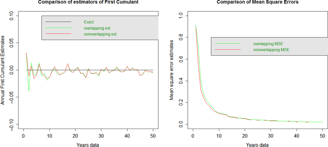
3.2.1 First cumulant: mean
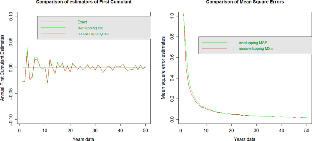
The diagram shows the bias in the plot on the left and the MSE on the plot on the right. The overlapping and non-overlapping data estimates of the mean appear very similar and not obviously biased. These also have very similar MSE across all years.
3.2.2 Second cumulant: variance
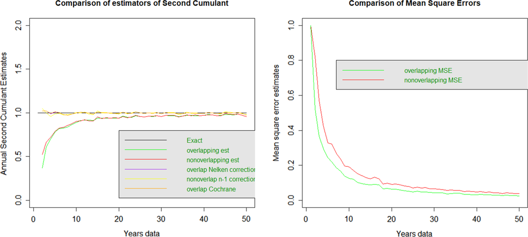
The second cumulant is variance (with divisor n).
The plot on the left shows that the overlapping and non-overlapping estimates of variance (with divisor n) are too low with similar bias levels for all terms. This is more marked, the lower the number of years data, and the bias appears to disappear as n gets larger.
The plot on the left also shows the second cumulant but bias-corrected, using a divisor (n−1) instead of n for the non-overlapping data and using the formula in Sun et al. as well as the Cochrane adjustment (Cochrane, 1988) for overlapping data. Both these corrections appear to have removed the bias across all terms for overlapping and non-overlapping data.
The plot on the right shows the MSE for the two approaches, with overlapping data appearing to have lower MSE for all terms.
3.2.3 Third cumulant
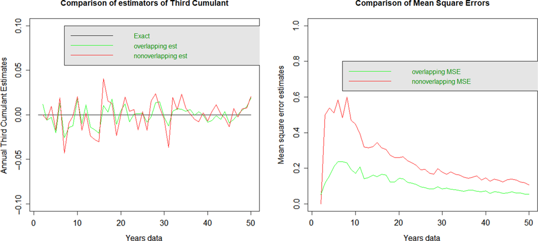
Neither approach appears to have any systemic bias for the third cumulant. The MSE is significantly higher for non-overlapping data than overlapping data.
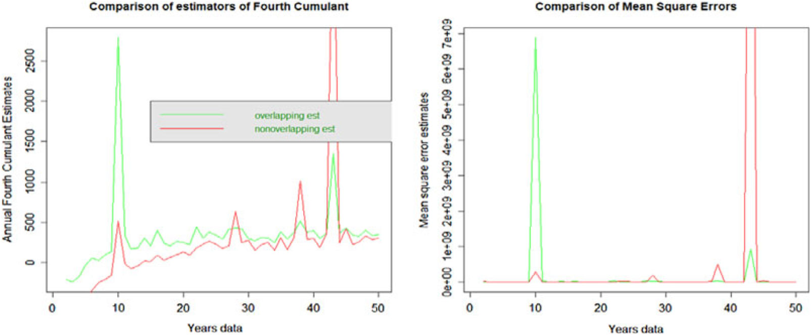
3.2.4 Fourth cumulant

In this case the non-overlapping data appear to have a higher downward bias than overlapping data at all terms; both estimates appear biased. The non-overlapping data have higher MSE than the overlapping data.
Plots of the bias and MSE for the normal inverse Gaussian are given in Appendix B. These are very similar to those of the Brownian process.
3.3 GARCH Results
3.3.1 First cumulant: mean

The diagram shows the bias in the plot on the left and the MSE on the plot on the right. The overlapping and non-overlapping data estimates of the mean appear very similar after 20 years. Below 20 years, the data show some bias under both overlapping and non-overlapping data series. These have very similar MSEs after 10 years, and below 10 years, non-overlapping data have marginally lower MSEs.
3.3.2 Second cumulant: variance
The second cumulant is variance (with divisor n).

Both approaches have similar levels of bias, particularly when available data are limited. Bias corrections now both overstate the variance particularly strongly for datasets with less than 10 years data. The MSE for overlapping data appears to be materially lower than non-overlapping data.
3.3.3 Third cumulant

The non-overlapping data have both higher bias and MSE compared to overlapping data across all years.
3.3.4 Fourth cumulant
The non-overlapping data have lower bias compared to overlapping data. However, overlapping data have lower MSE.
3.4 Discussion of Simulation Results
The results above show the bias and MSE for the first four cumulants of each of the reference distributions.
For the first cumulant, the results are similar for all four reference distributions tested. There is no obvious bias for either non-overlapping or overlapping data series. The MSE of overlapping and non-overlapping data series is at a similar level for both. These results show that for the estimation of the first cumulant, both approaches perform similarly on the bias and MSE tests, and there is no need for any correction for bias.
For the second cumulant, the results vary for different reference models.
For the Brownian and normal inverse Gaussian reference models, the non-overlapping and overlapping data series are both downwardly biased to a similar extent. In both cases bias can be corrected for by using the Bessel correction for non-overlapping data, and the Cochrane (1988) or Sun et al. (Reference Sun, Nelken, Han and Guo2009) corrections for overlapping data. The MSE is lower for the overlapping data (due to the additional data included). These results suggest that for the estimation of the second cumulant, the overlapping data perform better due to lower MSE and have a greater likelihood to be nearer to the true answer.
4. Statistical Tests Using Overlapping Data
In this section the use of statistical tests with overlapping data is discussed. An adjustment to a statistical test to allow for the use of overlapping data is proposed. This adjustment is then tested using computer-generated data.
4.1 Statistical Tests
When fitting a probability distribution to a dataset, it is common practice to assess its goodness of fit using a statistical test, such as the chi-squared test (Bain & Engelhardt, Reference Bain and Engelhardt1992, p. 453), Anderson Darling test (Bain & Engelhardt, Reference Bain and Engelhardt1992, p. 458) or, in the case of this paper, the KS test (Bain & Engelhardt, Reference Bain and Engelhardt1992, p. 460).
The KS test is based on calculating the largest Kolmogorov distance, which is the distance between a single data point and the point’s projected position on the probability distribution fitted to the data.
The KS test is intended to compare the underlying data against the distribution the data came from where the parameters are known. If the parameters themselves tested against in the KS test have been estimated from the data, this introduces sample error. This sample error is not allowed for in the standard KS test, and a sample error adjustment is required which, in the case of a normal distribution, is known as Lillifors adjustment (Conover, Reference Conover1999).
A description of this adjustment for sampling error for data from a normal distribution is given below:
1. Fit a normal distribution to the dataset of n data points and calculate the parameters for normal distribution.
2. Measure the Kolmogorov distance for the fitted distribution and the dataset, call this D.
3. Simulate n data points from a normal distribution with the same parameters as found in step 1. Re-fit another normal distribution and calculate the Kolmogorov distance between this newly fitted normal and the simulated data.
4. Repeat step 3 1000 (or suitably large) times to generate a distribution of Kolmogorov distances.
5. Calculate the percentile the distance D is on the probability distribution calculated in step 4.
6. If the distance D is greater than the 95th percentile of the probability distribution calculated in step 4, then it is rejected at the 5% level.
The reason this approach works is because the KS distance is calculated between the data and a fitted distribution and then compared with 1000 randomly generated such distances. If the distance between the data and the fitted distribution is greater than 95% of the randomly generated distances, then there is statistically significant evidence against the hypothesis that the data are from the fitted distribution.
4.2 Adjustment for Overlapping Data
If overlapping data are used instead of non-overlapping data, then even if the non-overlapping data are independent and identically distributed, the overlapping data will not be, as each adjacent overlapping data point will be correlated. This means overlapping data will not satisfy the assumptions required of most statistical tests, such as the KS test.
However, it is possible to adjust most statistical tests to allow for the use of overlapping data. A method for doing so is shown here for the KS test. The approach used is similar to that described above to correct for sampling error, except that both the data being tested and the data simulated as part of the test are overlapping data. The steps are:
1. Fit a normal distribution to the dataset of n overlapping data points and calculate the parameters for normal distribution.
2. Measure the Kolmogorov distance for the fitted distribution and the dataset, call this D.
3. Simulate n overlapping data points from a normal distribution with the same parameters as found in step 1. Re-fit another normal distribution and calculate the Kolmogorov distance between this newly fitted normal and the simulated data.
4. Repeat step 3 1000 times to generate a distribution of Kolmogorov distances.
5. Calculate the percentile the distance D is on the probability distribution calculated in step 4.
6. If the distance D is greater than the 95th percentile of the probability distribution calculated in step 4, then it is rejected at the 5% level.
A key question is how to simulate the overlapping data in step 3 in the list above. For Levy-stable processes such as normal distribution, this can be done by simulating from the normal distribution at a monthly timeframe and then calculating the annual overlapping data directly from the monthly simulated data. For processes which are not Levy-stable, an alternative is to directly simulate annual data and then aggregate into overlapping data using a Gaussian copula with a correlation matrix which gives the theoretical correlation between adjacent overlapping data points, where the non-overlapping data are independent. This approach generates correlated data from the non-Levy-stable distribution, where the correlations between adjacent data points are in line with theoretical correlations for overlapping data. (This last approach is not tested below.)
This adjustment works for the same reason as the adjustment described in section 4.1. The KS distance is generated between the data and the fitted distribution. This distance is then compared with 1000 randomly generated distances, except this time using overlapping data. If the distance between the data and the fitted distribution is greater than 95% of the randomly generated distances, then there is statistically significant evidence against the hypothesis that the data are from the fitted distribution.
4.3 Testing the Adjustments to the KS Test Using Simulated Data
Using the same testing approach applied in section 3, defined in Jarvis et al. (Reference Jarvis, Sharpe and Smith2017), the KS test and the adjustments described above have been assessed. This approach to testing involves simulating data from known distributions, then fitting a distribution to the data, carrying out a statistical test and then assessing the result of the test against the known correct answer.
The tests carried out are:
1. Test of the standard KS test. This is done using non-overlapping simulated data from a normal distribution with mean 0 and standard deviation 1.
a. 100 data points are simulated from this normal distribution.
b. The KS test is carried out between this simulated data and the normal distribution with parameters 0 for mean and 1 for standard deviation.
c. The p-value is calculated from this KS test.
d. Steps a, b, and c are repeated 1000 times and the number of p-values lower than 5% are calculated and divided by 1000.
2. Test of the KS test with sample error. This test is done using non-overlapping simulated data from a normal distribution with mean 0 and standard deviation 1. The difference between this test and test 1 is that step b in test 1 is using known parameter values, whereas this test uses parameters from a distribution fitted to the data.
a. 100 data points are simulated from this normal distribution.
b. The normal distribution is fitted to the data using the maximum likelihood estimate (MLE).
c. The KS test is carried out between the simulated data and the fitted normal distribution.
d. The p-value is calculated for this KS test.
e. Steps a, b, c and d are repeated 1000 times and the number of p-values lower than 5% are calculated and divided by 1000.
3. Test of the KS test with correction for sample error. This test is done using non-overlapping simulated data from a normal distribution with mean 0 and standard deviation 1. The difference between this test and test 2 is that step c is carried out using the KS test adjusted for sample error.
a. 100 data points are simulated from this normal distribution.
b. The normal distribution is fitted to the data using the MLE.
c. The KS test adjusted for sample error (as described in section 4.1) is carried out between the simulated data and the fitted normal distribution.
d. The p-value is calculated for this KS test.
e. Steps a, b, c, and d are repeated 1000 times and the number of p-values lower than 5% is calculated and divided by 1000
4. Test of the KS test with correction for sample error applied to overlapping data. This test is done using overlapping simulated data from a normal distribution with mean 0 and standard deviation 1. The difference between this test and test 3 is that the simulated data in this test is from an overlapping dataset.
a. 100 data points are simulated from this normal distribution.
b. The normal distribution is fitted to the data using the MLE.
c. The KS test adjusted for sample error (as described in section 4.1) is carried out between the simulated data and the fitted normal distribution.
d. The p-value is calculated for this KS test.
e. Steps a, b, c, and d are repeated 1000 times and the number of p-values lower than 5% are calculated and divided by 1000.
5. Test of the KS test with correction for sample error applied to overlapping data, and correction for overlapping data (as described in 5.2). This test is done using overlapping simulated data from a normal distribution with mean 0 and standard deviation 1. The difference between this test and test 4 is that the KS test corrects for overlapping data as well as sample error.
a. 100 data points are simulated from this normal distribution.
b. The normal distribution is fitted to the data using the MLE.
c. The KS test adjusted for sample error (as described in section 4.1) is carried out between the simulated data and the fitted normal distribution. This was done with a reduced sample size of 500 in the KS test to improve run times.
d. The p-value is calculated for this KS test.
e. Steps a, b, c, and d are repeated 500 times and the number of p-values lower than 5% are calculated and divided by 500.
4.4 Results of the Simulation Study on the KS Test
The results of the simulation study are the rejection rate for each statistical test. For data generated randomly from a known distribution tested against a 5% level, we would expect a 5% rejection rate. The results from each of the tests described in section 4.3 are:

4.5 Discussion of Results
This section discusses each of the test results presented in section 4.4.
For test 1, the test assesses the rejection rate for the standard KS test applied as it is intended to be applied (i.e. compared against known parameter values). The result of 4.3% compares to an expected result of 5%. This may indicate the standard KS has a degree of bias.
For test 2, the test assesses the rejection rate for the KS test applied using the sample fitted parameters with no allowance for sample error. The rejection rate of 0% indicates that if sample error is not corrected for, there is almost no chance of rejecting a fitted distribution.
For test 3, the KS test is now corrected for sample error, and the rejection rate of close to 5% indicates the KS test with sample error correction is working as intended.
For test 4, the KS test with the sample error correction is applied to overlapping data. The rejection rate is very high at 44% relative to an expected 5% level. This indicates that applying the KS test with sample error correction to overlapping data will have a much higher rejection rate than expected.
For test 5, the KS test with sample error and overlapping error correction is applied to overlapping data. The 5.3% result of this test (closely in line with the expected rate of 5%) indicates the overlapping error correction is working as expected.
This test shows it is possible to achieve a rejection rate in line with expectations by adjusting the KS test for overlapping data as described in section 4.2.
5. Using Periods Shorter than Annual Data
So far, we have discussed the issues with using overlapping data for the purpose of risk calibration and possible methods of correcting for the overlapping data, including the adjustments made to the data as covered in sections 3 and 4.
Alternatively, the industry participants have tried to use “high”-frequency data (e.g. monthly or quarterly data) to get to “low”-frequency data (e.g. annual data) to meet the Solvency II requirements of performing a 1-in-200 year calibration over a one-year period.
In this section, we consider the issues around these alternative approaches where time periods shorter than one year are used to derive the annual calibration. This avoids some of the problems with using overlapping data directly, considered in sections 3 and 4. An example of this approach is to fit a model to monthly data, then extend this same model to also model annual returns.
The approaches discussed in this section can be considered possible alternatives to using annual non-overlapping and/or monthly annual overlapping data. The uncertainties present in the approaches discussed in this section are also considered.
5.1 Approaches Using Data Periods Shorter Than Annual
Three possible approaches to using data periods shorter than a year for the calibration of VaR at an annual time frame are:
Use of non-overlapping monthly data but annualising these using autocorrelation that is present in the time series (section 5.2)
○ This technique involves fitting a probability distribution to monthly data, simulation from a large computer-generated dataset from this fitted distribution, and aggregating the simulated monthly returns into annual returns using a copula and the correlation.
○ It utilises all the data points and leads to a stable calibration.
○ It improves the fit considerably in comparison to non-overlapping data or monthly annual overlapping data.
○ However, it does not remove the autocorrelation issue completely and does not handle the issues around volatility clustering.
Use of statistical techniques such as “temporal aggregation” (section 5.3)
○ It involves fitting a time series model to monthly data, then using this time series model to model annual data.
○ It annualises the monthly data systematically in line with the monthly time series model fitted to the monthly data.
○ It utilises as much data as possible without any key events being missed.
○ It improves the fit to the empirical data and leads to a stable calibration.
○ It can handle the data with volatility clustering and avoids the issue of autocorrelation.
Use of autocorrelation adjustment (or “de-smoothing” the data)
○ This technique is not covered here as this is a widely researched topic (Marcatoo, Reference Marcatoo2003). However, we have tried using a similar technique by Sun et al. (Reference Sun, Nelken, Han and Guo2009), which tries to correct the bias in the overlapping variance of the data. We have analysed the impacts of using this adjustment in section 3 of the paper and have not discussed it further in this section.
The testing carried out in section 5 is based on empirical data where the underlying model driving the data is unknown. As the model is unknown, the bias and MSE tests carried out in section 3 are not possible (as these require the model parameters to be known).
5.2 Annualisation Method
Under this approach, we analyse the data points using monthly non-overlapping time steps but utilise the correlation present in the monthly time series data to create a large dataset to perform an annual non-overlapping calibration.
The key data analysis steps are as follows:
Calculate the monthly changes in the time series.
Calculate empirical correlation between each of the 12 calendar months by arranging all January changes in one column and February changes in the next one and so on and calculate the correlations.
Apply this correlation to generate a large number of monthly steps (e.g. 100 k) and aggregate monthly steps to come up with annualised simulations depending upon whether we are modelling the time series multiplicatively or additively.
Annualisation is performed using empirical marginal distributions and a Gaussian (or even empirical) copula using an autocorrelation matrix for each of the time series to avoid any information loss due to fitting errors.
This technique has the advantage of fitting distributions based on a large sample leading to more stable results. However, it suffers from the fact that it still uses monthly data which may be autocorrelated.
We fit distributions to these annualised simulations. We present the use of this technique using Merrill Lynch (ML) credit data, where we compare the results of using annual overlapping data (without any aggregation approach) and using the above autocorrelation aggregation approach.
5.2.1 Dataset used
Although the methodology used for annualisation is quite generic in nature and can be used for a wide range of datasets, we have used ML credit indices because of the following peculiarities of this dataset:
The dataset is limited (starting in 1996) and therefore the utilisation of information available in each of the data points is important.
This dataset has a single extreme market event (2008–2009 global credit crisis) and the rest of the data are relatively benign.
Two significant challenges for calibrating this dataset are:
○ If we use an annual non-overlapping dataset, we may lose the key events of 2008–2009 global credit crisis where the extreme movements in spreads happened during June 2008–March 2009 (a nine-month period).
○ If we use an annual overlapping dataset, the data points used in the fitting process are more than the data points using an annual non-overlapping dataset, but not sufficient for generating a credible and robust fit at the 99.5th percentile point.
5.2.2 Empirical data analysis
In this section, the main purpose is to compare the results of some of the general tests applied to both annual overlapping and monthly non-overlapping data to check whether using monthly non-overlapping time series is more conducive to risk calibration or not.
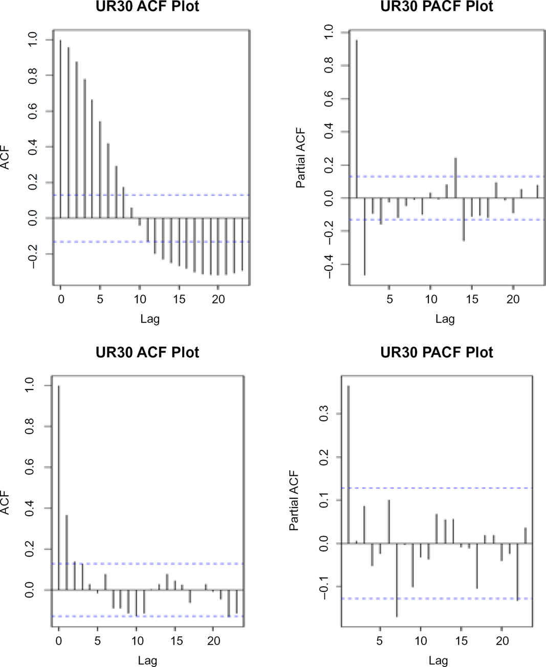
We consider a practical example of the approach described in the previous section based on credit spread data. We first look at the autocorrelation function (ACF) and partial autocorrelation function (PACF) plotsFootnote 3 using two of the ML credit indices: UR30 (ML A-rated index – all maturities) and UR40 (ML BBB-rated index – all maturities), see Figures 1 and 2. The term annual overlapping is used in this section to mean annual data overlapping by 11 out of 12 months of the year.
Annual overlapping versus monthly non-overlapping – a RATING – all maturities. Under the annual overlapping time series (top left) the ACF starts at 1, slowly converges to 0 (slower decay) and then becomes negative and exceeds the 95% confidence level for the first nine lags. Under the monthly non-overlapping time series (bottom left) the ACF quickly falls to a very low number, and beyond lag 2 for most time lags, the autocorrelations are within the 95% confidence interval. For all practical purposes we can ignore the ACF after time lag 2. The suggests that using monthly non-overlapping time series is less autocorrelated than the annual overlapping time series. Similarly, the PACF for monthly non-overlapping data (bottom right) shows more time steps where autocorrelations beyond lag 2 are within the 95% confidence interval in comparison to the annual overlapping data (top right). The purpose of performing these tests is to show if using monthly non-overlapping time series is more conducive to modelling or not.
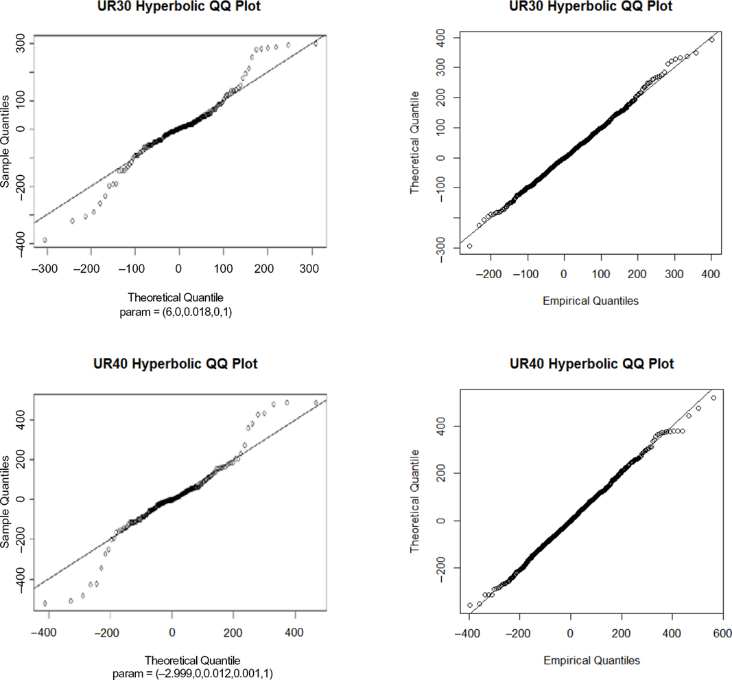
Annual overlapping versus monthly non-overlapping with autocorrelation. From the QQ plots (both using the hyperbolic distribution) between monthly annual overlapping and monthly non-overlapping with annualisation, it is clear that using monthly non-overlapping data with autocorrelation appears to improve the fits in the body as well as in the tails. This is because the QQ plots show a much closer fit to the diagonal for the monthly non-overlapping data with annualisation. Note: We used the hyperbolic distribution as it is considered one of the most sophisticated distributions. Similar conclusions can be drawn using more simpler distributions, such as the normal distribution.
The autocorrelation plots show the correlation between data points with different lags on the x-axis. Similarly, for the partial autocorrelation plots also show relationship between data points with different lags on the x-axis. Note that stationarity tests have been carried out in Appendix C.
5.2.2.1 Fitting results: QQ plots – hyperbolic distribution
We present the QQ plots for annual overlapping versus monthly non-overlapping with autocorrelation using hyperbolic distribution.
5.2.2.2 Conclusions
Annualising monthly non-overlapping data using monthly autocorrelations can be a versatile alternative to annual overlapping data, particularly where data are limited. It is important to note that annualisation is not always the ideal solution because it also introduces uncertainty depending upon the aggregation approach used. However, this uncertainty can be reduced by using empirical distributions for the high-frequency data (i.e. monthly process) where possible and using empirical or Gaussian copula where the minimum number of parameter estimations are required in annualisation.
5.3 Temporal Aggregation Methods
Another alternative approach to using overlapping annual data is to use temporal aggregation, as shown in Table 1. This is an approach where we construct a low-frequency series (e.g. annual series) from a high-frequency series (e.g. monthly/daily series). This is done by fitting a time series model (e.g. auto-regressive, GARCH, etc.) to the monthly data, which then gives all the information required to model the annual time series.
Key quantiles: monthly annualised versus monthly annual overlapping data

Temporal aggregation can be very useful in cases where we have limited relevant market data available for calibration and we want to infer the annual process from the monthly/daily process.
5.3.1 Introduction
Under the temporal aggregation technique, the low-frequency data series is called the aggregate series (e.g. annual series), as shown in Table 2. The high-frequency data series is called the disaggregate series (e.g. monthly series). Deriving a low-frequency model from the high-frequency model is a two-stage procedure:
ARMA-GARCH models are given in terms of lag polynomials, where it is necessary to choose the polynomial orders. Temporal aggregation allows us to infer the orders of the low-frequency model from those of high frequency.
After inferring the orders, the parameters of the low-frequency model should be recovered from the high-frequency ones, rather than estimating these. Hence, the low-frequency model parameters incorporate all the economic information from the high-frequency data.
 $$Y_t^{\rm{\ast}} = W\left( L \right){y_t} = \mathop \sum \limits_{j = 0}^A {w_j}{y_{t - j}} = \mathop \sum \limits_{j = 0}^{k - 1} {L^j}{y_t}$$
where W(L) is the lag polynomial of order A. W(L) = 1 + L + … + LΛ (k−1), where k represents the order of aggregation.
Table of parameters

If the disaggregate time series yt were to follow a model of the following type,
 $${\emptyset} \left( L \right){y_t} = \theta \left( L \right){\varepsilon _t}$$
where ∅(L) and θ (L) are lag polynomials and ϵt is an error term, then the temporally aggregated time series can be described by
 $$\beta \left(B\right)y_t^{\ast} = \phi \left( B \right)\varepsilon_t^{\ast}$$
We perform a time series regression model to estimate the coefficients of an ARMA or ARIMA model on monthly non-overlapping data.
Annual estimates are constructed out of non-overlapping monthly observations.
Autocorrelation in the data is accounted for to make sure the estimates are valid.
The standard goodness-of-fit techniques are valid.
The key limitations of temporal aggregation are as follows:
Temporal aggregation leads to a loss of information in the data when performing various data transformations. However, empirical work done using equity risk data shows that this loss of information has not been materially significant based on the quantile results observed under various approaches in section 5.3.2.
Rigorous testing and validation of the behaviour of residuals will be necessary. It is complex to understand and communicate.
The main complication with using temporal aggregation technique is the fact that it involves solving an algebraic system of equations, which can get complex for complex time series models of higher orders, for example, ARIMA (p,d,q), where p, d, and/or q exceed 3.
5.3.1.1 Technical details for AR(1) process
We study this technique using a simple auto-regressive AR(1) process. Assume that the monthly log-return rt follows an AR(1) process (Chan et al., Reference Chan, Cheung, Zhang and Wu2008).
 $${r_t} = \emptyset \ {r_{t - 1}} + {a_t},{\rm{}}{a_t}\sim N\left( {0,\sigma _a^2} \right)$$
The annual returns are noted as RT and frequency is defined as m (where m = 12 for annual aggregation). The lag-s auto-covariance functions of the m-period aggregated log return variable.
 $$Cov\left[ {{R_T},{\rm{}}{R_{T + s}}} \right] = \left[ {m + 2\left( {m - 1} \right) + 2\left( {m - 2} \right){\emptyset ^2} + .. + 2{\emptyset ^{m - 1}}} \right]{\rm{}}{{\sigma _a^2} \over {1 - {\emptyset ^2}}} \ if \ s = 0$$
 $$Cov\left[ {{R_T}, \ {R_{T + s}}} \right] = \left[ {1 + \emptyset + {\emptyset ^2} + .. + {\emptyset ^{m - 1}}} \right]\left[ {{{{\emptyset ^{m\left( {\left| s \right| - 1} \right) + 1}}} \over {1 - {\emptyset ^2}}}} \right]\sigma _a^2 \ if \ s = \pm 1, \pm 2.$$
 $$Var\left[ {{R_T}} \right] = \left[ {12 + 22 + 20{\emptyset ^2} + .. + 2{\emptyset ^{11}}} \right]{{\sigma _a^2} \over {1 - {\emptyset ^2}}} \ when \ s = 0 \ and \ m = 12$$
 $$\left( {1 - {\emptyset ^{\rm{\ast}}}L} \right){R_T} = \left( {1 - {\theta ^{\rm{\ast}}}L} \right)a_t^{\rm{\ast}}\,a_t^{\rm{\ast}} \sim \ N\left( {0,\sigma _{{a^{\rm{\ast}}}}^2} \right)$$
Ø* = Øm (for real-life applications where for annualisation we use Ø12; it will be close to zero and therefore the process essentially becomes an MA (1) process). For |Ø*| < 1,
 $$\eqalign{ ({\emptyset ^m} - {\theta ^{\rm{\ast}}}) & {{\left( {1 - {\emptyset ^m}{\theta ^{\rm{\ast}}}} \right)} \over {1 - 2{\emptyset ^m}{\theta ^{\rm{\ast}}} + {\theta ^{{\rm{\ast}}2}}}} \cr & = \emptyset {\left[ {1 + \emptyset + {\emptyset ^2} + .. + {\emptyset ^{m - 1}}} \right]^2}/\left[ {m + 2\left( {m - 1} \right) + 2\left( {m - 2} \right){\emptyset ^2} + .. + 2{\emptyset ^{m - 1}}} \right]}$$
5.3.1.2 Technical details for GARCH (1, 1) process
Let at = (rt - μ) be a mean-corrected log-return and follow GARCH (1,1) process, then
 $${\varepsilon _t} = {\rm{}}{a_t}/h_t^{0.5}$$
 $${h_t} = {\rm{}}\omega + {\rm{}}\beta {h_{t - 1}} + \alpha a_{t - 1}^2$$
The m-month non-overlapping period can be “weakly” approximated by GARCH (1,1) process with corresponding parameters:
 $${\mu ^{\rm{\ast}}} = m\mu$$
 $${\omega ^{\rm{\ast}}} = m\omega \left\{ {{{1 - {{\left( {\alpha + \beta } \right)}^m}} \over {1 - \left( {\alpha + \beta } \right)}}} \right\}$$
 $${\alpha ^{\rm{\ast}}} = {\left( {\alpha + \beta } \right)^m} - {\rm{}}{\beta ^{\rm{\ast}}}$$
|β*| < 1 is a solution of the following quadratic equation:
 $${{{\beta ^{\rm{\ast}}}} \over {1 + {\rm{}}{\beta ^{\rm{\ast}}}^2}} = {{\left( {{\rm{\Theta }}{{\left( {\alpha + \beta } \right)}^m} - {\rm{\Lambda }}} \right)} \over {\left( {{\rm{\Theta }}{{\left( {1 + (\alpha + \beta } \right)}^{2m}}) - 2{\rm{\Lambda }}} \right)}}$$
 $${\rm{\Lambda }} = \left( {{{\left( {\alpha - \alpha \beta \left( {\alpha + \beta } \right)} \right)\left( {1 - {{\left( {\alpha + \beta } \right)}^{2m}}} \right)} \over {1 - {{\left( {\alpha + \beta } \right)}^2}}}} \right)$$
 $${\rm{\Theta }} = m{\left( {1 - \beta } \right)^2} + \left\{ {{{2m\left( {m - 1} \right){{\left( {1 - \alpha - \beta } \right)}^2}\left( {1 - 2\alpha \beta - {\beta ^2}} \right)} \over {\left( {\kappa - 1} \right)\left( {1 - {{\left( {\alpha + \beta } \right)}^2}} \right)}}} \right\} + 4\left\{ {{{\left( {m - 1 - m\left( {\alpha + \beta } \right) + {{\left( {\alpha + \beta } \right)}^m}} \right)\left( {\alpha - \alpha \beta \left( {\alpha + \beta } \right)} \right)} \over {1 - {{\left( {\alpha + \beta } \right)}^2}}}} \right\}$$
where κ is the unconditional kurtosis of the data.
 $${\kappa ^{\rm{\ast}}} = 3 + {{\kappa - 3} \over m} + 6\left( {\kappa - 1} \right)\left\{ {{{\left( {\alpha - \alpha \beta \left( {\alpha + \beta } \right)} \right)\left( {m - 1 - m\left( {\alpha + \beta } \right) - {{\left( {\alpha + \beta } \right)}^m}} \right)} \over {{m^2}{{\left( {1 - \alpha - \beta } \right)}^2}\left( {1 - 2\alpha \beta - {\beta ^2}} \right)}}} \right\}$$
5.3.2 UK equity temporal aggregation – GARCH (1,1)
In this section, we present an example of the temporal aggregation method applied to the UK (FTSE All Share Total Return) index data using the GARCH model fitted to monthly data.
The calculation steps applied are as follows:
Calculate excess of mean log monthly non-overlapping returns of the data.
Fit a GARCH (1,1) model to these excess of mean log returns and derive the fitted parameters of GARCH model.
Calculate the temporally aggregated parameters for the annual time series.
Compare the (simple) quantiles of empirical annual non-overlapping, empirical annual overlapping, and temporally aggregated GARCH (1,1) process.
From a comparison of the key quantiles, we conclude:
On the extreme downside and upside, temporally aggregated GARCH (1,1) process leads to stronger quantiles in comparison to annual non-overlapping and annual overlapping time series.
In the “body” of the distribution, temporally aggregated GARCH (1,1) process leads to weaker quantiles in comparison to annual non-overlapping and monthly annual overlapping time series.
The calibration parameters of GARCH (1, 1) process fitted to monthly non-overlapping and temporally aggregated GARCH (1, 1) are outlined in Table 2.
6. Conclusions
This paper has considered some of the main issues with overlapping data as well as looking at the alternatives.
Section 3 presented the results of a simulation study designed to test whether overlapping or non-overlapping data are better for distribution fitting. For the models tested, overlapping data appear to be better as biases can be removed (in a similar way to non-overlapping data), but overlapping makes a greater use of the data, meaning it has a lower MSE. A lower MSE suggests that distributions fitted with overlapping data are more likely to be closer to the correct answer.
Section 4 discussed the issues of statistical tests using overlapping data. A methodology was tested and the adjustment for overlapping data was found to correct the statistical tests in line with expectations.
Section 5 presented alternative methods for model fitting, by fitting the model to shorter time frame data and then aggregating the monthly model into an annual model. This approach was successfully tested in a practical example.
The overall conclusions from this paper are:
Overlapping data can be used to calibrate probability distributions and is expected to be a better approach than using non-overlapping data, particularly when there is a constant struggle between finding relevant data for risk calibration and maximising the use of data for a robust calibration. However, communication of the uncertainty in the model and/or parameters to the stakeholder is equally important.
Some credible alternatives exist to using overlapping data such as temporal aggregation and annualisation. However, these alternatives bring their own limitations, and understanding these limitations is key to using these alternatives. We recommend considering a comparison of calibration using both non-overlapping monthly data annualised with overlapping annual data, and discussing with stakeholders the advantages, robustness, and limitations of both the approaches before finalising the calibration approach.
Appendix A
In this section, we provide the mathematical definitions and descriptions of technical terms used in the paper.Footnote 4
A.1 What Are Cumulants of a Random Variable?
A.1.1 Definitions
Cumulants are properties of random variables. The first two cumulants – mean and variance – are well known. The third cumulant is also the third central moment. For a random variable X with mean µ, the first four cumulants are:
 $${\kappa _1} = \mu = {E} \left( X \right)$$
 $${\kappa _2} = {E} {\left( {X - \mu } \right)^2}$$
 $${\kappa _3} = {E}{\left( {X - \mu } \right)^3}$$
 $${\kappa _4} = {E}{\left( {X - \mu } \right)^4} - 3\kappa _2^2$$
Higher cumulants theoretically exist but are less often encountered. We restrict our discussion to first four cumulants only.
A.2 Statistical Properties of Cumulants
A.2.1 Additive property
The cumulants satisfy an additive property for independent random variables. If X and Y are statistically independent and n ≥ 1, then
 $${\kappa _n}\left( {X + Y} \right) = {\kappa _n}\left( X \right) + {\kappa _n}\left( Y \right)$$
For a normal distribution, the third and subsequent cumulants are zero.
A.2.2 Skewness and kurtosis
Skewness and kurtosis of a random variable are defined in terms of cumulants, as follows:
 $$\rm{Skewness} = {{{\kappa _3}} \over {\kappa _2^{3/2}}}$$
 $$\rm{Kurtosis} = {{{\kappa _4}} \over {\kappa _2^2}}$$
Skewness and kurtosis are both shape attributes, which are unchanged when a random variable is shifted or scaled by a positive multiple.
It is a consequence of the additive property that, for sums of independent identically distributed random variables, skewness and kurtosis tend to zero as the number of observations in the sum tends to infinity. This observation is consistent with the central limit theorem.
A.3 Using Cumulants to Estimate Distributions
A.3.1 Empirical cumulants
Given a number n of data points, empirical distribution puts a mass of n –1 on each observation.
The empirical cumulants are cumulant estimates based on the empirical distribution, which we denote with a tilde (∼). The first empirical cumulant ${\tilde k_1}$
is the sample average. Other empirical cumulants are defined similarly. For example, empirical variance (second cumulant) is the average squared deviation between each observation and that sample average. The empirical fourth moment
${\tilde k_1}$
is the sample average. Other empirical cumulants are defined similarly. For example, empirical variance (second cumulant) is the average squared deviation between each observation and that sample average. The empirical fourth moment ${\tilde k_4}$
is the average fourth power of deviations, minus three times the squared empirical variance.
${\tilde k_4}$
is the average fourth power of deviations, minus three times the squared empirical variance.
A.3.2 Distribution fitting with cumulants
We can use empirical cumulants, or modifications thereof, to estimate distributions. The methodology is to find a distribution whose cumulants match the cumulants estimated from a data sample (i.e. as with the method of moments, a probability distribution is uniquely defined by its cumulants).
A common practice (see EEWP 2008; Willis Towers Watson [WTW]Footnote 5 risk calibration survey 2016) for market risk models is to pick a four-parameter distribution family, closed under shifting and scaling. EEWP 2008 showed distributions from the Pearson IV family and the hyperbolic family. In this paper we show examples based the normal inverse Gaussian family. In each case, the procedure is the same:
- Estimate the mean, variance, skewness, and kurtosis from the historical data.
- Pick a four-parameter distribution family.
- Evaluate whether the estimated (skew, kurtosis) combination is feasible for the chosen family. If not, adjust the historical values by projecting onto the boundary of the feasible region.
- Find the distribution matching the adjusted historical skewness and kurtosis.
- Match the mean and variance by shifting and scaling.
- Compare the fitted distribution to the historic data, either by inspection of histograms or more formal statistical tests. If the fit is not good enough, then think of another four-parameter family and repeat from the third step above.
Appendix B: Simulation Study – Additional Results
This section shows additional results from the simulation study in section 3.
B.1 Normal Inverse Gaussian Results
The results for the normal inverse Gaussian reference model are shown below. These results are very similar to the Brownian case.
B.1.1 First moment: mean
The plots show the bias in the plot on the left and the MSE on the plot on the right. The overlapping and non-overlapping data estimates of the mean appear very similar and not obviously biased. These also have very similar MSE across all years. This has very similar conclusions to the Brownian case.
B.1.2 Second cumulant: variance

The second cumulant is the variance (with divisor n). This has very similar conclusions to the Brownian case.
Overlapping and non-overlapping data both give biased estimates of the second cumulant to a similar extent across all terms.
The bias correction factors (using divisor n−1 for non-overlapping variance and the Nelken formula for overlapping variance) appear to remove the bias. This is evidence that the Nelken bias correction factor works for other processes than just Brownian motion.
The plot on the right shows the MSEs for the two approaches, with overlapping data appearing to have lower MSE for all terms.
B.1.3 Third cumulant

Neither approach appears to have any systemic bias for the mean. The MSE is significantly higher for non-overlapping data than for overlapping data.
B.1.4 Fourth cumulant

In this case the non-overlapping data appear to have a higher downward bias than the overlapping data at all terms; both estimates appear biased. The bias does not appear to tend to zero as the number of years increases, but it rises above the known value. The non-overlapping data have higher MSE than the overlapping data.
B.2 ARIMA Results
B.2.1 First cumulant: mean

The plots show the bias in the plot on the left and the MSE on the plot on the right. The overlapping and non-overlapping data estimates of the mean appear very similar and unbiased. These also have very similar MSEs after 10 years, but overlapping data appear to have marginally higher MSE below 10 years.
B.2.2 Second cumulant: variance

The plot on the left shows that the overlapping and non-overlapping estimates of variance (with divisor n) are too low with similar bias levels for all terms. This is more marked, the lower the number of years data, and the bias appears to disappear as n gets larger.
The plot on the left also shows the second cumulant but bias-corrected, using a divisor (n−1) instead of n for the non-overlapping data and using the formula in Sun et al. as well as in Cochrane (1988) for the overlapping data. Both these corrections appear to have removed the bias across all terms for overlapping and non-overlapping data. The MSE is very similar for both overlapping and non-overlapping data.
B.2.3 Third cumulant

It is important to note that neither approach appears to have any materially different bias. Non-overlapping data have higher MSE compared to overlapping data.
B.2.4 Fourth cumulant

Non-overlapping data have lower bias compared to overlapping data, but overlapping data have lower MSE.
Appendix C: Stationarity Tests
C.1 Phillips–Perron (PP) Test (Phillips & Perron, Reference Phillips and Perron1988)
The PP test involves fitting the following regression model:
 $${y_t} = {\rm{}}\alpha + \rho {y_{t - 1}} + \delta t + {u_t}$$
The results are used to calculate the test statistics proposed by Phillips and Perron. Phillips and Perron’s test statistics can be viewed as Dickey–Fuller statistics that have been made robust to serial correlation by using the Newey–West (1987) heteroskedasticity- and autocorrelation-consistent covariance matrix estimator. Under PP unit root test, the hypothesis is as follows:
H null: The time series has a unit root (which means it is non-stationary).
H alternative: The time series does not have a unit root (which means it is stationary).
C.2 Kwiatkowski–Phillips–Schmidt–Shin (KPSS) Test (Kwiatkowski et al., Reference Kwiatkowski, Phillips, Schmidt and Shin1992)
The KPSS test has been developed to complement unit root tests as the latter have low power with respect to near-unit root and long-run trend processes. Unlike unit root tests, Kwiatkowski et al. provide straightforward test of the null hypothesis of trend and level stationarity against the alternative of a unit root.
For this, they consider the three-component representation of the observed ADF time series as the sum of a deterministic time trend, a random walk, and a stationary residual:
 $${Y_t} = \beta t + \left( {{r_t} + \alpha } \right) + {e_t}$$
= rt
= rt−1
+ μt is a random walk, the initial value r
0 = α serves as an intercept, t is the time index, ut
are independent identically distributed (0, $\sigma _u^2$
). Under the KPSS test, the hypothesis is as follows:
$\sigma _u^2$
). Under the KPSS test, the hypothesis is as follows:
H null: The time series is trend/level stationary (which means it does not show trends).
H alternative: The time series is not trend/level stationary (which means it does show trends).
C.3 Ljung-Box Q Test (Ljung & Box, Reference Ljung and Box1978)
The Ljung-Box Q test is whether any of a group of autocorrelations of a time series are different from zero. Instead of testing randomness at each distinct lag, it tests the “overall” randomness based on a number of lags, and is therefore a portmanteauFootnote 6 test. Under the Ljung-Box Q test, the hypothesis is as follows:
H null: The time series is independent.
H alternative: The time series is not independent and has a positive or negative strong serial correlation.
The statistic under the Ljung-Box test is calculated as follows:
 $$Q = n\left( {n + 2} \right)\mathop \sum \limits_{k = 1}^h {{\hat \rho _k^2} \over {n - k}}$$
where n is the sample size, $\hat \rho _k^2$
is the sample autocorrelation at lag k, and h is the number of lags being tested. Under the null hypothesis,
$\hat \rho _k^2$
is the sample autocorrelation at lag k, and h is the number of lags being tested. Under the null hypothesis, $Q\sim \chi _h^2$
, where h is the degree of freedom.
$Q\sim \chi _h^2$
, where h is the degree of freedom.
These tests have been applied to corporate bond indices with the results presented in Table C.1.
Credit indices: monthly non-overlapping data – stationarity and unit root tests

The credit spread data is subject to a number of different stationarity tests. If the process is stationary, it is more conducive for a robust calibration because its statistical properties remain constant over time (e.g. the mean, variance, autocorrelation, etc., do not change). If the process is not stationary, the variation in the fitting parameters can be significant as the new information emerges in the new data, or in some cases the model may no longer remain valid. This point is important for stakeholders because the stability of the SCR depends upon the stability of risk calibrations.
There are various definitions of stationarity in the literature. We present a “weak” stationarity definition here. We believe it is widely used; however, stronger forms may be required, for example, when considering higher moments.
A process is said to be covariance stationary or “weakly stationary” if its first and second moments are time-invariant, that is,
 $$E\left( {{Y_t}} \right) = E\left( {{Y_{t - 1}}} \right) = \mu {\rm{}}\forall t$$
 $$Var\left( {{Y_t}} \right) = {\gamma _0} \lt \infty \forall t$$
 $$Cov\left( {{Y_t},{\rm{}}{Y_{t - k}}} \right) = {\gamma _k} \lt \infty \forall t,{\rm{}}\forall k$$
The third condition means that the auto-covariances only depend on time decay but not in the time itself. Hence, the structure of the series does not change with time.
The results of a number of statistical tests for stationarity together with a discussion of these results are presented in Table C.2.
PP and KPSS tests

The key implications of these tests are:
The stationarity tests support (or are unable to reject) the hypothesis that the time series are stationary under both monthly non-overlapping annualised data and monthly annual overlapping data.
It is important to note that the Ljung-Box test suggests that the data have serial correlation for monthly annual overlapping data. However, we are able to reject the hypothesis for monthly non-overlapping annualisation approach.
The purpose of doing these tests is to show that using monthly non-overlapping annualised data can be a better alternative if we can annualise it rather than using monthly annual overlapping data.


 Open access