


1. Introduction
Meltwater processes on Antarctic ice shelves are influenced by the permeability of surface snow and firn. Ponding of meltwater above impermeable shallow ice has been implicated as a precursor to ice shelf collapse (Banwell, Reference Banwell2017). Understanding the extent of impermeable zones within firn – so-called ‘ice slabs’ – is therefore important for hydrological modelling and subsequent predictions of the long-term stability of the ice shelves that fringe Antarctica. The formation and subsequent freezing of meltwater on (and within) ice shelves reduces firn permeability, causing the formation of surface meltwater ponds (Munneke and others, Reference Munneke, Ligtenberg, van den Broeke and Vaughan2014; Bevan and others, Reference Bevan2017). These in turn influence ice shelf stability by promoting hydrofracture, a process that has been associated with the 2002 collapse of Larsen B ice shelf (Scambos and others, Reference Scambos, Bohlander, Shuman and Skvarca2004). As ice shelves buttress ice streams, they restrict the transfer of ice from terrestrial ice sheets into the ocean. When the buttressing is removed following collapse, feeder glaciers and ice streams accelerate and can increase the contribution of terrestrial glaciers to sea-level rise (Wuite and others, Reference Wuite2015). As patterns of melt and refreezing change (Rintoul and others, Reference Rintoul2018), it is expected that the presence of ice slabs within snow-covered regions will become more prevalent, including in Antarctica. There is therefore an important and growing need to characterise ice slabs within firn.
Ice slabs form over several cycles of thaw and refreeze, when pre-existing ice layers within firn coalesce. Ice slabs form in locations where surface melt occurs, including the coastal regions of Antarctica and Greenland. With a lateral extent of tens-to-hundreds of meters, ice slabs make the shallow firn column impermeable (Benson, Reference Benson1962; MacFerrin and others, Reference MacFerrin2019; Miller and others, Reference Miller2022) and can increase its local density from 400 to 800 kg m–3 (typical of firn) to that of pure glacier ice, 917 kg m−3 (e.g. Hubbard and others, Reference Hubbard2016; MacFerrin and others, Reference MacFerrin2019; Culberg and others, Reference Culberg, Schroeder and Chu2021). Radar data from IceBridge AR flight lines from 2010 to 2014 show that ice slabs covered 64 800–69 400 km2 of the Greenland ice sheet in 2014, ~4% of the ice sheet's total area (MacFerrin and others, Reference MacFerrin2019). Greenland's ice slabs have been predicted to increase in area by 130–850% by 2100 depending on the level of 21st century CO2 emissions (MacFerrin and others, Reference MacFerrin2019). Without explicitly accounting for the effects of ice slabs, meltwater runoff can be underestimated, for example, in Greenland, regional climate models suggest runoff to be underestimated by almost 60% if ice slab formation is excluded (MacFerrin and others, Reference MacFerrin2019; Lai and others, Reference Lai2020).
Seismic reflections and refractions in ice are caused by any process that changes its elastic properties, including density, bulk and shear moduli, viscosity and anisotropy (Diez and others, Reference Diez, Eisen, Hofstede, Bohleber and Polom2013; Schlegel and others, Reference Schlegel2019), which in turn modify the velocity of compressional (P) and shear (S) seismic energy (Aki and Richards, Reference Aki and Richards2002). Consequently, seismic methods have broad applicability in glaciology for imaging the internal and underlying structure of glaciers and ice masses (e.g. Diez and others, Reference Diez2016; Brisbourne and others, Reference Brisbourne2019; Church and others, Reference Church2019; Riverman and others, Reference Riverman2019), but are increasingly used to quantify glacier physical properties (e.g. density, water content, etc.; Endres and others, Reference Endres, Murray, Booth and West2009; Booth and others, Reference Booth2012; Peters and others, Reference Peters, Anandakrishnan, Alley and Voigt2012; Macchioli-Grande and others, Reference Macchioli-Grande, Zyserman, Monachesi, Jouniaux and Rosas- Carbajal2020), temperature from changes in anisotropy (e.g. Lutz and others, Reference Lutz, Eccles, Prior and Hulbe2019; Llorens and others, Reference Llorens2020) and characterise the properties of snow and firn from seismic data (e.g. Kohnen and Bentley, Reference Kohnen and Bentley1973; Kinar and Pomeroy, Reference Kinar and Pomeroy2007; Bradford, Reference Bradford2010; Diez and others, Reference Diez2014; Schlegel and others, Reference Schlegel2019).
Seismic methods have been applied to characterise the density structure of firn, using seismic velocity as a proxy for density (e.g. Kirchner and Bentley, Reference Kirchner and Bentley1979; King and Jarvis, Reference King and Jarvis1991, Reference King and Jarvis2007; Booth and others, Reference Booth2013; Hollmann and others, Reference Hollmann, Treverrow, Peters, Reading and Kulessa2021). As the degree of firn compaction increases, so too do density and elastic moduli, leading to an increase in seismic velocity. When an ice slab is present within a firn column, the contrast in seismic velocity between that ice and the adjacent firn can be used to diagnose the presence, bulk properties and thickness of that ice slab.
A commonly used approach for characterising seismic velocity trends in firn from controlled-source seismic data is the Herglotz–Wiechert inversion (HWI) (Herglotz, Reference Herglotz1907; Wiechert, Reference Wiechert1910; Slichter, Reference Slichter1932; Nowack, Reference Nowack1990) in which a velocity-depth model is evaluated from the slowness (the reciprocal of velocity) of seismic arrivals (e.g. Thiel and Ostenso, Reference Thiel and Ostenso1961; Diez and others, Reference Diez, Eisen, Hofstede, Bohleber and Polom2013; Godio and Rege, Reference Godio and Rege2015). Though popular in glaciology, a key assumption in HWI is that seismic velocity must increase with depth, which is violated when ice slabs are present in the firn column – specifically across the lower boundary of the slab (or multiple slabs), where material transitions back into unmodified firn. When HWI is applied to regions with ice slabs, slab boundaries are improperly represented due to the limitations of the technique, leading to an incorrect velocity structure above, within and below the ice slab (Aki and Richards, Reference Aki and Richards2002).
These limitations can be overcome by the use of seismic full waveform inversion (FWI) methods. FWI extends the capacities of HWI by using both the slowness and amplitude information in the seismic dataset, thereby matching the recorded seismic wavefield rather than just the travel time of arrivals. For the case of ice slabs, which present a seismic velocity reduction at their base, FWI is in principle sensitive to this velocity structure and hence offers the potential to determine slab thickness. Furthermore, HWI methods consider only the travel time of first arrivals in a seismic dataset, whereas FWI can also access later refracted arrivals and the reflections from the bounding interfaces of the ice slabs.
Unlike ray-based methods, which consider only the travel time of first arrivals, FWI considers finite-frequency wave propagation and evaluates velocity models using the amplitude and travel time of the recorded wavefield. Therefore, the resolution of FWI is only limited by the source and receiver distribution, noise level and scales with the seismic wavelength (Williamson, Reference Williamson1991; Schuster, Reference Schuster2017; Pratt and others, Reference Pratt, Gao, Zelt and Levander2002; Warner and others, Reference Warner2013). Babcock and Bradford (Reference Babcock and Bradford2014) provided the first glaciological application of FWI to characterise subglacial seismic velocities in the presence of seismically ‘thin’ layering (i.e. less than ¼ wavelength, typically ~10 m; Widess, Reference Widess1973; Smith, Reference Smith2007; Booth and others, Reference Booth2012). The study reported encouraging results, in particular in terms of improving the accuracy of recorded compressional (P-) wave velocities.
Here, we explore the scope of FWI methods to recover firn velocity structures that are currently unresolvable with HWI. We first compare FWI and HWI for synthetic seismic data that model steady-state firn accumulation profiles, where HWI results should be reliable. The performance of FWI is then considered for seismic velocity models corresponding to firn with ice slab inclusions.
For steady-state firn cases, we show that outputs from FWI are no less accurate than conventional HWI, but are greatly superior for any non-steady state firn profile in which ice slabs are present.
2. Inversion approaches
2.1 Herglotz–Wiechert inversion
HWI produces a 1-D velocity structure in which velocity must increase with depth. In the case of firn, this can be used to produce accurate velocity models for steady-state conditions, and has been used repeatedly to characterize firn structure in a variety of settings (e.g. Thiel and Ostenso, Reference Thiel and Ostenso1961; Diez and others, Reference Diez, Eisen, Hofstede, Bohleber and Polom2013; Godio and Rege, Reference Godio and Rege2015). This one-dimensional continuous velocity structure can be approximated by a stack of thin layers of constant velocity, which can be considered a suitable approximation for many firn structures. Following Snell's law, seismic energy incident at a boundary refracts and the ratio of the sine of the angle of incidence θn and the velocity in the nth layer, vn is constant, defining the horizontal slowness or ray parameter u.
For a monotonically increasing velocity, the ray parameter decreases monotonically, causing the ray to turn and to be recorded at the surface allowing sampling of the velocity structure. At the turning point, where the maximum depth (z max) of the propagation is reached, the refraction angle θ reaches 90° and the horizontal slowness is equal to the inverse of the velocity at this depth, allowing a mapping of seismic velocities using methods such as HWI.
To convert slowness to a depth/velocity domain, the HWI approach uses Abel's integral equation. From Bôcher (Reference Bôcher1909), the necessary and sufficient conditions that Abel's integral must meet are that the derivative of slowness (t(x)) can be discontinuous, but t(x) itself cannot be discontinuous (such as when dealing with velocity discontinuities and lateral velocity variations). For the travel time-offset data to be used successfully with the HWI, the travel time picks obtained from the first break arrival times of the seismic data must be smooth and continuous. Various algorithms exist for fitting a curve to the first break picks to achieve this, with the Levenberg–Marquardt algorithm being used here (Moré, Reference Moré2006; Kirchner and Bentley, Reference Kirchner and Bentley1979), as implemented by King and Jarvis (Reference King and Jarvis2007). The travel time, t, approximation is achieved through

with a 1, a 2, a 3 and a 4 being positive curve fitting parameters and a 5 is the inverse of the seismic velocity of ice.
Using Eqn (1) instead of the measured travel times ensures that travel time increases monotonically with distance (i.e. velocity increases monotonically with depth), and allows a solution using Abel's equation (Kirchner and Bentley, Reference Kirchner and Bentley1979). For each offset (x), the ray parameter (p) of the travel time curve can be determined and the depth (z) to the related velocity (as function of slowness u) can be determined using:

Once repeated for all offsets on the slowness offset curve, a smooth velocity-depth model is obtained (Nowack, Reference Nowack1990; Aki and Richards, Reference Aki and Richards2002).
2.2 Full waveform inversion
FWI delivers subsurface velocity models by minimising the misfit between observed and modelled seismic waveform data. The seismic wave equation is used to describe wave propagation in a medium and can be used to calculate synthetic seismic waveforms from a (starting) velocity model (Virieux and Operto, Reference Virieux and Operto2009; Babcock and Bradford, Reference Babcock and Bradford2014). The starting velocity model is updated through successive iterations that improve the match between predicted and observed data.
A solution to the inversion is found by matching the predicted seismic data to the observed data (d) trace by trace (Mulder and Plessix, Reference Mulder and Plessix2004; Warner and others, Reference Warner2013). This uses a non-linear local iterative minimisation scheme: in its simplest form, the misfit is characterised by a scalar value termed the objective function (Warner and others, Reference Warner2013). The most common form of the objective function (OF) is a least-squares (LS) formulation that minimises the sum of the square of the difference between the observed and predicted datasets.
Here we follow the approach of Aragao and Sava (Reference Aragao and Sava2020) who define the data residual as;

with the objective function then defined as

where a, x and t are, respectively, the experiment index, space coordinates and time, ||2 indicates the L2 (least-squares) norm, W u(a, x, t) are trace weights, es(a, x, t) the (synthetic) source wavefield and d(a, x, t) are the observed data. The model that minimises the objective function is considered to the best solution to the inversion (Pratt, Reference Pratt1999). We use a gradient-based method to update the model iteratively following the approach outlined in Aragao and Sava (Reference Aragao and Sava2020). For more information on the numerical approach, see the description there.
The FWI algorithm used in this study is based on the acoustic wave equation,

where p is pressure, v p is the propagation velocity of seismic compressional (P-) wave, and ρ is the density of the medium. The equation assumes isotropic wave propagation and no attenuation.
The acoustic wave equation is usually modelled with finite-difference (FD) methods, due to their simplicity and efficiency compared to other techniques available to solve partial differential equations (Virieux and Operto, Reference Virieux and Operto2009; Zhang and Yao, Reference Zhang and Yao2013). To simplify the source characterisation in the FD approach, the source model, a Ricker wavelet, is assumed with a peak frequency of 60 Hz and density is assumed to be a constant of 917 kg m−3. To ensure modelling stability, data are recorded with a time sampling of 0.001 s, for 1 s of propagation (Courant and others, Reference Courant, Friedrichs and Lewy1967).
Using a CPU Intel(R) Xeon(R) CPU E5-2690 0 at 2.90 GHz, forward modelling the data on two cores uses a total of 163 Mb of memory per seismic shot. Per seismic shot, each iteration run time is ~10 min on a single processor. So for the experiments shown here, the total run time was ~12 h.
Seismic wave propagation is described by the seismic wave equation containing the elastic properties of the subsurface. For relatively simple elastic (velocity) models, the seismic wave equation can be solved analytically. For more complex models, numerical solutions are necessary (Ben-Menahem and Singh, Reference Ben-Menahem and Singh2012; Guasch and others, Reference Guasch2012; Moczo and others, Reference Moczo, Kristek and Gális2014). Finite differences (FD) are a commonly used and stable method and has been found to provide computationally efficient and accurate solutions for a wide range of velocity structures (Virieux and Operto, Reference Virieux and Operto2009; Zhang and Yao, Reference Zhang and Yao2013).
FWI solutions can suffer from non-linearity and model non-uniqueness, and the technique can be computationally expensive. A particular problem is that of cycle-skipping, where modelled and recorded data are out of phase by half a wavelength, yet still offer a locally minimised objective function (Sirgue, Reference Sirgue2006) (Fig. 1). In such cases, FWI converges on a local, rather than global, minimum, which reduces the objective function but produces an incorrect velocity model. Cycle skipping can be exacerbated by data acquisition, survey geometry and the choice of inversion algorithm (Guasch and others, Reference Guasch2012; Shah and others, Reference Shah2012; Brittan and others, Reference Brittan, Bai, Delome, Wang and Yingst2013; Bai and Yingst, Reference Bai and Yingst2014; Jones, Reference Jones2015, Reference Jones2019; Borisov and others, Reference Borisov2017) and starting velocity model, which is selected carefully such that the first iteration of modelled data matches the observations to within half a wavelength. The risk of cycle skipping is mitigated by (i) using the low frequencies (i.e. long wavelengths) of the data which, due to their longer wavelength, are less prone to cycle skipping, and (ii) including far-offset data, which typically contain higher velocities and thus longer wavelengths (Sirgue and others, Reference Sirgue, Barkved, Van Gestel, Askim and Kommedal2009; Virieux and Operto, Reference Virieux and Operto2009; Al-Yaqoobi, Reference Al-Yaqoobi2013; Warner and others, Reference Warner2013).
Schematic representation of cycle skipping (adapted from Prajapati and Ghosh, Reference Prajapati and Ghosh2016). (a) If the initial modelled data and observed data are more than half a cycle away then (b) the data update to a local minimum, i.e. the modelled data are matched to the incorrect part of the observed data, in that the trailing-trough of the black curve coincides with the leading-trough of the red curve.

For the inversion, seismic propagation is modelled assuming an acoustic wave in a 2-D isotropic medium with no attenuation, with the recovered parameter being P-wave velocity. When calculating the residual, data are normalised by the maximum amplitude in each trace.
The misfit between recorded and modelled data is defined as the objective function (OF) given in Eqn (3). We use an adjoint method (Plessix, Reference Plessix2006) and a gradient-based method (Tarantola, Reference Tarantola, Aki and Wu1988) to update the model between iterations. We use the Madagascar framework (Fomel and others, Reference Fomel, Sava, Vlad, Liu and Bashkardin2013), provided by the Center for Wave Phenomena, to implement this approach (Aragao and Sava, Reference Aragao and Sava2020). To minimize the impact of cycle skipping, we start iterations for the low-frequency wavefield, filtered between 3 and 10 Hz, running a minimum of five iterations for each frequency band until the OF updates suggest model convergence. The chosen frequency band is representative of the lowest frequency feasibly recovered in glaciological field data from a hammer seismic source. Thereafter, the frequency content is progressively increased in 10 Hz bands, to a maximum of 60 Hz.
In our FWI, we use a gradient approach to define the fit between recorded and modelled data (Aragao and Sava, Reference Aragao and Sava2020). To minimise the OF with respect to the model parameters (m), the OF is differentiated,

This OF gradient indicates the direction of update of the model m in the next iteration in order to reduce the OF, with α a scaling factor known as the step length (Dai and Yuan, Reference Dai and Yuan1999).
In the proximity of the source and receivers, FWI gradient artefacts can occur due to the complex wavefield interactions caused by the near-field effects. These artefacts can lead to inaccurate subsurface images and hinder the convergence of the FWI algorithm. To mitigate these effects, we allow the non-linear solver to rebalance the amplitudes without the use of weighting due to the proximity of ice layers in the near surface in our velocity models.
3. Synthetic testing of FWI applicability
To validate the performance of FWI for realistic steady-state firn velocity profiles, firn density profiles are simulated using the Herron–Langway (HL) firn densification model (Herron and Langway, Reference Herron and Langway1980) and converted to velocity (Kohnen, Reference Kohnen1972). The HL model is based on the three stages of firn generation and uses snow accumulation rate and ambient temperature as input variables.
The HL model requires parameters to be chosen for total firn thickness, surface accumulation rate, surface snow density and the average temperature at 10 m depth. The chosen values (Table 1) for density (snow, ice and critical), and temperature are consistent with those of Herron and Langway (Reference Herron and Langway1980).
Parameterisation used for the Herron and Langway firn densification model

The accumulation value of 0.2 m water equivalent per year (m w.e. a−1) is used to represent a typical value for coastal Antarctica. It is generally accepted that higher accumulation rates produce thicker firn profiles, and thus gentler gradients of density and velocity increase (Herron and Langway, Reference Herron and Langway1980) (Fig. 2).
The synthetic seismic velocity profile obtained by converting the Herron and Langway densification profile with an accumulation rate of 0.2 m w.e. a−1 with the Kohnen (Reference Kohnen1972) approximation. From a depth of 0–25 m, the most gradual increase in velocity with depth is seen. Deeper than 25 m (where the critical density is reached) the densification, and hence velocity, rate increases. A maximum velocity of 3800 m s−1 is reached at 200 m depth.

The density profiles obtained from the HL model are converted to seismic velocity using the Kohnen (Reference Kohnen1972) approximation. A single seismic source is placed at 0 m offset, with surface receivers placed from 0 to 1000 m (five-times greater than the model depth) in one meter increments. This acquisition geometry is reflective of the offsets acquired in glaciological refraction surveys, using explosive or hammer source at the surface (e.g. Smith and others, Reference Smith, Jordan, Ferraccioli and Bingham2013; Brisbourne and others, Reference Brisbourne2020). We use a 2-D acquisition to recover a 1-D velocity profile from FWI, as horizontal velocity homogeneity is assumed.
Three analyses are performed using the synthetic firn velocity profiles. Firstly, the velocity model from the FWI is compared to the velocity model produced by the HWI, where the HWI model is used as the starting model for FWI. Secondly, we impose an increasing degree of systematic error to the true model to use as the starting velocity model for the FWI, to explore the extent to which FWI can resolve incorrect starting models. This will explore how a decreasing starting model accuracy affects the FWI update to the velocity model and the data. Finally, the third model simulates two different HL firn densification profiles (low and high accumulation of 0.1 and 0.4 m w.e. a−1, respectively), but uses the starting velocity model from the original profile (an accumulation of 0.2 m w.e. a−1). This explores whether FWI can distinguish different densification scenarios even when a ‘benchmark’ starting velocity profile is assumed.
Thereafter, the steady-state models are modified to introduce ice slabs into the firn profile. Assuming the density and velocity of an ice slab to be 917 kg m−3 and 3800 m s−1 (Cuffey and Paterson, Reference Cuffey and Paterson2010), these values are allocated to varied depth and thickness ranges of the firn profile to simulate the presence of ice slabs. We assess whether FWI is able to detect the velocity change at the upper and lower interfaces of the slab, and the extent to which it resolves the correct velocity model.
Velocity model outputs from FWI are compared to the true subsurface velocity model using the normalised root mean square error (NRMS), defined by Kragh and Christie (Reference Kragh and Christie2002) as

where RMS(V) and RMS(M) are the root-mean-square velocities of the true and predicted model.
The absolute percentage difference (DD) between the true and inverted velocity models is defined throughout the model with a depth interval of one meter. DD indicates how close the modelled velocity (Mzi) is to the true velocity (Vzi), calculated as;

4. Results
4.1 HWI of steady-state profiles
Data are forward modelled from the synthetic velocity model (true model). This produces the observed seismic dataset (Fig. 3a). From these observed data, travel times are extracted (Fig. 3b) and the HWI inversion is used to obtain an estimation of the subsurface velocity structure and compared to the true velocity model.
(a) Forward modelled, observed, synthetic data, where positive amplitudes are shaded. The first arrival is produced from the diving wave, while the second arrival is produced by the direct wave, travelling at the lowest velocity (the velocity at the surface) in the model (d) produced from the HL firn velocity model with an accumulation rate of 0.02 m w.e. a−1. Red traces show those enlarged in (b). (b) First break picks used as the input for Herglotz–Wiechert shown for selected offsets. (c) The output velocity model produced by the HWI (red) compared to the true HL firn velocity model (black).

In general, HWI provides a close representation of the velocity distribution of the steady-state firn profile. From 15 to 125 m, the velocity is recreated accurately, and the predicted velocity remains within 3% of the true model. For the shallowest depths, before the critical density is reached, HWI overestimates velocity. This is consistent with observations of Hollmann and others (Reference Hollmann, Treverrow, Peters, Reading and Kulessa2021), who suggested that HWIs are poorly constrained in the near-surface, with inaccuracies in first-break picking being proportionally greater at smaller travel times. Beyond 125 m depth, HWI underestimates velocity by 4%, converging on a velocity of ~3650 m s−1.
4.2 FWI of steady-state profiles
The output of the HWI (Fig. 3c) is used as a starting velocity model for FWI. Data are forward modelled from this starting velocity model to obtain a predicted seismic dataset, p′. Comparing the observed data (d) and p′ (Fig. 4), the first arrival is modelled accurately but the second arrival, the direct arrival produced by the direct wave travelling at the lowest velocity in the model, does not overlap with the observed data. This is evident in the red trace in Figure 4a: the second arrival in the predicted data (red) appears ~0.005 s earlier than in the model, suggesting that shallow velocities are being overestimated. This is also evident in Figure 4b, where the red-coloured second arrivals show a faster velocity trend than the observed data. This mismatch must be reduced to where the observed data and predicted data are within half a wavelength so a reduction in the objective function can be achieved by a change in the velocity model. This is a separate effect to cycle skipping, caused by a bad initial model, but must be addressed for FWI to produce reasonable updates to the velocity model.
(a) Comparison of seismic arrivals for trace 200 between the observed data (black), the predicted data (red) and predicted data from a constrained starting velocity model (blue). The data produced from the predicted (HWI) starting model are prone to cycle skipping in the second arrival, hence the adjusted HWI velocity model is used for a starting model with FWI.

The blue trace in Figure 4a shows the output from a modified starting model, which constrains the velocity in the uppermost one meter of the profile to the true model value (1023 m s–1). With this modification, both arrivals are now modelled within half a cycle of one another. This highlights the vulnerability of HWI and FWI to near-surface velocity errors, and points to the need for field acquisitions to constrain the shallowest velocities – either through a small-offset seismic refraction survey or a vertical seismic profile in a borehole or test pit.
Once the uppermost velocity is constrained, Figure 5 suggests that FWI can perform as reliably as the HWI that provided the starting model: the NRMS for both approaches is ~1.4%.
(a) The output of FWI on the constrained HWI starting model, shown for trace 200. (b) Velocity model output from FWI compared to the starting model (red) and true model (black), expressed as NRMS and the percentage error between the two output models (HWI and FWI) and the true model.

To explore the sensitivity of FWI to velocity errors, the starting velocity model is perturbed from its true value by up to ±10%. This generates eight further starting models. Figure 6 shows examples of FWI performance where the starting model is overestimated by 2.5% (A and C) and 10% (B and D). The analysis indicates that FWI is robust for the 2.5% error, but cycle skips for the case of the 10% error (Fig. 7).
(a, b) The velocity models produce by FWI for a starting model that is a 2.5% overestimation and 10% overestimation of the true model. (c, d) The seismic data for trace 200 for the same starting models respectively. The overestimation of 10% still enables the near offset traces to be matched, but the amplitude is not correctly accounted for with the acoustic FWI.
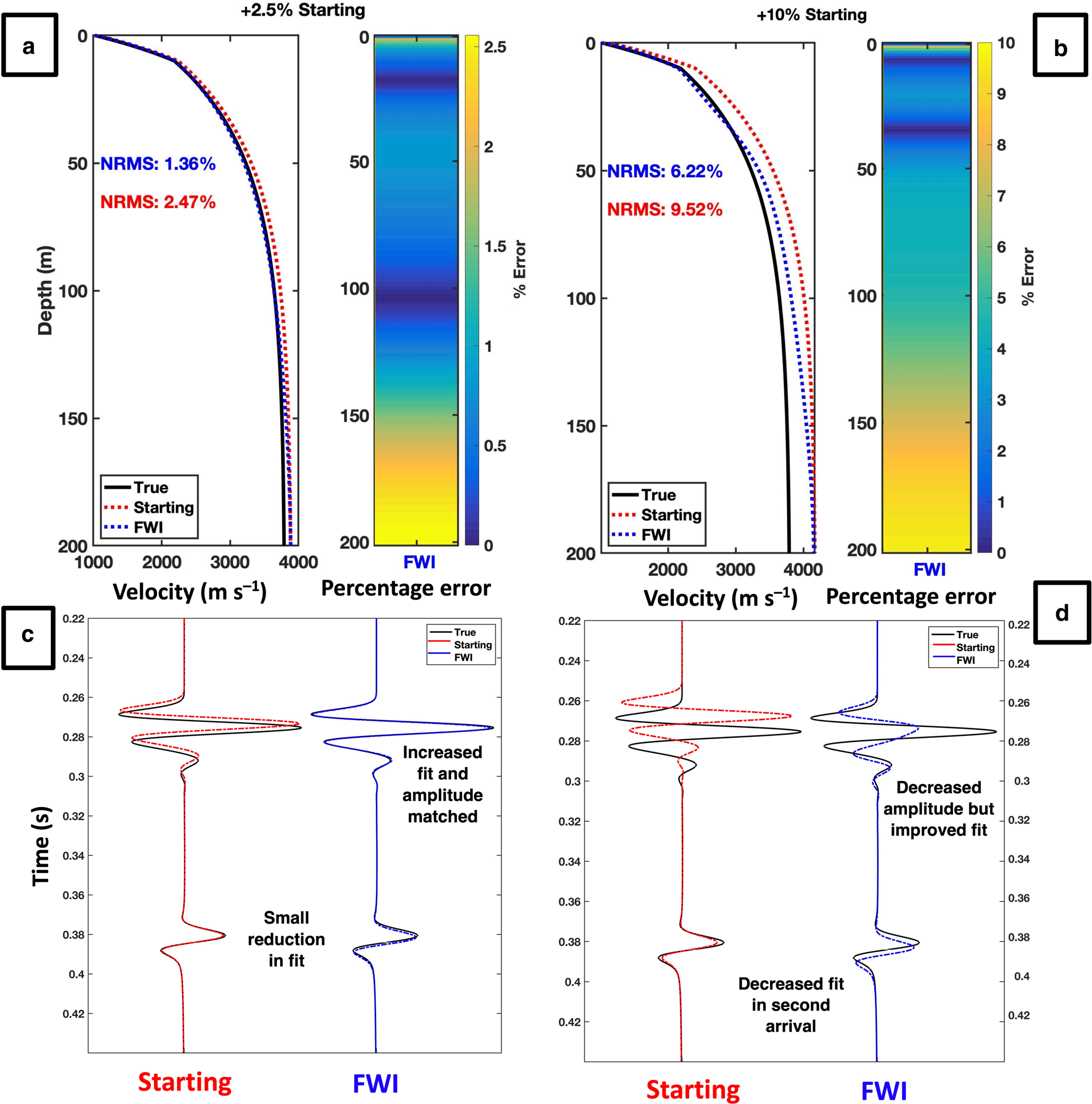
The observed (true), starting (predicted) and updated (FWI) data for (a) a 2.5% starting model and (b) a 10% starting model. The data updated by FWI for the 10% starting model show cycle skipping from an offset of 300 m. The data update from FWI for 2.5% model shows no cycle skipping, but from an offset of 800 m, the peaks in the data are not fully matched.

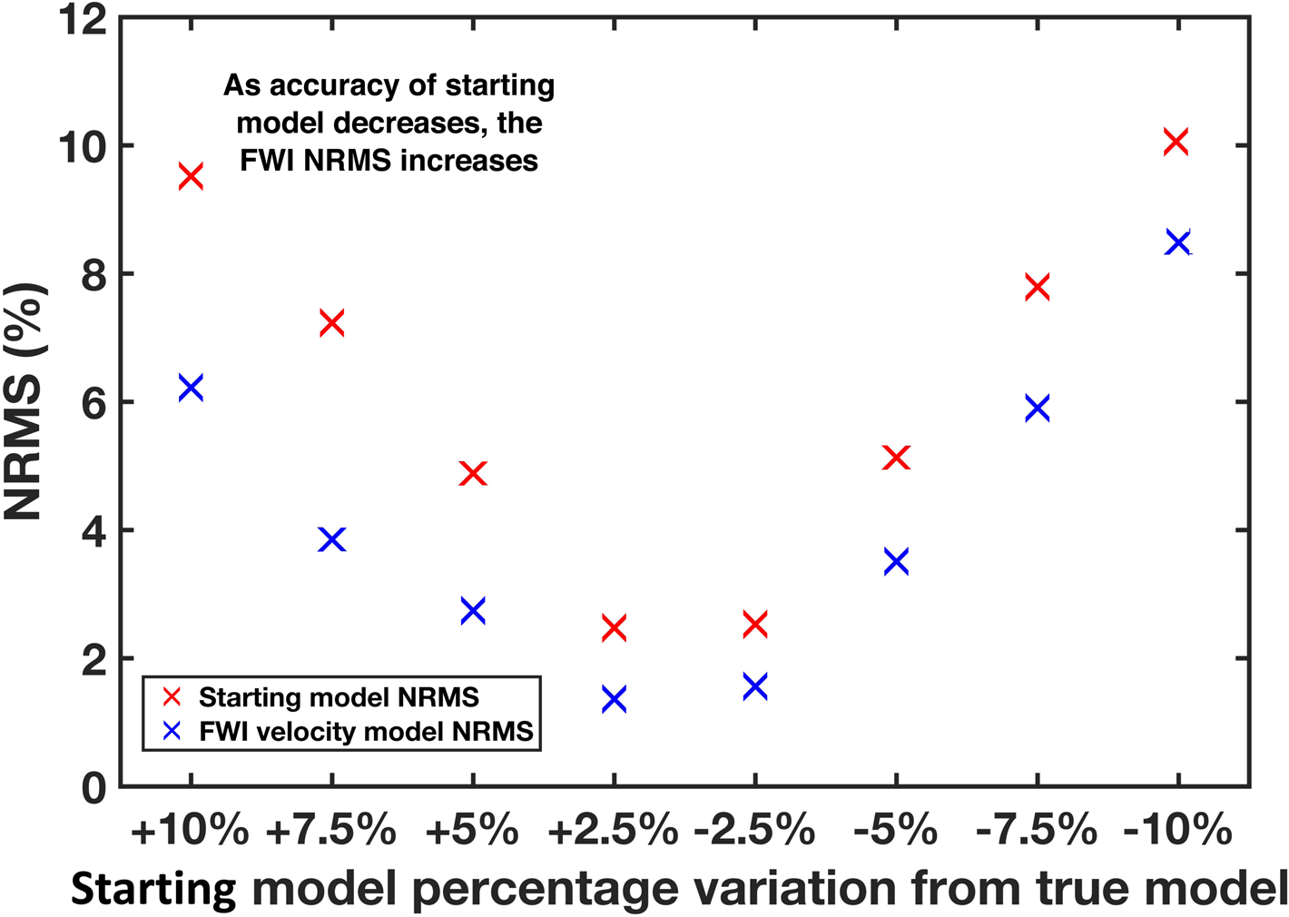
This perturbation analysis (summarized over Figs 6–8) shows that FWI can recover the true velocity model even with an incorrect starting model provided that the deviation does not exceed 2.5%. At larger deviations, the inversion becomes prone to cycle skipping in the far offset traces, and the depth to which a reliable inversion can be performed decreases. This is expected because the absolute mismatch between the starting and true velocity models is less in the shallow surface, where the velocity is smaller. Therefore, for the 60 Hz frequencies used in this study, FWI requires a starting model that is within 2.5% of the true velocity profile to provide reliable results.
(a) The NRMS update for eight starting model variations. As the perturbation to the starting model increases, the update by FWI is further away from the true model (i.e. a higher final NRMS). FWI is insensitive to whether a starting velocity model is under- or overestimated, producing similar results for both scenarios (Pavlopoulou and Jones, Reference Pavlopoulou and Jones2020).
4.3 Recovery of a firn profile from an incorrect snow accumulation regime
To determine whether FWI is able to resolve different accumulation regimes, we deliberately misrepresent the starting velocity model with substitute models corresponding to lower and higher accumulation.
When accumulation is overestimated in the starting model (Figs 9a, c), FWI improves the NRMS error by ~60%. The final NRMS mismatch is 3.5%, although velocities are overestimated in the depth range of 50–150 m, approaching 4000 m s−1. In this range, the starting velocity model is too far from the true model, causing cycle-skipping. However, when accumulation is underestimated in the starting model (Figs 9b, d), the improvement to the NRMS error is ~77% and the final NRMS mismatch is just 1.4%. These results suggest that FWI is largely robust to errors in an assumed accumulation model, although the starting velocity model should still be as accurate as possible to avoid cycle-skipping.
Velocity model outputs from FWI for a starting model that assumes (a) too high an accumulation, and (b) too low an accumulation compared to the true model. Figure (c) and (d) show the seismic data for trace 200, for a starting model from too high and low accumulation, respectively.

Combined, these results show the potential for stable FWI implementation for steady-state firn profiles. Although vulnerable to cycle-skipping errors, FWI can recover the seismic velocity structure of firn profiles when supplied with (i) a reasonable starting velocity model derived from initial HWI and (ii) constraint of the shallowest seismic velocity.
5. FWI detection of ice slabs
5.1 Thickness variations
In our experiment, the upper boundary of the ice slab is fixed at a depth of 30 m, and its thickness is extended from 5 to 80 m. Figure 10 shows selected examples of 5, 20, 40 and 80 m from this thickness range, and results are summarised in Figure 11.
Velocity model outputs from ice slabs of different thickness (a) 5 m, (d) 20 m, (g) 40 m and (j) 80 m. As ice slab thickness increases, the base of the ice slab propagates into firn with a greater compaction, and therefore seismic velocity. As such, the velocity anomaly between the firn and ice slab is smaller at greater depths.

The reduction in NRMS achieved by FWI. An ice slab of greater thickness has the largest starting NRMS error but can be corrected by FWI.

For any ice slab thickness exceeding the minimum wavelength of the seismic data (here, λ = 20 m) (Fig. 10d), FWI models show a distinct deviation towards increased velocity compared to the starting model. Thinner layers cause a perturbation to the FWI velocity model, which could be used to infer the presence of a slab, but they are unable to resolve its thickness or velocity. For the thinnest slab thickness of 5 m (Fig. 10a), FWI is not sensitive to the velocity anomaly and the NRMS error is similar in both cases. Comparison of similar tests between HWI and FWI by Pearce and others (Reference Pearce2023) highlights how the HWI is also not sensitive to velocity anomalies at the very near surface. For thicker ice slabs, particularly >2λ (40 m) (Fig. 10g), the velocity anomaly is recovered well by FWI: the maximum velocity in the slab is ~3800 m s−1. Furthermore, the velocity also correctly reduces in the undisturbed firn that underlies the slab.
As the ice slab thickness increases, the NRMS error between the true model and the starting model increases. An increase in slab thickness from 1 to 80 m results in an increase in NRMS reduction from ~5 to 60% (Fig. 11). In all cases, ice slabs thicker than 40 m (2λ) thick show a 50–60% decrease in NRMS while ice slabs thinner than 40 m only reduce NRMS by 5–27%.
5.2 Depth variations
For these experiments, the thickness of the ice slab is fixed at 30 m, and the depth of its upper boundary is varied from 5 to 80 m. Figure 12 shows selected examples of 5, 20 and 80 m from this depth range, and results are summarised in Figure 13.
Velocity models for ice slabs at varying depths (left), the associated percentage error for every 1 m depth sample (right) and the NRMS error for the whole velocity profile. (a) Ice slab is not detected. (d) Velocity inversion begins to be recovered. (g) Velocity inversion detectable and update is a clear divergence from background velocity trend. (j) The value of the objective function for each iteration. The greatest decrease in the OF comes in the lowest frequency. As ice slabs are located deeper in the firn, the velocity anomaly caused by their presence within the background firn compaction trend is proportionally smaller, resulting in a smaller objective function.

The reduction in NRMS achieved by FWI for models with increasing depth of the ice slab.

For ice slabs at a depth of 5 m (Fig. 12a), no significant improvement to the velocity model is achieved by FWI. For these data, FWI increases the overall velocity of the starting model from a depth of 5–60 m and does not recover the velocity inversion, instead introducing a localised velocity update where the ice slab is located. When the ice slab is located at depths of ≥20 m (Figs 12d, e), a localised update to the starting model is observed, and the velocity inflexion at the base of the ice slab is detected. The precision of the velocity inflexion marking the upper and lower interface of the slab increases with depth, given that the starting model becomes closer to the true model. This is consistent with the performance of the previous models, in which the resolution of thicker ice slabs was improved given the smaller deviation to the starting velocity model. Increasing the slab depth over the full range investigated, from 5 to 100 m, results in an increase in NRMS reduction from 13 to 51%.
Resolution limitations to detect ice slabs with FWI are based on the minimum wavelength of the seismic data. When ice slabs are present with a thickness similar to the wavelength (20 m), FWI begins to update the starting model at the depth of where the ice slab is located. As the thickness of the ice layer increases, FWI recovers the true velocity anomaly well, with 40 m (2λ) thick layers accurately predicting the expected 3800 m s−1. Layers thinner than the dominant wavelength are still detected by FWI, causing deviations to the recovered velocity model; however, FWI does not recover ice velocities correctly in such cases. Ice slabs located within a depth interval less than the minimum wavelength are recovered as a single ice slab, with increasing distance between the features resulting in improved characterisation of the two layers.
6. Discussion
6.1 Advantages of FWI over conventional inversion approaches
The firn layer is important to understand as it can provide insight into the accumulation history of a glacier and should influence the design and interpretation of geophysical surveys that aim to explore basal glacier properties. We show that acoustic FWI can be used to improve reconstruction of the seismic structure of firn, compared to conventional travel time tomography approaches. FWI can improve the recovery of the velocity structure of steady-state firn, leading to improved assessment of density and understanding of the accumulation regime. Furthermore, FWI yields accurate results even for poor starting models, provided that the deviation between the true and starting velocity models is small enough to avoid cycle skipping. We show that FWI can determine the depth and thickness of ice slabs located within the firn column, although the precise resolution and accuracy depends on the thickness and depth of the ice slab (improving with increasing depth and thickness).
Analysis of a range of synthetic firn structures, including steady- and non-steady-state accumulation, shows FWI can perform at least as well as HWI travel-time tomography approaches, but performs particularly well when a better estimate of the velocity in the upper 2 m is provided. This suggests that ground truth measurements of the very near surface velocity are required for this algorithm. When FWI is used with the HWI velocity model as a starting model, the improvements of the velocity model accuracy produced by FWI are small (with a maximum NRMS reduction of 0.5% to the starting velocity model). An advantage of FWI, however, is that it can overcome errors in an HWI-derived starting model given its iterative model update. At the very least, the FWI output will be no worse than that initially derived from HWI.
Booth and others (Reference Booth2013) compared ground-penetrating radar (GPR) with seismic refraction for reconstructing the thickness and density of glacier snow-cover. GPR was found to be more successful for accurately determining snow thickness, but seismic-derived velocities were more closely related to densities measured in a co-located snow pit. Although empirical relationships are still required to convert seismic velocity to density, FWI has shown that the velocity terms in such conversions can now be evaluated more reliably. Furthermore, with the extension of our acoustic FWI approach to an elastic inversion, it may be possible in the future to invert directly for firn density, thereby circumventing empirical approaches altogether.
6.2 Real-world applications of FWI methods
The presence of ice slabs influences meltwater drainage and runoff across glaciers and ice masses (MacFerrin and others, Reference MacFerrin2019). In the case of ice shelves, this decrease in permeability and increase in surface meltwater can lead to a reduction in ice shelf stability (Munneke and others, Reference Munneke, Ligtenberg, van den Broeke and Vaughan2014). This was observed on the Larsen B ice shelf, where firn compaction, meltwater ponding and hydrofracturing were strongly implicated in the ice shelf's rapid disintegration in 2002 (Scambos and others, Reference Scambos, Bohlander, Shuman and Skvarca2004). FWI analysis of seismic data obtained over this region could have provided insight into the internal structure of the ice shelf prior to its collapse and motivates the application of FWI to existing ice shelves of concerning stability such as Larsen C Ice Shelf (LCIS).
Hubbard and others (Reference Hubbard2016) imaged a 40 m-thick ice slab in a borehole located in Cabinet Inlet (in the upstream reaches of the northern sector of LCIS) and interpreted the ice as having formed from the accumulation of episodically refrozen surface meltwater ponds. Here the firn zone is 10°C warmer and 170 kg m–3 denser than undisturbed firn in the surrounding area. Regional geophysical surveys suggested that the ice slab is at least 16 km across and several kilometres long. While GPR surveys (Booth and others, Reference Booth2018) were able to constrain the layer's thickness and seismic velocity models (Kulessa and others, Reference Kulessa2015) were consistent with pure ice, neither method could establish both the full depth extent and velocity anomaly of the slab. FWI methods show promise for applications such as this, particularly given that the thickness of the slab exceeds more than twice the wavelength of the seismic data presented in Kulessa and others (Reference Kulessa2015).
The next steps for FWI in glaciology are to apply these synthetic-based observations to real data. Notable requirements observed from the synthetic studies are the use of very near offset receivers to record the reflection from the ice combined with long offset to record the deep refractions. A form of ground truth in the very near offset will aid to prevent cycle skipping, and improve the likelihood of a successful FWI. The seismic source should be as rich as possible in low frequencies, to facilitate the initiation of the inversion. Here, we invert up to a maximum frequency of 60 Hz, but 60 Hz is often at the lower end of the bandwidth of a typical glaciological seismic source wavelet (e.g. Peters and others, Reference Peters2008; Brisbourne and others, Reference Brisbourne, Kendall, Kufner, Hudson and Smith2021). As such, it is likely that some effort must be directed to producing a source wavelet that is richer in low-frequency content (e.g. using Vibroseis technology; Eisen and others, Reference Eisen2015).
7. Conclusion
It is important to be able to map firn structure and hydrology to understand process and to guide models of the stability of ice shelves, in particular the impact of impermeable ice slabs. Ice slabs can be detected and characterised by several geophysical methods, but FWI methods show potential for significant improvement over established methods. Using synthetic steady-state firn velocity profiles produced by the Herron and Langway densification model, we show FWI offers improved reconstructions over conventional approaches when the starting velocity model was a poor representation of the subsurface (as it commonly is). In non-steady-state cases featuring ice slabs, FWI improves the constraint of slab depth and thickness, which is currently impossible to do with established HWI approaches.
These synthetic analyses suggest that FWI should be considered in future seismic campaigns in glaciology, particularly over complex subsurface structure with minimal ground-truth control. The next steps for FWI in glaciology require the acquisition of FWI-compliant seismic data from real-world applications to validate our model approaches. Any location with ice slabs within the firn column would be appropriate, particularly at critical sites such as LCIS (e.g. for validation and the necessary shallow ground-truth constraint) makes it an attractive proposition for a test case.
Data
Synthetic firn seismic velocity profiles are available to download from the figshare repository, https://doi.org/10.6084/m9.figshare.20765350.v1 (Pearce, Reference Pearce2022).
Acknowledgements
This research was funded by the Natural Environment Research Council of the UK, under Industrial CASE Studentship NE/P009429/1 with CASE funding from ION-GXT. Additional support was obtained from The International Association of Mathematical Geoscientists. Roger Clark and Emma Smith are thanked for their constructive discussion and support with this research and manuscript. Comments from three anonymous reviewers greatly benefitted the preparation of the manuscript.


 Open access