


1. Introduction
Rising levels of income and wealth inequality in the United States and other developed economies since the 1980s have attracted renewed attention to the dynamics of wealth accumulation. Whether market economies display a tendency toward rising inequality remains an open question. There is evidence, however, that major economic dislocations such as the Great Depression and World War II – and the policies enacted during this period – temporarily reversed the trend toward increasing inequality. Piketty (Reference Piketty2014: 275) showed that, “it was the chaos of war, with its attendant economic and political shocks, that reduced inequality in the twentieth century…In the twentieth century it was war, and not harmonious democratic or economic rationality, that erased the past and enabled society to begin anew with a clean slate.” But there is relatively little evidence from earlier time periods that would contextualize these mid-twentieth century events.
In this paper we offer new evidence from an earlier period by examining patterns of wealth mobility in the United States over the Civil War decade. The U.S. federal censuses of 1860 and 1870 included questions about personal and real property wealth, allowing us to examine how the Civil War and the resulting emancipation of enslaved African Americans affected property ownership.Footnote 1
In addition to contributing to the larger literature on the dynamics of wealth inequality our analysis also contributes to an historical literature that has sought to trace the effects of emancipation on the southern elite. Among early analysts of the effects of emancipation, the prevailing argument was that emancipation had been accompanied by the displacement of the prewar elite (see, e.g., Hammond Reference Hammond1897). Reflective of this view, Buck (Reference Buck1937: 145) concluded that: “The small, rich landowning aristocracy in whose interest so much of Southern energy had been expended was deprived of its privileged position.” Yet, by the time Buck was writing a new view based on more quantitative evidence was beginning to emerge. Reflecting this new perspective, Shugg (Reference Shugg1937) argued that the plantation system was not destroyed by the war and that land ownership actually became more concentrated after the Civil War.
The most influential modern works on this subject are Jonathan Wiener’s (Reference Wiener1976, Reference Wiener1979) studies using census data for five Alabama counties. Relying on manuscript censuses from these counties, Wiener analyzed a sample of the 263 largest landholders in 1860, seeking to locate them in the 1870 census. He then compared their persistence rate over the 1860s with the persistence of a comparable group between 1850 and 1860. Finding that the rate of persistence in the 1860s (43 percent) was close to that of the 1850s (47 percent), he concluded that this supported Shugg’s argument that the wealthy planter elite had been successful in retaining their position despite the disruptions of the Civil War. Ransom and Sutch (Reference Ransom and Sutch1977) concurred with Wiener that the land ownership patterns were quite stable over the decade allowing the prewar elite to retain their political and social influence in the postwar South.Footnote 2
An important limitation of the studies by Wiener and other quantitative historians is their limited geographic scope. In the absence of comprehensive finding aids for the census, data could only be gathered on individuals who remained within a narrow geographic area. Thus, the fate of individuals who migrated out of the region of study could not be determined. Their departure might have reflected a response to downward mobility, but it was equally possible that they had moved in pursuit of new and more attractive opportunities elsewhere. As Massey (Reference Massey2016: 5) notes, matching individuals within restricted geographic areas “poses a serious threat to the representativeness of the matched sample.”
In the past decade, however, advances in electronic finding aids for historical censuses combined with online access to complete census manuscripts for the entire country, has eliminated these technical constraints and enabled a new generation of scholars to trace individuals regardless of geographic mobility. In a recent article, we analyzed the top 5 percent of wealth holders in the North and South found in the IPUMS 1 percent sample of the 1870 census, linking them backward to the 1860 census using Ancestry.com’s search function and then locating them in the 1860 wealth distribution (Dupont and Rosenbloom Reference Dupont and Rosenbloom2018). We found that while there was substantial persistence among the southern elite, the rate of downward (and upward) mobility was greater in the South than in the North. While 40 percent of the wealthiest northerners in 1870 had been in the top 5 percent in 1860, less than 28 percent of the richest southerners had been in the top 5 percent in 1860.
Using the complete-count digitized version of the 1860 census linked to the 1870, 1880 and 1900 censuses Ager et al. (Reference Ager, Boustan and Eriksson2019) were able to trace the fortunes of southern household heads and their sons over a substantially longer period. Consistent with Dupont and Rosenbloom (Reference Dupont and Rosenbloom2018) they found that southern slaveholders experienced larger drops in wealth than other household heads. However, they reported that by 1880 the sons of southern slaveholders had rebounded, achieving a status comparable to that of their fathers before the Civil War. Because questions about wealth were included only in the 1850, 1860 and 1870 censuses, however, comparisons beyond this period must be based on the inferred status of different occupations rather than on a direct comparison of wealth.
In this paper we offer an additional perspective on the effects of the events of the 1860s through a comparison of a random sample of household heads in all regions of the country drawn from the one percent sample of the 1860 census and linked forward to the 1870 censuses. While the Ager et al. (Reference Ager, Boustan and Eriksson2019) analysis focused on the differential effects of slave ownership on the fortunes of southerners, we explicitly consider inter-regional differences in wealth mobility. And in contrast to our earlier work, by using a random sample of prewar wealth holders we are better able to analyze the factors that were associated with upward and downward mobility over the decade. With this new sample we find that overall wealth persistence was remarkably similar across regions, even though most of the effects of the Civil War were concentrated in the South. Nonetheless, we do find some evidence that emancipation produced greater wealth mobility in the South. Specifically, we show that the correlation of personal property ownership (which included slave wealth in 1860) between 1860 and 1870 was lower in the South than in the North, but that the magnitude of this difference was too small (and the overall volatility of wealth too great in both regions) to affect the behavior of total wealth in the decade.
Inequality had been rising since the start of the century and was high everywhere by 1860, but the southern slave economy had the most unequal distribution of wealth (Lindert and Williamson Reference Lindert and Williamson2016). The Gini coefficient on total property wealth was 0.82 in the south prior to the war compared to 0.75 in the north.Footnote 3 Roughly half of Southern wealth was in the form of enslaved persons, yet ownership of slaves was itself deeply unequal. Soltow (Reference Soltow1975) found that only 21 percent of white Southerners owned slaves while about 0.5 percent owned more than 50 slaves. The war and slave emancipation of course dramatically impacted the southern economy – median wealth in our sample in 1870 was only about three-quarters of its 1860 level. And overall inequality fell in the south as well – the Gini coefficient on total property wealth fell to 0.79 in 1870 as the share of wealth held by the top 10 percent in our sample fell from 71.7 to 66.8 percent over that decade. These changes in regional wealth holding and its distribution are reflected in Figures 1A and B, which compares total property holding at several different points in the wealth distribution across Northern and Southern states in 1860 and 1870.
A. 1860 Wealth Distribution and B. 1870 Wealth Distribution.

The powerful redistributive effects of the war and emancipation were enough to halt what would likely have been a continuation of the sustained increase in inequality that occurred in the first half of the 19th century, so it is important to carefully document the changes that occurred in this decade. We turn to our analysis of these events in Sections 3 and 4 but first describe the dataset that we constructed.
2. Data
In the absence of unique and reliable identifying information that would allow individuals to be unambiguously linked between different data sources, such as successive censuses, researchers seeking to create linked data must draw inferences about whether observations in different sources are truly the same person based on commonly available and time invariant information such as name, birth year, and birth place. In doing so, they must contend with the fact that names may change over time because Census enumerators may have misspelled them, the household respondent may have reported them incorrectly, or an individual may have changed her/his name. Age and birth year may differ across sources due to a tendency of people to round age to the nearest multiple of 5 (“age heaping”). Similarly, respondents may provide somewhat different information about birthplace at different times. Digitization of the original handwritten records can introduce further errors, when the original information is difficult to read or is transcribed incorrectly (Bailey et al. Reference Bailey, Cole, Henderson and Massey2020: 1000–1003; Abramitzky et al. Reference Abramitzky, Boustan, Eriksson, Feigenbaum and Pérez2019: 2–3). Finally, mortality and emigration mean that some individuals are not available to be enumerated in subsequent data sets.
For these reasons, constructing a linked data set requires a series of subjective judgments about whether an individual located in one source is in fact the same person as the one found in another. Among the most important questions to consider are whether the names are sufficiently similar and whether the reported age is close to what it should be. As the criteria for accepting non-exact matches are loosened more matches may be made, increasing the size of the linked sample. But at the same time, this increases the possibility of incorrect linkages (Type I errors), in which two different people are assumed to be the same person, which introduces spurious matches. While stricter linkage criteria reduce the number of incorrect linkages, they increase the likelihood of rejecting correct linkages (Type II errors). Both Type I and Type II errors are problematic, though for different reasons. Including incorrect linkages introduces noise in the data with a resultant attenuation of estimated parameters. Rejecting true links reduces sample size and hence statistical precision. Moreover, if the rejected links are systematically selected, these Type II errors can introduce sample selection effects into the resulting data.
As access to machine readable full count census data has become more widespread in the last few years, scholars have begun to automate the implementation of linkage algorithms, making possible the creation of much larger linked data sets than were previously available and enabling comparisons of the effects of different linkage algorithms on which observations are linked. Bailey et al. (Reference Bailey, Cole, Henderson and Massey2020) provide an excellent overview of the different approaches to record linkage that have been adopted by researchers and evaluate how well each performs on several data sets for which the ground truth is known with a high degree of certainty. Their comparisons imply that the automated linkage methods that have been used in several recent studies (Abramitzky et al. Reference Abramitzky, Boustan and Eriksson2014; Feigenbaum Reference Feigenbaum2016; Nix and Qian Reference Nix and Qian2015) are prone to accepting incorrect links in up to 37 percent of cases. Interestingly, many of these methods also increase the number of incorrectly rejected links. The reason for both seems to derive from phonetic name processing and other approaches to inexact name matching. Because these approaches reduce spelling variations, they result in more potential matches which increases the chance of incorrect matches. At the same time, the standardization of names increases the likelihood of rejecting a true match because it increases the likelihood of multiple matches that cannot be disambiguated.
Abramitzky et al. (Reference Abramitzky, Boustan, Eriksson, Feigenbaum and Pérez2019) have recently revisited the performance of automated linkage algorithms and come to a more optimistic conclusion than Bailey et al. (Reference Bailey, Cole, Henderson and Massey2020) concerning their performance. Overall, they conclude that different automated algorithms trace out a frontier of trade-offs between Type I and Type II errors, and that hand methods also typically lie along this same frontier. The obvious advantage of automated methods is their ability to create much larger data sets, and therefore enable more precise estimation of effects. Importantly, Abramitzky et al. (Reference Abramitzky, Boustan, Eriksson, Feigenbaum and Pérez2019) argue that the choice of method is likely to be dictated by the use to which the linked data are to be put, and that rather than focusing on one “best” linkage approach it is desirable to assess how robust conclusions are to the use of different algorithms to construct the linked data.
When this project originated, hand linking records was the only way to explore this topic, so our main analysis is based on the hand linkage procedures we describe below. However, the Census Linkage Project (https://censuslinkingproject.org/) recently released crosswalk files that make it possible to link individuals across all publicly available U.S. censuses, and IPUMS has made full count census data available for download. While we have not had the opportunity to subject these data to the same level of scrutiny as our hand-linked sample, we have reproduced the analysis reported here using samples created using these sources and include the results of these analyses in the appendix. As we discuss below and in the appendix, the primary conclusions of our analysis are robust to the use of these alternative samples.
For this paper we have hand-collected a set of 1,679 observations of household heads linked between the 1860 and 1870 federal censuses. To obtain these data we began by drawing a random sample of 8,400 household heads from the one percent sample of the 1860 federal population census available through IPUMS (Ruggles et al. Reference Ruggles, Flood, Goeken, Grover, Meyer, Pacas and Sobek2020, downloaded 1/3/2018). To ensure reasonable geographic representation we stratified our initial sample by census regions: we selected 4,000 observations each from the North and South, and 400 observations from the western states. Footnote 4 After dropping individuals younger than 15 and older than 75 in 1860, the sample is reduced to 8,313 observations.
A team of three undergraduate research assistants then searched for each individual using Ancestry.com’s search algorithm based on first and last name, birth year, birth location, and gender. Ancestry’s search algorithm uses Soundex to produce search results for exact and similar name matches. Our research assistants reviewed the search results. If there was an exact and unique match, they were instructed to accept it and record data from the 1870 census manuscript. If there was no exact match, they reviewed the search results for names that appeared acceptably similar and had a birth year within 2 years of that inferred from the 1860 census. If multiple matches met these criteria, they were instructed to consider place of birth to break these “ties.” In cases where it was not possible to uniquely resolve the match, they were instructed to treat the case as an unsuccessful link. Footnote 5
Census officials at the time, and some later scholars have expressed concern about the high rate of under enumeration in the 1870 census, which could depress the rate of successful linkage. However, according to Hacker et al. (Reference Hacker, Ruggles, Foroughi and Sargent1999: 129), “the undercount estimate given in the 1890 census report was greatly exaggerated as a result of a failure to account for the magnitude of the negative demographic shock caused by the Civil War.” They point out that to arrive at the estimate of a 1.2 million person undercount, the 1890 investigators had assumed that the South experienced steady population growth between 1860 and 1880. Recent studies, however, have suggested that the Civil War substantially slowed population growth in the 1860s relative to the pace in the 1870s. Adopting a more realistic set of assumptions about the rate of population increase in the 1860s implies an undercount of about 6.6 percent, not significantly different from nonresponse rates in modern survey data (Hacker, Reference Hacker2013). On this basis Hacker et al, argued that the “under enumeration of southern whites and blacks in 1870 was far lower than 1890 investigators estimated. [The 1870 census] will not pose a significant problem for most analyses.” Similarly, Sutch (Reference Sutch2017: 605) argued that “a careful analysis based on the IPUMS data files for a sequence of censuses suggest that the undercount in 1870 was not nearly as great as some nineteenth-century observers had claimed.” A related concern is that measures of wealth concentration may be distorted by under-reporting which could bias measures of the concentration of wealth. After careful consideration, however, Sutch (Reference Sutch2017: 606) concluded that “Because many of those excluded were young children and the very poorest of adults the likelihood of a serious bias is reduced. If anything, the rich with their substantial dwelling units and their social prominence are likely to have been relatively well counted.”
Our linkage rate of 1,679/8,313 (20.2 percent) is roughly consistent with that of other researchers linking records forward from one census to a later one (Bailey et al. Reference Bailey, Cole, Henderson and Massey2020). Because marital status and children are endogenous and may be correlated with other characteristics of interest, we did not use information about other household members as a criterion to select links. However, comparing data on spouses and children, when present, offers an independent assessment of the quality of the linked data. In 922 (about 55 percent) of the linked observations we are able to confirm that another household member present in 1860 was also present in the 1870 census records for the household. Of the 8,400 household heads in our original random sample, 7,565 (90 percent) had a spouse or child in their household in 1860. The share of successfully linked observations with a spouse or child present was even higher (94 percent). In addition to the usual obstacles that reduce forward match rates (misspelled names and name changes, for example), children form independent households and parents may separate or remarry over time. Considering these challenges, the fact that we can confirm over half our links through the presence of other family members in both census reports provides independent confirmation of the quality of our linkage procedure.Footnote 6
Table 1 summarizes the results of our linkage effort, comparing a variety of demographic characteristics between the linked (column 2) and unlinked (column 1) observations. We also report the same summary statistics for those “high quality” links (column 3) in which another household member can be linked across the two census years. The fourth and fifth columns report, respectively, the t-statistics for the difference in means between the linked and unlinked observations and the p-value of this test statistic.
Comparison of linked and unlinked observations

Notes and Sources: All values are as of 1860. See text for description of linkage procedures.
There are a number of systematic differences between the linked and unlinked observations. Compared to the unlinked, our linked sample is about 15 months older, was more likely to report non-zero wealth in 1860 was less likely to be foreign born, less likely to be nonwhite, and less likely to be living in an urban area. The average wealth of the linked sample is also somewhat higher, although this difference is not statistically significant. In addition, it is apparent that we were more successful in linking individuals residing in the North in 1860 than those living in the South or West. Given the more pronounced effects of the Civil War on the southern economy and the greater geographic mobility of individuals in the West it is perhaps not surprising that this is the case. For the most part the occupational distribution of the linked and unlinked samples is quite similar, although farmers are overrepresented in the linked sample and service workers, laborers and those in the non-occupational category are underrepresented. We observe similar patterns of selectivity among the linked observations produced by the Census Linkage Project matrices using the Abramitzky et al. (Reference Abramitzky, Boustan, Eriksson, Feigenbaum and Pérez2019) algorithms (see Appendix Table A1 in Supplementary material). Because of the stratification of our hand-linked sample, it includes a higher proportion of southern residents than are produced by the automated linkage method applied to the whole population, which affects several other characteristics as well. Nonetheless in the automated linkage case we find that successfully linked observations are older, wealthier, less likely to be foreign born and more likely to be northern residents.
3. Wealth mobility
One way to describe wealth mobility over the 1860s is to look at individual movement within the wealth distribution in the two years; that is to look at relative wealth mobility. This is the approach we took in our earlier analysis (2018). Before considering the data, however, it is important to note that emancipation presents an inherent challenge to these comparisons. In 1860, enslaved persons were not enumerated in the population census. In 1870, however, the formerly enslaved were included in the population count, which added to the size of the overall population, especially in the South. Because the formerly enslaved were mostly propertyless, the added observations were concentrated in the bottom tail of the distribution. The larger population expands the size of each percentile category, which should lower the threshold wealth dividing each group relative to those calculated using only those enumerated in 1860. Other things equal, comparisons that use the entire population in 1870 would tend to bias the results toward upward mobility among the 1860 free population. Ideally, we would like to be able to track movements in the wealth distribution within a consistently defined population. The best we can do in this case, however, is to locate individuals relative to the distribution of wealth among white household heads in both 1860 and 1870.
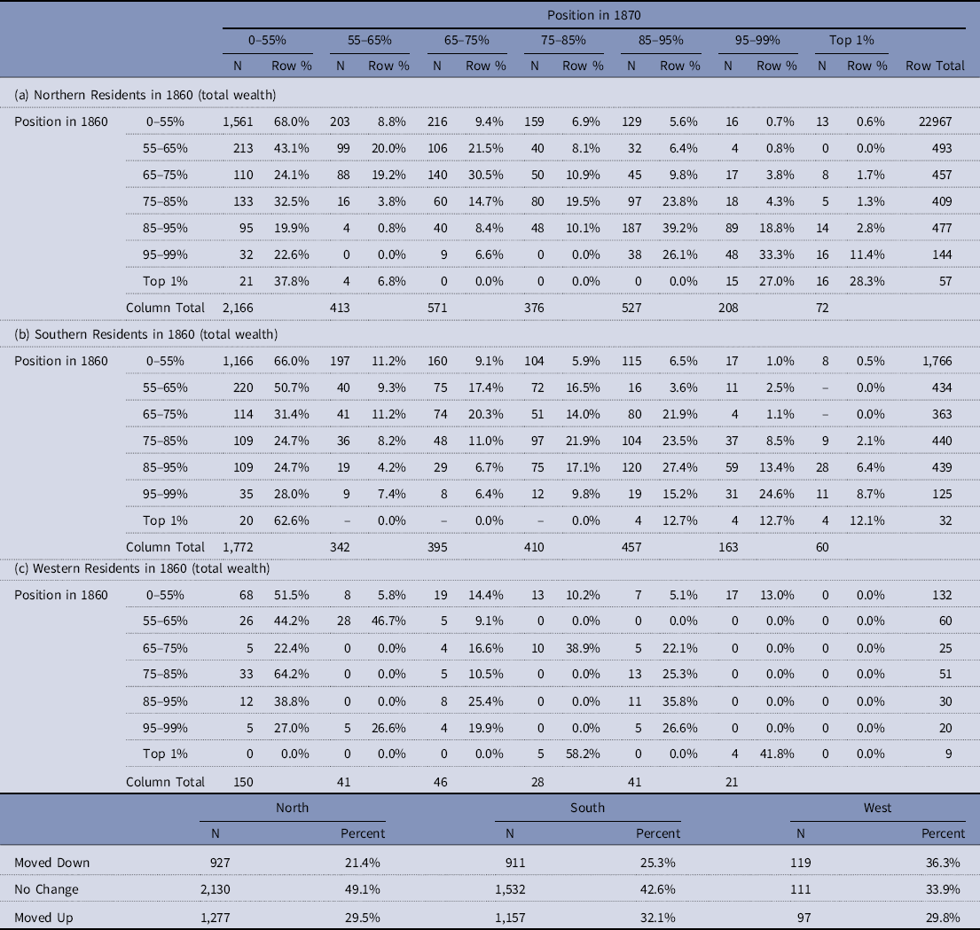
In Table 2 we compare individuals’ locations in the distribution of total property ownership between 1860 and 1870 based on their 1860 region of residence. To do this we first use data on all white household heads in the 1 percent samples of the 1860 and 1870 censuses to characterize the distribution of wealth in each region in each year and use this information to locate individuals in our linked sample within the regional wealth distribution in each year. We aggregate the bottom 55 percent of wealth holders because most of this group reported zero wealth holding and it is not possible to discern movement up or down within this group.
Total wealth rank transitions, 1860–1870, by Region (using the white population) – weighted
To address the sample selectivity introduced by the linkage process, we reweighted the wealth mobility calculations to reflect different probabilities of linkage, by breaking the sample of 8,400 individuals into 24 cells defined by 10-year age groupings (15–25 years, 25–35 years, etc.), nativity, and an indicator for urban residence. We then calculated the probability of linkage within each of these cells, and reweighted observations using the inverse of the linkage probabilities.Footnote 7
In Table 2, the rows of each panel count individuals based on their position in the 1860 wealth distribution, while the columns count individuals based on their position in the 1870 wealth distribution. The cells along the diagonal of the table represent individuals who neither moved up nor down. Cells to the right of the diagonal represent individuals who moved up in the wealth distribution, while cells to the left represent individuals whose wealth status declined over the decade. Panel (a) reports mobility for residents of the Northern states in 1860, while panels (b) and (c) show similar data for residents of Southern and Western states, respectively.
In all three regions there is a considerable degree of movement, both up and down the wealth distribution over the decade. In the North, for example, of 2,297 household heads in the bottom 55 percent of the wealth distribution in 1860, 1,561 (68 percent) remained in this category in 1870, but 203 had moved into the 55th-65th percentile, while 216 had moved into the next tier (65th-75th percentile), and 316 had moved up even further, with 29 reaching the top 5 percent of 1870 wealth holders. A very similar movement is apparent in the South where 66 percent of those in the bottom tier of the wealth distribution remained in that category in 1870, but 34 percent had moved up.
One way to summarize the overall pattern of movement within regions is to count the numbers of those who moved down the distribution, remained in the same relative position or moved up. We report these figures at the bottom of the panels in Tables 2, 3 and 4. Since wealth accumulates with age, we would expect, other things equal, that household heads in 1860 would move up the wealth distribution over the succeeding decade as they aged and accumulated wealth. We see some evidence of this – more northern and southern heads of household moved to higher wealth categories than moved to lower ones – but there is significant stability within the wealth distribution in both regions. A plurality of households in the north and the south were in the same wealth category in 1870 as they were in 1860 whether we measure total wealth or its components. And we see a fairly large percentage of households that moved down the wealth distribution, sometimes considerably. The west is somewhat different, with the largest percentage of those households moving down the wealth distribution, but the small sample size for this region should lead us to interpret those results with caution.
Transitions among real wealth percentiles, 1860–70 (using white population distribution)

Transitions among personal wealth percentiles, 1860–70 (using white population distribution)

Using the automated linkage data (Appendix Table A2 in Supplementary material), we find a higher level of upward mobility than in our hand-linked sample. For individuals in all 1860 regions of residence, movement up the wealth distribution represents the plurality of observations, while the number moving down the wealth distribution is lower. There is still considerable persistence in wealth holding, however, with 39 percent of northern residents and 38 percent of southern residents remaining in the same wealth percentile range across censuses. At the same time, the automated linkage data confirm the conclusion that patterns of mobility were quite similar in the North and South.
Because individuals reported personal and real estate wealth separately, we can also examine the evolution of wealth holding in these separate categories. Personal property includes “bonds, stocks, mortgages, notes, livestock, plate, jewels, or furniture, but exclusive of wearing apparel.” Slaves were included in the 1860 census as part of personal property. Real property reflects the full market value of real estate without deduction for encumbrances, although Steckel (Reference Steckel1990) pointed out that because mortgages in this period were of short duration and required large down payments, these data approximate net worth in real estate. Tables 3 and 4 report wealth transition tables for each of these wealth categories, respectively. There is greater stability in the wealth distribution when we look at real property wealth as compared to personal wealth. For real property wealth, the percentage of households that did not change positions in the wealth distribution were 47 and 45 percent for the north and south, respectively. But for personal wealth, those figures drop to 42 and 38 percent, respectively.
In our earlier work (2018), we found that there was more turnover among top wealth holders in the south. Our results here similarly show that the top wealth holders in the north were more likely to be non-movers in the wealth distribution; for example, 42 percent of northerners who were in the 85–95th percentile of the total wealth distribution in 1860 were in that same category in 1870 but only 25.5 percent of southerners were. This same pattern holds throughout the top end of the total wealth distribution. Most of these north-south differences are driven by the personal property component of total wealth, which is not surprising given that the 1860 personal property for southerners included slaves. Footnote 8
The evidence presented in Tables 2, 3 and 4 indicates that broad patterns of wealth mobility in the North and South were similar over the 1860s, although there are noticeable differences at the top end of the wealth distribution, mostly driven by differences in the personal wealth category. There is also some evidence that wealth mobility in the more sparsely settled western parts of the country behaved differently, but because of the relatively small size of our linked sample from this region it is hard to draw firm conclusions about this.
4. The determinants of 1870 individual wealth holding
Transition tables of the sort reported so far illuminate patterns of relative movement within the wealth distribution. But we can also use our data to examine changes in absolute levels of wealth holding at the individual level. In this section of the paper, we take advantage of the full range of individual data available to more closely examine factors that influenced individual wealth holding at the end of the decade. In Table 5 we report results of regressing log wealth in 1870 on a quadratic function of age, log wealth in 1860, and indicators for race, nativity, and whether the individual is living in his or her state of birth in 1860.Footnote 9 To address the fact that many individuals report no wealth in one or both years we add $1 to reported wealth for all individuals. In 1870, census enumerators were instructed only to record personal property wealth for values of $100 or greater, so there is an understatement of property wealth for the poorer households. But since there was no such restriction in 1860, Rosenbloom and Stutes (Reference Rosenbloom, Stutes and Rosenbloom2008) argued that the 1860 wealth levels could reasonably be used to draw inferences about the 1870 data. They found that among the household heads with less than $100 in personal property wealth in 1860, two-thirds reported zero values. Given the relatively small number of households with nonzero personal property wealth of less than $100, the impact of this $100 lower limit in the 1870 data is likely to be minimal.
Tobit regressions

Notes: The excluded region is North. Estimated with robust standard errors. T-statistics in parentheses. *p < 0.05. **p < 0.01. ***p < 0.001.
About 24 percent of those in our dataset reported $0 in total property wealth in 1870 so our estimation strategy relies on a Tobit regression of wealth on a variety of controls. As we report in Table 5, we estimated three separate sets of regressions. The first three columns in Table 5 report the results of Tobit regressions for total wealth, the next three show personal property, and the final three show real property. These coefficients can be interpreted as the marginal effects of the various regressors on the natural log of wealth in 1870 for our full sample. Given the mass of observations at zero, we also estimated these marginal effects conditional on having positive reported wealth levels in 1870. These results are summarized in Table 6.
Marginal effects of key variables of interest in 1870 wealth

Note: The excluded region is North. T-statistics in parentheses. *p < 0.05. **p < 0.01. ***p < 0.001.
We find several economically and statistically significant determinants of wealth levels in 1870. As might be anticipated, wealth follows an inverted U-shape with respect to age. The average age (in 1860) for southerners in our sample is 41.8 years while northern residents were slightly older at 42.3 years. Using our preferred specification of the Tobit regressions (Models 2, 5, and 8), the coefficients on age and age-squared imply that real property wealth in 1870 peaked at 56 (46 in 1860); personal property wealth peaked at 47.5 (37.5 in 1860) and total wealth peaked at 51 (41 in 1860).
Median wealth levels fell dramatically in the south because of the Civil War. In 1860, median total property wealth in our sample was $1,153 but had fallen by about one quarter (to $880) in 1870. As a result of the rapid price inflation in the south, real wealth levels clearly fell even further. Between 1860 and 1870, consumer prices rose by about 57 percent, according to both the BLS-based and David-Solar-based indexes (Lindert and Sutch Reference Lindert, Sutch, Carter, Gartner, Haines, Olmstead, Sutch and Wright2016, HSUS Cc1-Cc2). Given the rapid inflation during this period, Lerner (Reference Lerner1955: 33) estimated that “real wages in the Confederacy had declined to well under 40 percent of their prewar level by March, 1865.” As expected, since much of this decline in wealth is attributable to emancipation, the decline in total property wealth was driven primarily by reduced personal property wealth. The impacts of the wealth shock caused by emancipation are evident in the coefficients on the regional indicator variables in our Tobit regressions. The coefficients imply that, other things equal, individuals living in the South in 1860 had lower levels of wealth in 1870 than comparable individuals living in the North.
Only about 15 percent of our sample reported having been born outside the United States, but those people tended to have lower wealth levels in 1870. Being born outside the U.S. has negative and relatively large effects on 1870 wealth levels, although these effects are only statistically significant in the case of personal property. We estimate similar effects for those living outside of their state of birth. On average, those who lived in their birth state in 1860 had higher wealth in 1870 than those who were residing outside their birth state, but this difference is largely driven by some extremely high wealth levels for a few individuals in the former group. In any case, none of the coefficients on this indicator is statistically significant.
For the sake of brevity, Table 5 does not report all of the separate occupational categories, but the first two sets of results for each of our wealth measures include controls for occupation. The results are consistent with what we might expect, implying higher 1870 wealth levels for farmers, managers and proprietors than for laborers and service workers. For the most part occupational effects are not statistically significant, but service workers in 1860, the unemployed and those giving other non-occupational responses did have significantly lower wealth in 1870. Footnote 10
Of primary interest in these regressions is the coefficient on 1860 wealth, which measures the elasticity of 1870 wealth with respect to wealth 10 years earlier. The larger this coefficient the more persistent wealth holding was across the decade. For each category of wealth, we begin by imposing a constant elasticity across regions, and then add an interaction term with indicator variable for each region allowing it to differ by region. The cross-decade wealth elasticity is greatest, indicating the most persistence, for real estate wealth, and lowest for personal wealth. Total wealth, which aggregates these two categories, lies somewhere in between. It is worth noting that none of these elasticities appears to be very high in absolute terms, particularly when we look at the elasticities conditional on having positive 1870 wealth levels, which we report in Table 6. Put differently there was a considerable degree of unpredictability in who was found higher up the wealth distribution in 1870. The low cross-decade correlation of wealth in the 1860s is consistent with Ward’s (Reference Ward2020) finding of relatively low correlations between occupational status measures for individuals observed across decades at the beginning of the twentieth century.
If the effects of the Civil War and emancipation reduced wealth persistence in the south relative to other regions, we would expect the wealth elasticity measure would be smaller in this region. We find some limited evidence that the estimated wealth elasticity is lower for 1860 residents of the south, although these effects are imprecisely measured, suggesting that despite the effects of emancipation on overall wealth holding in the region, the elimination of slave wealth did not introduce greater wealth mobility in comparison to the North. For residents of the western states, we do find a negative and statistically significant effect on wealth elasticity, consistent with our earlier finding of greater downward mobility for this group.
Results using the much larger automated linkage samples (Appendix Tables A5 and A6 in Supplementary material) are qualitatively quite similar to those we report here. With the larger samples we do find a somewhat higher own-wealth elasticity for all categories of wealth than in our hand-linked sample. But importantly there is no evidence that own-wealth elasticity varied significantly across regions. The coefficients on the region-wealth interaction variables are statistically significant and indicate that the elasticity was lower in the South than the North, but the size of these differences is so small as to be economically inconsequential.
The estimates in Table 5 impose a constant elasticity of 1870 wealth with respect to 1860 wealth. Using quantile regression we can however examine how the effects of 1860 wealth varied at different points in the 1870 wealth distribution. Footnote 11 In Table 7 we report the parameters of quantile regressions estimated at the 55th, 75th, and 90th percentiles of the 1870 wealth distribution, pooling observations across the different regions, while allowing for regional differences in the level of wealth. All of the regressions included controls for 1860 occupation, which are suppressed to simplify the presentation.
Determinants of 1870 wealth by wealth quantile

Notes: T-statistics in parentheses. *p < 0.05. **p < 0.01. ***p < 0.001.
Bootstrapped standard errors using 300 repetitions. The excluded region is North and all estimates include a full set of controls for occupational categories.
The first three columns of Table 7 report coefficient estimates for total property ownership, columns 4–6 report the estimates for real property, and columns 7–9 report the estimates for personal property. We find that the elasticity of 1870 wealth with respect to 1860 wealth was declining across wealth percentiles for each of these wealth measures, but that this pattern was much more pronounced for real property than for personal property. The declining coefficients on 1860 wealth as we move higher in the 1870 wealth distribution suggests that at higher points in the 1870 wealth distribution other unmeasured effects (chance) were more important than past wealth accumulation. Using the automated linkage samples (Appendix Table A7 in Supplementary material) we again find some changes in the magnitude of point estimates, but the conclusion that the own-wealth elasticity is declining as we move to higher points in the 1870 wealth distribution is strongly confirmed.
One of the central questions we posed at the outset of this article is whether the effects of emancipation and the Civil War caused wealth dynamics in the South to differ substantially from those in the North. In the Tobit regressions reported in Table 5 we found that regional effects on own-wealth elasticity were statistically insignificant. To assess regional variation at different points in the distribution we have re-estimated the models reported in Table 7 separately for the North and South. Table 8 reports separately the regional own-wealth elasticities for each type of wealth at the same three points in the 1870 wealth distribution as shown in Table 7. At the 55th percentile of the distribution, the own-wealth elasticity in the North appears to be considerably higher than it was in the South. However, as we move across the table to higher 1870 wealth percentiles the elasticities appear converge across regions. Moreover, there is a pronounced decline in elasticities in each region as we move higher in the 1870 wealth distribution. The conclusion is that while low wealth in 1860 helps to predict persistence at the lower rungs of the wealth distribution in 1870, movement into the higher rungs of the wealth distribution depended considerably more on chance events than on past wealth accumulation, and that this was true regardless of region of residence in 1860. Once again, the key points that we have emphasized based on the hand-linked data are confirmed with the machine-linked sample (Appendix Table A8 in Supplementary material). In particular, the pattern of declining own-wealth elasticities as we move to higher points in the 1870 wealth distribution is strongly confirmed in the larger samples, although point estimate magnitudes differ.
Regional quantile estimates of 1870 wealth elasticity

Notes: 872 observations for the North and 752 for the South. All regressions included a full set of controls for individual characteristics. T-statistics in parentheses. *p < 0.05. **p < 0.01. ***p < 0.001.
5. Conclusion
Ending slavery resulted in an historically unprecedented transfer of wealth from slave owners to the formerly enslaved. The war itself devastated large areas of the southern United States, and reconstruction resulted in significant political upheaval within the states of the Confederacy. Not surprisingly, historians have long been interested in how these multiple shocks affected southern society and southern elites. Recent interest among economists in issues of inequality and the dynamics of wealth distribution offer another reason for studying this episode.
Several recent studies have begun to exploit the ability to link data for individuals across multiple censuses to shed light on the evolution of individual fortunes. In this paper we offer additional evidence from a hand-linked sample of 1,679 household heads followed between the 1860 and 1870 censuses. Several important insights follow from our analysis. First, we find little difference in relative wealth mobility patterns between northern and southern residents in 1860. That is those at the top of the southern wealth distribution were just as likely to remain at the top in 1870 as was the case for northern residents. In 1860 western states were still relatively sparsely settled, and our sample for this region is small. Nonetheless, our data suggest that fortunes in this region were more dynamic, and that downward mobility was much more likely for residents in this region. Presumably, spaces at the top were filled by new residents moving into the region.
Second, we are able to examine in some detail the determinants of individual wealth holding in 1870 as a function of exogenous personal characteristics determined at the beginning of the decade of the 1860s. Consistent with the expected effects of emancipation, war and political turmoil, we find that after holding 1860 wealth and other characteristics constant southern residents had substantially (35 to 50 percent) less wealth in 1870 than did their counterparts in the North. We also find some support for the conclusion that the events of the 1860s created more mobility among southern wealth holders than in among those in the north. When we allow the elasticity of 1870 wealth with respect to 1860 wealth to vary by region of residence in 1860, our estimates imply that the effects of 1860 wealth were weaker for southern residents than for northern ones. Equally striking, however, is the low predictive value of 1860 wealth in determining 1870 wealth holding in all regions. The elasticities of 1870 wealth with respect to 1860 wealth that we obtain are comparable in magnitude to more contemporary estimates of intergenerational wealth or income elasticities. Thus, the relative similarity of wealth dynamics in southern and northern states in the 1860s is partly a consequence of the more dynamic behavior of wealth holding in this era.
The implications of these results for historical debates about the effects of emancipation and reconstruction on southern wealth holding are not entirely straightforward. Evidence that wealth mobility was greater at the top of the distribution in the South than North is consistent with Ager et al. (Reference Ager, Boustan and Eriksson2019) findings that Southern slave owners experienced a considerable decline in wealth over the 1860s, and appears in part to contradict Wiener’s (Reference Wiener1976, Reference Wiener1979) and Ransom and Sutch’s (Reference Ransom and Sutch1977) view that the planter elite was able to retain its prewar status after the War. On the other hand, the very high degree of wealth mobility in both the North and South between 1860 and 1870 suggests a society in which wealth status was much more fluid than is true today. In view of this fluidity, it is probably wrong to place too much weight on the size of the observed regional differences we have documented. That many wealthy southerners were able to retain their status despite the turmoil of the decade seems nearly as relevant as the fact that somewhat fewer did so than was true in the North. Similarly, we must acknowledge that our results do not provide a clear test of Piketty’s argument that during the 20th century the major shock of two World Wars and the Great Depression served to level wealth inequality. Our findings of relatively high levels of movement across the wealth distribution and the low predictive power of 1860 wealth on 1870 wealth are consistent with this view. On the other hand, it is possible that wealth holding in the nineteenth century was simply much more volatile than is true today. Without comparable data from a non-war decade, we cannot disentangle these competing explanations.
Supplementary material
To view supplementary material for this article, please visit https://doi.org/10.1017/ssh.2022.19
Acknowledgments
We wish to thank Skyler Schneekloth, Leah Greteman and Catherine Thompson who did the bulk of the work of compiling the linked sample of observations analyzed in this paper. We also thank two anonymous referees for valuable comments that improved the paper.


 Open access