2 Nonclassical symmetry reduction of a conditionally integrable PDE

For ease of analysis, we will sometimes use the Kirchhoff flux potential u as the dependent variable [Reference Kirchhoff28]:

(2.1) $$ \begin{align}\begin{aligned} &u=\int_{\theta_\ell}^\theta D(\bar\theta)\,d\bar\theta,\\ &\frac{1}{D}\frac{\partial u}{\partial t}+\tau\frac{\partial }{\partial t}\frac{1}{D}\frac{\partial u}{\partial t}=\nabla^2u+R. \end{aligned}\end{align} $$

Here, $\theta _l$ is some concentration level of significance. For example, $\theta _\ell $ is often chosen to be zero, or a zero of the reaction function, $R(\theta _\ell )=0$ which gives a uniform fixed-point solution. Then up to order $\tau $ , the flux density is ${\mathbf J}(x,t)=-\nabla u(x,t-\tau ).$ When $\tau =0$ , there are some paired combinations of functions $(D(\theta ),R(\theta ))$ that result in equation (2.1) admitting the simple nonclassical symmetry

$$ \begin{align*} t'=t+\epsilon,\quad x_j'=x_j, \quad u'=e^{A\epsilon}u. \end{align*} $$

This one-parameter transformation is not an invariance transformation for equation (2.1), so it is not a classical symmetry. However, under this transformation, there are invariant solutions of equation (2.1) that are compatible with the invariant surface condition [Reference Arrigo and Beckham4], which in this case is simply the equation $u_t=Au$ . This is just the condition that there is an invariant solution $u=f(x_j,t)$ satisfying $(d/d\epsilon )[u'-f(x_j',t')]=0.$ For every Lie symmetry, there is a canonical coordinate system consisting of independent invariants plus a translation variable $\xi $ that undergoes simple translation $\xi '=\xi +\epsilon $ under the action of the symmetry operation. For example, for rotations by angle $\epsilon $ about the origin in the plane, two independent invariants are the dependent variable u and the radial coordinate r. One translation variable is the polar angle $\phi $ . In the current case, we have invariants $x^j$ and $\Phi =ue^{-At}$ , while t is a translation variable. Then after symmetry reduction, invariant solutions have the form of a functional separation of variables $u(\theta )=\Phi ({\mathbf x})e^{At}$ . Note that, in general, $\theta $ is a nonlinear function of u, so it is not simply exponential in t. For the relationship between Lie symmetry and separability in many familiar standard PDEs, we refer to [Reference Miller, Levi and Winternitz35].

General noninvariant solutions may be written in the form $u=\Phi ({\mathbf x},t)e^{At}$ . Before any reduction of variables, this is to be regarded as a change of variables $(x_j,t,u)\to (x_j,t,\Phi )$ . Under that change of variable, the PDE in equation (1.1) is equivalent to

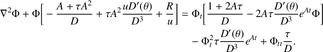(2.2) $$ \begin{align} \nabla^2\Phi+\Phi\bigg[-\frac{A+\tau A^2}{D}+\tau A^2\frac{uD'(\theta)}{D^3}+\frac Ru\bigg] &=\Phi_t\bigg[\frac{1+2A\tau}{D}-2A\tau\frac{D'(\theta)}{D^3}e^{At}\Phi\bigg] \nonumber \\ &\quad -\Phi_t^2\tau\frac{D'(\theta)}{D^3}e^{At}+\Phi_{tt}\frac\tau D. \end{align} $$

The first square bracketed term is autonomous in t when R and D are related by

(2.3) $$ \begin{align} R(\theta)=k^2u+\frac{(A+\tau A^2)u}{D}-\tau A^2\frac{u^2D'(\theta)}{D^3}, \end{align} $$

where $k^2$ is a real valued function of x, independent of t. Thence, in the consequent form of equation (2.2), we have the general form of a PDE that is consistent with the proposed nonclassical symmetry. Noting that $D(\theta )=u'(\theta )$ , if $R(\theta )$ is specified as a function, then equation (2.3) is a second-order nonlinear differential equation for $u(\theta )$ . When $\tau =0$ , it reduces to a first-order differential equation that is also separable when $k=0$ . If the flux potential $u(\theta )$ is specified as a function, then each of the modelling functions $D(\theta )$ and $R(\theta )$ follows directly from $u(\theta )$ by differentiation $D(\theta )=u'(\theta )$ and by explicit algebraic construction in equation (2.3).

When $\Phi _t({\mathbf x},t)$ is identically zero, the reduced equation for $\Phi ({\mathbf x})$ has no coefficients that depend on t. Then there is a consistent reduction of variables. For the remainder of this article, we assume that $k^2$ is simply constant. Then the reduced equation is simply the linear Helmholtz equation

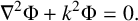$$ \begin{align*} \nabla^2\Phi+k^2\Phi=0. \end{align*} $$

From every member of the infinite dimensional solution space of the Helmholtz equation, a solution can be constructed for the nonlinear hyperbolic reaction diffusion equation (1.1) that has the structure of equation (2.3). However, this does not give all the solutions of equation (1.1), only those satisfying the side condition $u_t=Au$ with $du/d\theta =D(\theta )$ . In that sense, the nonlinear PDE is conditionally integrable. This is to be compared with a classical Lie symmetry, in which case equation (2.2) would immediately be autonomous in t. That is to say, the equation itself, and not just a particular subclass of solutions, would be invariant. Generally speaking, reduction of a PDE by successive classical Lie symmetries leads to an ordinary differential equation and a finite- rather than infinite-dimensional manifold of solutions.

3 Reaction term of Fisher–KPP type

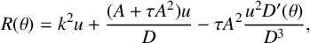
For a model of Fisher–KPP type [Reference Fisher20, Reference Kolmogorov, Petrovsky and Piscounov29], the target reaction function is considered to be the canonical Verhulst form $R(\theta )=s\theta (1-\theta )$ , where the density is dimensionless, having been scaled by the carrying capacity. To approximate the structure of a target reaction function $R(\theta )$ , it is convenient to express equation (2.3) as

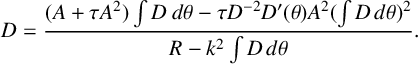(3.1) $$ \begin{align} D=\frac{(A+\tau A^2)\int D~d\theta-\tau D^{-2}D'(\theta)A^2(\int D\,d\theta)^2}{R-k^2\int D\,d\theta}. \end{align} $$

Consider a model of Fisher–KPP type $R=s\theta -s\theta ^2+\mathcal O(\theta ^3);~ D=D_0+\mathcal O(\theta )$ near $\theta =0$ with $D_0>0$ and $s>0$ . Then equation (3.1) implies

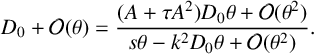$$ \begin{align*}D_0+\mathcal O(\theta)=\frac{(A+\tau A^2)D_0\theta +\mathcal O(\theta^2)}{s\theta-k^2D_0\theta+\mathcal O(\theta^2)}.\end{align*} $$

Taking the limit $\theta \to 0$ in equation (3.1) gives

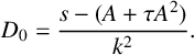(3.2) $$ \begin{align} D_0=\frac{s-(A+\tau A^2)}{k^2}. \end{align} $$

Choose $D_0(\theta )=D(0)$ (constant). Then apply equation (3.1) as a recurrence relation

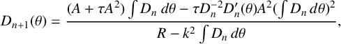$$ \begin{align*} D_{n+1}(\theta)=\frac{(A+\tau A^2)\int D_n~d\theta-\tau D_n^{-2}D_n'(\theta)A^2(\int D_n\,d\theta)^2}{R-k^2\int D_n\,d\theta}, \end{align*} $$

where R is kept at the target $R(\theta )=s\theta (1-\theta ).$ For some cases of the parabolic ( $\tau =0$ ) model with R bounded, such as in the Arrhenius reaction term, this gives a contraction map on $L^\infty $ that converges to the partner $D(\theta )$ that solves equation (3.1). It is not known if this can be a contraction map when $\tau>0$ . In any case, the first iteration gives a useful function $D_1$ from which a useful partner reaction term $R_1(\theta )$ can be constructed explicitly from equation (3.1) by integration:

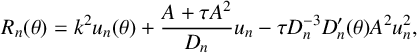$$ \begin{align*} R_n(\theta)=k^2u_n(\theta)+\frac{A+\tau A^2}{D_n}u_n-\tau D_n^{-3}D_n'(\theta)A^2 u_n^2, \end{align*} $$

where $u_n(\theta )=\int _{\theta _\ell }^\theta D_n(\bar \theta )\,d\bar \theta $ . However, $\theta _\ell $ is chosen to be zero so that $R\to 0$ as $\theta \to 0$ , the necessity of which is shown in the sequel. The construction of Broadbridge and Bradshaw-Hajek [Reference Broadbridge and Bradshaw-Hajek5] for $\tau>0$ now extends to $\tau \ge 0$ :

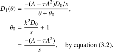$$ \begin{align*} D_1(\theta)&=\frac{-(A+\tau A^2)D_0/s}{\theta+\theta_0}, \\ \theta_0&=\frac {k^2D_0}{s}+1\\ &=\frac{-(A+\tau A^2)}{s}, \quad \mbox{by equation}\ (3.2). \end{align*} $$

Assume $A<0$ . Then,

$$ \begin{align*} u(\theta)=\int _0^\theta D_1(\bar\theta)\,d\bar\theta=\frac{1}{k^2s}(|A|-\tau A^2)(s+|A|-\tau A^2)\log \bigg( \frac{s(\theta+\theta_0)}{|A|-\tau A^2}\bigg) \end{align*} $$

and

$$ \begin{align*} R_1&=\log\bigg(1+\frac{\theta }{\theta_0}\bigg)\bigg[\bigg(\frac{(s+|A|-\tau A^2)}{ s}\bigg)(|A|-\tau A^2)-(|A|-\tau A^2)(\theta+\theta_0)\bigg]\\ &\quad +\tau A^2(\theta+\theta_0)\bigg[\log\bigg(1+\frac{\theta }{\theta_0}\bigg)\bigg]^2=s\theta+\mathcal O(\theta^2). \end{align*} $$

Note that $R_1(\theta )$ has zeros at $\theta =0$ and where $\theta =\bar \theta _c$ such that

$$ \begin{align*}\bigg(\frac{s+|A|-\tau A^2)}{ s}\bigg)(|A|-\tau A^2)-(|A|-\tau A^2)(\theta+\theta_0)+\tau A^2(\theta+\theta_0)\log\bigg(1+\frac{\theta }{\theta_0}\bigg)=0.\end{align*} $$

This transcendental equation can be expressed in normal form as

$$ \begin{align*} we^w=z, \end{align*} $$

where

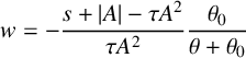$$ \begin{align*} w=-\frac{s+|A|-\tau A^2}{\tau A^2}\frac{\theta_0}{\theta+\theta_0} \end{align*} $$

and

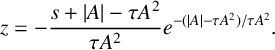$$ \begin{align*} z=-\frac{s+|A|-\tau A^2}{\tau A^2}e^{-(|A|-\tau A^2)/\tau A^2}. \end{align*} $$

Note that as $\tau \to 0$ , $\theta _0\to |A|/s, \bar \theta _c\to 1, z\to 0$ and $w\to -\infty $ . Therefore, the solution is

$$ \begin{align*} w=W_{-1}(z), \end{align*} $$

where $W_{-1}$ is the real negative branch of the Lambert W function [Reference Corless, Gonnet, Hare, Jeffrey and Knuth14]. Then,

$$ \begin{align*} \bar\theta_c+\theta_0=-\frac{s+|A|-\tau A^2}{\tau A^2}\frac{\theta_0}{w}. \end{align*} $$

When $\tau> 0$ , the positive root $\bar \theta _c$ of $R_1$ is now larger than 1. However, we can rescale the dependent variable to $\Theta =\theta /\bar \theta _c$ to achieve a reaction diffusion equation with zero reaction at $\Theta =1$ ,

$$ \begin{align*} \frac{\partial \Theta}{\partial t}+\tau \frac{\partial^2 \Theta}{\partial t^2}=\nabla\cdot[D(\theta(\Theta))\nabla\Theta]+\frac{1}{\bar\theta_c}R(\theta(\Theta)). \end{align*} $$

Note that after rescaling $\theta $ , the governing equation still takes the form of equation (1.1) and the nonlinear coefficient functions still obey a relationship of the form in equation (2.3).

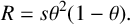
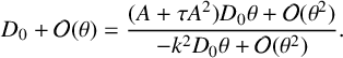
A zero population boundary condition represents lethal over-harvesting in the exterior of a protected reserve. With zero population at a circular boundary $r=a$ , there is a solution of the form

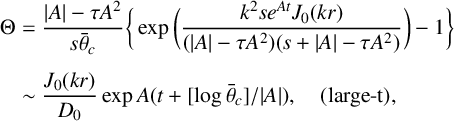$$ \begin{align*} \Theta&=\frac{|A|-\tau A^2}{s\bar\theta_c}\bigg\{\exp \bigg (\frac{k^2se^{At}J_0(kr)}{(|A|-\tau A^2)(s+|A|-\tau A^2)}\bigg )-1\bigg\}\\[5pt] &\sim \frac{J_0(kr)}{D_0}\exp A(t+[\log\bar\theta_c]/|A|),\quad \mbox{(large-t)}, \end{align*} $$

where $k=\lambda _{0,1}/a$ , $\lambda _{0,1}\approx 2.404$ (first zero of Bessel $J_0$ [Reference Skellam39]). For specified linear homogeneous boundary conditions for $u(x,t)$ on a compact connected domain, k is of the form $\lambda /a$ , where the geometric length scale a and the dimensionless factor $\lambda $ depend on the geometry of the domain. For a line segment of length a, $k=\pi /a$ . For a rectangle, $\lambda =\pi $ and a is the hyperbolic root mean square length of sides [Reference Broadbridge and Hutchinson8]. Now consider the Fisher–KPP class with $R=s\theta + \mathcal O(\theta ^2).$ The fundamental relationship in equation (3.2) implies

(3.3) $$ \begin{align} A=\frac{-1+\sqrt{1+4\tau(s-\lambda_0^2D_0/a^2)}}{2\tau}. \end{align} $$

In applications such as no-take areas for conservation within fisheries, it is important that the extinction point $\theta =0$ be unstable. Then it is necessary that $A>0$ which, by equation (3.3), is equivalent to

$$ \begin{align*} a>\lambda \sqrt{D_0/s}. \end{align*} $$

Importantly, this is independent of the delay $\tau $ . In the case $\tau =0$ , this is the well-known criterion for instability of the extinction point, originally obtained by linear stability theory [Reference Skellam39].

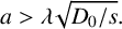
Figure 1 Solvable model of Fisher–KPP type. Parameters used: $A=-1.5, s=1, k=2.4048$ .

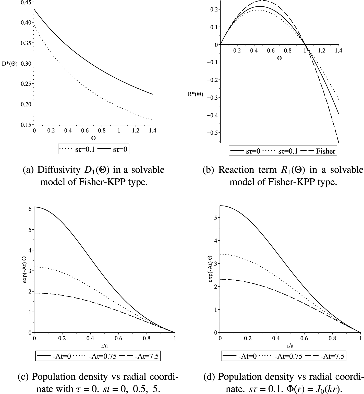
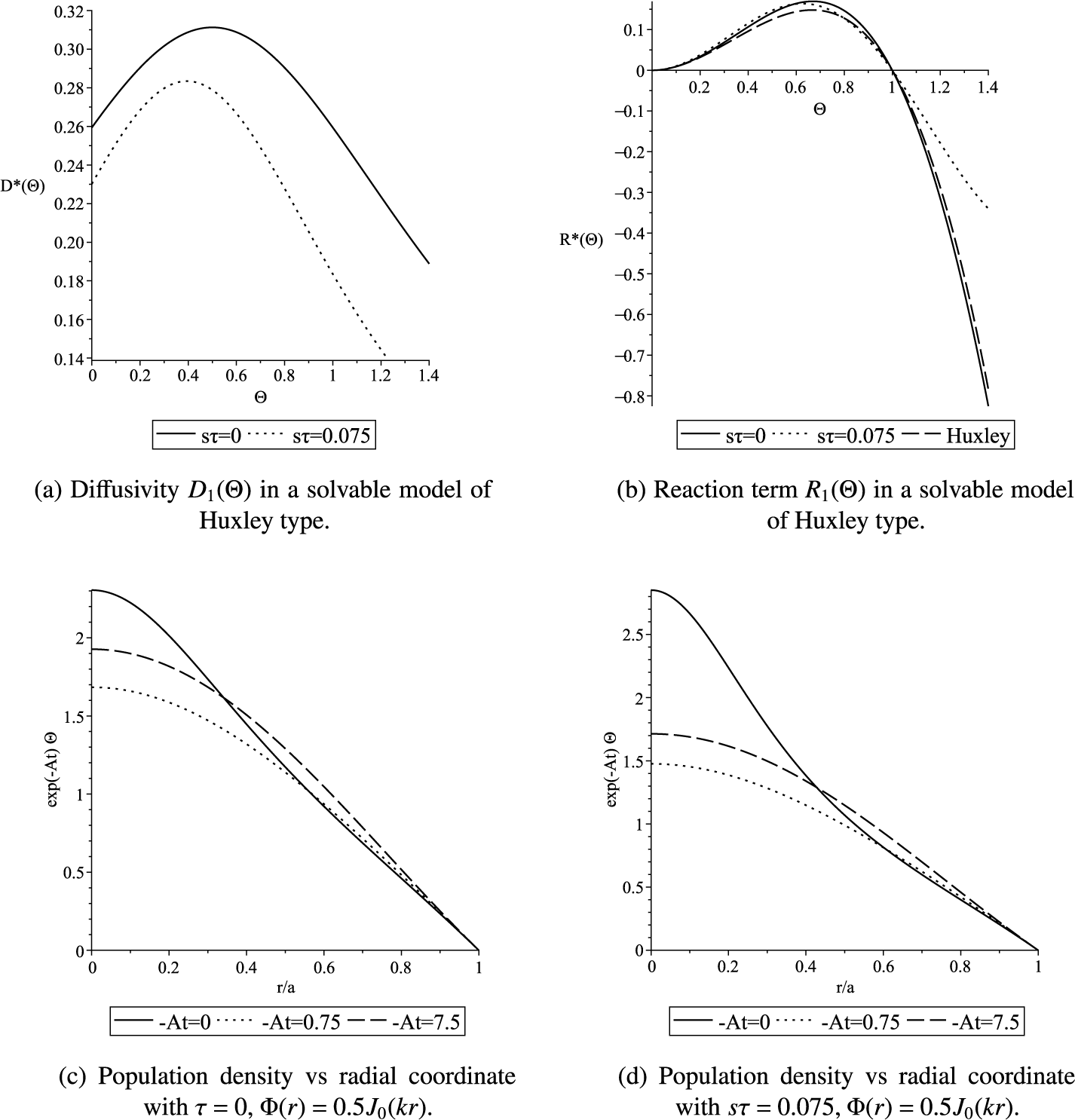
For the example with $\tau =0.1, s=1, ~A=-1.5$ , in Figure 1, the partner diffusivity and reaction functions are plotted as functions of the scaled population density. Note that by equation (3.2), D must decrease with $\tau $ whenever $A\ne 0$ . With larger delay $\tau $ , diffusivity is lower to achieve the same nonzero decay rate $-A$ . Conversely, if both $D_0$ and s were prescribed, decay would be more rapid in the case of larger $\tau $ . In fact, in the first application of the telegraph equation by Heaviside, $\tau $ was proportional to the electrical resistance of the medium.

4 Reaction term of Huxley form with weak Allee effect

The simplest form of an equation with weak Allee effect [Reference Allee and Bowen3] is the Huxley equation (see [Reference Chin12] and the references therein), which has

$$ \begin{align*} R=s\theta^2(1-\theta). \end{align*} $$

Again, it is assumed here that the density has been scaled by the carrying capacity so that it is dimensionless. In fact, this reaction term arises as the growth of a density of a new favourable allele under Mendelian inheritance [Reference Russell38], not the Fisher equation as is frequently supposed (for example, see [Reference Broadbridge, Bradshaw, Fulford and Aldis6]). As a model of population growth, at low population, it has the per-capita growth rate $R/\theta \approx s\theta -s\theta ^2$ increasing from zero, rather than being a positive constant or decreasing from a positive constant, as in the Malthusian and Verhulst models [Reference Iannelli and Pugliese26]. Since the growth rate is not negative near $\theta =0$ , this is a weak Allee effect rather than a strong Allee effect (see for example, Courchamp et al. [Reference Courchamp, Berec and Gascoigne15]). Consider $R=s\theta ^2+\mathcal O(\theta ^3)$ and $D=D_0+\mathcal O(\theta )$ near $\theta =0$ with $D_0>0$ and $s>0$ . Then equation (3.1) implies

$$ \begin{align*} D_0+\mathcal O(\theta)=\frac{(A+\tau A^2)D_0\theta +\mathcal O(\theta^2)}{-k^2D_0\theta+\mathcal O(\theta^2)}. \end{align*} $$

Taking the limit $\theta \to 0$ in equation (3.1) gives the result

$$ \begin{align*} D_0=\frac{-(A+\tau A^2)}{k^2}. \end{align*} $$

Then,

$$ \begin{align*} D_0&=\frac{-\bar A}{k^2}, \quad \bar A=A+\tau A^2, \\[1pt] D_1&=\frac{D_0\bar A}{s\theta(1-\theta)+\bar A}, \end{align*} $$

(4.1) $$ \begin{align} u_1&=\frac{|\bar A|D_0/s}{\sqrt{s/(|\bar A|-s/4)}}\arctan \bigg(\bigg[\theta-\frac 12\bigg] \sqrt{\frac{s}{|\bar A|-s/4}}\bigg) \\[1pt] &\quad +\frac{|\bar A|D_0/s}{\sqrt{s/(|\bar A|-s/4)}}\arctan \bigg(\frac 12\sqrt{\frac{s}{|\bar A|-s/4}}\bigg)\nonumber \end{align} $$

and

$$ \begin{align*} R_1=\frac{k^2}{|\bar A|}s\theta(1-\theta)u_1+\tau A^2 s\frac{k^4}{\bar A^4}(2\theta-1)(|\bar A|+s\theta[\theta-1])u_1^2. \end{align*} $$

From equation (4.1), $\theta \to \infty $ as

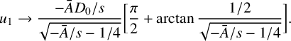$$ \begin{align*}u_1\to\frac{-\bar AD_0/s}{\sqrt{-\bar A/s- 1/4}}\bigg[\frac\pi 2+\arctan \frac{1/2}{\sqrt{-\bar A/s- 1/4}}\bigg].\end{align*} $$

Therefore, the maximum value of $u_1$ must be chosen to be much less than that limiting value. Again, when $\tau>0$ , the positive zero $\bar \theta _c$ of $R_1$ exceeds 1. After rescaling by ${\Theta =\theta /\bar \theta _c}$ , the compatible diffusivity function and reaction function are plotted in Figure 2.

Figure 2 Solvable model of Huxley type. Parameters used: $A=-1.5, s=1, k=2.4048$ .

As expected, again with larger delay $\tau $ , diffusivity is lower to achieve the same logarithmic decay rate $-A$ . Conversely, if both $D_0$ and s were prescribed, decay would be more rapid in the case of larger $\tau $ .

5 Arrhenius combustion

With $\theta $ being the absolute temperature, a heat source is of the form $\rho C R$ , where $\rho $ is density of the medium, C is heat capacity and the rate of temperature increase due to combustion is

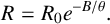$$ \begin{align*} R=R_0e^{-B/\theta}. \end{align*} $$

From the Gibbs canonical distribution [Reference Gibbs22], typically $B=\Delta E/k_B$ , where $\Delta E$ is a molecular activation energy and $k_B$ is Boltzmann’s constant. This reaction function is difficult to handle analytically. It is not an analytic function; all derivatives $d^nR_0/d\theta ^n$ approach 0 as $\theta \to 0$ . In the case $\tau =0$ , the only known exact solution for temperature is that given by Broadbridge et al. [Reference Broadbridge, Bradshaw-Hajek and Triadis7]. The solution requires $k=0$ and $A>0$ ; consequently, the solution is unbounded in both time and space. Given the Arrhenius reaction term, the appropriate solution of equation (2.3) was found to be [Reference Broadbridge, Bradshaw-Hajek and Triadis7]

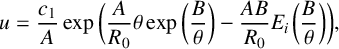$$ \begin{align*} u=\frac{c_1}{A}\exp\bigg (\frac {A}{R_0}\theta\exp\bigg (\frac B\theta\bigg)-\frac{AB}{R_0}E_i\kern1.2pt\bigg (\frac B\theta\bigg)\bigg), \end{align*} $$

where the function $E_i$ is the exponential integral and $c_1$ is an arbitrary positive constant with units K m² s $^{-2}$ . Since $D(\theta)=u'(\theta)$ ,

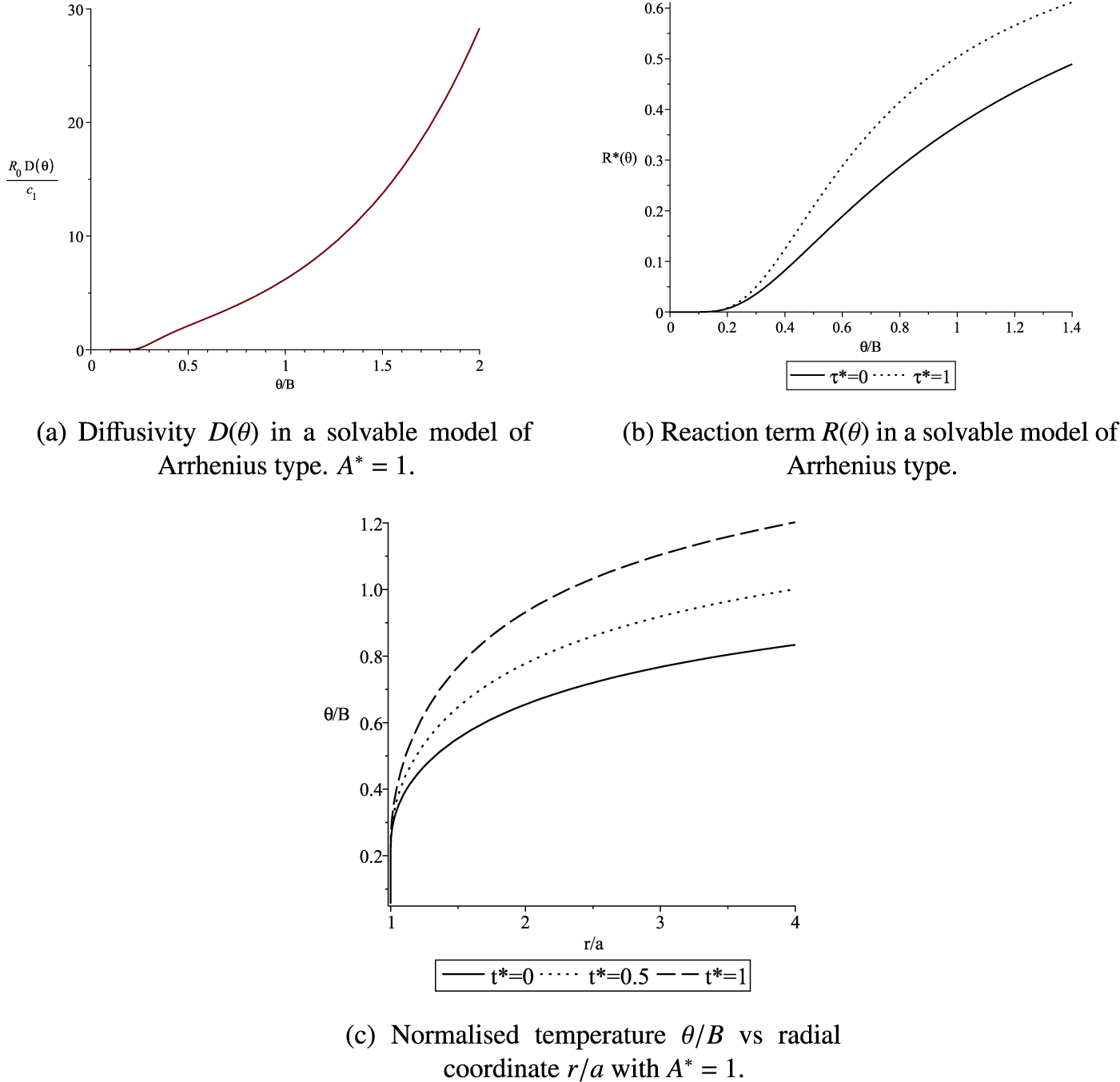
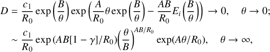$$ \begin{align*} D&=\frac{c_1}{R_0}\exp\bigg(\frac B\theta\bigg)\exp\bigg(\frac {A}{R_0}\theta\exp\bigg(\frac B\theta\bigg)-\frac{AB}{R_0}E_i\kern1.2pt\bigg(\frac B\theta\bigg)\bigg) \, \to 0, \quad \theta\to 0;\\ &\sim \frac{c_1}{R_0}\exp{(AB[1-\gamma]/R_0)}\bigg(\frac\theta B\bigg)^{AB/R_0}\exp(A\theta/ R_0), \quad \theta\to\infty, \end{align*} $$

where $\gamma =0.5772\ldots $ is Euler’s number. More generally, with $\tau \ge 0$ , this diffusivity function has a partner reaction function

$$ \begin{align*} R=R_0[e^{-B/\theta} +BR_0\tau\theta^{-2}e^{-2B/\theta}]. \end{align*} $$

This reaction function agrees asymptotically with the Arrhenius reaction as $\theta \to 0$ and as $\theta \to \infty .$ From the form of the reaction and diffusivity functions, there are intrinsic temperature, time and length scales, namely,

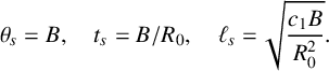$$ \begin{align*} \theta_s=B, \quad t_s=B/R_0, \quad \ell_s=\sqrt{\frac{c_1B}{R_0^2}}. \end{align*} $$

In terms of the dimensionless variables $\vartheta =\theta /\theta _s$ , $t^*=t/t_s$ and $r^*=r/\ell _s$ , equation (1.1) is normalised to

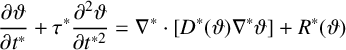$$ \begin{align*} \frac{\partial \vartheta}{\partial t^*}+\tau^* \frac{\partial^2 \vartheta}{\partial t^{*2}}=\nabla^*\cdot[D^*(\vartheta)\nabla^*\vartheta]+R^*(\vartheta) \end{align*} $$

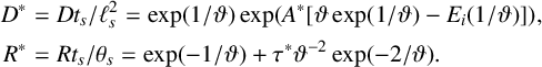
with

$$ \begin{align*} D^*&=Dt_s/\ell_s^2=\exp(1/\vartheta)\exp(A^*[\vartheta \exp(1/\vartheta)-E_i(1/\vartheta)]), \\ R^*&=Rt_s/\theta_s=\exp(-1/\vartheta)+\tau^*\vartheta^{-2}\exp(-2/\vartheta). \end{align*} $$

The dimensionless time lag parameter is $\tau ^*=R_0\tau /B$ . The other dimensionless parameter is $A^*=AB/R_0$ . This is related to the diffusivity at activation temperature by

$$ \begin{align*}A^*= [\log D^*(B)-1/B]/[B\exp(1/B)-E_i(1/B)]. \end{align*} $$

The ratio of the additional reaction component to the Arrhenius reaction is

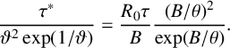$$ \begin{align*} \frac{\tau^*}{\vartheta^2\exp(1/\vartheta)} =\frac{R_0\tau}{B}\frac{(B/\theta)^2}{\exp(B/\theta)}. \end{align*} $$

This approaches 0 at very small and very large $\theta $ , and it attains the maximum value $4R_0\tau /e^2B$ at $\theta =0.5 B$ . This is a small fraction, equivalent to the ratio of the heat released over one collision time to the total heat content of the material at activation temperature. As an example, with $k=0$ , there is an elementary radial solution $u/u_0=\log (r/a)$ ( $u_0$ constant) to the exterior problem with boundary condition $\theta (a,t)=0$ . The isotherms follow exactly from the mapping

$$ \begin{align*} (t,\theta)\mapsto u\mapsto\Phi=e^{-At}u\mapsto r=a\exp(u/u_0). \end{align*} $$

The radial solution is plotted in Figure 3. At the circle $r=a_1>a$ , the radial heat flux density $j(r)$ , which is $-u'(r)$ , satisfies $j(r)/u(r)=-\Phi '(r)/\Phi (r)=-u_0/a_1$ (constant). This may be interpreted as a physical generalisation of a Newtonian cooling law. Whereas the heat flux potential is $u(\theta )$ , the inward heat flow at the boundary is proportional to the potential difference between the local temperature and that of a remote inner point. However, the inward heat flow through a finite boundary is not sufficient to prevent unbounded temperature rise due to combustion throughout the entire external region of infinite area.

Figure 3 Solvable model of Arrhenius type.

In addition to the delay $\tau $ between setting up a density gradient and establishing a flux, there is a separate delay $\tau _2$ between changing a density and changing a reaction rate before a sufficiently energetic collision takes place to overcome the activation energy. At first order in both $\tau $ and $\tau _2$ ,

(5.1) $$ \begin{align} [1+(\tau_2-\tau)R'(\theta)]\frac{\partial \theta}{\partial t}+\tau \frac{\partial^2 \theta}{\partial t^2}=\nabla\cdot[D(\theta)\nabla\theta]+R(\theta). \end{align} $$

Since in the absence of harvesting, epidemics and environmental disasters, it normally takes several generations for a population growth rate to change appreciably, it is assumed that both $\tau R'(\theta )$ and $\tau _2 R'(\theta )$ are small compared to 1. Equation (1.1) may result from the approximation $\tau _2=\tau $ . However, at temperatures well below observed ignition temperatures, the delay $\tau _2$ may be considerably longer than $\tau $ . In applications to populations, an alternative approximation $\tau _2=0$ is implicit in the reaction-telegraph equation studied in [Reference Alharbi and Petrovskii1, Reference Cirilo, Petrovskii, Romeiro and Natti13]. This may apply to some single-cell organisms that multiply rapidly. In that case, the critical domain size increases with $\tau $ [Reference Alharbi and Petrovskii1]. For vertebrates with a long gestation period, typically $\tau _2>\tau $ .

6 Discussion and conclusion

Physical fields that depend on both space and time generally evolve according to PDEs. Most exact solution methods involve reduction to an ordinary differential equation after assuming some symmetry. The most familiar solutions obtained in this way are steady states, uniform states, travelling waves, radial solutions and scale-invariant similarity solutions. For the applicable class of nonlinear PDEs studied here, another type of solution is available, that is, a solution with functional separation in which the time dependence is exponential: $u(\theta )=e^{At}\Phi (x)$ . The reduction is associated with a nonclassical symmetry that does not leave the governing PDE invariant, unless an extra algebraic constraint is added among the coefficient functions. Somewhat surprisingly, the constraint allows an exact solution to be constructed from any solution $\Phi (x)$ to the linear Helmholtz equation. That means that this class of nonlinear PDE is conditionally integrable, yielding an infinite-dimensional space of exact solutions, albeit not the whole set of solutions. The general classification of conditionally integrable PDEs remains largely unexplored.

In particular, in this article, we have concentrated on nonlinear hyperbolic reaction-diffusion equations in two space dimensions, for which, to our knowledge, no space–time-dependent exact solutions have been seen before. In recent times, such equations have been associated with speed-limited diffusion due to a delay $\tau $ between gradients and fluxes. For reaction-diffusion equations of Fisher–KPP type modified by sufficiently small $\tau $ , we produced an exact solution approaching extinction due to lethal boundary conditions on the boundary of a circular domain, that is, not just the small- $\theta $ approximation but the full nonlinear solution. It is well known from population models that such a solution exists only when the domain is smaller than some critical size. Importantly, we showed that the critical domain size does not depend on $\tau $ , therefore, it does not depend on the speed limit.

For population models of Huxley type with weak Allee effect, we again produced an extinction-bound solution within a circle when $\tau>0$ . For this type of model, the linear approximation near the extinction point has zero reaction, so linear stability analysis is not useful for determining the critical domain size. There have been some general qualitative results in that direction, but explicit results on critical domain size are lacking. Such results would be useful for conservation of invertebrate species, such as queen conch that exhibit an Allee effect [Reference Stoner and Ray-Culp40]. When gestation time is large compared to the mobility delay, the governing equation is modified to equation (5.1). The consequences of the gestation delay will be investigated in the future.

For a reaction-diffusion model of single-component combustion, we produced an exact finite-valued but unbounded solution with $\tau>0$ . In the limit $\tau \to 0$ , this reduces to the only known exact solution with standard Arrhenius reaction. When $\tau $ takes realistic small positive values, the relative change to the standard reaction term is bounded and small. As with the actual Arrhenius reaction term that is bounded, blow-up occurs in infinite time, not in finite time as occurs in models with artificial unbounded reaction terms.