


1. INTRODUCTION
Mass balance and ice dynamics govern the geometry of a glacier and its temporal variations. Thus, the inversion of changes in geometry can reveal the combined signal of ice transport and glacier mass balance (Hagen and others, Reference Hagen, Eiken, Kohler and Melvold2005). Especially in inaccessible regions, the analysis of changes in geometry based on remote-sensing investigations provides an alternative to in situ mass-balance measurements. However, glacier wide DEM differencing provides the bulk mass-balance estimates only if the snow and firn density distribution in the accumulation area is known (Rolstad and others, Reference Rolstad, Haug and Denby2009). In addition, DEM calculations based on microwave remote-sensing sensors (e.g. TanDEM-X products) are affected by uncertainties caused by the unknown and variable penetration depth of microwaves in the snow and firn layers (Munk and others, Reference Munk, Jezek, Forster and Gogineni2003; Rott and others, Reference Rott2014).
Local mass balance derived from elevation changes requires knowledge of ice advection in order to remove the elevation effect due to ice dynamics. In the ablation area, where penetration depth plays a minor role, the combination of elevation differences from microwave remote-sensing and surface velocities derived from feature tracking might be suitable to determine local mass balance. This method is mainly hampered by limited temporal availability of remote-sensing imagery for determining the seasonal or annual mass balance.
The outcrop position of stable, englacial isochrones in the ablation zone may provide additional information about the relation between ice melt and surface displacement. We introduce a simple scheme for deriving the local surface mass balance (SMB) from position changes of a tephra-layer outcrop in the ablation zone, using additional surface velocity information and ground-based geometry measurements. The relative displacement of the layer outcrop depends on the surface velocity, the ablation rate and the emergence angle of the layer. This displacement can easily be derived from optical remote-sensing data, which are available for >30 years back in time. We are thus able to reconstruct the local SMB for the outcrop position into the past. In this proof-of-concept study we cover the period 1988 to 2014, based on data from different generations of the Landsat satellites and concentrating on a specific location on the northern part of Mýrdalsjökull. Because tephra-layer outcrops are common on Icelandic glaciers, the knowledge of their emergence angle combined with information about surface velocity and the outcrop displacement enables the reconstruction of local SMB at many locations. Therefore, this new method has the potential to improve the interpretation of local direct mass-balance measurements, by extending the ablation distribution over larger areas.
After describing the field site, the theoretical background is laid for deriving ice velocity components from observed glacier surface markers. A simple flowline model provides the required qualitative evolution of isochrones over time and thus the emergence angle of isochrones in the upper ablation zone. Then the field and remote-sensing measurements and the resulting data are described. The temporal development of local ablation is derived in Sections 6–8, while the potential of the method and its limitations are described in Section 9.
2. SITE DESCRIPTION
The Mýrdalsjökull ice cap is situated in the south of Iceland, with its southern margin only 8–14 km from the coast. The maritime climate of Iceland leads to mass-balance conditions with high amounts of precipitation and comparatively high summer ablation rates at the low glacier termini (Ágústsson and others, Reference Ágústsson, Hannesdóttir, Thorsteinsson, Pálsson and Oddsson2013). The ice cap stretches from ~120 m a.s.l. to an extensive plateau at ~1300–1350 m a.s.l., which is surmounted by some higher peaks along the rim of the volcanic caldera (Fig. 1). The total area of the ice cap was ~586 km2 in 2004 (Jaenicke and others, Reference Jaenicke, Mayer, Scharrer, Münzer and Guðmundsson2006) and the ice volume has been estimated at 140 km3 (Björnsson and others, Reference Björnsson, Pálsson and Guðmundsson2000). The caldera of the underlying Katla volcano forms the basis for the large central plateau of the ice cap. Katla showed three volcanic events during the 20th century with a strong eruption and volcanic fallout during the first of these events in 1918 (Thordarson and Larsen, Reference Thordarson and Larsen2007). This tephra layer was buried in the accumulation area of the glacier, while ice melt and supraglacial water flow redistribute and continuously remove the material from the ablation zone. Today, the outcrop of this internal tephra layer, besides others, is clearly visible on the glacier surface as a narrow black band across the ablation zone, at ~900–1000 m a.s.l. on the northern slope of the ice cap (Sigurðsson, Reference Sigurðsson2010), reaching down to ~700 m a.s.l. in the eastern part of Öldufellsjökull.
Landsat 8 satellite image of Mýrdalsjökull Ice Cap from 12 August 2014. The red curve displays the glacier boundary and the principal drainage units, including debris-covered glacier areas. On the northern lobe, Sléttjökull is composed of the three northernmost sub-basins. The locations of field measurements in 2013/14 are indicated, as well as the flowline profile (blue). Arrows indicate the position of the tephra layer outcrop. Contours are based on a DEM of Iceland compiled by Hans H. Hansen, Fixlanda ehf., Iceland (Lidar data source: Icelandic Meteorological Office and Institute of Earth Sciences, University of Iceland, 2013; DEMs of Icelandic glaciers (dataset)).

Accumulation is extremely high, reaching more than 7000 mm w. e. a−1, while the annual mass balance on the plateau shows a high variability between 2000 mm w. e. and ~6000 mm w. e. (Ágústsson and others, Reference Ágústsson, Hannesdóttir, Thorsteinsson, Pálsson and Oddsson2013). Ice melt is highly variable across the ablation region, reaching up to 10 m w. e. a−1 (Thorsteinsson and others, Reference Thorsteinsson, Waddington, Matsuoka, Howat and Tulaczyk2005). At Sléttjökull, the northern lobe of Mýrdalsjökull, the ice ablation close to the glacier terminus reaches several metres during the summer. In this sector of the ice cap, the equilibrium line varies between ~900 and 1200 m a.s.l., depending on the balance year. In this environment, classical field-based mass-balance monitoring is very challenging (Ágústsson and others, Reference Ágústsson, Hannesdóttir, Thorsteinsson, Pálsson and Oddsson2013).
Our activities focus on Sléttjökull, which is not uniquely defined, as Öldufellsjökull is sometimes included and sometimes not (e.g. Björnsson and others, Reference Björnsson, Pálsson and Guðmundsson2000; Sigurðsson, Reference Sigurðsson2010). We refer to all three sub-basins of the northern Mýrdalsjökull as Sléttjökull (Fig. 1). This part of the ice cap is characterized by a smooth surface geometry and radial ice flow. It covers an area of ~156 km2, with the highest and lowest elevation at 1446 and 434 m a.s.l., respectively (based on our investigations). The longest flowline in this ice cap sector is ~12 km.
3. THE TEPHRA LAYER OUTCROP AND ITS RELATION TO LOCAL SMB
Tephra from volcanic eruptions is frequently deposited on the surfaces of Icelandic glaciers. These layers are incorporated into the glacier by snow accumulation and represent time markers, usable for subsequent investigations. The incorporation mainly depends on the mass balance after deposition of the tephra. Tephra layers on clean ice can easily be washed away by strong rain. Intense ice melt redistributes the material on the glacier surface, although thick ash layers can reduce ice melt considerably due to the reduction of heat transfer towards the ice surface (Juen and others, Reference Juen, Mayer, Lambrecht, Wirbel and Kueppers2013). Tephra deposited in the accumulation area is buried by snowfall during the accumulation seasons. In this way, the tephra layer is incorporated in the glacier and migrates with the snow towards deeper levels. Historical tephra layers, therefore, are only visible at their outcrop somewhere in the ablation zone. Our observations at Sléttjökull show that the width of this outcropping ash layer is restricted to some tens of metres (depending on the original layer thickness), because the compact layer is continuously eroded and redistributed by rain, wind and ice melt, especially at its lower edge. Downstream of the outcropping ash layer, the volcanic material forms isolated ash cones, while rain and meltwater washes most of the material away (Fig. 2). The cones demonstrate the effect of reduced ice ablation underneath ash deposits thicker than a critical thickness, but these anomalies have no significant effect on the total ice ablation.
Left: Tephra layer outcrop of the 1918 Katla eruption in the region of the field work at Sléttjökull (at the station LGPS). Right: Ash cone downstream of the tephra layer outcrop (Photo: J. Jaenicke, 2013).

The location of the well-defined tephra outcrop is the combined result of ice movement and ablation. Assuming a constant layer inclination in the uppermost part of the glacier ice, the layer outcrop position moves with the ice from location s(t 1) to s(t 2) during the time span t 2 −t 1 in Figure 3 and is at the same time affected by ice ablation, which uncovers parts of the tephra layer upstream of the original outcrop location. Dependent on the relation between ice velocity and ablation rate, this outcrop position lies upstream or downstream of the initial position: downstream, if the melt rate is less than the vertical component of the ice flow (elevation difference between the arrowheads s(t 1) and s(t 2): u h tan α s), upstream if the melt rate is higher. The upward or downward movement of the ice at the surface has no influence on the horizontal position of the ash outcrop, as can be seen in Figure 3. This velocity component only shifts the surface at time t 2 (blue dashed line) and the layer outcrop x a(t 2) vertically to the dotted blue line.
Schematic diagram of the components influencing the apparent tephra layer displacement, based on the field observations at the tephra outcrop of the 1918 eruption on Sléttjökull. The horizontal axis originates at the ice divide and is oriented along the ice flow. The light blue line represents the glacier surface at time t 1, with the layer outcrop at x a(t 1). The emergence angle of the tephra layer with respect to the surface is α and the surface inclination from the horizontal is αs. The stake s(t 1) (and the layer outcrop x a(t 1)) are moved by ice transport to s(t 2), while the surface is lowered by ice melt to the dashed blue line during the same time span. Due to this removal of ice, the outcrop position is shifted to the location x a(t 2) and the tephra layer apparently moves upstream. The vertical ice velocity at the surface lowers the surface (dashed blue line) to the position of the dotted blue line, while x a(t 2) does not change its horizontal position.

For a given angle α between the ice surface and the tephra layer and a surface slope α s, the apparent tephra layer displacement x d = x a(t 2)–x a(t 1) depends on the ablation a i and the horizontal ice velocity u h:
 $$x_{\rm d} = u_{\rm h}\Delta t + \displaystyle{{a_i\Delta t} \over {\tan (\alpha - \alpha _{\rm s}) + {\rm tan}\; \alpha _{\rm s}}},$$
where x d is positive downstream (along the direction of the x-axis), u h is thus positive for down-glacier movement and a i is taken negative for ablation.
Therefore, the ablation just upstream of the tephra outcrop can be determined from measurements of the horizontal surface velocity and the displacement of the tephra layer outcrop, if α and α s are known. Reformulating Eqn (1) leads to an estimate of the ice ablation dependence on the observed apparent tephra layer displacement x d:
 $$a_i = (x_{\rm d} - u_{\rm h}\Delta t)({\rm tan}(\alpha - \alpha _{\rm s}) + \tan \alpha _{\rm s}).$$
The surface velocity and the layer displacement can be derived from remote-sensing observations applying feature tracking. At the same time it is possible to determine the surface slope from DEMs. The emergence angle of the tephra layer in the ice can be determined by geophysical methods, for example GPR profiling. Because the applicability of the method depends critically on accurate knowledge of the tephra layer emergence angle, special attention should be given to its determination. Assuming an accuracy of ±0.1° for the tephra layer emergence angle, the error of the resulting melt induced outcrop displacement is ~±6%. To obtain this accuracy the tephra layer elevation difference needs to be measured with a precision of 4 cm over a horizontal distance of 20 m. If the tephra layer depth in the ice is derived by GPR with a frequency of 600 MHz, the vertical resolution of the radar signals is ~9 cm. This implies a need for a profile at least 45 m long, in order to obtain the emergence angle with sufficient accuracy.
4. INTERNAL LAYER EMERGENCE FROM A SIMPLE MODEL
A tephra layer is only parallel to the glacier surface during deposition. In the accumulation area the layer is buried by accumulating snow, and deformed by the ice movement. In the ablation area, tephra will stay at the surface and is removed over time. In the first few years after deposition, the inclination of the tephra layer with respect to the glacier surface at its emergence is very small, but it will increase. If this angle is large enough, the outcrop location will start to move down-glacier even for high-ablation rates (Eqn (1)). We applied a 1-D simple flowline model to the flowline on Sléttjökull, which contains our field site LGPS (Fig. 2), in order to investigate the temporal changes of the emergence angle. The model is very similar to the one used by Brandt and others (Reference Brandt, Björnsson and Gjessing2005), along an almost identical profile. We used a combination of SMB values from the available observations (Brandt and others, Reference Brandt, Björnsson and Gjessing2005; Ágústsson and others, Reference Ágústsson, Hannesdóttir, Thorsteinsson, Pálsson and Oddsson2013; our own ablation measurements) and assumed steady state for simplicity. This assumption is justified, because we only want to investigate the qualitative shape of shallow tephra deposits upstream from the emergence location and no mass-balance data exist. The surface elevation is taken from the elevation model of Hans H. Hansen, Fixlanda ehf, while the ice thickness was extracted from Björnsson and others (Reference Björnsson, Pálsson and Guðmundsson2000).
With the mean horizontal velocity:
 $$\overline {u_{\rm h}} = \displaystyle{{2A} \over {n + 2}}(\rho g)^nH^{n + 1}(\sin \alpha _{\rm s})^n$$
and the assumption of steady state (emergence velocity equals the SMB) it is possible to calculate the particle paths within the glacier and reconstruct the position of the tephra layer. Here, A is the rate factor in Glen's flow law (taken to be 5 × 10⁻²⁴ s−1 Pa−3; Cuffey and Paterson, Reference Cuffey and Paterson2010), n (3) is the flow law exponent, ρ (910 kg m−3) is the ice density, g (9.81 m s−2) the acceleration due to gravity and H (m) the ice thickness. In addition, firn densification is neglected, and the depth is given in ice equivalent (constant density). For the Sléttjökull flowline, the evolution of the tephra layer is shown in Figure 4. This simple model demonstrates that the tephra layer slope is close to horizontal during the past decade just upstream of the outcrop region.
Simple modelling of the englacial tephra layer geometry from the eruption in 1918 in 10 year steps, calculated by a generalized flowline approach (Eqn (3)) and hypothetical steady-state conditions. The tephra layer is buried gradually in the accumulation zone (coloured curves from blue to green) beneath the steady glacier surface (black) and it emerges at the surface downstream of the equilibrium line, where it will be eroded by rain and ice melt. The red curve shows the path through the ice cap of a tephra particle deposited at the uppermost location of our flowline model through the ice cap.

5. FIELD DATA AND REMOTE-SENSING INVESTIGATIONS
In order to test our hypothesis we collected necessary data of ice movement, ice geometry and melt on the Séttjökull flowline close to the tephra layer outcrop in 2013 and 2014 in the framework of the IsViews project (application of new methods based on high-resolution remote-sensing imagery for the early warning of subglacial volcanic eruptions in Iceland; Jaenicke and others, Reference Jaenicke2014). From remote-sensing data we derived the history of the tephra layer outcrop position and the surface flow field. In addition, analysis of DEMs, derived from satellite data, enables the quantification of the general elevation changes and bulk mass balance during the period of field data acquisition.
6. RESULTS FROM FIELD DATA
A GPS receiver was installed at the LGPS location (596239 E, 7071918 N UTM 27N at 945 m a.s.l.; Fig. 1) on a tripod, drilled into the ice, ~30 m upstream of the tephra layer boundary on 12 August 2013. A low-cost single frequency L1 receiver collected code and phase observations for 2 h each day and GPS reference station data of the ISGPS network (Geirsson and others, Reference Geirsson2006) were used to calculate the differential tripod positions. This experiment lasted only for 33 d, because the set-up was damaged. Nevertheless, it provided a reliable horizontal surface velocity of 21.7 m a−1 (azimuth 19.4°) for the measuring period. During set-up and while visiting the site in the next summer on 9 August 2014 the position of the tripod was also determined by GPS, using geodetic dual frequency receivers. The annual horizontal surface velocity resulted to 13.4 m a−1 (azimuth 13.2°) and the vertical displacement of the GPS antenna was −1.49 m during this year with an accuracy of a few centimetres. The late summer velocity in 2013 is thus a factor of ~1.6 higher than this annual velocity. This indicates that seasonal basal sliding plays a considerable role in this region of the ice cap. The azimuth of the ice flow changes slightly between the annual mean flow and ice flow in the summer months, influenced by basal sliding. The difference between vertical stake movement and the vertical component of the ice flow (uh tan αs) results in a vertical ice velocity at the surface of −1.49 – (−0.68) = −0.81 m a−1.
Ablation was measured at two additional locations along, but slightly uphill of the tephra layer outcrop in clean ice, using wooden ablation stakes (locations WABL and EABL in Fig. 1 and Fig. 6), as well as 1.5 km further downstream (location LABL) at ~850 m a.s.l. in largely clean ice (not in the tephra layer). While mean annual ice melt was 1.71 m a−1 at the layer outcrop, the ice melt at the lower site was 3.88 m a−1 from August 2013 to August 2014.
Measurements of the tephra layer at the outcrop positions showed a layer thickness of 10–15 cm. This tephra layer was traced inside a crack in the ice cap for ~21 m in horizontal distance along the ice flow direction and its depth below the surface was measured manually. The emergence angle with respect to the surface was 2.2° ± 0.3°. The surface slope along the flowline (over a distance of 280 m) was measured as 2.9° ± 0.4°, so that the tephra layer has a slope of 0.7° ± 0.5° with respect to the horizontal. The emergence angle is the central parameter for the surface mass-balance reconstruction, because it needs to be determined in the field (or e.g. by airborne radar survey). We used the measured emergence angle for our analysis, but corrected it for the temporal variation according to the model results from the previous section. The temporal variation of the layer inclination of 0.02° a−1 is rather small, as can be seen from the flowline experiments in Figure 4.
7. REMOTE-SENSING DATA AND DERIVED PARAMETERS
The tephra band is clearly visible in optical satellite imagery (Fig. 2). Thus, the horizontal displacement between different scenes can be measured, taking the predominant flow direction into account. Satellite images of the Landsat satellites from 1988 until 2014 were used for this investigation and displacements were measured on five adjacent flowlines near the LGPS location. The mean value of the displacements on the five flowlines was used to calculate the apparent tephra band velocity. The results are given for the time periods with available Landsat images in Table 1. The accuracy of the tephra band identification is one pixel, which results in the errors given in the table.
Mean apparent surface velocity of the tephra band outcrop in the area of LGPS based on Landsat imagery
Positive displacements are downstream and calculated relative to the position of the tephra layer outcrop in 1988.
Surface displacements were derived from optical satellite images of the RapidEye satellites. The imagery has a ground resolution of 6.5 m and five spectral bands. We used the CosiCorr correlation software (Leprince and others, Reference Leprince, Barbot, Ayoub and Avouac2007) to derive the displacements between image pairs (Fig. 5). Downstream of the tephra layer, the surface conditions change considerably and the bare ice and ash cone landscape allows a good correlation of features. The resulting horizontal velocity at the LGPS location close to the tephra band is ~13 ± 2 m a−1 for the period 10 September 2011–01 August 2012, which is very close to the DGPS derived velocities of 13.4 m a−1 for the period August 2013–August 2014. Upstream of the tephra band the correlation method does not work satisfactorily due to the smooth firn surface.
Surface velocities (m a−1) from 10 September 2011 to 01 August 2012, derived by feature tracking from Rapid Eye imagery. Velocity vectors are only shown in areas with reliable and dense feature tracking results. The blue curve represents the true flowline, while the orange line is the idealized flowline for modelling purposes.

Microwave imagery of the TanDEM-X mission with an original ground resolution of 6 m for a time span of 1 year (June 2013 until June 2014) and over the main ablation season in 2014 (1 June–28 August) were available for this study. The acquisitions were processed as RawDEMs at the German Aerospace Centre (DLR), using the operational Integrated TanDEM-X Processor (Rossi and others, Reference Rossi, Rodriguez Gonzalez, Fritz, Yague-Martinez and Eineder2012). Compared with the final TanDEM-X DEM product, for which a considerable number of acquisitions is merged and manually edited, the individual RawDEMs each represent a single time and can therefore be used to investigate temporal height changes, although, not completely free of height ambiguities. Existing corner reflectors on stable ground near the ice cap, deployed in 1995 (Bacher and others, Reference Bacher, Bludovsky, Dorrer, Münzer, Altan and Gründig1999), were used for accurate co-registration (Nuth and Kääb, Reference Nuth and Kääb2011) and elevation calibration of the different RawDEMs. The individual elevation models are also compared in flat, stable and ice free regions around the ice cap in order to assess the elevation accuracy. The mean elevation change in these test areas is <0.5 m, which we take as the mean error for stable ground. Raster-based differences of these DEMs provide elevation changes, which can be summarized as volume changes in individual drainage basins of the glacier.
The elevation models based on the TandDEM-X data were resampled to a grid resolution of 120 m over the glacier area in order to obtain representative mean elevations along the chosen flowline, excluding small-scale local surface changes. For the considered 1 year period, from June 2013 to June 2014, an elevation gain was observed on this profile above 1040 m a.s.l., while below this altitude the surface shows a lowering (Fig. 6). This elevation change varies smoothly from 2.5 m at the highest elevation of the glacier to −3.5 m close to the glacier margin. For the main ablation season in 2014, a more or less homogenous surface lowering of ~−6 m occurs over 3 months.
Surface elevation change (right axis) derived from TanDEM-X imagery for the time span June 2013–June 2014 (light blue/red curves), winter 2012/13 (November until May, orange curve) and summer 2014 (1 June–28 August, blue curve). The surface elevation along the flowline from the ice margin to the caldera rim is shown as dark blue curve (left axis).
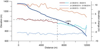
Since no scenes are available for calculating the corresponding winter elevation change in 2013/14, elevation changes were derived for the preceding winter 2012/13. Between November and May, elevation changes from ~3 m close to the margin and up to 10 m at the upper end of the flowline are observed. These findings compare very well with field observations of the general accumulation on this glacier section (Ágústsson and others, Reference Ágústsson, Hannesdóttir, Thorsteinsson, Pálsson and Oddsson2013).
8. SMB RECONSTRUCTION
The local SMB is determined according to the concept laid out above. Usually this determination requires repeated site visits and stake measurements. The existence of englacial tephra layers as a stable time marker allows us to solve the relation between the 3-D velocity field and the time-dependent surface elevation. So long as the surface slope and the emergence angle of the tephra layer are known, calculating the ablation only requires the surface velocity and the apparent tephra layer displacement, two variables that can be derived from remote-sensing data.
The mean SMB was calculated according to Eqn (2) and is presented in Table 2 for the image acquisition dates of Table 1.
Reconstructed tephra layer emergence angle from the measurements in 2014 and the flowline model and resulting mean SMB (m a−1) for the periods covered by remote-sensing imagery
Here, the error is calculated for uncertainties in the displacement deterination based on the remote-sensing imagery. Mean annual mass-balance values for similar periods are presented for comparison from Hofsjökull SW, the closest glacier with a mass-balance record covering almost the same time period (1999–2014; data from WGMS, 2015). An emergence angle uncertainty of 0.2° will add an additional error of 11% to the results.
Obviously, positive SMB cannot be estimated from the apparent displacement of tephra layer outcrops, because the tephra layer is not visible underneath the accumulated snow. For the period 13 September 2011–13 July 2012 the second image is from mid-July, when the snow had just disappeared, as can be seen on the image, while no ice melt occurred. Therefore, it is likely that this period does not cover ice melt at all and the calculated value of 0.39 m a−1 indicates accumulation conditions. The absolute value, however, does not represent an accumulation value, because the method is not valid for accumulation conditions. For the period 09 August 2010–13 September 2011, the large melt rates are probably due to the positive effect of the Eyjafjallajökull eruption, in spring 2010, on the ice ablation (Björnsson and others, Reference Björnsson2013). This effect is also seen in the mass-balance series of Hofsjökull SW. The period 2010–12 (not shown in the table), covering almost two complete years, shows a mean ablation rate of −2.19 m a−1, which is similar to the results for the multi-year ablation rates before and after this period (Table 2). The comparison of the remote-sensing observation period 13 July 2012–12 August 2014 with the field measurements in 2013 and 2014 (which cover almost exactly a full year) results in similar magnitudes. The ablation rate over the 2 year period is −1.65 m a−1, while the second year shows a measured SMB of −1.71 m a−1.
With the characteristic horizontal surface velocity of ~13 m a−1 at the recent tephra layer outcrop position, the tephra layer was transported with the ice ~340 m towards the glacier margin since 1988, while the apparent displacement was almost 460 m upstream. The simple flowline experiment (Fig. 4) indicates that the slope of the englacial tephra layer did not change significantly during this period and over this distance. Also the surface slope very likely did not change considerably in the same period. Therefore, the calculations of the SMB are representative for the given periods back until 1988 and indicate that the mass balance, at least on the northern slope of Mýrdalsjökull, was decidedly less negative in the 1990s than in the most recent 14 years. These results fit rather well with the observations at Hofsjökull, supporting the validity of our study.
We also want to compare the local conditions with the basin wide volume balance, estimated for the available TanDEM-X observation period. This sector wide information, including the magnitude of seasonal elevation changes in the ablation and accumulation region, provides a general framework for understanding the relative magnitude of the reconstructed local SMB from the tephra band analysis. For the investigated Sléttjökull sub-basin, encompassing our test profile, the mean height change is −0.54 m from June 2013 to June 2014, assuming that the penetration depth of the X-band radar is similar and small in June 2013 and 2014 during the same season and wet-surface conditions.
The mean elevation change in the ablation area of the sub-basin was −1.54 m over an area of 34.9 km2, while in the accumulation area the respective results are 1.02 m over an area of 21.8 km2. Based on the uncertainties of the representative layer density in the accumulation zone, the overall mass balance can only be estimated to a certain degree of accuracy. A full adaptation of the vertical density profile according to Sorge's law (Bader, Reference Bader1954) is not very likely for an elevation gain over 1 year only. The application of a simple densification approach, with a constant density gradient between the surface and the firn/ice transition depth (assumed to be ~30 m depth, T. Jóhannesson, personal communication 2016), results in a representative surface layer density between 550 and 720 kg m−3. Using these values as the limits of density variation, the calculations result in a clearly negative specific net balance of the sub-basin of −0.64 to −0.57 m w. e.
The winter balance 2012/13 (November–May) is not easy to derive (see Fig. 5 for the elevation change along the flowline), due to large uncertainties in the penetration depth of the X-band radar in the winter snow and the unknown snow density. The apparent elevation change varies from 3.4 m near the glacier margin to ~10.4 m at the upper end of the flowline. The measured mean snow accumulation a few kilometres west of the upper end of our profile is 9.3 m for the period 2007–12 (Ágústsson and others, Reference Ágústsson, Hannesdóttir, Thorsteinsson, Pálsson and Oddsson2013; location M2). This is in good agreement with our derived elevation change for the winter 2012/13. The local winter balance in the period 2007–12 was 5.0 m w. e., with a mean density of ~540 kg m−3. The elevation change derived from the TanDEM-X data during the summer period, June to end of August 2014, is surprisingly constant at ~−5.8 m.
While the elevation change in the lower part of the glacier very likely represents ice melt only (with a changing contribution from dynamic lowering), it results from a combination of melt and compaction of the snow and firn layer in the upper part of the glacier. Therefore, it is not possible to interpret the elevation change signal during the summer months in terms of mass change without additional information, like meteorological data and depth/density profiles.
9. CONCLUSIONS
Given the scarcity of the database of past elevation change on the northern slope of Mýrdalsjökull, we searched for a method to reconstruct these elevation changes from available parameters. The volcanic activity in Iceland episodically produces suitable markers for such investigations. Volcanic tephra layers, buried in the accumulation region of the glaciers, reappear in the ablation zone with varying emergence angle. Depending upon this angle, the horizontal ice velocity and the ablation rate, the emergence position moves either up- or down-glacier. The surface position of older volcanic horizons, with larger emergence angles, tends to move down-glacier even for large ablation rates. The chosen example of a volcanic surface marker, close to, but downstream of the equilibrium line, demonstrates that mean ablation rates for multi-annual time spans can be reconstructed from the apparent tephra band displacement with some basic assumptions. A critical item of information is the emergence angle, which needs to be measured in the field. GPR measurements easily detect such horizons. In our approach, we change this angle slightly during time, according to results from a simple flowline model.
For investigations further into the past a temporal reconstruction of the emergence angle with a numerical model, calibrated by in-situ measurements, is an option. Remote-sensing imagery provides the required information about surface velocities and apparent tephra band displacement with a sufficient accuracy. It should be noted, however, that only multi-year elevation changes are significant, because small-scale surface variations might obstruct a clear tephra band displacement signal. On the other hand, this simple method allows the reconstruction of SMB across a large part of the ablation zone, as long as suitable tephra horizons are available as markers and the emergence angles are known. Interestingly, the vertical surface velocity is not required for this analysis, because this component of the velocity field does not change the tephra band emergence location. Because tephra deposits are widespread on Icelandic glaciers (Larsen and others, Reference Larsen, Gudmundsson and Björnsson1998), this method could allow a detailed reconstruction of the SMB for the ablation zone of a number of ice caps. Apart from existing remote-sensing imagery for the glaciers, an airborne radar survey could provide the required emergence angles and the local geometry for such an analysis.
The analysis of results from different data sources shows that the northern part of Mýrdalsjökull has a negative mass balance during recent years. The ice flux therefore is clearly out of balance with the SMB. A local SMB of −1.65 m a−1 over the 2 year period 2012–14 (Table 2) compares with a basin wide mass balance of ~−0.6 m a−1 for 2013/14, based on DEM differencing. The according mean mass balance of Hofsjökull SW of −0.465 m a−1 (0.06 for 2012/13 and −0.99 for 2013/14) is in the same magnitude. The elevation differences calculated from TanDEM-X data demonstrate that even for negative net mass balance the elevation in the accumulation zone increases, at least for the mass-balance year 2013/14. If this situation prevails for a longer period the velocity increases and thus an enhanced mass flux from the accumulation region should compensate this additional mass input.
Here, we demonstrated the general idea and the proof-of-concept for our method, but there is still room for improvement. A more accurate determination of the local velocity field will improve the results. In addition, the influence of a transient change of the elevation model on the results should be investigated. So far, only a static recent glacier geometry has been used, because older DEMs were not available. Given suitable marker layers across the ablation zone, it should be possible to derive a distributed SMB for such regions for at least the Landsat satellite image era back to the early 1980s, or even further back by using declassified Corona and Argon imagery.
ACKNOWLEDGEMENTS
The Bavarian Ministry of Economic Affairs and Media, Energy and Technology is gratefully acknowledged for funding the project IsViews (Iceland subglacial Volcanoes interdisciplinary early warning system, ID 20-8-3410.2-15-2012). We thank the BlackBridge AG for providing RapidEye imagery within the DLR/RESA proposal ID 619. The German Aerospace Centre (DLR) is acknowledged for providing TerraSAR-X and TanDEM-X data within the IsViews project (TDX-CoSSC Science Proposal OTHER2375). Ágúst Guðmundsson, Fjarkönnun ehf., is gratefully acknowledged for his support with the organization of the field work, as well as the Icelandic Centre for Research (Rannís) for providing the research permit. We thank Tómas Jóhannesson for helpful comments and suggestions on an earlier version of the manuscript. We are grateful to G. Cogley, one anonymous reviewer and the Scientific Editor H. A. Fricker whose constructive comments considerably improved the manuscript.


 Open access