3.2.1 The construction

We start our construction with a Poncelet m-gon ( $m\geq 7$ ), and consider the lines $L=(l_1, \ldots , l_m)$ that support its edges. Let s be the greatest integer strictly below $m/2$ . Consider the following intersections between those lines, organised into s rings of m points

$$\begin{align*}P_1=\wedge_{1}(L), \ldots , \ P_s=\wedge_{s}(L) \end{align*}$$

along with the points of tangency $P_0=\wedge _{0}(L)$ . Note these points P are Poncelet grid points; they are not the same points P that we are using to construct the configuration in the Construction 1 above.

From the Poncelet grid theorem (Theorem 2.1) we know that the points of each ring $P_i$ lie on a conic $\mathcal {C}_i$ . All conics are co-dependent with respect to the others. (Remark: up to projective transformation they could be represented by a collection of confocal conics).

Now, we pick three distinct natural numbers $a,b,c$ between $1$ and s (inclusive). We focus on the rings $P_a$ , $P_b$ and $P_c$ , and draw tangents to the corresponding conics $\mathcal {C}_a$ , $\mathcal {C}_b$ , $\mathcal {C}_c$ . In our notation those three rings of tangents are

$$\begin{align*}L_a= \vee_{0}\cdot\wedge_{a} (L),\ \quad L_b= \vee_{0}\cdot\wedge_{b} (L),\ \quad L_c= \vee_{0}\cdot\wedge_{c} (L).\ \end{align*}$$

The situation is illustrated in Figure 10. There $n=10$ . We labelled the points on one line with the indices of the corresponding rings. The three rings selected are $P_2$ , $P_3$ and $P_4$ , coloured in blue, green and red, respectively.

Amazingly, the construction is essentially already finished at that point. We have:

The situation is illustrated in Figure 11. There the lines of Figure 10 are extended, and we ‘‘zoom out’’ to show all intersection points. In the present situation we obtain a $(30_4)$ configuration that corresponds to the construction $10\#(2,3;4,2;3,4)$ beginning with the green points. Observe that our choice of $a,b,c$ again occurs as parameters here.

3.2.2 A local incidence lemma

We now consider one specific quadruple concurrence at one specific point of the $(3m_4)$ configuration. Since the situation is totally symmetric it is sufficient to prove the occurrence of one such concurrence to show the existence of all $3m$ such concurrences. Figure 12 highlights the core of the situation, around one of the quadruple intersections of the green and blue lines.

Figure 12

Situation that plays a role for one of the $3m$ four-fold incidences.

Figure 12 Long description

The figure emphasises a single local neighborhood of the incidence configuration constructed in Figures 10 and 11. Four tangent lines belonging to two selected point rings are highlighted around one quadruple intersection. The surrounding points, tangency points, and supporting conics show the local geometric relations responsible for the incidence. Since every quadruple intersection of the full configuration is equivalent by symmetry, the proof reduces to establishing this single local configuration. Figure 12 therefore isolates the essential geometric mechanism underlying Theorem 3.1.

The crucial fact we need to prove for our construction to work is (loosely speaking) ‘‘Whenever the local situation in Figure 12 comes from a Poncelet grid, then the two green and two blue tangents meet in a point’’. In essence, this is a statement about a local incidence configuration. For this we consider four lines $l_0,\ l_a,\ l_b, \ l_{a+b}$ from a Poncelet grid L and show that they locally generate this incidence pattern. From Theorem 2.1 we know that the points in $\wedge _i(L)$ lie on conics $\mathcal {C}_i$ . The following lemma isolates the core incidence pattern.

In fact we may consider the Poncelet subchains

$$\begin{align*}l_0,l_a,l_{2a},l_{3a},\ldots \quad\text{and}\quad l_b,l_{a+b},l_{2a+b},l_{3a+b},\ldots \end{align*}$$

as two different Poncelet chains supported by the same conics.

This highlights the fact that the essence of the last lemma is more of a continuous nature in which b might even vary smoothly. The situation is illustrated in Figure 13. The two Poncelet chains are coloured red and cyan. A self-contained proof of this lemma by direct calculation is presented in Appendix A of this article. The spirit of that proof is very much based on a coordinate-level approach and uses invariant theoretic arguments. In that sense it is similar to the approaches we take in the companion paper [Reference Berman, Gévay, Richter-Gebert and Tabachnikov8]. Theorem 3.1 can be directly derived from Lemma 3.2:

Proof of Theorem 3.1

We only focus on the occurrence of one quadruple coincidence, since the rest follows by symmetry. We defined $L_a=\vee _{0}(\wedge _{a}(L)), L_b=\vee _{0}(\wedge _{b}(L)) $ for an initial collection $L=(l_0,l_1,l_2,\ldots )$ of lines of a Poncelet polygon. The role of the two sequences in Lemma 3.2 is played by the two subsequences

$$\begin{align*}(l_i,l_{i+a},l_{i+2a},l_{i+3a},\ldots)\quad \mathrm{ and }\quad (l_{i+b},l_{i+b+a},l_{i+b+2a},l_{i+b+3a},\ldots),\end{align*}$$

with i being the index of an initial point. As usual, indices are counted modulo m. Both sequences are Poncelet chains with respect to the same conics: the circumscribed conic $\mathcal {X}$ and $\mathcal {B}=\mathcal {C}_a$ , the conic on which the points $\wedge _{a}(L)$ lie. Similarly, the intersections of $l_{i+k\cdot a}$ and $l_{i+b+ k\cdot a}$ lie on the conic $\mathcal {G}=\mathcal {C}_b$ for $k=0,1,2,\ldots $ . By a suitable index shift we may assume $i=0$ . Applying Lemma 3.2 after this shift we get

$$\begin{align*}l_i\wedge l_{i+a},\quad l_{i+b}\wedge l_{i+a+b},\quad l_i\wedge l_{i+b},\quad l_{i+a}\wedge l_{i+a+b}, \end{align*}$$

where the tangents to the respective conics meet in a point. This is exactly what we want to prove.

Figure 13

Two Poncelet chains (red and cyan) on the same supporting conics and the core incidence statement.

Figure 13 Long description

A geometric line drawing featuring a central black ellipse surrounded by two larger concentric ellipses in light green and light purple. Two polygonal chains, one red and one cyan, are inscribed between the inner black conic and the outer conics.

The figure introduces the local incidence configuration used in the proof of Theorem 3.1. Two Poncelet polygonal chains, shifted relative to one another by the parameter b, are drawn on the same family of conics. Their vertices are labeled by multiples of the step size a. There are blue dots at positions 0, a, 2 a, 3 a, and 4 a. and red dots at positions b, b plus a, b plus 2 a, b plus 3 a, and b plus 4 a. The auxiliary points P, Q, P’, and Q’ are defined as intersections of selected tangent lines from the two chains. The figure reformulates the local fourfold incidence from Figure 12 in a more abstract setting, preparing the geometric proof of the local incidence lemma.

3.2.3 Chasing indices

The previous considerations yield a proof of Theorem 3.1, and ensure that from each Poncelet m-gon with $m\geq 7$ we can construct a configuration with $3m$ points and lines such that on each line there are (at least) 4 points and through each point there are (at least) 4 lines, that is, we have a pre- $(n_4)$ configuration.

Nevertheless, it does not yet prove Theorem A which makes much more specific claims about the labels and indices of each of the constructed points and lines. To derive it at that point we have to create a careful bookkeeping of how we apply Lemma 3.2. Refer to Figure 14 for relations to the drawing. Recall that the points were constructed by the procedure explained in Section 3.2.1. Each ring of points was related to one of the indices a, b, c. We assume that the blue conic and lines were associated with the index a, and the green conic is associated with index b. Let $L=(l_1,l_2, \ldots , l_m)$ be the lines of the initial central Poncelet polygon.

Figure 14

A detailed analysis of the line labels in the construction.

Figure 14 Long description

A geometric line diagram featuring a central black ellipse surrounded by blue and green confocal conics. The figure introduces the notation used in the proof of the local incidence lemma. Four points A, B, C, and D are constructed as the intersections of four tangents to the central black conic. Points A and C lie on the blue conic and Points B and D lie on the green conic. Tangents to the corresponding conics are drawn at these points. These four tangents meet in a point X. The upper and lower part of the figure gives the algebraic definitions of the points and lines in terms of the operators introduced earlier. The diagram establishes the correspondence between the geometric construction and its symbolic description.

A careful analysis of the construction behind Lemma 3.2 shows that we get the following statement that allows us to swap indices around an operator $\wedge _{0}$ , or dually $\vee _{0}$ :

Lemma 3.3. With the settings above we get

$$\begin{align*}\wedge_{b}\cdot\vee_{0}\cdot\wedge_{a} (L)\ = \ \wedge_{a}\cdot\vee_{0}\cdot\wedge_{b} (L). \end{align*}$$

Before presenting a proof, we note that this lemma generalises Corollary 1 in [Reference Stachel54]. See also Theorem 5 and Figure 10 of that paper.

Proof. Consider a concrete intersection of four lines in the construction of Section 3.2.1. Assume that the intersection comes from parameters a (blue) and b (green). This means that from the lines $l_i$ tangent to the central conic exactly four are used in the partial construction that leads to the intersection. Assume that these lines are $l_i,l_{i-a},l_{i-b}, l_{i-a-b}$ . Differences of indices between those lines that meet on the blue conic must be a and differences of indices between those lines that meet on the green conic must be b. Refer to Figure 14 for the labelling. The two points on the blue and on the green conic are intersections of those lines. They are marked $A,B,C,D$ in the picture. From them we get:

$$\begin{align*}\begin{array}{lccl} A=l_i\wedge l_{i-a}=(\wedge_{a}(L))_i,&&& B=l_i\wedge l_{i-b}=(\wedge_{b}(L))_i, \\[2mm] C=l_{i-b}\wedge l_{i-a-b}=(\wedge_{a}(L))_{i-b},&&& D=l_{i-a}\wedge l_{i-a-b}=(\wedge_{b}(L))_{i-a}. \\ \end{array} \end{align*}$$

The corresponding tangent lines at those points are

$$\begin{align*}\begin{array}{lccl} E=(\vee_{0}\cdot \wedge_{a}(L))_i,&&& F=(\vee_{0}\cdot \wedge_{b}(L))_i, \\[2mm] G=(\vee_{0}\cdot \wedge_{a}(L))_{i-b},&&& H=(\vee_{0}\cdot \wedge_{b}(L))_{i-a}. \\ \end{array} \end{align*}$$

Finally, according to Lemma 3.2 the red point can be derived in two different ways: Either by intersecting the blue lines E and G or by intersecting the green lines F and H. The shift between E and G is a while the shift between F and H is b. We get:

$$\begin{align*}\begin{array}{rclcl} X&=&E\wedge G&=&(\vee_{0}\cdot \wedge_{a}(L))_i \wedge (\vee_{0}\cdot \wedge_{a}(L))_{i-b}\\[2mm] &=&F\wedge H&=&(\vee_{0}\cdot \wedge_{b}(L))_i\wedge (\vee_{0}\cdot \wedge_{b}(L))_{i-a}.\\ \end{array} \end{align*}$$

In other words,

$$\begin{align*}X\ = \ (\wedge_{b}\cdot\vee_{0}\cdot \wedge_{a}(L))_{i}\ = \ (\wedge_{a}\cdot\vee_{0}\cdot \wedge_{b}(L))_{i}. \end{align*}$$

Since i was generic, we get

$$\begin{align*}\wedge_{b}\cdot\vee_{0}\cdot \wedge_{a}(L)\ = \ \wedge_{a}\cdot\vee_{0}\cdot \wedge_{b}(L).\end{align*}$$

This proves the claim.

We are finally in the position to prove Theorem A.

Proof. (Of Theorem A)

For a Poncelet m-gon P and indices $a,b,c$ less than $m/2$ , we want to show

$$\begin{align*}\wedge_{c}\cdot\vee_{b}\cdot \wedge_{a}\cdot\vee_{c}\cdot \wedge_{b}\cdot\vee_{a} (P)=P. \end{align*}$$

We assume that P is a Poncelet m-gon P and from it we first derive a sequence of lines L by the operation

$$\begin{align*}L= \vee_{c}\cdot \wedge_{0}\cdot\vee_{a} (P). \end{align*}$$

By the Poncelet grid theorems and its dual, while getting from P to L every intermediate construction step produces a Poncelet polygon of points or lines. Thus L is the set of sides of a Poncelet polygon as well and we can also get back by observing that

$$\begin{align*}P= \wedge_{a}\cdot \vee_{0}\cdot\wedge_{c} (L). \end{align*}$$

By Lemma 3.3 we also have

$$\begin{align*}P= \wedge_{c}\cdot \vee_{0}\cdot\wedge_{a} (L). \end{align*}$$

Now we consider the following chain of reasoning:

$$ \begin{align*} \wedge_{c}\cdot\vee_{b}\cdot\wedge_{a}\cdot\vee_{c}\cdot\wedge_{b}\cdot\vee_{a}(P) &= \wedge_{c}\cdot\vee_{b}\cdot\wedge_{a}\cdot\vee_{c}\cdot\wedge_{b}\cdot\underbrace{\vee_{a}\cdot(\wedge_{a}}_{\text{id}}\cdot\,\vee_{0}\cdot\wedge_{c}(L)) \\ &= \wedge_{c}\cdot\vee_{b}\cdot\wedge_{a}\cdot\vee_{c}\cdot\underbrace{\wedge_{b}\cdot\vee_{0}\cdot\wedge_{c}}_{\wedge_{c}\cdot\vee_{0}\cdot\wedge_{b}}(L) \\ &=\wedge_{c}\cdot\vee_{b}\cdot\wedge_{a}\cdot\underbrace{\vee_{c}\cdot\wedge_{c}}_{\text{id}}\cdot\,\vee_{0}\cdot\wedge_{b}(L) \\ &= \wedge_{c}\cdot\vee_{b}\cdot\underbrace{\wedge_{a}\cdot\vee_{0}\cdot\wedge_{b}}_{\wedge_{b}\cdot\vee_{0}\cdot\wedge_{a}}(L)\\ &= \wedge_{c}\cdot\underbrace{\vee_{b}\cdot\wedge_{b}}_{\text{id}}\,\cdot\,\vee_{0}\cdot\wedge_{a}(L)\\ &= \wedge_{c}\cdot\vee_{0}\cdot\wedge_{a}(L)\\[2mm] &= P. \end{align*} $$

This finally finishes the proof of Theorem A.

If one compares the above proof to Figure 11, one can literally recover our construction and the applications of Lemma 3.3, which is in essence the ‘‘four-tangents-meet-in-a-point’’ statement of Lemma 3.2. Starting with one of the rings of points (say the green one) we first construct the inner set of (black) lines L. Every application of Lemma 3.3 in the above sequence of cancellations corresponds to jumping from one ring of lines to another one that shares the same ring of points.

3.3.1 Chasles’ Quadrilateral Theorem

There is an intimate relation between Lemma 3.2 and a famous statement that was first mentioned in a note from 1843 by Michel Chasles [Reference Chasles13]. Since this connection provides lots of geometric insight we will elaborate on it here.

We will refer to the statement as Chasles’ Quadrilateral Theorem (CQT). Since the original note of Chasles was rather sketchy Chasles also presented a more elaborate exposition on conics [Reference Chasles14]. There it appears as Statement 20. Other versions can also be found in Darboux’s work [Reference Darboux19]. Unfortunately, each of these expositions contains technical flaws in the formulation of the statement. To the best of our knowledge a first correct version including a proof was given in Reye’s work [Reference Reye42]. The CQT can also be found in various sources and formulations in modern texts [Reference Akopyan and Zaslavsky2, Reference Berger4, Reference Bobenko and Fairley11, Reference Izmestiev and Tabachnikov34] (unfortunately also there with various degrees of correctness). The statement is about 4 lines tangent to a central conic.

In what follows we restrict ourselves to the case that the conics are ellipses if not explicitly stated otherwise. By this we avoid some of the intricacies related to orientation, and the specific choice of intersections between a conic and a line. Those intricacies are the source of several misinterpretations of this theorem that can be found in the literature.

We here literally quote a version of this statement that can be found in [Reference Izmestiev and Tabachnikov34]. This formulation is particularly useful in our context. The proof there is derived via the geometry of billiards.

Part 2 of this statement slightly extends the original formulation from [Reference Izmestiev and Tabachnikov34]. However, its proof follows exactly the same pattern as the one for (1) and will be omitted here. The situation is illustrated in Figure 15.

Figure 15

The incircle property. The four tangents form the sides of a region that circumscribes a circle.

Figure 15 Long description

The figure illustrates the geometric argument used in the proof of the local incidence lemma. The image repeats the incidence configuration of Figure 14. In addition it shows an added red incircle simultaneously touching to all four tangents to the conic. It also shows that that the center of the circle is located at the point where the tangents meet. In addition a Confocal Hyperbola is shown passing through the two remaining intersections of the black tangents.

A pair of tangents to an inner ellipse from a point on an outer ellipse may be considered as a geometric reflection of a ray at the outer conic. This is the local situation around each of the points A, C, E and F (see [Reference Tabachnikov56]). Thus the angles between the two lines and the tangent are equal, or in other words the tangent at such a point is the angle bisector of the two lines meeting at the point. From the two possible angle bisectors it is the one pointing into the direction of the circle.

Comparing Figure 15 with Figure 14 and Figure 13 shows many structural commonalities: The role of the conics $\mathcal {X}$ , $\mathcal {G}$ and $\mathcal {B}$ in the Poncelet grid is now played by the three ellipses of the CQT. The conics being co-dependent in a Poncelet grid is (up to projective transformation) equivalent to the Euclidean statement that the ellipses are confocal. The CQT assumes tangency of the black lines to the inner conic and claims the existence of an incircle. Since the angle bisectors of two tangents to that circle pass through the centre of the circle, the tangents at the six points of the CQT meet in a point. In view of this close relation one might indeed be tempted to base the proof of Lemma 3.2 on the Chasles’ Quadrilateral Theorem (CQT).

When we first encountered the similarity between our situation in Figure 12 and the CQT we were extremely optimistic that we could just quote the desired result from the literature about the CQT. It turned out that this is not the case. The references we found were either too weak for our situations, or they stated exactly what we wanted but turned out to be flawed when we checked the proofs and statements more closely.

As a matter of fact, those flaws can be found in the classical sources as well as in contemporary sources. It comes as a surprise that a theorem of such a classical nature carries such subtleties that may easily lead to wrong formulations. Exactly these subtleties make it difficult to apply the CQT directly in the situation we need it for. To demonstrate this we here explicitly give a flawed formulation that is similar to the ones we found in the literature (both classical and modern). An article that elaborates on these issues and presents alternative correct formulations and proofs is currently in preparation [Reference Berman and Richter-Gebert9].

The subtle problem arises when one tries to combine the role of the tangents without giving an explicit way to relate the conic $\mathcal {B}$ to the circle $\mathcal {C}$ . We here give a minimalistic version of a false statement that can be found in the literature in similar ways.

The problem here lies in the ‘‘Moreover $\ldots $ ’’ part. The problem comes from the fact that the conic $\mathcal {R}$ may not be unambiguously defined from its properties stated in the statement. As a matter of fact this is not the case for most of the drawings of the CQT you will see. But there are some (not too degenerate) situations where this problem might arise.

To see this consider the drawings in Figure 16. The leftmost picture highlights the second confocal conic that passes through point P (in purple). Usually, this conic does not pass through Q. However, in the particular situation in which the points P and Q are symmetric with respect to the perpendicular bisector of the (real) foci of the conics, the role of the conic $\mathcal {R}$ may as well be played by the purple conic (middle picture). The right-hand picture shows the situation in which one only considers this conic (ignoring the red one). It is a conic confocal to $\mathcal {X}$ and passing through P and Q but its tangents do not pass through the centre of the (black) circle shown in the image tangent to $a,b,c,d$ .

Figure 16

The second conic through Point P (purple conic in leftmost picture) may or may not pass as well through point Q (in the middle image it passes through Q) and may generate a counterexample to the flawed version of CQT (right).

Figure 16 Long description

The figure consists of three panels showing variations of a geometric construction involving circles, hyperbolas, and lines. The image exemplifies a geometric ambiguity that lies in the construction presented in Figure 15. The first panes repeats part of Figure 15 with a consistent choice of tangents and incircle. The second panes shows the same incidence configuration moved to a position symmetric to the y axis. The third panel shows that in that case a second incircle arises not consistent with the choice of the tangents.

However, the tangents pass through the centre of another circle that arises in this situation. It is indicated in cyan in the rightmost picture of Figure 16. This circle arises only in this particular geometric situation. For this symmetric situation we may think of the situation as follows. The suitable choice for the red conic (the ellipse) is the black circle and the suitable choice for the purple conic (the hyperbola) is the cyan circle.

In our situation this choice has to be explicitly created from the situation of the Poncelet grid and is not part of the hypotheses of the CQT. Specifically, we can derive the following information from the Poncelet grid situation:

1. (i) Three confocal (i.e., codependent) conics $\mathcal {X}$ , $\mathcal {B}$ , $\mathcal {G}$ .

2. (ii) a quadrilateral with two points in $\mathcal {B}$ and two points in $\mathcal {G}$ whose sides are tangent to $\mathcal {X}$ .

3. (iii) Tangents at those four points to the respective conics.

We want the corresponding tangents to meet in a point. As the last example shows, this cannot be shown by the above hypotheses alone. We need additional information that comes from the specific situation of being a Poncelet polygon. In fact, it is possible to derive a proof of our main result based on the CQT but this would require additional homotopy or limit case arguments. We refer to [Reference Berman and Richter-Gebert9] for an in-depth discussion of the CQT and to the appendix of this article for a self-contained treatment under the additional assumption that the configuration arises from a Poncelet polygon.

3.3.2 Incircle nets

Let us consider the case when our Poncelet polygon is supported by a pair of confocal ellipses (this is a reduction in generality from the main body of the paper). We now take a holistic point of view. The fact that the local situation from Theorem 3.4 occurs for many choices of supporting tangents in a Poncelet grid allows us to create many circles in the grid. The centres of such circles are potential candidates for points of an $(n_4)$ configuration.

Figure 17 illustrates how, in the cell complex created by the lines of a Poncelet grid, each cell is circumscribing a circle. Such configurations of lines and circles were extensively studied in [Reference Akopyan and Bobenko1]. The image also shows how circles that share the same two tangents have collinear centres. In the picture, the centres for all circles simultaneously tangent to line $1$ and line $2$ are shown. We will exploit exactly these collinearities for creating lines in $(n_4)$ configurations.

Figure 17

The incircle property. The four lines form the sides of a region that circumscribes a circle.

Figure 17 Long description

The figure shows a Poncelet grid together with incircles for every cell of the Poncelet grid. In the center of the picture there is a conic. To it many tangent lines are drawn that form a Poncelet grid. The cell structure arising this way allows for an incircle fpr each of the quadrangular cells. All the incircles are shown. Two pairs of colored tangents are highlighted: two red lines intersect on the left side of the diagram, and two light green lines intersect on the right side. These line pairs are simultaneously tangent to specific sequences of circles. The centers of these circles are collinear.

To do so we need a precise system to label cells in such an arrangement. Here it is easiest to implicitly orient the lines to be able to talk about the relative position of a circle with respect to a line (to do so in a specific way we rely on the fact that the situation is moved to the situation of confocal ellipses centred at the origin). It turns out that the language most appropriate to describe the situation is the one of oriented halfspaces in oriented projective geometry, or equivalently, topes in line arrangements in oriented matroid theory. A beautiful treatment of oriented projective geometry can be found in the book of Stolfi [Reference Stolfi55]. We want to avoid a full introduction into this topic here, since it is only a tool for bookkeeping in our case. Instead, we will describe directly what happens.

We consider our (projective) plane in which everything takes place represented by pairs of antipodal points on the unit sphere. A point $(x,y,z)$ on the unit sphere $S^2$ represents the corresponding projective point with these homogeneous coordinates. Thus the points $(x,y,z)$ and $(-x,-y,-z)$ represent the same geometric point. Now we deliberately distinguish between these two points and consider $S^2$ instead of $\mathbb {RP}^2$ . Each point in the plane now has a positive and a negative representative. The positive halfspace associated to a line l with homogeneous coordinates $(a,b,c)$ now is the set of all points $(x,y,z)$ with $ax+by+cz>0$ . Thus it contains all positive points on one side of the line and all negative points on the other side.

In our Poncelet setup we now orient all lines such that the centre $(0,0,1)$ of the inner ellipse becomes a positive point with respect to these lines. By $H_i^+$ and $H_i^-$ we denote the halfspaces corresponding to the positive and the negative side of line i.

We denote the points at the intersection of lines i and j by $\bullet _{i,j}$ . The double wedge with its origin at point $\bullet _{i,j}$ can be characterised by

$$\begin{align*}{\blacktriangleright\!\blacktriangleleft}^i_j:=H_i^+\cap H_j^-.\end{align*}$$

The situation is illustrated in Figure 18. There the points belong to the positive part of ${\blacktriangleright \!\blacktriangleleft }_j^i$ are marked green. Points in the red region geometrically correspond to points in ${\blacktriangleright \!\blacktriangleleft }_j^i$ as well, but they should be considered equipped with a negative sign. Circles whose centres are shown in Figure 17 are in the double wedge ${\blacktriangleright \!\blacktriangleleft }^1_2$ . Some are on the positive side, some in the negative side.

Figure 18

The oriented double wedge ${\blacktriangleright \!\blacktriangleleft }_j^i$ .

Notice that we have ${\blacktriangleright \!\blacktriangleleft }^i_j=-{\blacktriangleright \!\blacktriangleleft }^j_i$ . The absolute value of the difference of i and j indicates the ring in the Poncelet grid $\wedge _{|i-j|}(L)$ to which the intersection $\bullet _{i,j}$ of the lines belongs. Observe that if we consider the two parts of a double wedge in the projective plane, they represent just one region.

A single circle can be precisely addressed by describing its relative position with respect to the four lines to which it is tangent. For instance, the circle marked by a white dot in Figure 17 is characterised by being on the positive side of $1$ and on the negative side of $2$ , and simultaneously being on the positive side of $6$ and on the negative side of $5$ . We define a cell by intersecting two double wedges

In particular, we get

The cell with the white circle centre now becomes . Notice that not all cells in our labelling system correspond to cells with circles that are shown in Figure 17. The cells shown with circles are those that have smallest gridwidth, and they are of the form . The $1$ occurring in this expression encodes that the combinatorial sidelength is one unit. Our system also allows us to address cells that are composed from more than one such elementary regions. In general, describes a generalised rectangle. A generalised square with combinatorial sidelength k has the form . Figure 19 illustrates some combinatorial squares in a Poncelet grid. The image also indicates that cells can extend via infinity -- like the blue cell in the picture. The part that lies beyond infinity and comes back from the other side of the picture has to be considered negative.

Figure 19

Various combinatorial squares in a Poncelet grid.

Figure 19 Long description

The figure illustrates several combinatorial square cells in a Poncelet grid together with their incircles. At the center, a Poncelet 13-gon generates the full grid of intersecting tangent lines. Three representative cells of different combinatorial types are highlighted and shaded around the boundary of the figure. Each highlighted cell contains its unique inscribed circle, illustrating Lemma 3.5 that every combinatorial square of the Poncelet grid admits an incircle. The labels attached to the enlarged cells identify the corresponding index pairs used later to classify square cells and their associated families of incircle centers.

A cell has the corners $\bullet _{a,c}$ , $\bullet _{b,c}$ , $\bullet _{a,d}$ and $\bullet _{b,d}$ . If the cell is a combinatorial square , then the two corners $\bullet _{a,a+k}$ and $\bullet _{b,b+k}$ come from the same ring of points in a Poncelet grid, namely the ring $\wedge _{k}(L)$ . This means that they lie on a common confocal conic. Hence, we can apply Theorem 3.4 and get an incircle for every square of any sidelength in the grid. The circles are also shown in Figure 19. A little care is appropriate here. Four lines in the projective plane decompose the projective plane into 4 triangles and 3 quadrangles. The property of one of these quadrangles circumscribing a circle does not automatically imply that the other two quadrangles are circumscribing as well. However, with our specification of the cell (that also takes the relative oriented position with respect to the lines into account) we exactly specify the cell in which an incircle exists. Taking all that together we get

If we without loss of generality assume $a<b$ and set $l=b-a$ , we may also represent our square by two shifts l and k:

The two shifts k and l characterise the type $(k,l)$ of a square cell. This type is intimately related to the rings in the Poncelet grid. The two pairs of opposite sides of the cell meet in Poncelet grid points from the rings $\wedge _{k}(L)$ and $\wedge _{l}(L)$ . The index a characterises the rotational position. We have two ways to think about the cell of type $(k,l)$ . We may think of it as generated by intersecting two double wedges ${\blacktriangleright \!\blacktriangleleft }^a_{a+k}$ and ${\blacktriangleright \!\blacktriangleleft }^{a+l+k}_{a+l}$ which have their apex in the ring $\wedge _{k}(L)$ . Or we can interchange the role of k and l. The cell is also the intersection of double wedges ${\blacktriangleright \!\blacktriangleleft }^a_{a+l}$ and ${\blacktriangleright \!\blacktriangleleft }^{a+l+k}_{a+k}$ which have their apex in the ring $\wedge _{l}(L)$ : therefore, a cell is associated with two rings. This essential fact is more or less a reformulation of Theorem 3.4 and is reflected by the fact that .

Figure 20

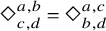Left: some collinearities between centres of points. Right: all centres belonging to an $(n_4)$ configuration.

Figure 20 Long description

A two-panel geometric diagram. The figure illustrates how the centers of the incircles introduced in Figure 19 give rise to a new incidence configuration. In the left panel, selected combinatorial square cells of the Poncelet grid are shown together with their incircles. The centers of these circles are marked by colored points. Some centers tangent to the same lines are connected by colored lines, revealing that they are collinear. The right panel displays the complete arrangement of three combinatorial types of incircles together with their centers. The centers lie on three families of conics and form the (n sub 4) configuration described in Theorem 3.6.

We extend our notation and use the symbols $\bigcirc ^{a,b}_{c,d}$ for the incircle and $\odot ^{a,b}_{c,d}$ for the incircle centre of a square cell . We now generate configurations from centres of incircles. For ease of notation we set ${}_{i}\odot _{k,l}:=\odot ^{i,i+l}_{i+k,i+k+l}$ .

Theorem 3.6. Let L be the lines supporting the sides of a Poncelet m-gon and let $a,b,c$ be three positive, distinct indices smaller than $m/2$ . Then the collection of centres

$$\begin{align*}\mathcal{P}:= \left\{ {}_{i}\!\odot_{a,b}\ \big\vert \ 1\leq i\leq m \right\}\cup \left\{ {}_{i}\!\odot_{b,c}\ \big\vert \ 1\leq i\leq m \right\}\cup \left\{ {}_{i}\!\odot_{c,a}\ \big\vert \ 1\leq i\leq m \right\} \end{align*}$$

are the points of a pre- $(n_4)$ configuration.

Figure 21

The full relation between incircle nets and the construction for $(n_4)$ configurations.

Figure 21 Long description

The figure extends the drawing of Figure 21. Here corresponding quadruples of incircles are connected by line segments. Each incircle center belongs to exactly four sich segment. The points together wich the segments form an (n sub 4) configuration. The figure visually summarises the two complementary constructions established in Theorems 3.1 and 3.6.

Proof. With everything we have already said, the proof is fairly easy. We have to show that each point is contained in 4 lines that contain 4 points each. Fix $a,b,c$ as well as i as in the Theorem. Since all points in $\mathcal {P}$ are defined in the same way, it suffices to show the existence of the four lines for one of the points $p=:{}_{i}\odot _{a,b}$ . It corresponds to the cell . Consider the points

$$\begin{align*}{}_{i-b}\odot_{a,b}=\odot^{{\color{black}i-b},{\color{red}i}}_{{\color{black}i-b+a},{\color{red}i+a}};\qquad {}_{i}\odot_{c,a}=\odot^{{\color{red}i},{\color{red}i+a}}_{{\color{black}i+c},{\color{black}i+a+c}};\qquad {}_{i-c}\odot_{c,a}=\odot^{{\color{black}i-c},{\color{black}i-c+a}}_{{\color{red}i},{\color{red}i+a}}. \end{align*}$$

Those indices marked in red show that each of the corresponding circles is tangent to the lines i and $i+a$ . Thus their centres and point p are four collinear points. All the points we considered are in the collection $\mathcal {P}$ given in the theorem. In exactly the same way it can be shown that there are three more four-point lines: one defined by the pair of lines $\{i,i+b\}$ , one defined by $\{i+a,i+a+b\}$ and one defined by $\{i+b,i+a+b\}$ .

3.3.3 Billiard geometry and local coordinate systems

Mathematics is the art of giving the same name to different things.

Poincaré

In this section, we take a different perspective and relate billiard trajectories in ellipses and their relationship to Poncelet polygons to our $\wedge $ and $\vee $ constructions. We first recall a few basic concepts. For a detailed exposition, see [Reference Tabachnikov56]. Consider an elliptic billiard table and draw the trajectory of a ball. The ball is reflected whenever it hits the cushion by the optical reflection law (so we do not do trickshots). Figure 22 shows an infinite and a closed trajectory. It turns out that all segments of a trajectory are tangent to a single conic, a caustic, that is confocal to the billiard table boundary. So if a trajectory returns to its initial starting conditions (position and direction), we actually create a Poncelet polygon. This relation between Poncelet chains and billiard trajectories can be exploited in various ways.

Figure 22

Billiard on an elliptic table. An open and a closed trajectory.

Figure 22 Long description

Two side-by-side panels each feature a green elliptical boundary representing a billiard table.In the left panel, an open trajectory is shown. A black line starts at a small white circle in the lower-left quadrant and reflects repeatedly off the outer green boundary. These reflections are dense and numerous, creating a thick band of lines that never repeat the same path. The lines are tangent to a smaller, invisible inner ellipse, known as a caustic, leaving the very center of the table empty.In the right panel, a closed trajectory is shown. A black line starts at a similar white circle in the lower-left quadrant but follows a much simpler, periodic path. The line reflects off the outer boundary only a few times before returning to its starting point, forming a distinct star-like geometric polygon. Like the first panel, this path also remains tangent to a central elliptical caustic region.

The concept of billiards on elliptic tables is tightly interwoven with our elaborations on Poncelet’s Porism and $(n_4)$ configurations. Our Theorem A states that if we start with an arbitrary Poncelet polygon P and construct $\wedge _{c}\cdot \vee _{b}\cdot \wedge _{a}\cdot \vee _{c}\cdot \wedge _{b}\cdot \vee _{a}(P)=P'$ we end up with P again. In a sense, this statement can be decomposed in two parts.

1. 1. The points $P'$ are on the same conic as the one that supports P, and

2. 2. on that conic they end up at the same position as the original points.

The billiard approach can be used to derive the second part relatively easily by introducing a certain distorted coordinate system that comes from the specific initial Poncelet polygon. In what follows we will sketch this line of reasoning.

We restrict ourselves to classes of confocal ellipses. We assume that the ellipses are equipped with a counterclockwise orientation. For the moment, we fix the two foci $f_1$ and $f_2$ , and only consider Poncelet m-gons whose inscribing and circumscribing ellipses have these focal points. Assume that the conic $\mathcal {X}$ to which the segments of the Poncelet polygon are tangent is given and fixed, and that the conic $\mathcal {C}$ on which the points lie is variable (but still with foci $f_1$ and $f_2$ ). The possible ellipses $\mathcal {C}$ form a one-parameter family.

Assume that an ordered pair of points $(P,Q)$ on $\mathcal {X}$ is given. The tangents at these points do have an intersection that uniquely defines a corresponding ellipse $\mathcal {C}$ . We equip this conic with a sign depending on the angle between P and Q as seen from the centre of the conic. The sign is positive if the angle is less than $\pi $ , zero if the angle is $0$ or $\pi $ , and negative otherwise. We consider another pair of points $(P',Q')$ to be equivalent to $(P,Q)$ if it defines the same signed conic $\mathcal {C}$ . We call an equivalence class $[P,Q]$ that arises that way a shift. We can define an addition on shifts by juxtaposition: $[P,Q]+[Q,R]=[P,R]$ . We can consider shifts as a kind of rotation along the conic by a certain amount (similar to rotations along a circle). However, the measurement is distorted by the specific geometry of the conic. Addition of shifts turns out to be commutative. This is a consequence of the incidence theorem sketched in Figure 23 on the right. All in all, the shifts around an ellipse form a commutative group similar to rotations on the boundary of a circle. The neutral element is shift $[P,P]$ and the inverse of $[P,Q]$ is $[Q,P]$ .

Figure 23

Shifts on an elliptic boundary. The left picture shows the same shift represented by two pairs of points. The picture on the right illustrates commutativity. We have two shifts $c=[P,Q]=[Q',R]$ and $d=[P,Q']=[Q,R]$ . It holds $c+d=[P,Q]+[Q,R]=[P,R]=[P,Q']+[Q',R]=d+c$ .

Figure 23 Long description

Two-panel geometric diagram showing shifts on elliptic boundaries. The left panel shows shifts with points P, Q, and P', Q'. The figure introduces the shift operation on two confocal ellipses. In the left panel, two billiard trajectories tangent to the same caustic define a constant shift c between corresponding vertices of different polygons. An inner blue and a confocal red conic is shown. Point P is on the inner conic. From there a tangent is draw that hits the outer conic and bounces back. After bouncing it again hots the inner conic in Q. This defines the shift operation. The Panel on the right introduces a third green confocal conic showing that if there is a shift c from P to Q and a shift d from Q to R then there is also a shift d from P to Q' followed by a shift c from Q' to R. Thus two shifts commute.

Shifts operate on the points of $\mathcal {X}$ . If c is a shift and $P\in \mathcal {X}$ , then there is a unique point $Q\in \mathcal {X}$ such that $[P,Q]=c$ . The operation of the shifts on P is defined by $[P,Q]\circ P=Q$ . If we fix a starting point $P_0$ on the conic $\mathcal {X}$ and a shift c, the sequence $P_{i+1}=c\circ P_i$ defines a Poncelet chain. It is completely determined by P and c. Since by Poncelet’s Porism the closing of the chain is not dependent on the starting point, the property of closing after m steps is entirely determined by c. Thus for a given m and $\mathcal {X}$ , a Poncelet m-gon with all vertices in cyclic order occurs only for one specific choice of c.

In [Reference Izmestiev33, Reference Levi and Tabachnikov39] it is proved that there is an isomorphism $\phi $ between the shifts on $\mathcal {X}$ and the half-open interval $[0,1)$ (with $\phi (c_1+c_2)=\phi (c_1)+\phi (c_2)\ \mathrm {mod} \ 1$ ). We can consider this isomorphism as a normalised measurement of distances along the conic. See [Reference Stachel53] for information about this measurement and for figures that illustrate the correspondence between shifts and $\wedge $ - $\vee $ operations.

Taking everything together, shifts can be represented in four different ways:

• • by ordered pairs $(P,Q)$ ,

• • as the corresponding signed conic $\mathcal {C}$ ,

• • as a number $0\leq c< 1$ ,

• • by a Poncelet chain, modulo a starting point.

Poncelet m-gons with points cyclically ordered arise if a shift subdivides $[0,1)$ into m equal parts. This happens for $\phi (c)=1/m$ . If appropriate, we may in the case of Poncelet polygons renormalise our measure again by multiplying it with m and calculate modulo m. Then the points of a Poncelet polygon appear at places $x+i$ for some integer i and some real number x.

Now we relate this point of view to our considerations about constructions and configurations from the previous sections. For that we have to relate shift measures of different confocal ellipses. Consider the following incidence Lemma whose geometric situation is depicted in Figure 24.

Figure 24

Left: Halving a shift can be represented by a transformation that maps one conic to the other. The intersection of the tangents is mapped to the halving point. Right: repeated occurrence of this situation in the $\wedge _{a}(L)$ operation.

Figure 24 Long description

Two panels showing geometric constructions of ellipses. The left figure introduces the geometric halving operation associated with billiard shifts. An inner black ellipse is shows together two points P and Q on it and tangents at these points. There intersection determines a blue ellipse confocal to the black one. Now w projective transformation tau is shown that maps the blue to the black conic. The image of the intersection of the tangents is mapped by tau to a point R. By construction the shifts P to R and R to Q are equal. The right panel shows how this construction can be used to construct a Poncelet 2 n gon from a Poncelet n gon. An inner black ellipse is shown with the points of a Poncelet polygon. since the shifts in a Poncelet n gon are all identical each of them can be halved this results in a Poncelet 2 n gon.

We will not prove this lemma here, since we only sketch the main lines of thought. A proof can be found implicitly in [Reference Izmestiev33, Reference Levi and Tabachnikov39]. The situation is relevant for our construction of $(n_4)$ configurations, and helps to relate the positions of the rings of lines and rings of points to each other. Consider Figure 24 on the right. It shows two rings of points in our construction of the main theorem together with the corresponding lines that connect them. The two rings lie on two conics $\mathcal {B}$ and $\mathcal {C}$ , and the lines are tangent to a conic $\mathcal {X}$ . We represent the lines by the respective touching points on $\mathcal {X}$ . By the Poncelet Grid Theorem, each ring of points forms a Poncelet m-gon. Without loss of generality, we may consider all three conics to be confocal. The points on $\mathcal {C}$ form a Poncelet m-gon that are generated by a shift c. Although the other rings of points lie on confocal conics, they are not generated by a uniform shift along these conics. However, by mapping them to the inner conic, we can relate them to a shift, as we will see next.

The situation repeatedly contains the geometric situation of Lemma 3.7. By the projective transformation induced by Lemma 3.7 we may represent the points of one of the outer rings by the mapped points on the inner ring on $\mathcal {X}$ . All potential points on $\mathcal {X}$ are generated by the iterated shift $c/2$ . Each ring of points is either mapped to the original points $x+i\cdot c$ , or to the points shifted by $1/2$ related to the shifts $x+i\cdot c+{1\over 2}$ .

Let us step back for a moment. The above considerations give us the possibility to represent all points and lines of all rings in an $m\#(a_1,b_1;a_2,b_2;\ldots ;a_k,b_k)$ construction by points on one Poncelet $2m$ -gon on a single conic. Let us assume that these points are labelled by $0.5, 1, 1.5, 2, 2.5, 3, 3.5, \ldots , m$ that represent their shifts referred to an initial point; we consider indices modulo m. Then, our operations $\vee _{a}$ and $\wedge _{b}$ for $1 \leq a,b<m/2$ may be expressed by a cyclic shift by $a/2$ , resp. ${(-b)/2}$ of these indices. The minus sign for the operation $\wedge _{b}$ occurs because we defined this operation by intersection of lines that are shifted clockwise (mathematically negative) by b index steps. The situation is depicted in Figure 25. After working out all the details in this approach, one can derive a conceptually very simple proof of the fact that the points in

$$\begin{align*}\wedge_{c}\cdot\vee_{b}\cdot \wedge_{a}\cdot\vee_{c}\cdot \wedge_{b}\cdot\vee_{a}(P) \end{align*}$$

are shifted identically to those of P.

Figure 25

Two examples of representing the operations $\vee _{a}$ and $\wedge _{b}$ by index shifts. The operation $\vee _{a}$ connects two points i and $i+a$ by a line that is tangent to the red conic in the dual Poncelet grid. Its touching point is mapped to a point $a\over 2$ on the central conic when the inner red conic is linearly blown up to match the outer one. Similarly $\wedge _{b}$ results in the point of intersection of two tangents. It lies on a certain conic of the Poncelet grid (not shown in the picture). Shrinking this conic down to the black conic maps this intersection to $-b\over 2$ .

Figure 25 Long description

The figure illustrates the geometric interpretation of the index arithmetic induced by the shift operation. An inner red and an outer black conic are shown. The outer conic carries the vertices of a Poncelet polygon, while the inner conic represents the associated billiard caustic. The labeled points show how shifts, half-shifts, and opposite shifts correspond to additions and divisions of the vertex indices modulo n. Tangent constructions identify the points representing the values a, b, a/2, and -b/2, demonstrating how the wedge and join operators become simple arithmetic operations on the cyclic index set. This geometric interpretation provides the foundation for the algebraic formulas developed in the subsequent theorems.

By our above considerations we represent each ring of points and lines by the points of one Poncelet $2m$ -gon generated by a shift $1\over 2m$ . Operations of the form $\wedge _{a}$ result in an index shift of $a\over 2$ on these points and operations of the form $\vee _{b}$ result in an index shift of $-b\over 2$ on these points. Thus, showing that the above sequence of operations results in the identity simply translates -- in the distorted metric of shifts -- to the simple equation

$$\begin{align*}{a\over 2} -{b\over 2} +{c\over 2} -{a\over 2} +{b\over 2} -{c\over 2}=0. \end{align*}$$

3.3.4 Pentagram map

We do not want to close this section without mentioning the relations of our results to the topic of pentagram maps. The pentagram map was introduced by R. Schwartz about 30 years ago, and it has been thoroughly studied since then. See [Reference Gekhtman, Shapiro, Tabachnikov and Vainshtein24, Reference Schwartz48, Reference Ovsienko, Schwartz and Tabachnikov40] for some initial literature. The pentagram map studies effects that arise when mapping the vertices of a polygon P to the intersections of diagonals of the polygon (similar to our $\wedge _{b}\cdot \vee _{a}(P)$ operations). Originally the map was only considered on the short diagonals of a polygon and it was later extended to more general cases.

Let us denote the short pentagram map by $T_2$ . It is constructed by connecting the vertices $p_i$ and $p_{i+2}$ of an m-gon and then intersecting consecutive diagonals. Similarly one defines the deeper-diagonal pentagram maps $T_k,\ k<m/2$ by connecting the vertices $p_i$ and $p_{i+k}$ . In our notation the map $T_k$ is represented by the operator $\wedge _{1}\cdot \vee _{k}$ .

The pentagram map commutes with projective transformations, and it descends to the moduli space of projective equivalence classes of polygons. Thus the polygons that arise are considered modulo projective transformations. The first (and slightly surprising) fact in this theory is that the map $T_2$ for the pentagon is the identity. In other words, the intersections of the diagonals of a pentagon are projectively equivalent to the original pentagon. This was already known to Clebsch [Reference Clebsch15]. In general, the resulting map is completely integrable in the sense of Liouville and, by now, it is one of the best known and most studied examples of a discrete integrable system. In particular, the pentagram map is intimately related with the recently emerged theory of cluster algebras.

With this notation, our Theorem B implies that, if applied to Poncelet polygons, these pentagram maps commute: $T_s \circ T_t = T_t \circ T_s$ , see Figure 26.

Figure 26

$T_2 \circ T_3=T_3 \circ T_2$ : both compositions send the red outer Poncelet octagon to the black inner one.

Figure 26 Long description

The figure illustrates the action of the pentagram map on a Poncelet octagon. Four successive polygonal configurations are superimposed: There is a red outer conic with the points of a Poncelet octagon on it. Star shaped figures are constructed by drawing lines that skip vertices of the octagon and intersecting adjacent resulting line. Eight green points are constructed by skipping one point. Eight blue points are obtained by skipping 2 points. The image illustrates how now skipping one point on the blue points and 2 points on the green points creates identical lines.

Let us mention that the pentagram map nicely interacts with Poncelet polygons. For example, recall that the pentagram map is completely integrable: a number of functions on the space of polygons are its integrals. It is proved in [Reference Schwarz51] that these integrals remain constant on the 1-parameter family of polygons, inscribed into one and circumscribed about another conic. As another example, it is proved in [Reference Izosimov35] that if a convex polygon is projectively equivalent to its pentagram image, then it is Poncelet.

3.3.5 The easier case of odd-gons

For the proof of our core Theorem A several essential ingredients had to be taken together: Poncelet grids, a continuous incidence theorem similar to Chasles’ Quadrilateral Theorem, an elaborate geometric construction, and careful bookkeeping of the labels and indices involved. Amazingly, if the number of points on the Poncelet polygons is odd, then a significantly simpler proof can be applied (actually, this is how we started). The deep reason for that is that for a Poncelet m-polygon P with odd m the result of the operation $(\wedge _{2}\cdot \vee _{1})(P)$ leads to a polygon that is projectively equivalent to P. This is not the case for even m. This projective equivalence provides a kind of shortcut in the argument. For that case we need the following strengthening of Theorem 2.1, a proof of which can be found in [Reference Levi and Tabachnikov39, Reference Schwartz49] (using different notation).

For the case in which the Poncelet polygon is supported by an ellipse $\mathcal {A}$ that is symmetric with respect to the coordinate axes we can express these projective transformations in a very simple way. The points $Q=(\wedge _{a}\cdot \vee _{1})(P)$ are the points of another Poncelet polygon supported by an ellipse $\mathcal {B}$ confocal to $\mathcal {A}$ . There are four natural projective transformations that map the ellipse $\mathcal {B}$ to $\mathcal {A}$ , by scaling the x and y coordinates. The four possibilities come from the different signs of the scaling in x and y direction. The projective transformation $\tau _a$ , whose existence is stated in the above theorem, that in addition maps the points set P to the point set Q, can be expressed as a diagonal $3\times 3$ matrix. For odd a this matrix has signature $(+,+,+)$ , and for even a the signature is $(-,-,+)$ .

If we want to overcome the fact that in this mapping the assignment is only setwise then we have to take a cyclic shift of indices into account. Let $\pi \in S_m$ be the permutation that cyclically shifts the points in $(1,\ldots , m)$ by one step. Then we get the following more precise formulation of Theorem 3.8.

From Theorem 3.8 this statement can be proved directly by careful bookkeeping of the indices. Let us denote the combined action of transformation and index shift as $F_a$ , where $(\wedge _{a}\cdot \vee _{1})(P)=F_a(P)$ . Notice that for shifts a and b, the operations $F_a$ and $F_b$ still commute.

Applying Theorem 3.9 to two different shifts a and b and using the fact that $F_a$ and $F_b$ commute we get:

$$\begin{align*}(\wedge_{a}\cdot\vee_{1})\cdot (\wedge_{b}\cdot\vee_{1})(P)=F_a(P)\cdot F_b(P)= F_b(P)\cdot F_a(P)=(\wedge_{b}\cdot\vee_{1})\cdot (\wedge_{a}\cdot\vee_{1})(P). \end{align*}$$

and hence

$$\begin{align*}(\wedge_{a}\cdot\vee_{1}\cdot \wedge_{b})(L)=(\wedge_{b}\cdot\vee_{1}\cdot \wedge_{a})(L). \end{align*}$$

Setting $P'= \wedge _{a}(L)$ (which implies $L= \vee _{a}(P')$ ) we get

$$\begin{align*}(\wedge_{a}\cdot\vee_{1}\cdot \wedge_{b}\cdot\vee_{a})(P')=(\wedge_{b}\cdot\vee_{1}\cdot \wedge_{a}\cdot\vee_{a})(P'). \end{align*}$$

Multiplying both sides by $\vee _{a}$ and cancelling leaves us with:

$$\begin{align*}(\vee_{1}\cdot \wedge_{b}\cdot\vee_{a})(P')=(\vee_{a}\cdot\wedge_{b}\cdot\vee_{1}\cdot)(P'). \end{align*}$$

Since we can bijectively go back and forth between Poncelet polygons by our $\wedge $ and $\vee $ operators, we can assume that $P'$ is an arbitrary Poncelet odd-gon. Also, a corresponding dual statement holds for lines L of a Poncelet odd-gon:

$$\begin{align*}(\wedge_{1}\cdot \vee_{b}\cdot\wedge_{a})(L)=(\wedge_{a}\cdot\vee_{b}\cdot\wedge_{1}\cdot)(L). \end{align*}$$

Taking these statements together we can derive Theorem A for odd m, as follows:

$$ \begin{align*} \vee_{a} \cdot \wedge_{b} \cdot \vee_{c}\ (P) &= \vee_{a} \cdot \wedge_{b} \cdot \vee_{c} \cdot \overbrace{\wedge_{1} \cdot \vee_{1}}^{\text{id}} \ (P)\\[1mm] &=\vee_{a} \cdot \underbrace{\wedge_{b} \cdot \vee_{c}\cdot \wedge_{1}}_{\wedge_{1} \cdot \vee_{c}\cdot \wedge_{b}} \cdot \vee_{1} (P)\\ &= \underbrace{\vee_{a} \cdot\wedge_{1} \cdot \vee_{c}}_{\vee_{c} \cdot\wedge_{1} \cdot \vee_{a}}\cdot \wedge_{b}\cdot \vee_{1} (P)\\ &=\vee_{c} \cdot\underbrace{\wedge_{1} \cdot \vee_{a}\cdot \wedge_{b}}_{\wedge_{b} \cdot \vee_{a}\cdot \wedge_{1}}\cdot \vee_{1} (P)\\ &=\vee_{c} \cdot\wedge_{b} \cdot \vee_{a}\cdot \underbrace{\wedge_{1} \cdot \vee_{1}}_{\text{id}}\ (P)\\ &=\vee_{c} \cdot \wedge_{b} \cdot \vee_{a}\ (P). \end{align*} $$

This is exactly the statement of Theorem A.

One might wonder why this approach cannot be applied in the case of Poncelet even-gons. The main obstacle is that the point sets $\wedge _{a}\cdot \vee _{1}(P)$ are not necessarily projectively equivalent to the points of P, depending on the parity of a. Hence, in that case, it is not easy to find the equivalent of the maps $F_a$ and $F_b$ . In a sense, our Lemma 3.3 presents an alternative way to obtain a commutative behaviour from which we could derive Theorem A.