2. The Abelian-Higgs model: self-dual vortices

The Abelian-Higgs model describes the minimal coupling between a $U(1)$ gauge field, which will be denoted by $A_\mu(x)=(A_0(x),A_1(x),A_2(x))$ and a complex scalar field, $\phi(x)=\phi_1(x)+i\phi_2(x)$ in a (1+2)-Minkowskian spacetime. After a suitable rescaling of the field and coordinates, the action can be written as

(2.1)\begin{equation} S[\phi,A]=\int d^3 x \left[ -\frac{1}{4} F_{\mu\nu}F^{\mu \nu} + \frac{1}{2} \overline{D_\mu \phi}\, D^\mu \phi -U(\phi,\overline{\phi}) \right] , \end{equation}

where the self-interaction potential term 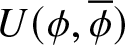$U(\phi,\overline{\phi})$ is given by

(2.2)\begin{equation} U(\phi,\overline{\phi}) = \frac{\lambda}{8} (\overline{\phi}\, \phi-1)^2 . \end{equation}

Here, $\overline{\phi}$ stands for complex conjugation of the scalar field and the covariant derivative is defined as $D_\mu \phi(x) = (\partial_\mu -i A_\mu(x))\phi(x)$, while the electromagnetic field tensor takes the standard form $F_{\mu\nu}(x)=\partial_\mu A_\nu(x) - \partial_\nu A_\mu(x)$. Throughout this work, we consider Minkowski space with the plus-minus metric convention $\eta_{\mu\nu}={\rm diag}(1,-1,-1),$ with $\mu,\nu=0,1,2$. We also adopt the Einstein summation convention over repeated indices. Greek indices refer to space–time coordinates, whereas Latin indices are reserved for purely spatial components. In the temporal gauge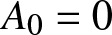 $A_0=0$, the second-order field equations governing the dynamics of the complex scalar field $\phi$ and the spatial components of the vector field $A_j$ take the form

(2.3)\begin{equation} \frac{1}{2}\partial_0^2 \phi - \frac{1}{2}D_jD_j\phi = - \frac{\partial U }{\partial \overline{\phi}} , \end{equation}

(2.4)\begin{equation} \partial_0^2 A_j - \partial_k F_{kj} = - \frac{i}{2} \Big[ \overline{\phi} \, D_j \phi - \overline{D_j \phi} \,\phi \Big] . \end{equation}

Equations (2.3) and (2.4) must be supplemented by the Gauss law

(2.5)\begin{equation} \partial_{0i}A_i = - \frac{i}{2} \Big[ \overline{\phi} \, \partial_0 \phi - \overline{\partial_0 \phi} \,\phi \Big] , \end{equation}

which is automatically satisfied by static solutions.

Vortices are topological defects whose energy density

(2.6)\begin{equation} \mathcal{E}[\phi,A] = \frac{1}{2} \partial_0 A_i \partial_0 A_i + \frac{1}{2} \overline{\partial_0 \phi} \partial_0 \phi + \frac{1}{2} F_{12}^2 + \frac{1}{2} \overline{D_i \phi} \, D_i \phi + \frac{\lambda}{8} (\overline{\phi} \phi -1)^2 \end{equation}

is localized around a point in the plane, which is naturally identified as the vortex centre. These configurations possess nontrivial topological properties that ensure their stability under perturbations. Vortex solutions arise as static solutions of the field equations (2.3) and (2.4) subject to the requirement that the total energy

(2.7)\begin{equation} E[\phi,A] = \int_{\mathbb{R}^2} dx_1 dx_2 \, \mathcal{E}[\phi,A] \end{equation}

remains finite. This condition imposes specific asymptotic boundary conditions on the fields at spatial infinity $S^\infty$. In particular, the scalar field must approach the vacuum configuration of the potential, which can be written as

(2.8)\begin{equation} \phi\Big|_{S^\infty} = e^{i n \theta} \, , \end{equation}

while the gauge field asymptotically approaches a pure gauge configuration

(2.9)\begin{equation} (A_1,A_2)\Big|_{S^\infty} = \left(-i e^{-in\theta} \partial_1 e^{in\theta},-ie^{-in\theta} \partial_2 e^{in\theta} \right) \, , \end{equation}

where $n\in \mathbb{Z}$. In Equations (2.8) and (2.9), we have introduced the angular variable $\theta$, which arises from the use of polar coordinates in the spatial plane, $x_1=r\cos\theta$ and $x_2=r \sin \theta$. Configurations characterized by different winding numbers $n$ in (2.8) belong to distinct topological sectors and are therefore classified by the elements of the additive group $\mathbb{Z}$. As a consequence, the magnetic flux carried by the vortices is quantized

\begin{equation*} \Phi = \frac{1}{2\pi} = \int_{\mathbb{R}^2} d^2 x F_{12} = n \in \mathbb{Z} \, . \end{equation*}

In this work, we restrict our attention to self-dual vortices, which arise when the coupling constant satisfies $\lambda = 1$ in the potential term (2.2). In this regime, the Bogomolny procedure can be applied to the energy functional (2.7) for static configurations, allowing it to be rewritten as the sum of two positive-definite contributions plus a term proportional to the topological charge

\begin{equation*} E[\phi,A] = \frac{1}{2} \int_{\mathbb{R}^2} \Big[ \Big(F_{12}\pm \frac{1}{2} (\overline{\phi} \phi -1) \Big)^2 + \Big| D_1\phi \pm i D_2\phi \Big|^2 \Big] \pm n\, \pi \, . \end{equation*}

As a consequence, the energy is bounded from below by the corresponding topological charge. Field configurations that saturate this bound satisfy a system of first-order differential equations, namely

(2.10)\begin{equation} F_{12}\pm \frac{1}{2} (\overline{\phi} \phi -1) = 0,\quad D_1\phi \pm i D_2\phi = 0 \, , \end{equation}

which are usually referred to as Bogomolny (self-duality) equations. Static rotationally invariant $n$-vortex solutions can be found by imposing the radial gauge condition $A_r=0$ and the ansatz

(2.11)\begin{equation} \phi(r,\theta) = f_n(r) e^{in\theta},\quad r A_\theta(r,\theta) = n \beta_n(r) \, , \end{equation}

where we adopt the convention $A_1=A_r \cos \theta - A_\theta \sin \theta$ and $A_2=A_r \sin \theta + A_\theta \cos \theta$. Substituting (2.11) into (2.10) implies that the radial profile functions $f_n(r)$ and $\beta_n(r)$ satisfy the differential equations

(2.12)\begin{equation} \frac{d f_n}{dr} = \pm \frac{n}{r} f_n(r) [1-\beta_n(r)],\quad \frac{d \beta_n}{dr} = \pm \frac{r}{2n} [1-f_n^2 ]. \end{equation}

Regularity of the solutions at the origin imposes the following conditions for the profile functions

\begin{equation*} f_n(0) = 0\quad \mbox{and}\quad \beta_n(0)=0 . \end{equation*}

It can be shown by using (2.12) that the power expansion of the $n$-vortex solutions around $r=0$ has the form

(2.13)\begin{equation} f_n(r) = r^n \Big( d_n - \frac{d_n}{8} r^2 + \dots \Big) ,\quad \beta_n(r) = r^2 \Big( \frac{1}{2n} - \frac{d_n^2}{4n(n+1)} r^{2n} + \dots \Big) , \end{equation}

where $d_n$ are real constants that depend on the topological charge $n$ of the vortex configuration and must be determined numerically. For the 1-vortex ( $n=1$), one finds $d_1 \approx 0.602941$. On the other hand, the asymptotic conditions for these solutions are

(2.14)\begin{equation} \lim_{r\rightarrow \infty} f_n(r)= 1 ,\quad \lim_{r\rightarrow \infty} \beta_n(r) = 1. \end{equation}

For intermediate values of $r$, Equations (2.12) must be solved numerically. The radial structure of the vortex solution can be conveniently characterized in terms of the scalar field modulus $f_n(r)$, the gauge field function $\beta_n(r)$ and the corresponding energy density $\mathcal{E}_n(r)=\mathcal{E}[f_n(r),\beta_n(r)]$ obtained from (2.6) using the ansatz (2.11). The profiles of these quantities as functions of the radial distance from the vortex centre are displayed in Figure 1 for different values of the topological charge $n$.

Figure 1.

Radial profiles of the scalar field modulus $f_n(r)$ (left), the function $\beta_n(r)$ determining the vector field (middle) and the energy density $\mathcal{E}_n(r)$ (right), plotted as functions of the radial distance from the vortex centre.

It is worth noting that the energy density attains its maximum at $r=0$ for the single-vortex configuration. In contrast, for vortices with higher vorticity, the energy density no longer peaks at the origin; instead, it forms a ring of maximal energy density located at a finite distance from the vortex centre.

3. Derrick-type fluctuations of self-dual vortices

In this section, we analyse the Derrick-type vibrational modes of vortex solutions. These modes preserve the same angular structure as the background vortex configuration. In other words, the perturbations respect the angular dependence of the original solution. In order to simplify the notation and make the analysis more transparent, we introduce a convenient notation for the solutions. The scalar and vector field profiles of a static rotationally invariant $n$-vortex will be, respectively, denoted by

\begin{equation*} \psi(\vec{x};n)=\psi_1(\vec{x};n) + i \, \psi_2(\vec{x};n) ,\quad V(\vec{x};n)=(V_1(\vec{x};n),\quad V_2(\vec{x};n)) \mbox{with} \vec{x}=(x_1,x_2) , \end{equation*}

which will be assembled into a four-component real column $\Psi(r,\theta) \in {\cal C}^\infty(\mathbb{R}^2) \otimes \mathbb{R}^4$ in the form

(3.1)\begin{equation} \Psi(r,\theta)=\left(\begin{array}{c} V_1(\vec{x};n) \\ V_2(\vec{x};n) \\ \psi_1(\vec{x};n) \\ \psi_2(\vec{x};n) \end{array} \right) = \left(\begin{array}{c}- \frac{n\beta_n(r)}{r} \sin \theta \\ \frac{n\beta_n(r)}{r} \cos \theta \\ f_n(r) \cos (n\theta) \\ f_n(r) \sin (n\theta) \end{array} \right). \end{equation}

In general, a perturbed $n$-vortex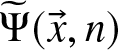 $\widetilde{\Psi}(\vec{x},n)$ can be written in the form

(3.2)\begin{equation} \widetilde{\Psi}(\vec{x},n) = \Psi(\vec{x},n) + \epsilon\, \xi(\vec{x})=\left(\begin{array}{c} V_1(\vec{x};n) \\ V_2(\vec{x};n) \\ \psi_1(\vec{x};n) \\ \psi_2(\vec{x};n)\end{array} \right) + \epsilon\, \left(\begin{array}{c} a_1(\vec{x}) \\ a_2(\vec{x}) \\ \varphi_1(\vec{x}) \\ \varphi_2(\vec{x}) \end{array} \right), \end{equation}

where

\begin{equation*} \xi(\vec{x})=\left( \begin{array}{c c c c}a_1(\vec{x}) & a_2(\vec{x}) & \varphi_1(\vec{x}) & \varphi_2(\vec{x}) \end{array} \right)^t , \end{equation*}

denotes the fluctuation column, which describes small fluctuations of the scalar and gauge fields around the static vortex solution 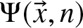$\Psi(\vec{x},n)$, and $\epsilon$ is the amplitude of the perturbation. To discard pure (non-physical) gauge fluctuations, the so-called background gauge

(3.3)\begin{equation} \partial_1 a_1( \vec{x}) + \partial_2 a_2( \vec{x}) - (\,\psi_1( \vec{x})\, \varphi_2( \vec{x})-\psi_2( \vec{x})\,\varphi_1( \vec{x})\,)=0 \end{equation}

is imposed as the gauge-fixing condition on the fluctuation modes. With this setup, the normal modes of an $n$-vortex solution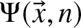 $\Psi(\vec{x},n)$ are determined by the spectral problem

(3.4)\begin{equation} {\cal H}^+ \xi_\nu(\vec{x}) =\omega_\nu^2 \, \xi_\nu(\vec{x}) , \end{equation}

where $\nu$ labels eigenfunctions in both the discrete and continuous spectra used to enumerate the eigenfunctions and eigenvalues, and ${\cal H}^+$ is the second-order small fluctuation operator

(3.5)\begin{equation} {\cal H}^+= \left( \begin{array}{cccc} \!-\Delta + |\psi|^2 & 0 & \!-2 \widetilde{D}_1 \psi_2 & 2 \widetilde{D}_1 \psi_1 \\ \!0 & -\Delta +|\psi|^2 & \!-2 \widetilde{D}_2 \psi_2 & 2 \widetilde{D}_2 \psi_1 \\ \!-2 \widetilde{D}_1 \psi_2 & \!-2 \widetilde{D}_2\psi_2 & \!-\Delta + \frac{3\lambda}{2} \psi_1^2 + (1+\frac{\lambda}{2})\psi_2^2 \!-\frac{\lambda}{2} \!+V_kV_k & \!-2 V_k \partial_k + (\lambda\!-\!1)\psi_1\psi_2\\ \!2\widetilde{D}_1\psi_1 & 2 \widetilde{D}_2 \psi_1 & 2V_k \partial_k + (\lambda\!-\!1)\psi_1\psi_2 & -\Delta + (1+\frac{\lambda}{2})\psi_1^2 +\frac{3\lambda}{2} \psi_2^2 \!-\!\frac{\lambda}{2} + V_kV_k \end{array} \right) \end{equation}

where $\widetilde{D}_i\psi_j = \partial_i\psi_j+\epsilon^{ik} V_i \psi_k$. The Sturm–Liouville eigenvalue problem (3.4) is obtained by linearizing the field equations (in the background gauge) around the vortices, see [Reference Alonso-Izquierdo, Garcia-Fuertes and Mateos-Guilarte6]. The fluctuation eigenfunctions $\xi(\vec{x})$ in general belong to a rigged Hilbert space, such that there exist square-integrable eigenfunctions $\xi_\nu(\vec{x})\in L^2(\mathbb{R}^2)\otimes \mathbb{R}^4$ associated with the discrete spectrum, for which the norm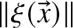 $\|\xi(\vec{x})\|$ is bounded:

(3.6)\begin{equation} \|\xi(\vec{x})\|^2 = \int_{\mathbb{R}^2} d^2x \Big[ (a_1(\vec{x}))^2 + (a_2(\vec{x}))^2 + (\varphi_1(\vec{x}))^2 + (\varphi_2(\vec{x}))^2 \Big] \lt +\infty \, , \end{equation}

together with non-normalizable (scattering) eigenfunctions $\xi_\nu(\vec{x})$ with $\nu$ ranging in a dense set.

Following the previous description of the Derrick-type modes, we adopt the ansatz

(3.7)\begin{equation} \xi_\nu(\vec{x},n) = \left( \begin{array}{c} v_n(r) \, \sin \theta \\ - v_n(r) \,\cos \theta \\ u_n(r) \, \cos(n\theta) \\ u_n(r) \, \sin(n\theta) \end{array} \right), \end{equation}

which preserves the angular symmetry of the background vortex configuration and where the functions $v_n(r)$ and $u_n(r)$ depend on the vorticity of the solutions. Substituting this expression into the spectral problem (3.4) leads to a reduced eigenvalue problem for the radial profiles $v_n(r)$ and $u_n(r)$. In this way, the original problem simplifies to

(3.8)\begin{equation} {\cal H}^+_R \zeta_\nu (x) = \omega_\nu^2 \zeta_\nu(x) \, , \end{equation}

where the radial functions comprise the column $\zeta_\nu (r)= (v_n(r),u_n(r) )^t$ and the operator ${\cal H}^+_R$ is given by

(3.9)\begin{equation} {\cal H}^+_R = \left( \begin{array}{cc} - \frac{d^2}{dr^2} - \frac{1}{r} \frac{d}{dr} + \frac{1}{r^2} + f_n^2(r) & \frac{2n}{r} (1-\beta_n(r)) f_n(r) \\ \frac{2n}{r} (1-\beta_n(r)) f_n(r) & - \frac{d^2}{dr^2}- \frac{1}{r} \frac{d}{dr} + \frac{n^2 (1-\beta_n(r))^2}{r^2} + \frac{3}{2} f_n^2(r) - \frac{1}{2} \end{array} \right). \end{equation}

In this work, we focus on the dynamics of excited single-vortex configurations. In particular, we are interested in identifying the vibrational modes arising from the spectral problem (3.9) for the case $n=1$. In this situation, the spectrum contains a single bound eigenstate with eigenvalue

\begin{equation*} \omega^2= 0.77741. \end{equation*}

This shows that the 1-vortex configuration admits only one internal vibrational mode, corresponding to an excitation that modifies the spatial extent of the vortex according to the eigenfunction $\xi(\vec{x},1) e^{i\omega t}$ at first-order. The period of this oscillatory motion is therefore given by $T=\frac{2\pi}{\omega} \approx 8.0822$. Figure 2 illustrates the time evolution of an excited 1-vortex undergoing this vibrational motion. The figure displays five snapshots of the energy density of the configuration: the first corresponds to an initial time, while the subsequent frames are taken at time intervals of $T/4$ (in dimensionless units). This sequence clearly illustrates the periodic expansion and contraction of the vortex core associated with the Derrick-type excitation. Correspondingly, the peak of the energy density at the vortex centre exhibits an oscillatory behaviour in time.

Figure 2.

Snapshots of the energy density of an excited 1-vortex. The five frames correspond to times separated by $T/4$, showing the periodic expansion and contraction of the vortex core associated with the Derrick vibrational mode.

To analyse the oscillatory pattern of the energy density discussed above, we first need to determine the behaviour of the vibrational modes at the 1-vortex centre. This behaviour can be analysed using the Frobenius method applied to the differential equations derived from (3.8). This procedure leads to expressions of the form

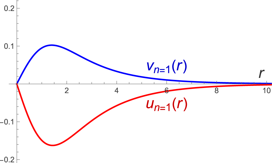
(3.10)\begin{equation} v_{n=1}(r) \approx v_0 \, r, u_{n=1}(r) \approx u_0 \, r \end{equation}

for the radial profiles in the limit $r\approx 0$ where $v_0$ and $u_0$ must be determined numerically. In particular, $v_0\approx 0.129152$ and $u_0 \approx -0.200432$. The global radial profiles of the normalized Derrick vibrational mode are shown in Figure 3, where the behaviour described above can be clearly observed.

Figure 3.

Radial profiles of $u_n(r)$ and $v_n(r)$ for the Derrick vibrational mode of the 1-vortex obtained numerically from the reduced spectral problem (3.8).

The expressions (3.10) can be used to determine how the peak of the 1-vortex energy density evolves when the configuration is subjected to such a Derrick-type excitation. To this end, we substitute the expressions (2.13), which describe the behaviour of the scalar and gauge field radial profiles near $r\approx 0$, together with the corresponding expressions (3.10) for the functions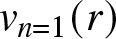 $v_{n=1}(r)$ and $u_{n=1}(r)$ that characterize the behaviour of the Derrick-type vibrational mode in the vortex core, into the linearly perturbed vortex configuration (3.2). Substituting these expansions into the energy density (2.6), one can evaluate the time dependence of the energy density at the vortex centre by taking the limit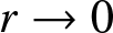 $r\rightarrow 0$. In this way, we obtain an explicit expression describing the temporal evolution of the peak of the vortex energy density, which is given by

(3.11)\begin{equation} {\cal E}_{\rm max}(t) = 0.613538 - 0.370849 \, \epsilon \sin (0.881709 \, t) + 0.0735335 \, \epsilon^2 \sin^2 (0.881709 \, t) \, . \end{equation}

In this expression, $\epsilon$ denotes the amplitude of the perturbation appearing in (3.2), assuming that the eigenfunction $\xi(\vec{x})$ is normalized over the plane, that is,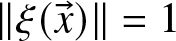 $\|\xi(\vec{x})\|=1$. In the derivation of (3.11), only the linear contribution of the perturbed vortex solution has been taken into account. Even at this order, however, the resulting expression for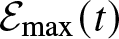 ${\cal E}_{\rm max}(t)$ contains a quadratic dependence on the excitation amplitude $\epsilon$. It is important to note that this quadratic term only modifies the average value of the maximum energy density

\begin{equation*} \overline{\cal E}_{\rm max} = 0.613538 +0.0367667 \epsilon^2. \end{equation*}

By contrast, the quantity relevant for the present work, namely the oscillation amplitude, remains unaffected by this contribution. This can be verified by observing that the critical points of the time-dependent function 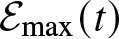${\cal E}_{\rm max}(t) $ occur at

\begin{equation*} t_1(k) \approx 1.78154 + 3.56307 \, k\quad \mbox{and}\quad t_2(k) \approx \frac{1}{0.881709}\arcsin \frac{0.326981}{0.12967 \epsilon} + 3.56307 \, k \end{equation*}

where $k\in \mathbb{Z}$. The second set of critical points $t_2(k)$ appears only when the perturbation amplitude satisfies $\epsilon \geq 2.52164$. Such a value corresponds to a highly excited vortex configuration, which is far from the linear regime and is unlikely to occur in realistic situations. For this reason, in the following analysis, we restrict our attention to smaller excitation amplitudes. In this case, the oscillatory behaviour of the peak energy density can be characterized by considering the difference between the maximum and minimum values reached during one oscillation cycle. Using the expressions for the maxima and the minima occurring at the times $t_1(k)$, one obtains

(3.12)\begin{equation} \Delta {\cal E}_{\rm max} \approx 0.741699 \, \epsilon. \end{equation}

This relation provides a simple and efficient way to estimate the amplitude of the vortex excitation directly from the variation of the peak energy density. Indeed, we will use it for extracting the final excitation amplitude in our numerical simulations of vortex scattering processes.

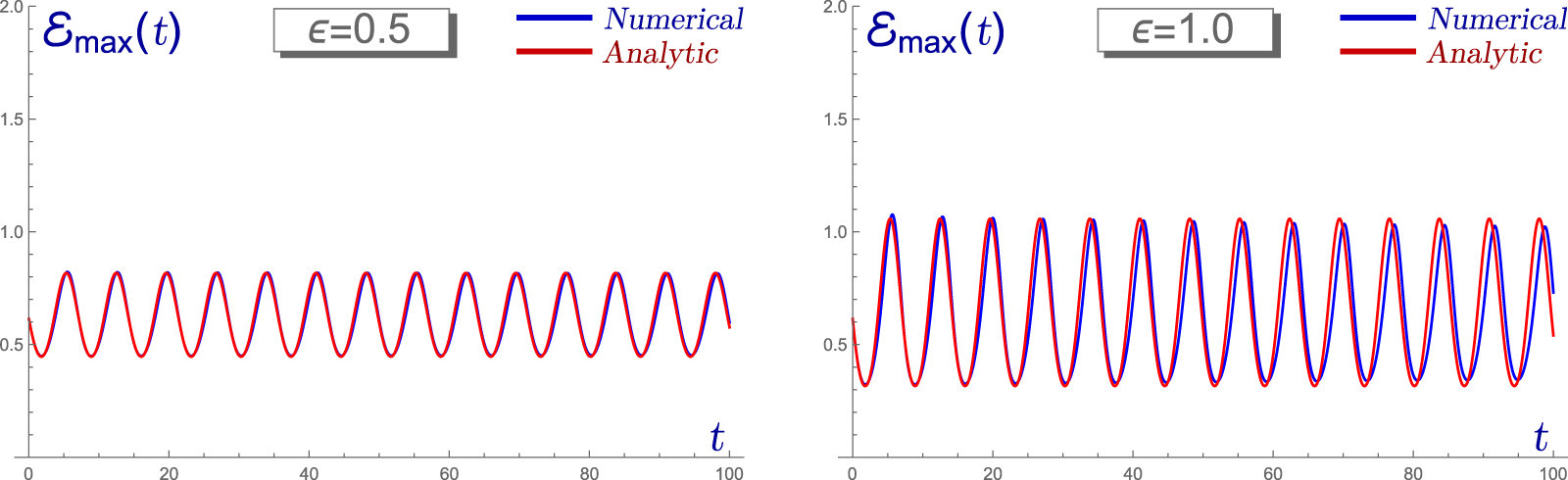
Strictly speaking, a fully consistent perturbative treatment would also require the inclusion of quadratic corrections in the perturbed vortex solution itself, in order to determine whether additional higher-order contributions to (3.11) may arise. Nevertheless, direct numerical comparison shows that the effect of such corrections is extremely small, even for moderately large excitation amplitudes. To validate (3.11), we perform a series of numerical experiments for different excitation amplitudes. In particular, in Figure 4, we consider initially excited 1-vortex configurations centred at the origin with amplitudes 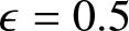$\epsilon=0.5$ and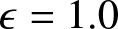 $\epsilon=1.0$. We display the time evolution of the maximum energy density of the excited vortex (blue curve) together with the analytical prediction provided by expression (3.11) (red curve). The excellent agreement between the two curves confirms that expression (3.11) can be reliably used to determine the excitation amplitude of the vortex. Naturally, nonlinear effects become progressively more important as the excitation amplitude increases. In particular, for $\epsilon=1.0$, one can already observe a slow decay of the oscillation amplitude in time, associated with radiation effects. This phenomenon has been analysed in detail in [Reference Alonso-Izquierdo, Blanco-Pillado, Miguélez-Caballero, Navarro-Obregón and Queiruga4].

Figure 4.

Time evolution of the peak energy density of an excited 1-vortex. Numerical results (blue) are compared with the analytical prediction given by expression (3.11) (red). The panels correspond to excitation amplitudes $\epsilon=0.5$ (left) and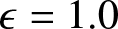 $\epsilon=1.0$ (right).

In this work, we are interested in studying the dynamics of excited 1-vortices, and in particular, the collision of two of them. We note that the theory defined in (2.1) is Lorentz invariant. Consequently, the static vortex solutions $(V_0,V_1,V_2,\psi)$ constructed in the previous sections can be transformed into travelling vortex solutions $(V_0^{(v)},V_1^{(v)},V_2^{(v)},\psi^{(v)})$ with velocity $v$ by applying a Lorentz boost in the $x_1$-direction, i.e.,

\begin{align*} \psi^{(v)}(x_i,t) & = \psi (x_i',t') \, , \\ V_0^{(v)}(x_i,t) &= \frac{V_0(x_i',t')}{\sqrt{1-v^2}} - \frac{v \, V_1(x_i',t')}{\sqrt{1-v^2}} \, ,\\ V_1^{(v)}(x_i,t) &= - \frac{v V_0(x_i',t')}{\sqrt{1-v^2}} + \frac{V_1(x_i',t')}{\sqrt{1-v^2}} \, ,\\ V_2^{(v)}(x_i,t) & = V_2 (x_i',t') \, , \end{align*}

where

\begin{equation*} x_1'= \frac{x_1-v t}{\sqrt{1-v^2}} , x_2'=x_2\quad \mbox{and}\quad t'= \frac{t-vx_1}{\sqrt{1-v^2}} \, . \end{equation*}

When a vortex moves with velocity $v$, these relativistic effects must be taken into account. Following the same analytical reasoning used in the static case, but adapted to the boosted configuration, one arrives at the expression

\begin{equation*} {\cal E}_{\rm max}^{(v)}(t) = {\cal E}_{\rm max}(t) + [-0.275519 + 0.088560 \epsilon \sin (0.881709 t) - 0.011746 \epsilon^2 \sin^2 (0.881709 t) ] v^2, \end{equation*}

which depends on the velocity $v$ of the travelling vortex. The motion of the vortex leads to the transverse Doppler effect, which modifies the expression (3.12) that describes the oscillatory behaviour of the energy-density peak for vortices at rest, which now reads

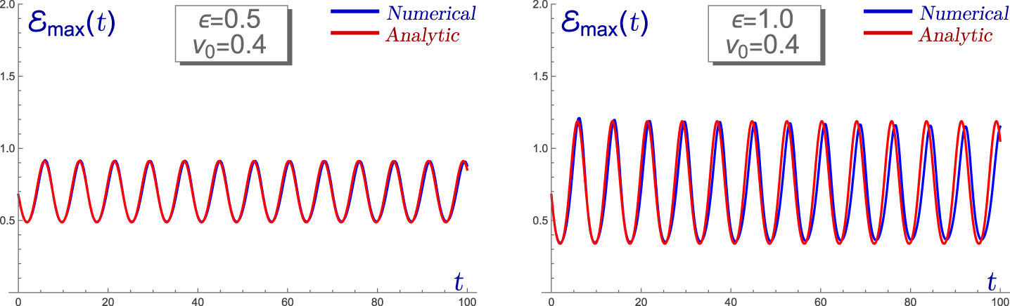
(3.13)\begin{equation} \Delta {\cal E}_{\rm max}^{(v)} \approx \frac{(0.741699 -0.177121 v^2)\, \epsilon}{1-v^2}. \end{equation}

As before, we illustrate the temporal evolution of the peak of the energy density, located at the vortex centre, when the vortex moves with a constant velocity (in this case 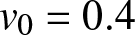$v_0=0.4$), see Figure 5. The numerical result is compared with the analytical prediction. The comparison shows an excellent agreement between the two curves: the blue curve corresponds to the numerical simulation, while the red curve represents the analytical prediction. This confirms that the generalized expression (3.13) accurately describes the oscillatory behaviour of the energy-density peak for moving vortices.

Figure 5.

Time evolution of the peak energy density of a moving excited 1-vortex. Numerical simulation (blue curve) is compared with the analytical prediction (red curve) for a vortex moving with velocity 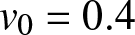$v_0=0.4$.

Note that the numerical coefficients appearing in (3.12) and (3.13) arise because neither the vortex profiles nor the vibrational eigenfunctions admit closed analytical expressions. Their behaviour near the vortex centre must therefore be determined numerically. In this sense, these equations combine analytical derivation with numerical input.

4. Scattering of excited self-dual vortices

In this section, we analyse the dynamics of excited vortices to understand how the motion of these topological defects is affected by internal oscillations of the vortices associated with a Derrick-type vibrational mode. In particular, we are interested in determining how such excitations influence the dynamics of vortex–vortex collisions. In this context, two main mechanisms are expected to play an important role in the dynamics: the resonant energy transfer mechanism and the mode-driven force between vortices.

The first of these effects is well-known and was originally identified in one-dimensional field theories, namely in 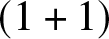$(1+1)$-dimensional Minkowski space, [Reference Campbell, Schonfeld and Wingate16, Reference Goodman and Haberman20, Reference Goodman and Haberman21, Reference Manton, Oleś, Romańczukiewicz and Wereszczyński29, Reference Sugiyama39]. A paradigmatic example is provided by kink–antikink collisions in the $\phi^4$ model. In this system, during the collision process, a redistribution of energy takes place between the translational kinetic energy of the solitons and their internal vibrational modes. As a consequence, the outgoing kinetic energy after the first impact may become insufficient for the defects to escape from each other due to their mutual attraction. In such situations, the kink and antikink undergo a sequence of multiple collisions until the energy is transferred back to the translational mode, eventually allowing the defects to separate. This mechanism leads to the well-known fractal structures observed in the scattering diagrams that relate the final escape velocity of the kinks to their initial collision velocity. These fractal patterns appear even when the kink and antikink collide without being initially excited through their internal shape mode. When the defects are initially excited, the complexity of these structures becomes even more pronounced [Reference Alonso-Izquierdo, Nieto and Queiroga-Nunes11, Reference Izquierdo, Queiroga-Nunes and Nieto25].

The situation is qualitatively different in the case of self-dual vortices in the Abelian-Higgs model. In this system, unperturbed self-dual vortices do not experience intersolitonic forces, which allows the role of the resonant energy transfer mechanism to be investigated in a more isolated and controlled way. In particular, the absence of static forces between vortices makes it possible to analyse more clearly how internal excitations influence the dynamics of vortex scattering.

As a reference, we first recall the well-known scattering process of two unexcited 1-vortices approaching each other with low initial velocity. In this case, two vortices initially moving along the $x_1$-axis collide at the origin, forming a transient 2-vortex configuration, and subsequently separate along the $x_2$-axis with the same speed. This process corresponds to the characteristic $90^\circ$-scattering of BPS vortices, illustrated in Figure 6.

Figure 6.

Snapshots of the energy density of the scattering between two unexcited 1-vortices at low collision velocity. Two vortices approaching along the $x_1$-axis collide at the origin and subsequently separate along the $x_2$-axis with the same speed.

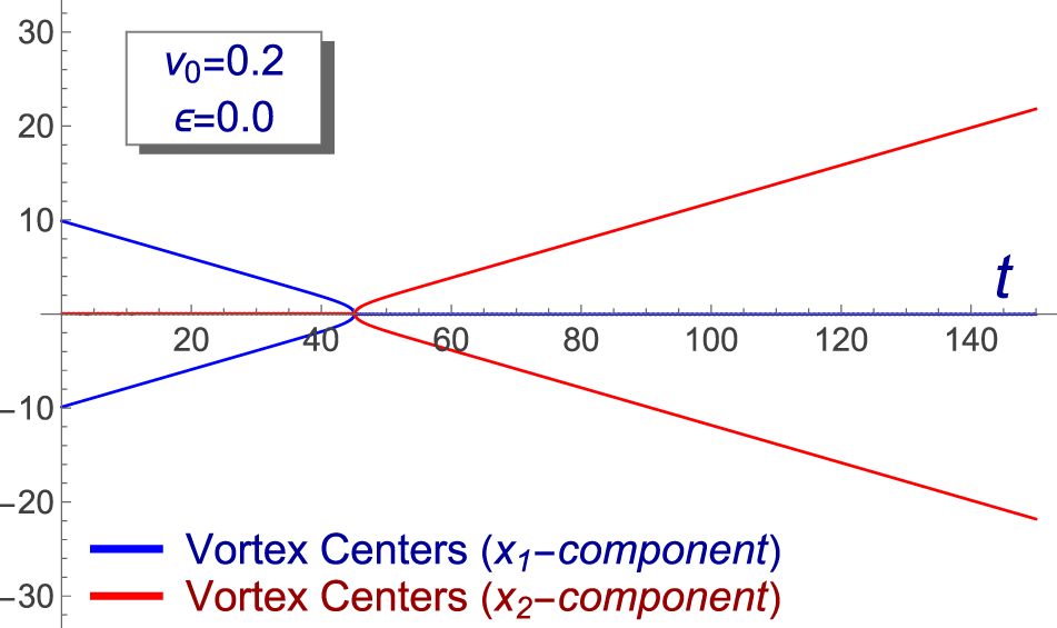
The scattering process described above can be illustrated more clearly by examining the trajectories of the vortex centres, as shown in Figure 7. In this figure, Cartesian coordinates of the vortex centres are plotted as functions of time. The blue curve represents the $x_1$-component of the position, while the red curve corresponds to the $x_2$-component. Before the collision, the vortices move along the $x_1$-axis. Consequently, the $x_2$-component of their positions remains zero, as reflected by the red curve remaining close to zero during this stage of the evolution. After the collision, however, the vortices separate along the $x_2$-axis. As a result, the $x_1$-component of their positions becomes zero, while the $x_2$-component evolves in time.

Figure 7.

Coordinates of the vortex centres as functions of time for the scattering of two unexcited vortices with initial velocity 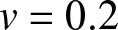$v=0.2$. The blue and red curves correspond to the $x_1$- and $x_2$-components of the positions, illustrating the characteristic $90^\circ$ vortex scattering.

To investigate the role of resonant energy transfer in vortex collisions, we perform a systematic scan over the initial collision velocity for the scattering of two 1-vortices. The scattering diagrams for the final velocities and excitation amplitudes are constructed using a default resolution of $\Delta v_0=0.001$. In regions where narrow resonant windows appear, the resolution is further refined down to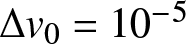 $\Delta v_0=10^{-5}$ in order to accurately resolve the underlying fine structure. The numerical simulations carried out in this work closely follow the framework developed in [Reference Krusch, Rees and Winyard27]. In particular, we adopt the same damping procedure, time-evolution scheme and natural boundary conditions described respectively in Section IV and Appendix B of that reference. The field equations in Lorenz gauge are discretized using fourth-order finite differences in space together with a second-order accurate time integration scheme. The vortices are initially placed symmetrically along the $x_1$-axis at positions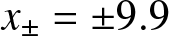 $x_\pm=\pm 9.9$. Initial configurations are generated by applying Lorentz boosts to static vortex solutions and combining them through the standard Abrikosov ansatz for well-separated vortices [Reference Abrikosov1],

\begin{equation*} \phi =\psi^{(v_0)}(x_1-x_-,x_2,t)\cdot \psi^{(-v_0)}(x_1-x_+,x_2,t) ,\ A_\mu= V_\mu^{(v_0)}(x_1-x_-,x_2,t) + V_\mu^{(-v_0)}(x_1-x_+,x_2,t). \end{equation*}

Simulations are performed on the square domain $[-30,30]\times[-30,30]$ with spatial resolution $\Delta x=\Delta y=0.15$. During the evolution, we monitor both the vortex trajectories and the energy density at the vortex cores. From these data, we extract the final velocities of the outgoing vortices together with their final excitation amplitudes using (3.13). One of the main advantages of this formula is that it provides a simple, robust and computationally efficient method for estimating the final excitation amplitudes. Unlike the approach employed in [Reference Krusch, Rees and Winyard27], where the amplitudes were inferred from the time evolution of the total potential energy (requiring the computation and spatial integration of the energy density over the entire grid at every time step), (3.13) only relies on local information near the vortex cores. More precisely, it is sufficient to monitor the maxima and minima of the energy density in the vicinity of each vortex centre during the evolution. This significantly reduces the computational cost and, moreover, allows each vortex to be analysed independently, even in situations where the outgoing vortices oscillate with different amplitudes or relative phases.

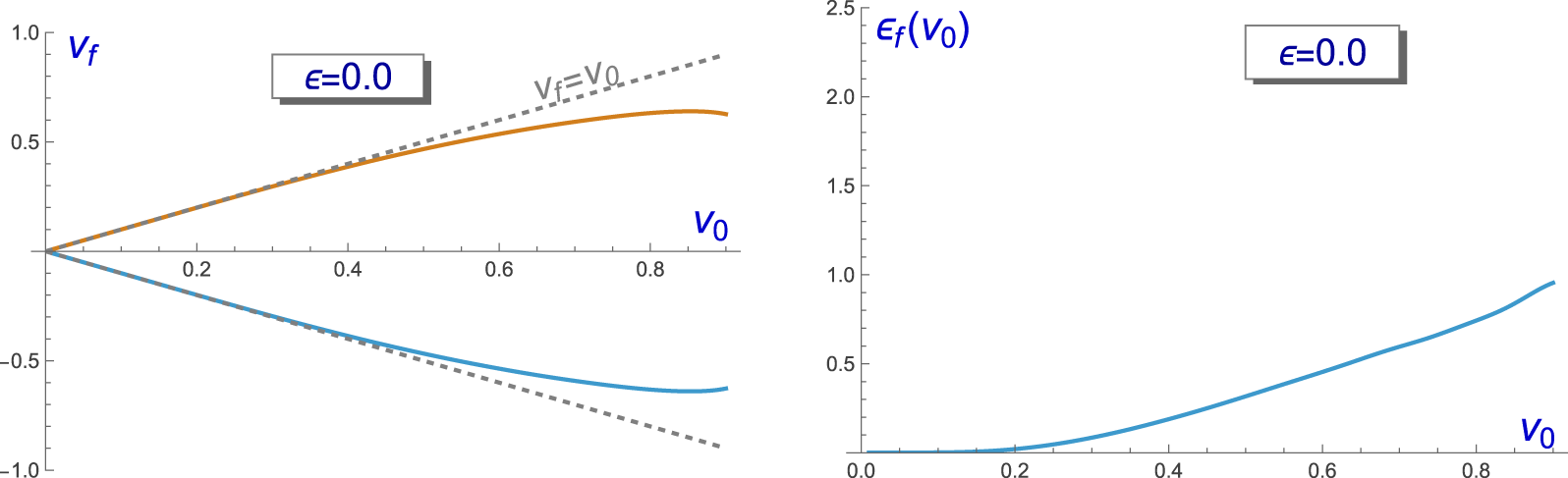
If the scattering process were perfectly elastic, the outgoing velocity would coincide with the initial one. In that case, the curve representing the final vortex velocity as a function of the initial collision velocity would be a straight line with unit slope. In Figure 8, the scattering diagrams for the collision of two unexcited vortices are displayed. Clearly, in Figure 8 (left), two different curves (plotted in blue and orange) are obtained, representing the final velocities of the two vortices that emerge after the collision in opposite directions along the same axis. The scattering remains nearly elastic for relatively small initial velocities, $v_0\leq 0.3$. However, for larger velocities, the outgoing velocity becomes progressively smaller than the initial one, indicating that part of the kinetic energy is transferred to other channels. In particular, a fraction of the energy is radiated away, while another portion is converted into internal vibrational energy of the vortices. This effect is confirmed in Figure 8 (right), where we plot the excitation amplitude $\epsilon_f$ of the outgoing vortices after the collision. As the initial velocity increases, the final excitation amplitude also grows, showing that the vortices emerge from the collision in a more strongly excited state. This behaviour clearly signals a departure from the adiabatic regime.

Figure 8.

Final velocity $v_f$ (left) and the excitation amplitude $\epsilon_f$ (right) of the outgoing vortices versus the initial collision velocity $v_0$ for the scattering of two unexcited 1-vortices. The dashed grey lines introduced in the first graphic correspond to perfectly elastic scattering.

As mentioned earlier, the main goal of this work is to show that the dynamics of vortices can be significantly modified when the defects are initially excited by the Derrick-type vibrational mode. To investigate this effect, we consider the same type of scattering processes analysed previously, but now involving vortices that carry an initial vibrational excitation. In this scenario, when the vortices collide, there are two relevant energy channels. On the one hand, the translational kinetic energy associated with the motion of the vortex centres is present, as in the unexcited case. On the other hand, the vortices also possess an additional reservoir of vibrational energy stored in their internal Derrick-type mode. As a consequence, during the collision process, the energy flow between these channels can be substantially different, leading to a modified scattering dynamics.

In order to gain analytical insight into the origin of these effects, we introduce a simple collective-coordinate description of this two 1-vortex scattering process as introduced in [Reference Izquierdo, Manton, Guilarte and Wereszczynski24]. Within this approach, the dynamical variables are restricted to the vortex centre $(x_1(t),x_2(t))$ and to the excitation amplitude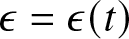 $\epsilon=\epsilon(t)$ associated with the internal mode. Using this ansatz, one can construct an effective Lagrangian for the reduced system, which takes the form

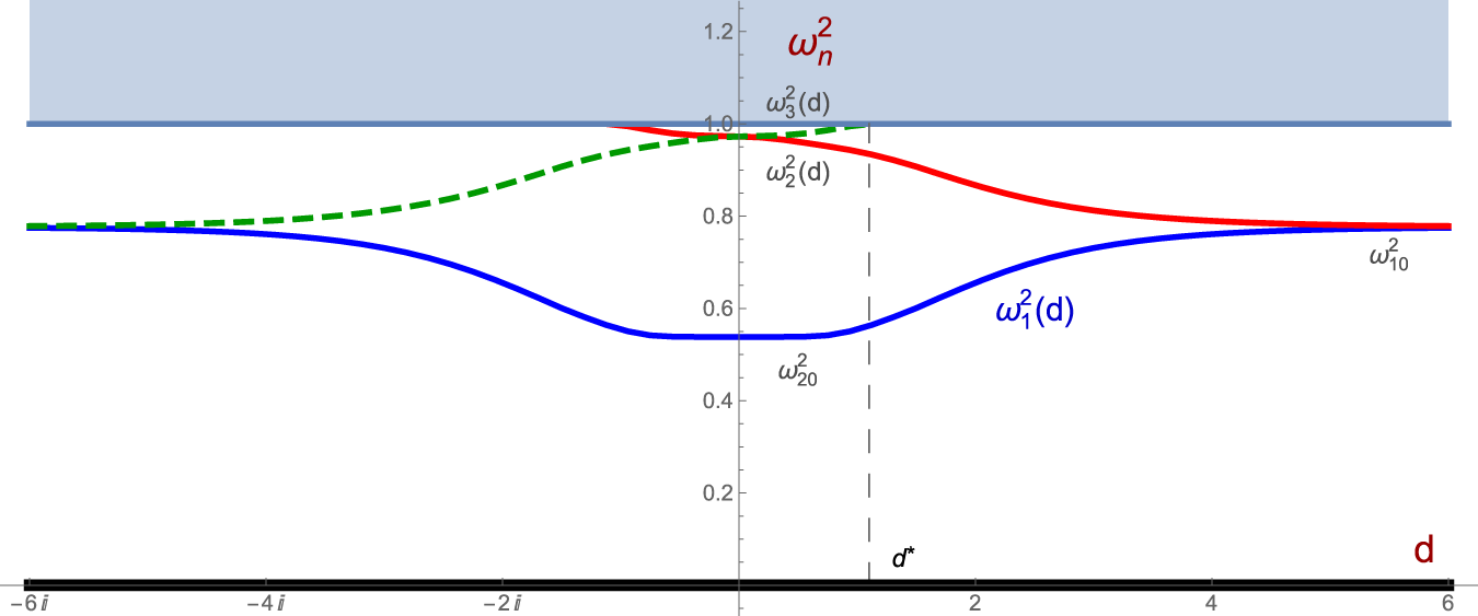
(4.1)\begin{equation} L = \frac{1}{2} \Omega(x_1,x_2,\epsilon) \left[ \left( \frac{dx_1}{dt} \right)^2 + \left( \frac{dx_2}{dt} \right)^2 \right] + \frac{1}{2} \left( \frac{d\epsilon}{dt} \right)^2 - \frac{1}{2} \omega_1^2(x,y) \, \epsilon^2 \end{equation}

Here $\Omega$ denotes a metric factor in the moduli space affecting the vortex position coordinates that can be obtained numerically from the zero modes of the theory. In the limit where the excitation vanishes, $\epsilon=0$, this factor reduces to the well-known Samols metric [Reference Samols35] that governs the dynamics of unexcited vortices. The inclusion of the additional dynamical degree of freedom associated with the vibrational amplitude $\epsilon$ modifies the structure of this metric. However, for the purposes of the present work, it is not necessary to explore the detailed properties of this generalized metric factor. Instead, our analysis focuses on the consequences of the last term appearing in the effective Lagrangian (4.1). This term is proportional to the square of the excitation amplitude $\epsilon(t)$. The proportionality factor is determined by the eigenvalues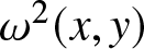 $\omega^2(x,y)$ of the spectral problem (3.4), which characterize the vibrational modes of the vortex configuration. Let us recall that in the self-dual regime of the Abelian-Higgs model, configurations with winding number $n=2$ correspond to two single vortices that can be placed at arbitrary positions on the plane. These configurations form a continuous family of static solutions parametrized by the positions of the vortex centres. As a consequence, the eigenvalues associated with the vibrational modes are not fixed constants but depend on the specific configuration of the two vortices. In particular, they depend on the separation $d$ between the vortex centres. This property implies the existence of a spectral flow controlled by the inter-vortex distance $d$. In other words, during the scattering of two vortices, the eigenvalues of the spectral problem evolve continuously as the vortices approach each other and subsequently move apart.

In Figure 9, we display the dependence of these eigenvalues as a function of the distance $d$. As shown, when the two vortices are excited in phase, the relevant eigenvalue follows the blue curve shown in the figure. In this situation, as the vortices approach each other from large separations, the frequency of their vibrational mode gradually decreases. The minimum value is reached when the vortices coincide at the same point in the plane, forming a rotationally invariant 2-vortex configuration. This behaviour has direct implications for the effective Lagrangian (4.1). Since the vibrational contribution to the energy involves the eigenvalue of the spectral problem, the variation of this eigenvalue with the vortex separation generates an effective interaction between the vortices. In particular, for in-phase excitations, the reduction of the vibrational frequency as the vortices approach each other translates into an effective attractive force mediated by the vibrational mode.

Figure 9.

Spectral flow of the vibrational eigenvalues for 2-vortex static configurations. The eigenvalues $\omega^2$ of the spectral problem (3.4) are plotted as a function of the inter-vortex distance $d$. The blue curve corresponds to in-phase excitations of the two 1-vortices.

Figure 9 Long description

The graph shows the spectral flow of vibrational eigenvalues omega subscript n superscript 2 as a function of inter-vortex distance d. The x-axis is labeled d, ranging from minus 6i to 6, with imaginary units marked at minus 6i, minus 4i, minus 2i. The y-axis is labeled omega subscript n superscript 2, ranging from 0.2 to 1.2. Three curves are plotted: omega subscript 1 superscript 2 open parenthesis d close parenthesis decreases from about 0.8 at d equals minus 6i to a minimum near 0.55 around d equals 0, then rises back to about 0.8 at d equals 6. Omega subscript 2 superscript 2 open parenthesis d close parenthesis starts near 1.0 around d equals 0 and decreases toward 0.8 as d increases. Omega subscript 3 superscript 2 open parenthesis d close parenthesis rises from about 0.8 at d equals minus 6i to near 1.0 around d equals 0. A vertical dashed line labeled d asterisk is slightly right of d equals 0, indicating a reference point. Additional labels include omega subscript 10 superscript 2 near 0.8 on the right and omega subscript 20 superscript 2 near 0.5 on the left, indicating specific eigenvalue levels.

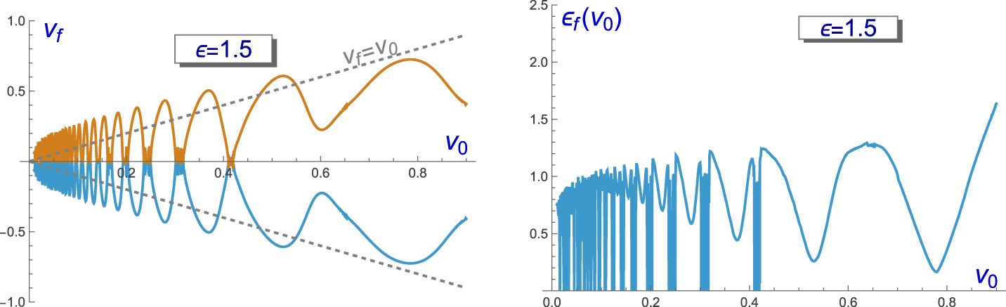
The presence of this mode-induced interaction can drastically modify the vortex dynamics. In particular, the outcome of scattering processes involving initially excited vortices may differ significantly from the behaviour observed when the vortices are unexcited, leading to qualitatively new dynamical regimes. This behaviour becomes particularly evident in Figure 10, where we display the dependence of the final vortex velocity and the final excitation amplitude on the initial collision velocity (along the $x_1$-axis) for head-on scattering processes involving vortices that are initially excited with a relatively large amplitude,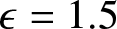 $\epsilon=1.5$. A comparison with the case of unexcited vortices reveals several striking differences, which we summarize below.

Figure 10.

Final velocity $v_f$ (left) and excitation amplitude $\epsilon_f$ (right) of the outgoing vortices as functions of the initial collision velocity $v_0$ (along the $x_1$-axis) for head-on scattering of two 1-vortices with initial excitation amplitude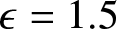 $\epsilon=1.5$. The dashed grey lines introduced in the first graphic correspond to perfectly elastic scattering.

Figure 10 Long description

The image A showing a line graph with the y-axis labeled v subscript f and the x-axis labeled v subscript 0. The x-axis runs from 0.0 to 0.9 with labeled ticks at 0.2, 0.4, 0.6 and 0.8. The y-axis runs from minus 1.0 to 1.0 with labeled ticks at minus 1.0, minus 0.5, 0.0, 0.5 and 1.0. A boxed label reads epsilon equals 1.5. Two oscillating curves are plotted, one above and one below the horizontal axis. A dashed diagonal reference line is labeled v subscript f equals v subscript 0, rising from near the origin toward the upper right. A second dashed diagonal line slopes downward from near the origin toward the lower right. The upper curve starts near 0 at v subscript 0 equals 0.0, shows many tight oscillations for v subscript 0 below about 0.2, then broader oscillations with peaks around 0.5 to 0.7 and troughs near 0.0 as v subscript 0 increases toward about 0.9. The lower curve starts near 0 at v subscript 0 equals 0.0, shows many tight oscillations for v subscript 0 below about 0.2, then broader oscillations with troughs around minus 0.5 to minus 0.8 and peaks near 0.0 as v subscript 0 increases toward about 0.9. The image B showing a line graph with the y-axis labeled epsilon subscript f open parenthesis v subscript 0 close parenthesis and the x-axis labeled v subscript 0. The x-axis runs from 0.0 to 0.9 with labeled ticks at 0.0, 0.2, 0.4, 0.6 and 0.8. The y-axis runs from 0.0 to 2.5 with labeled ticks at 0.5, 1.0, 1.5, 2.0 and 2.5. A boxed label reads epsilon equals 1.5. A single curve begins near the y-axis with many narrow spikes and drops between about 0.0 and about 0.25 on v subscript 0, then transitions into broader oscillations. The curve shows local maxima around 1.1 to 1.3 near v subscript 0 around 0.35 to 0.45, a dip near about 0.5, another rise near about 0.6 to 0.7 around 1.2 to 1.3, a dip near about 0.8 around 0.2 to 0.4 and then rises toward the right edge to about 1.6 near v subscript 0 around 0.9.

First, the most prominent feature is the emergence of a fractal structure in the diagram of final velocities. In particular, one observes a sequence of intervals in which the final velocity varies continuously from zero to a maximum value and back to zero. These intervals or velocity windows are reproduced at progressively smaller scales across different regions of the initial velocity axis, generating a self-similar pattern characteristic of fractal structures. Similar phenomena have previously been observed in the scattering of wobbling kinks in the $\phi^4$-model in $(1+1)$-dimensional spacetime [Reference Alonso-Izquierdo, Nieto and Queiroga-Nunes11, Reference Izquierdo, Queiroga-Nunes and Nieto25]. The origin of this behaviour is explained by the relative phase of the vortex oscillations at the moment of collision. Depending on whether the oscillation amplitude at that instant is close to its maximum, its minimum or an intermediate value, the amount and direction of energy transfer between the vibrational and translational degrees of freedom can vary significantly. Consequently, the detailed structure of the diagram may shift depending on the initial phase of the oscillation, which effectively translates the positions of the collision windows. Nevertheless, the overall fractal pattern remains unchanged.

Second, the scattering process is strongly inelastic, even at relatively small initial velocities. As a consequence of the resonant energy exchange mechanism, it is possible to observe final vortex velocities that exceed the initial collision velocity. In such cases, energy stored in the vibrational mode is transferred to the translational motion, leading to outgoing vortices that move faster than the incoming ones. The opposite process can also occur: for certain values of the initial velocity, energy is transferred from the translational degrees of freedom to the vibrational mode, resulting in outgoing vortices with lower velocities and significantly larger excitation amplitudes than those initially present. Examples of both behaviours are illustrated in Figure 11, where we display the trajectories of the vortex centres for two representative scattering events. The first case, shown in Figure 11 (left), represents the scattering of two in-phase excited 1-vortices with amplitude 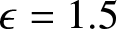$\epsilon=1.5$ approaching each other along the $x_1$-axis with an initial velocity $v_0=0.155$. As can be observed, after the collision, the vortices separate along the $x_2$-axis with a final velocity $v_f\approx 0.32$, larger than the initial one. In Figure 11 (middle), the initial collision velocity is increased to $v_0=0.408$, and in this case, the outgoing vortices move away with a smaller final velocity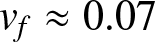 $v_f\approx 0.07$.

Figure 11.

Coordinates of the vortex centres as functions of time for the scattering of in-phase excited vortices with initial amplitude 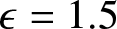$\epsilon=1.5$ and initial velocities $v_0=0.155$ (left), $v_0=0.408$ (middle) and $v_0=0.124$ (right). The blue and red curves correspond to the $x_1$- and $x_2$-components of the vortex positions.

Figure 11 Long description

The image A showing a line plot with a legend listing “Vortex Centers (x subscript 1 component)” and “Vortex Centers (x subscript 2 component)”. The horizontal axis is labeled t, with tick labels 20, 40, 60, 80, 100, 120. The vertical axis has tick labels 30, 20, 10, 0, minus 10, minus 20, minus 30. A boxed label reads v subscript 0 equals 0.155 and epsilon equals 1.5. Two solid curves meet near t about 60 at y about 0, then separate: one solid curve rises to about y 25 by t 120 and another solid curve falls to about y minus 25 by t 120. Two other solid curves approach y about 0 from about y 10 and y minus 10 as t increases toward about 60. Two dashed diagonal lines form an X shape centered near t about 60 and y about 0. The image B showing a line plot with a legend listing “Vortex Centers (x subscript 1 component)” and “Vortex Centers (x subscript 2 component)”. The horizontal axis is labeled t, with tick labels 20, 40, 60, 80, 100, 120. The vertical axis has tick labels 30, 20, 10, 0, minus 10, minus 20, minus 30. A boxed label reads v subscript 0 equals 0.408 and epsilon equals 1.5. Two solid curves meet near t about 20 at y about 0, then separate with smaller slopes than in image A: one solid curve rises to about y 8 by t 120 and another solid curve falls to about y minus 10 by t 120. Two other solid curves approach y about 0 from about y 10 and y minus 10 as t increases toward about 20. Two dashed diagonal lines form an X shape centered near t about 20 and y about 0. The image C showing a line plot with a legend listing “Vortex Centers (x subscript 1 component)” and “Vortex Centers (x subscript 2 component)”. The horizontal axis is labeled t, with tick labels 100, 200, 300, 400, 500, 600, 700. The vertical axis has tick labels 30, 20, 10, 0, minus 10, minus 20, minus 30. A boxed label reads v subscript 0 equals 0.124 and epsilon equals 1.5. Two solid curves oscillate around y equals 0 across the full time range, with repeated peaks and troughs staying close to the zero line. Near t about 100, one solid curve starts near y about 10 and decreases toward y about 0 while the other solid curve starts near y about minus 10 and increases toward y about 0.

Finally, in the regions between the velocity windows described above, the resonant energy transfer mechanism becomes even more pronounced. In these intervals, the vortices may undergo multiple collisions before eventually separating. During these repeated interactions, energy is exchanged back and forth between the vibrational and translational degrees of freedom until the system reaches a configuration where the vortices can escape. An example of this behaviour is shown in Figure 11 (right), where the two 1-vortices undergo multiple $90^\circ$ collisions.