


1. Introduction
Incentives have to matter. This imperative is a core tenet of economics. Insufficient or inadequate incentives will lead to deviations in the behavior predicted by economic and behavioral models. Economic experiments often involve multiple decisions of the same task, or they incorporate multiple tasks within the same study. Correspondingly, researchers must weigh the potential tradeoffs of different payment mechanisms, the size of incentives, potential payoff externalities, and budget constraints. Paying for every decision increases costs and may induce portfolio and wealth effects. While these effects can be mitigated by only paying for one random choice, paying for one random choice may dilute incentives as the number of choices increases (Beattie & Loomes, Reference Beattie and Loomes1997; Charness et al., Reference Charness, Gneezy and Halladay2016). To complicate matters further, random incentive schemes may fail to be incentive-compatible, exhibit menu dependence, and induce risk preferences even in purely deterministic settings. This shortcoming of random incentives has led some researchers to argue for collecting preferences only over a single choice (e.g., Cox et al., Reference Cox, Sadiraj and Schmidt2015; Harrison & Swarthout, Reference Harrison and Swarthout2014), despite the restrictive nature of this approach. Overall, the first-best incentive scheme is rarely transparent, making it difficult to develop general guidelines.
The lack of empirical interest, even from experimental economists (Azrieli et al., Reference Azrieli, Chambers and Healy2018), suggests that incentive compatibility concerns may be overstated. More troubling, perhaps, is the fact that the incentive compatibility of different mechanisms cannot be established without particularly strong assumptions on preferences. For example, most theoretical work focuses on menu-independent binary preferences. Paradoxically, these preferences may not exist if agents have non-consequentialist preferences, e.g., non-expected utility preferences (Machina, Reference Machina1989). Moreover, incentive compatibility has little explanatory power for plausible mistakes or heuristics. How, then, can one elicit true preferences and discriminate among existing preference incentive mechanisms?
Our study employs the simplest application of induced values (Smith, Reference Smith1976), providing a straightforward empirical testing approach: the monetary value of money is known. Consequently, for all of our extensive experimental treatments, the objective preferences over monetary amounts are clearly defined in terms of their monetary equivalents. Thus, we can focus primarily on the proper empirical incentive scheme. That is, on the effectiveness of different incentive schemes to recover correct individual preferences from the (induced) preferences. In a nutshell, the known monetary value of  $\$2$ is $\$2$, as used by Cason and Plott (Reference Cason and Plott2014).
In a sample of these valuation tasks, we consider, broadly, the following three dimensions of incentive mechanisms: 1) the size of the prize, 2) the chance with which payment is determined, i.e., the “incentive scheme,” and 3) the chance each choice counts toward total earnings, i.e., the “payment mechanism.” In the valuation tasks, we also vary the range of values people can assign to a certain monetary amount and whether the uncertainty determining earnings is strategic.
In a collective sample of over 3,000 subjects, we find that subjects are sensitive to changes in prizes and that the problem’s framing matters, while the incentive scheme and the payment mechanism empirically do not. Participants exhibit greater sensitivity to monetary rewards, as reflected in better-calibrated valuations for higher rewards, while broader value ranges (greater opportunity for deviations) lead to higher deviations from the objective monetary value of a dollar. Strikingly, the lack of variation according to the incentive scheme extends to cases where the rewards are hypothetical, adding to the literature that finds minimal or no differences between real and hypothetical stakes (e.g., Brañas Garza et al., Reference Brañas Garza, Jorrat and Espín2023; Enke et al., Reference Enke, Gneezy, Hall, Martin, Nelidov, Offerman and van de Ven2023; Gneezy et al., Reference Gneezy, Imas and List2015; Hackethal et al., Reference Hackethal, Kirchler, Laudenbach, Razen and Weber2023; Li et al., Reference Li, Müller, Wakker and Wang2017; Irwin et al., Reference Irwin, McClelland and Schulze1992).Footnote 1 One reason why the incentive scheme may not yield any meaningful effects is that the evaluated tasks (preference elicitations) are not cognitively demanding, or that higher cognitive effort may not lead to a meaningful difference between hypothetical and real behavior. We also find that strategic uncertainty produces better-calibrated valuations; however, different incentive schemes again play no meaningful role in overall bidding behavior. Although misunderstanding may be a factor explaining misbehavior (Serizawa et al., Reference Serizawa, Shimada and Tse2024), we doubt that it is driving our results, given the strict measures taken to ensure that subjects were attentive to the instructions and understood the procedures.
The rest of the paper proceeds as follows. The next section reviews the relevant literature to set the context and motivate our study. We then present the two experiments sequentially by describing the methods and summarizing the results from each experiment. We conclude in the final section.
2. Related literature
This section briefly reviews some of the existing literature on the effect of payment mechanisms on experimental auctions and Between-Subject Random Incentive Schemes (BRIS). We highlight key studies and findings in the field, revealing the complexities and debates surrounding effective incentive design, the role of cash balances, and the effectiveness of different incentivization strategies. This overview offers insights into how experimental setups and incentive mechanisms can significantly affect economic behavior and decision-making processes.
Early studies in the auction literature investigating the winner’s curse sparked debates due to the use of mechanisms that involved paying for all decisions across multiple periods (Kagel & Levin, Reference Kagel and Levin1986). Hansen and Lott (Reference Hansen and Lott1991) argued for the rationality of subject bids above the auctioned item’s conditional expected value at the theoretical bidding equilibrium observed in Kagel and Levin (Reference Kagel and Levin1986) as a response to limited liability and low cash balances (i.e., accumulated earnings from paying for multiple rounds).Footnote 2
In response, Kagel and Levin (Reference Kagel and Levin1991) conducted a follow-up experiment that ensured subjects had sufficient cash balances so that deviations from the predicted (risk-neutral) Nash equilibrium could not be explained by the limited liability arguments and still obtained significant overbidding. Ham et al. (Reference Ham, Kagel and Lehrer2005) argued that cash balances may also affect bidding behavior in private value auctions, and to address this concern, they introduced exogenous variation in cash balances by randomly assigning additional payments while subjects bid in a first price auction. They found that cash balances also play a statistically significant role in bidding behavior in private value auctions.
While cash balance incentives can be avoided by paying for only one randomly selected trial, Ham et al. (Reference Ham, Kagel and Lehrer2005) further noted their impact on subjects’ incentives, potentially diluting payoffs in two ways. First, expected payoffs can be a function of the compounded probability of a trial being selected multiplied by the payoffs for that trial, which may dilute incentives with an increased number of trials and/or smaller payoffs per trial. Second, since there is only one bidder with earnings in many auction formats, as in a first or a second price auction, effective recruitment of subjects can only be achieved with large fixed show-up fees, which may render the incentives associated with the auctions trivial.Footnote 3
Also relevant to our study is a strand of the literature that has focused on Between-Subject Random Incentive Schemes (BRIS) or lottery incentives, where only a subset of subjects are randomly selected to realize their decisions and receive a payment. BRIS has been investigated in several domains including fairness (Bolle, Reference Bolle1990), preferences for risk and ambiguity (Anderson et al., Reference Anderson, Freeborn and McAlvanah2023; Aydogan et al., Reference Aydogan, Berger and Théroude2024; Baltussen et al., Reference Baltussen, Post, van-den Assem and Wakker2012; Berlin et al., Reference Berlin, Kemel, Lenglin and Nebout2026; March et al., Reference March, Ziegelmeyer, Greiner and Cyranek2016), time preferences (Berlin et al., Reference Berlin, Kemel, Lenglin and Nebout2026) and donations in dictator games (Clot et al., Reference Clot, Grolleau and Ibanez2018). More recently, Ahles et al. (Reference Ahles, Palma and Drichoutis2024) found that a 10% and 1% payment probabilities are effective in eliciting valuations that are statistically indistinguishable from a fully incentivized scheme and that all incentivized conditions can mitigate hypothetical bias, resulting in lower elicited valuations than a purely hypothetical condition. Ahles et al. (Reference Ahles, Palma and Drichoutis2024) is likely the first systematic work on BRIS in valuation research, serving as the foundation for subsequent studies that have built upon and applied their methods in valuation settings (e.g., Bó et al., Reference Bó, Chen and Hakimov2024; Hosni et al., Reference Hosni, Segovia and Zhao2024; Mustapa et al., Reference Mustapa, Kallas, López-Mas, Alamprese, Contiero and Aguiló-Aguayo2025; Veettil et al., Reference Veettil, Yashodha and Vecci2025).
3. Experiment 1: preference elicitation with the BDM mechanism
The following section first outlines the experimental design and implementation details, including subject recruitment, instructions, task structure, and treatment arms. We then present the main empirical results.
3.1. Methods and experimental design
This study and the subsequent study described in the next section were preregistered with the AEA’s RCT registry (AEARCTR-0009687). Subjects were panelists from Forthright Access, an online research company that handles its own recruitment through various direct advertising channels. Participants were offered a $2.5 reward for a 20-minute study. Subjects were informed they could also gain additional rewards after entering the study. We employed several quality controls to ensure subjects’ attention and comprehension based on a pilot study with 78 subjects (Haaland et al., Reference Haaland, Roth and Wohlfart2023).Footnote 4
Experiment 1 involved eliciting preferences over an induced value (IV) using the BDM mechanism (Becker et al., Reference Becker, DeGroot and Marschak1964). As in Cason and Plott (Reference Cason and Plott2014), subjects were endowed with a card worth a known IV and were asked to state their offer price to sell the card back to the experimenter.Footnote 5 Subjects were informed that their offer price would be compared to a fixed offer that would be randomly drawn from the interval of  $[0,X]$ where $X$ was varied from task to task.Footnote 6 We varied the IV at a low and a high level of $1 and $3 and varied the maximum bid range, $X$, at $4, $5, and $6. Consequently, each subject participated in six tasks; all possible combinations of the IV and the upper level of the support of the distribution, $X$. The order of the six preference-elicitation tasks was randomized across subjects.
The instructions included several examples detailing the BDM mechanism, followed by a series of true/false and open-ended comprehension questions. Although we provided detailed instructions and examples to ensure that participants understood the mechanisms in the study, we did not instruct participants on what to bid or explicitly guide their behavior.Footnote 7 After screening out inattentive subjects, the sample included 2,575 subjects.Footnote 8 In addition to the participation fee, subjects analyzed in this paper earned an average of $2.67 (min=$0, max=$29.4, SD=$5.82).
Our experimental design also varied on two between-subjects dimensions: incentive schemes and payment mechanisms.Footnote 9 To test for potential diluted incentives, we had three different likelihoods of decisions being paid in the incentive scheme: subjects either had a 100% chance of receiving monetary rewards associated with their decisions, a 50% chance, or a 1% chance. After collecting data for these treatments, we found a null effect of differences between treatments, so we decided to run two additional boundary conditions: a 0.2% chance treatment of getting monetary rewards and a purely hypothetical treatment. Thus, the incentive scheme had five distinct probabilities of payment for subjects. Every subject was given information about the probability of their decisions being paid in two different screens: one at the beginning of the study and one right before eliciting their preferences with a BDM mechanism. For the hypothetical treatment, subjects were informed multiple times at different points of the study that although monetary rewards would be shown in various screens, they would only receive a fixed compensation and that none of the stated monetary amounts would count toward their earnings. The text in the instructions was modified appropriately for the corresponding treatments, varying the probability of payments. The instruction scripts appear in the Online Appendix.
The second dimension, the payment mechanism, varied the number of paid decisions, the correlation between those payments, and whether we adjusted the magnitudes according to the number of paid decisions. Our base payment is the Pay-One-Randomly (POR) mechanism, where only one of the six tasks is randomly selected for payment. We compare the POR mechanism with four additional payment mechanism previously used by Cox et al. (Reference Cox, Sadiraj and Schmidt2015) (in an application of decisions under risk): (a) the Pay-All-Correlated (PAC) mechanism, (b) the PAC mechanism adjusted for the number of tasks (PACn), (c) the Pay-All-Independently (PAI) mechanism and (d) the PAI mechanism adjusted for the number of tasks (PAIn).Footnote 10 For the PAC mechanism, subjects were paid for all six preference elicitation tasks, with the fixed offer determined with a single draw for all tasks as follows: a random percentage would be drawn between 0% and 100%, and the drawn percentage would be multiplied by the upper support of the distribution of allowed offers which would determine the fixed offer per task, albeit with a single draw. An arithmetic example illustrated this mechanism for subjects. The PACn mechanism was explained in a similar fashion, albeit subjects were aware that they would receive one-sixth of the total payoffs (therefore, the payoffs were divided by the number of tasks).
In the PAI mechanism, subjects received an independent draw per task as follows: subjects were informed that the computer would choose a random percentage for each task that would be multiplied by the upper support of the distribution of allowed offers, which would determine a different fixed offer per task. An arithmetic example illustrated this mechanism for subjects. The PAIn mechanism was explained in a similar way to PAI with the difference that subjects were told they would receive one-sixth of the total payoffs.
Table 1 summarizes the experimental design and the number of subjects assigned to each treatment arm. Our target of 100 subjects/treatment is large enough to detect minimum differences in absolute bid deviations (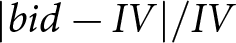 $|bid-IV|/IV$) of 0.05 or larger with 80% power. Sample size calculations, instructions, examples, and final payoff screens are provided in the Online Appendix, which can also be consulted at the Open Science Framework.
Experimental design and number of subjects per treatment

Notes: PAC, PAI, and POR stand for pay-all-correlated, pay-all-independently, and pay-one-randomly, respectively. n indicates the sum of payoffs is divided by the number of tasks.
3.2. Experiment 1 results
Figure 1 shows CDFs of bid deviations from the IV (Panel a) and relative absolute deviations from the IV (Panel b).Footnote 11 It is clear that greater misbidding occurs for the lower IV as the respective CDF is shifted more to the right.Footnote 12 Figure 1(a) also shows that overbidding is more prevalent than underbidding. Only 15.50% of all bids are exactly equal to the IV and 24.71% (30.89%) of all bids are within 5% (10%) of the IV. Cason and Plott (Reference Cason and Plott2014) report that without training 16.7% of subjects have bids within 5 cents (2.5%) of their induced value of  $\$2$, which is similar to our findings. Moreover, Brown et al. (Reference Brown, Liu and Tsoi2025) find similar patterns of misbidding that are fairly constant across various elicitation formats that are strategically equivalent but cognitively simpler than the BDM mechanism.
CDFs of bid deviations from IV (BDM). (a) Bid deviations from IV. (b) Relative absolute bid deviations from IV

Table 2 shows descriptive statistics (mean, standard deviation, median) for the relative absolute deviations by incentive scheme and payment mechanism. The values of the deviations in this table are remarkably stable across treatments at around 0.5, supporting a statistically insignificant effect of both incentives schemes and payment mechanisms.Footnote 13
Descriptive statistics of 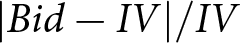 $|Bid-IV|/IV$ by payment mechanism and incentive scheme

Notes: This table shows means, standard deviations in parenthesis and medians in brackets, pooled across the six decisions. PAC, PAI, and POR stand for pay-all-correlated, pay-all-independently, and pay-one-randomly, respectively; n indicates the sum of payoffs is divided by the number of tasks.
Table 3 shows estimates from regression models with clustered standard errors at the individual level, using either bid deviations ( $Bid - IV$) or relative absolute deviations ( $|Bid-IV|/IV$) as the dependent variable and the treatment indicators as independent variables.Footnote 14
Regressions of bid deviations on treatment variables

Notes: Clustered standard errors in parentheses.
* p $ \lt $0.1, **p $ \lt $0.05 and ***p $ \lt $0.01. Base categories for the treatment variables are: IV = 1 & Support = 4, 100% & POR. PAC, PAI, and POR stand for pay-all-correlated, pay-all-independently, and pay-one-randomly, respectively. n indicates the sum of payoffs is divided by the number of tasks.
As shown in Table 3, relative to the 100% incentives scheme in the POR baseline payment mechanism, none of the incentives schemes nor the payment mechanisms significantly affect misbidding behavior. None of the coefficients is statistically different from the baseline. On the other hand, both the IV and the support level of the distribution affect deviations from the induced value. More specifically, the upper panel of Table 3 shows that a larger induced value reduces deviations from the IV and that this reduction is moderated by the level of the support of the distribution. For the lower IV of $1, a larger support increases relative absolute misbidding by 0.17 to 0.39. The larger IV of $3 reduces misbidding behavior but with a larger support this reduction shrinks. For example, model (1) shows that misbidding declines by 0.76 for a $4 support, but it is only reduced by 0.31 for the larger level of support of $6.Footnote 15
Additional analysis in Section B in the Online Appendix estimates ordered logit models by transforming the dependent variable to categories (under/over bids and bids equal to the IV). Results are similar to what was discussed above.
4. Experiment 2: preference elicitation with the Second Price Auction
To test whether the preference elicitation mechanism has an effect on elicited preferences, in Experiment 2, we replaced the BDM mechanism with the Second Price Auction (SPA). Both BDM and SPA are theoretically incentive compatible, but the SPA features strategic uncertainty, as opposed to personal or objective uncertainty, as the uncertainty arises from other bidders’ strategy rather than a randomly drawn price. Although this should not influence (equilibrium) behavior, replacing the BDM with an SPA allows us to empirically test whether the source of the uncertainty matters. Varying the source of uncertainty helps us understand whether the randomization devices being employed may be driving our results. We reduced the treatment arms of the experimental design of Experiment 1 to fit budget constraints and selected to test a subset of treatments that are most widely used and provide boundary conditions, since they may be more likely to affect bidding behavior. With respect to the incentive schemes, we administered a purely hypothetical treatment and a treatment that pays with 100% certainty. With respect to the payment mechanisms, we selected the POR and the Pay-All divided by the number of rounds (PAn) in order to keep incentives comparable.Footnote 16 In summary, we implement a 2 $\times$2 between-subjects design in Experiment 2.
4.1. Methods and experimental design
Subjects were panelists from Forthright Access, none of whom had participated in Experiment 1. We offered a $2 reward for a 15-minute study. Subjects that were not assigned to a hypothetical treatment were informed they could also earn additional rewards after entering the study.
We implemented the same quality controls as in Experiment 1. One particular feature of this experiment is that recruitment was done on a limited time window within a day to ensure a large pool of participants entered simultaneously and achieve good matching of participants to the auction groups. Four subjects would form an auction group, but if more than 3.5 minutes elapsed without fulfilling a group, then we used bots to complement a group.Footnote 17 The main results present responses from subjects who were matched in groups of humans only. The results that include subjects matched with bots are presented in the Online Appendix and are similar to the humans-only sample. Subjects were informed about the number of bots they were matched with, if any. Furthermore, when we control for the number of bots in the regressions shown in the Online Appendix, we find that the inclusion of bidding bots does not significantly affect the results. All subjects in a group were assigned to the same treatment for the entire experiment.Footnote 18
The final sample with complete responses includes 637 subjects, albeit 209 of them were matched with one or more bots. On top of their participation fee, subjects received an average of $1.06 (min=$0, max=$3, SD=$1.12). Table 4 shows the number of subjects per treatment. In the main regressions, we only use observations from subjects that were not matched to bots. Still, we controlled for the number of bots in additional specifications shown in the Online Appendix, and all of our results hold.
Experimental design, number of subjects, and number of bots per treatment

Notes: PA and POR stand for pay-all and pay-one-randomly, respectively; n indicates the sum of payoffs is divided by the number of tasks.
Similar to Experiment 1, subjects were endowed with a card worth a known IV and were asked to state their offer price to sell the card back to the experimenter with the understanding that they were assigned to a group of four subjects, their offer is compared to all other offers, and the lowest offer is accepted, but that the second lowest offer is the binding price. Subjects experienced four different IVs that were selected to be in the same range as in Experiment 1: $1, $1.7, $2.4, and $3. Subjects experienced all the IVs in a random order, and at any given round, only one subject was assigned to each IV so that all four IVs were assigned at any round.
Before participating in the SPA, all subjects went through similar instructions, comprehension questions, and quality checks as in Experiment 1. All experimental instructions, test questions, and attention check questions are provided in the Online Appendix, which is also available at the Open Science Framework.
4.2. Experiment 2 results
Figure 2 shows CDFs of bid deviations from IV (Panel a) and relative absolute deviations from IV (Panel b) for two of the IVs.Footnote 19 We purposefully keep the scale of the x-axis similar to Figure 1 to facilitate the visualization of the differences to the BDM mechanism in Experiment 1. The results show evidence that the SPA leads to less misbidding than the BDM and that a larger IV reduces misbidding. In the SPA, 19.98% of all bids are exactly equal to the IV, and 27.45% (42.93%) of all bids are within 5% (10%) of the IV. This is a substantial improvement compared to the BDM mechanism in Experiment 1.
CDFs of bid deviations from IV (SPA). (a) Bid deviations from IV. (b) Relative absolute bid deviations from IV

Table 5 shows estimates from regression models with clustered standard errors at the individual level, where we regressed either bid deviations ( $Bid - IV$) or relative absolute deviations ( $|Bid-IV|/IV$) on the treatments dummies. The sample is restricted to subjects that were not matched with a bot for the SPA.Footnote 20
Regressions of bid deviations on treatment variables for the SPA

Notes: Clustered standard errors in parentheses.
* p $ \lt $0.1, **p $ \lt $0.05 and ***p $ \lt $0.01. Base categories for the treatment variables are: IV = 1, Hypothetical, and POR. PA and POR stand for pay-all and pay-one-randomly, respectively; n indicates the sum of payoffs is divided by the number of tasks.
Results are similar to the general pattern we observe with the BDM mechanism. Higher IVs reduce the level of misbidding; however, misbidding is unresponsive to the payment mechanism and the incentive scheme, i.e., whether the treatment is hypothetical or real.
4.3. The BDM mechanism vs. the SPA
The average difference of 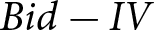 $Bid-IV$ is 0.29 in the BDM and -0.16 in the SPA, indicating that subjects on average overbid in the BDM mechanism and underbid in the SPA. In terms of absolute relative deviations ( $|Bid-IV|/IV$), subjects deviate on average 51.9% in the BDM mechanism and around 17.4% in the SPA indicating a substantially lower level of misbidding in the SPA. The magnitude of the improvement with the SPA is large.
To quantify and statistically test these differences, we also regressed bid deviations on the SPA dummy and demographic controls (standard errors are clustered at the individual level), and confirm that the SPA elicits smaller deviations from IVs (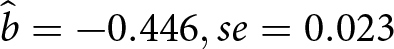 $\hat{b}=-0.446, se=0.023$). Similarly, for absolute bid deviations, the SPA elicits 33.9% smaller bids than the BDM ( $se=0.012$).
Section C in the Online Appendix shows additional analysis where we explore whether subjects’ behavior is consistent with game form misconception. While we find no differences in the payment mechanisms and incentive schemes, design features such as the IV and the support of the distribution have an impact on the bidding behavior. The results also clearly indicate that the SPA induces behavior that is closer to the IV and reduces the likelihood of misbidding compared to the BDM mechanism.
5. Discussion and conclusions
While most previous work on incentive-compatible payment schemes is theoretical, this paper explored the effects of incentive schemes and payment mechanisms in economic experiments using an empirical approach that focuses on value elicitation across two experimental studies with a large sample. Given the abundant literature showcasing empirical deviations from theoretical expectations, we argue that an empirical approach is needed in the incentives and payment mechanisms argument to voice the outcomes produced by participants in experiments. We found that while the nature of the incentive – hypothetical or real – had minimal impact on participants’ bidding behavior, the design elements, such as the magnitude of induced values and the range of offers, significantly influenced outcomes. Specifically, larger induced values and smaller offer ranges led to more accurate bidding, aligning closer to theoretical expectations. Therefore, our results suggest that design elements in the experiment environment may influence decision-making more than the incentive scheme.
Comparing the BDM mechanism (personal uncertainty) with the SPA (strategic uncertainty), the latter showed an improvement in aligning bids with the induced values, indicating that SPA produces less missbidding than the former. When comparing different payment mechanisms, decision-making noise and misconceptions about payoff functions were minimal across both auction mechanisms. A potential source that may be driving differences between the BDM and the SPA (and one that we cannot answer with the current set of experiments) is failures of contingent reasoning, that is, the cognitive difficulties faced by subjects when considering all the possible outcomes (Martínez-Marquina et al., Reference Martínez-Marquina, Niederle and Vespa2019). Assuming behavior might be influenced by the distribution of others’ bids (Georganas et al., Reference Georganas, Levin and McGee2017, find that subjects respond systematically to out-of-equilibrium incentives in SPAs), a subject may go through more strenuous mental gymnastics in the BDM mechanism to consider all possible contingencies; hence, the lower rate of mistakes in the SPA. Others have argued that the shape of the payoff function renders individual deviations from optimal behavior more costly in percentage terms in the SPA than in the BDM mechanism, and the loss from deviations is increasing in the number of bidders (Noussair et al., Reference Noussair, Robin and Ruffieux2004).
Our findings suggest that the effectiveness of incentive mechanisms in eliciting underlying preferences in economic experiments is complex. While certain design elements like the magnitude of rewards and range of offers play a critical role, the choice of elicitation mechanism (BDM vs. SPA) also significantly impacts the accuracy of outcomes. These uneven behavioral responses highlight the need for careful consideration of behavioral factors in experimental design to ensure the reliability and validity of results in economic research. We note that we included strict attention checks, which may be distinct from other studies.
We conclude by asserting the growing need to understand the complex interplay between cognitive effort and improved choices. The mounting number of perplexing null results on hypothetical bias can only be explained by securing a tighter grasp on this relationship. We call these results perplexing because even theoretically improper incentives yield identical responses. At the same time, more opportunities for mistakes and more complex decision problems can exacerbate differences both between and within methods. It is imperative that we learn more about the empirical nature of payment mechanisms to counterbalance the predominantly theoretical nature of the existing literature.
Supplementary material
The supplementary material for this article can be found at https://doi.org/10.1017/eec.2026.10042.
Acknowledgements
Part of this work was completed while Andreas Drichoutis was a Fulbright Visiting Scholar at Texas A&M University. We would like to thank Tim Cason and Uri Gneezy for helpful comments. We received financial support for this project from the Institute for Advancing Health through Agriculture at Texas A&M University. The replication material for the study has been deposited with the Open Science Framework at https://doi.org/10.17605/OSF.IO/2QPNW.


 Open access