


1. Introduction
Human life expectancy continues to rise, and a large part of the world has entered an era of population ageing. The United Nations describes a country as an “ageing society” if more than 7% of its population are aged 65 years and above, an “aged society” if this proportion exceeds 14%, or a “super-aged society” if it surpasses 21% (OECD/World Health Organization, 2022). As of 30 June 2023, 17.1% of Australians were aged 65 years and over (Australian Bureau of Statistics, 2024), indicating that Australia is already an aged society and rapidly approaching the super-aged status.
While increased longevity is a cause for celebration, living longer does not always equate to enjoying better health. The balance between years lived in good health and those with disabilities or chronic illnesses carries significant financial implications for healthcare systems and retirement planning. Decisions made by governments or organisations often take years to show tangible outcomes and have long-term ramifications. Accurate predictions are essential for policymakers and healthcare experts to allocate resources wisely and focus on health initiatives with the greatest potential benefits. Similarly, appropriate forecasting can support retirement planning by helping governments and institutions design sustainable pension systems, savings schemes, or retirement products to accommodate an ageing population. Moreover, assessing alternative scenarios can play a crucial role in uncovering uncertainties and addressing possible risks. One such application is in the planning and management of retirement villages, where reliable projections help ensure the provider’s financial viability.
While a substantial number of studies have been conducted on modelling mortality rates (Lee and Carter, Reference Lee and Carter1992; Cairns et al., Reference Cairns, Blake, Dowd, Coughlan, Epstein, Ong and Balevich2009; Haberman and Renshaw, Reference Haberman and Renshaw2011), relatively little attention has been paid to modelling and forecasting disability prevalence. Unlike mortality data which are generally widely accessible, health-related data are often limited and has to be compiled from various sources, making it more challenging to have detailed modelling of disability prevalence rates. Cao et al. (Reference Cao, Hou, Zhang, Xu, Jia, Sun, Sun, Gao, Yang, Cui, Wang and Wang2020) utilise multiple linear regression and autoregressive integrated moving average (ARIMA) models to forecast the so-called healthy life expectancy, which represents the number of healthy years an individual is expected to live. Lynch et al. (Reference Lynch, Bucknall, Jagger and Wilkie2022) employ a three-state model alongside the Lee and Carter (Reference Lee and Carter1992) method to project healthy working life expectancy. Li (Reference Li2024a, Reference Lib) establish Bayesian models to jointly model life expectancy and healthy life expectancy. Despite the useful insights provided by these recent efforts, their modelling primarily relied on healthy life expectancy data, which are essentially a summary metric of both disability prevalence and mortality rates. This indirect approach may obscure critical information about the morbidity trends embedded within the underlying rates.
In this paper, we take a different approach by developing Bayesian common factor models for modelling Australian age- and sex-specific disability prevalence rates directly. The proposed models incorporate one or more common factors shared by both sexes, as well as sex-specific factors. There are a number of methodological and practical contributions in this study. First, the proposed approach deals with the disability prevalence rates directly rather than an aggregate measure and so reveals the underlying disability trends clearly. Second, it uses cohort-specific probabilities, which are more realistic for computing the retirement management cash flows. Third, by employing the common factor model structure, it ensures internal consistency in handling mortality and prevalence rates. Moreover, Li (Reference Li2014) has noted several benefits of using Bayesian modelling which are applicable to our work here. First, the missing values in our disability prevalence data can be imputed automatically in the simulation process. This feature offers a practical way to handle the limitations of the prevalence data collected. Second, the Bayesian framework allows for coherent integration of the disability model structure and the time series process. The estimation of the two structures’ parameters occurs in the same process, avoiding the estimation bias that can arise with the traditional multi-step estimation setup. Furthermore, Bayesian modelling accounts for both process uncertainty and parameter uncertainty, while also enabling computation of prediction intervals. The simulated outputs provide a reasonable description of different risks and are useful for valuation applications. We adopt the software WinBUGS (Spiegelhalter et al., Reference Spiegelhalter, Thomas, Best and Lunn2003) to generate Markov chain Monte Carlo (MCMC) simulations.Footnote 1
In the literature, a common approach is to use multi-state models to capture transitions between different health states. Traditionally, these models assume time-homogeneous transition rates. For example, Riffe et al. (Reference Riffe, Ugartemendia, Tursun-zade and Muszyńska-Spielauer2024) use multi-state transition probabilities from Italian data to estimate the joint distribution of years spent in good and poor health. More recently, some studies allow transition rates to vary over time. Levantesi et al. (Reference Levantesi, Menzietti and Nyegaard2024) model morbidity intensity using a Cox–Ingersoll–Ross framework with Italian data, although the model assumes mean reversion and does not capture long-term trends. Zhou and Dhaene (Reference Zhou and Dhaene2024) adopted the modelling of transition intensities via the Cox regression approach with trend and frailty components calibrated by Sherris and Wei (Reference Sherris and Wei2021) on US Health and Retirement Study data. These latest time-varying multi-state modelling approaches generally require highly detailed longitudinal data, which may not always be available for insurance and financial applications.
Unlike multi-state models that estimate transition intensities between health states, our Bayesian common factor approach directly models age- and sex-specific disability prevalence rates. Disability prevalence represents only a snapshot of the proportion of the population living with disability at a given time, but the proposed approach allows us to use cross-sectional data rather than detailed longitudinal follow-up. It is more practical and convenient, particularly in contexts where individual-level transition data are sparse or incomplete. It also captures overall trends and shared patterns across sexes while also accounting for sex-specific deviations. A limitation, however, is that it does not explicitly model the timing or pathways of transitions between health states and cannot directly provide short-term stochastic dynamics at the individual level. Nevertheless, by focusing on disability prevalence, it offers a robust framework for projecting population-level disability outcomes and their corresponding financial consequences.
With the challenges of an ageing population becoming more pronounced, both governments and industry professionals are striving to formulate practical strategies to tackle the financial pressures associated with rising life expectancy. Older individuals face not only the risk of outliving their financial resources, often referred to as individual longevity risk, but also other personal challenges such as loneliness and social isolation. To address some of these needs, retirement villages have become an increasingly attractive option for many Australian seniors (Crisp et al., Reference Crisp, Windsor, Butterworth and Anstey2013), with the market growing by about 2–3% annually. They are specially designed residential communities where relatively healthy retirees live as neighbours and share a communal lifestyle (Hu et al., Reference Hu, Xia, Skitmore, Buys and Zuo2017). Typical motivations for choosing this type of arrangement include the increasing preference of a small family, the social support provided by fellow residents, and financial constraints. These communities cater to individuals who can manage daily living on their own. When a resident’s health deteriorates beyond a specified threshold, the contract ends, and the individual transitions to an aged care facility. In today’s market, retirement villages offer various accommodation styles that include diverse amenities and services, most of which are operated by for-profit financial organisations. The cost of these services depends on the resident’s total length of stay, which is inherently uncertain.
Retirement accommodations come in various forms, including villas, serviced apartments, and diverse residential complexes. These communities offer a wide array of amenities, such as swimming pools, golf courses, libraries, meeting spaces, and organised social activities. Additional services may include meal provisions, housekeeping, healthcare support, and round-the-clock emergency assistance.
Choosing to move into a retirement village is primarily a lifestyle choice rather than a financial investment. These communities are designed for individuals who can live independently, with residents responsible for arranging and funding their own healthcare services as needed. Since retirement villages do not offer full-time medical care, they are subject to less federal regulation, and government subsidies are generally not provided.
Residents make an initial lump-sum payment and regular maintenance contributions in return for the right to long-term accommodation. Operators determine fee structures based on factors such as local property values, tenure arrangements, amenities, unit size, and design. The contracts are structured with the expectation that residents will eventually move out once independent living is no longer viable. In the private sector, the payment model typically involves an upfront entry payment, ongoing service charges, and a deferred management fee. The entry payment, often funded by selling the family home, secures residency, while service charges cover operational costs on a cost-recovery basis. Upon departure, former residents receive a partial refund of their initial entry payment.
Despite the financial and contractual complexities, retirement villages can offer significant benefits for older adults. These communities are designed to enhance residents’ well-being by providing access to shared amenities, 24-hour emergency support, and age-friendly infrastructure. The social aspects of retirement village living foster stronger connections, helping seniors build relationships in a communal setting while maintaining their independence. Engaging in group activities, recreational programs, and wellness initiatives promotes both physical and mental health. Additionally, purpose-built environments with accessible features ensure a safer and more comfortable lifestyle. Ultimately, they create a supportive and socially engaging atmosphere that helps mitigate loneliness and isolation among older adults.
Previous studies in the literature focused on the non-financial, qualitative aspects of retirement villages and their residents. One exception is Kyng et al. (Reference Kyng, Pitt, Purcal and Zhang2021), who take a deterministic approach to analyse the cash flows from the retiree’s point of view. In this paper, we adopt a stochastic approach instead and apply our model forecasts and simulations of disability prevalence and mortality rates to estimate the duration of residence, and hence the expected present value (EPV) and distribution of future outcomes of a typical retirement village contract. The proposed models can serve as a valuable tool for retirement village operators in managing their financial and business risks. In particular, unlike Li (Reference Li2024a) which models period healthy life expectancy as an aggregate measure (for the age of 60 years only; ignoring cohort effect) with a linear structure and uses it as a proxy of the resident’s length of stay, we exploit the underlying disability patterns directly and allow for temporal development for each age and each cohort via the use of common factor models. This approach is more flexible and also more realistic for assessing a retirement village contract, providing not only the mean but also the dispersion of health and financial outcomes. A snapshot of the major differences is given below:

The remainder of the paper is organised as follows. Section 2 examines the disability prevalence and mortality trends for both sexes in Australia. Section 3 introduces the proposed Bayesian models for modelling the disability prevalence and mortality rates. Section 4 provides information of Australian retirement villages and illustrates an application of our proposed models to the valuation of a typical retirement village contract. Section 5 provides the concluding remarks. The Appendix gives additional details on the MCMC simulations and the Australian retirement village market.
2. Disability prevalence
Disability prevalence is defined as the proportion of the population living with disability in a given year (Australian Institute of Health and Welfare, 2024). There are around 18% of Australians with disability, 32% of which have severe or profound disability (i.e., sometimes or always needing help from another person to perform a core activity). Understanding the number of individuals affected by disability, along with their specific needs and traits, plays a vital role in planning effective provision of service. This knowledge supports the development of inclusive communities by guiding the formation of practices and policies that allow people with disability to engage fully in society.
The disability prevalence rates of ages 55 years and over are collected from the Australian Bureau of Statistics.Footnote 2 The data cover the years 2003, 2009, 2012, 2015, and 2018. In 2018, for instance, survey responses were gathered from households (54,142) and cared-accommodations (11,663). The sample for the former was chosen at random from the Address Register. Professional interviewers visited the selected ones to hold personal interviews, collecting basic demographic and socio-economic information. For the latter, letters were sent to all known health institutions that offer long-term cared-accommodation services. The contact officer at each institution completed a questionnaire for every randomly selected resident. After the information was obtained from the households and health institutions, it was reviewed carefully to minimise contradictory and missing responses. The survey focused on disability, long-term health conditions, specific limitations, core activity restrictions, and the need for assistance. Long-term health conditions were categorised according to the International Classification of Diseases, 10th Revision (ICD-10). These five disability surveys conducted by the Australian Bureau of Statistics are broadly comparable.
There are four levels of core activity limitation, determined by whether the individual experiences difficulty with any core activity like mobility, self-care, and communication. They include profound (unable to perform a core activity task), severe (sometimes requiring assistance with a core activity task), moderate (no help needed but having difficulty with a core activity task), and mild (no help or difficulty with any core activity task but requiring aids or equipment). In Section 4, we use the disability prevalence rates for severe and profound disability as a proxy for the probability that a retirement village resident’s health declines to the point of being unable to live independently.
Mortality data of ages 55 years and above are collected from the Human Mortality DatabaseFootnote 3 for the period of 1980–2021. Since specific data of retirement village residents are generally unavailable, we use these national disability prevalence and mortality statistics as a substitute for the analysis in Section 4. Note that in the following, all the disability prevalence rates refer specifically to the combination of severe and profound disability. Due to the data limitations, we further assume that individuals with mild or moderate level of core activity limitation and those with no core activity issues experience the same mortality rates when living in a retirement village.Footnote 4
Figure 1 plots the disability prevalence rates (on logarithmic scale) across age and calendar year for females and males in Australia. The prevalence rates increase generally with age for both sexes. They also exhibit a broadly declining trend over time, despite some extent of fluctuations. For ages 55–69 years, the prevalence rate drops from 9.5% (7.8%) in 2003 to 6.9% (6.2%) in 2018 for females (males). For those aged 70–79 years, the female (male) prevalence rate decreases from 19.5% (15.2%) to 13.8% (13.3%) during the period. For ages 80 years and over, it declines from 58.9% (41.9%) to 47.9% (34.7%). These date patterns have some similarities to those typically observed in the mortality rates. Figure 2 depicts the (log) death rates across age and year for both sexes in Australia. As expected, the death rates rise with age and decrease consistently over the last four decades.
Log disability prevalence rates for both sexes in Australia for years 2003 (dotted), 2012 (dashed), and 2018 (solid) in the top panel and for age groups 55–59 years (solid), 65–69 (dashed) years, and 75–79 years (dotted) in the bottom panel.

Log death rates for both sexes in Australia for years 1981 (dotted), 2001 (dashed), and 2021 (solid) in the top panel and for ages 65 years (solid), 75 years (dashed), and 85 years (dotted) in the bottom panel.

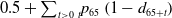
Many OECD nations are raising their retirement age threshold to 67 years or higher (Hammond et al., Reference Hammond, Baxter, Bramley, Kakkad, Mehta and Sadler2016). They have tied future prospective retirement age adjustments to anticipated changes in life expectancy. While this approach is convenient and reasonable, focusing solely on life expectancy does not cover the whole picture. Greater emphasis should be placed on estimating the duration for which individuals can maintain full working capacity. Healthy life expectancy serves as a valuable measure for assessing this duration. It is generally defined as the average number of years a person is expected to live in good health, free from significant illness or disability, based on the mortality and health conditions in a calendar year. Figure 3 shows the life expectancy and healthy life expectancy trends of Australian females and males aged 65 years. Following the rationale in Jagger et al. (Reference Jagger, Cox and Le Roy2006), we calculate the (period) life expectancy values as $0.5 + \mathop \sum \nolimits_{t \gt 0} {}_t^{}{p_{65}}$
and the (period) healthy life expectancy values as
$0.5 + \mathop \sum \nolimits_{t \gt 0} {}_t^{}{p_{65}}$
and the (period) healthy life expectancy values as $0.5 + \mathop \sum \nolimits_{t \gt 0} {}_t^{}{p_{65}}\left( {1 - {d_{65 + t}}} \right)$
, in which
$0.5 + \mathop \sum \nolimits_{t \gt 0} {}_t^{}{p_{65}}\left( {1 - {d_{65 + t}}} \right)$
, in which ${}_t^{}{p_{65}}$
is the probability of survival at time t of a person aged 65 years at time 0 and
${}_t^{}{p_{65}}$
is the probability of survival at time t of a person aged 65 years at time 0 and ${d_{65 + t}}$
is the corresponding prevalence rate. It can be seen in Figure 3 that there is a clear gap between the two measures, being about 5.5 years for females and 3.4 years for males on average. As of 2018, female (male) life expectancy at age 65 years is 22.9 (20.2) years, while healthy life expectancy at age 65 years is 17.5 (16.8) years. The expected durations spent in healthy and unhealthy statuses have important implications for health and retirement issues.
${d_{65 + t}}$
is the corresponding prevalence rate. It can be seen in Figure 3 that there is a clear gap between the two measures, being about 5.5 years for females and 3.4 years for males on average. As of 2018, female (male) life expectancy at age 65 years is 22.9 (20.2) years, while healthy life expectancy at age 65 years is 17.5 (16.8) years. The expected durations spent in healthy and unhealthy statuses have important implications for health and retirement issues.
Life expectancy (dashed) and healthy life expectancy (solid) values at age 65 years for both sexes in Australia from 1990 to 2021.

3. Bayesian modelling
We propose the following multi-population framework for modelling the disability prevalence rates for both sexes jointly. First, the log prevalence rate is assumed as:
 \begin{align*}{\rm{log}}( {{d_{s,x,t}}} ) = {\mu _{s,x,t}} + {e_{s,x,t}}, \end{align*}
where ${d_{s,x,t}}$
is the prevalence rate at age x in year t of sex s,
${d_{s,x,t}}$
is the prevalence rate at age x in year t of sex s, ${\mu _{s,x,t}}$
is the corresponding mean structure, and
${\mu _{s,x,t}}$
is the corresponding mean structure, and ${e_{s,x,t}}$
is the normal error term with mean zero and variance
${e_{s,x,t}}$
is the normal error term with mean zero and variance $\sigma _s^2$
. We experiment with a number of different mean structures, the first set of which has a common factor for both sexes and a certain number of sex-specific factors (Li and Lee, Reference Li and Lee2005; Li, Reference Li2013), denoted as CFMn here:
$\sigma _s^2$
. We experiment with a number of different mean structures, the first set of which has a common factor for both sexes and a certain number of sex-specific factors (Li and Lee, Reference Li and Lee2005; Li, Reference Li2013), denoted as CFMn here:
 \begin{align*}{\mu _{s,x,t}} = {a_{s,x}} + {B_x}{K_t} + \mathop \sum \nolimits_{j = 1}^n {b_{s,x,j}}{k_{s,t,j}}, \end{align*}
in which ${a_{s,x}}$
describes the disability prevalence profile over age of sex s,
${a_{s,x}}$
describes the disability prevalence profile over age of sex s, ${B_x}{K_t}$
is the common factor for females and males, and
${B_x}{K_t}$
is the common factor for females and males, and ${b_{s,x,j}}{k_{s,t,j}}$
is the jth specific factor of sex s (with a total of n specific factors). The common factor depicts the major long-term trend in disability prevalence for the whole population. The sex-specific factor represents the short-term deviation from the major trend for each sex. The parameters
${b_{s,x,j}}{k_{s,t,j}}$
is the jth specific factor of sex s (with a total of n specific factors). The common factor depicts the major long-term trend in disability prevalence for the whole population. The sex-specific factor represents the short-term deviation from the major trend for each sex. The parameters ${B_x}$
and
${B_x}$
and ${b_{s,x,j}}$
refer to the sensitivity of the log prevalence rate to the time series
${b_{s,x,j}}$
refer to the sensitivity of the log prevalence rate to the time series ${K_t}$
and
${K_t}$
and ${k_{s,t,j}}$
.Footnote
5
This mean structure reduces to the classical Lee–Carter method (for modelling mortality rates) if the common factor is omitted and if there is only one specific factor.
${k_{s,t,j}}$
.Footnote
5
This mean structure reduces to the classical Lee–Carter method (for modelling mortality rates) if the common factor is omitted and if there is only one specific factor.
Moreover, we consider two modified versions which are more parsimonious. The first one has only one additional factor, where ${b_x}$
is shared by both sexes (denoted as MI):
${b_x}$
is shared by both sexes (denoted as MI):
 \begin{align*}{\mu _{s,x,t}} = {a_{s,x}} + {B_x}{K_t} + {b_x}{k_{s,t}}. \end{align*}
The second one further constrains all the sensitivities to ${B_x}$
only (denoted as MII):
${B_x}$
only (denoted as MII):
 \begin{align*}{\mu _{s,x,t}} = {a_{s,x}} + {B_x}{K_t} + {B_x}{k_{s,t}}. \end{align*}
The deviance information criterion (DIC) is adopted here to choose the optimal structure. The DIC is designed for Bayesian analysis and is calculated as $D\left( {\bar \theta } \right) + 2{p_D}$
, where
$D\left( {\bar \theta } \right) + 2{p_D}$
, where $D\left( {\bar \theta } \right)$
is the deviance value, using the posterior mean
$D\left( {\bar \theta } \right)$
is the deviance value, using the posterior mean ${\bar \theta }$
, and
${\bar \theta }$
, and ${p_D}$
is the effective number of parameters (Spiegelhalter et al., Reference Spiegelhalter, Thomas, Best and Lunn2003) under the Bayesian context. It effectively allows for both the goodness-of-fit and parameter parsimony. A lower DIC value generally indicates a better model structure.
${p_D}$
is the effective number of parameters (Spiegelhalter et al., Reference Spiegelhalter, Thomas, Best and Lunn2003) under the Bayesian context. It effectively allows for both the goodness-of-fit and parameter parsimony. A lower DIC value generally indicates a better model structure.
Figure 1 shows that the log prevalence rates at different age groups decrease rather linearly over the period. Accordingly, we assume that ${K_t}$
follows a random walk with drift as
${K_t}$
follows a random walk with drift as ${K_t} = \;\vartheta + {K_{t - 1}} + {\varepsilon _t}$
, where
${K_t} = \;\vartheta + {K_{t - 1}} + {\varepsilon _t}$
, where $\vartheta $
is the drift term and
$\vartheta $
is the drift term and ${\varepsilon _t}\sim {\rm{Normal}}( {0,\sigma _K^2} )$
. Moreover, the short-term discrepancy from the major trend for each sex is supposed to fade out over time. We then assume that
${\varepsilon _t}\sim {\rm{Normal}}( {0,\sigma _K^2} )$
. Moreover, the short-term discrepancy from the major trend for each sex is supposed to fade out over time. We then assume that ${k_{s,t,j}}$
follows an AR(1) process as
${k_{s,t,j}}$
follows an AR(1) process as ${k_{s,t,j}} = \;{\alpha _{s,0,j}} + {\alpha _{s,1,j}}{k_{s,t - 1,j}} + {\varepsilon _{s,t,j}}$
, in which
${k_{s,t,j}} = \;{\alpha _{s,0,j}} + {\alpha _{s,1,j}}{k_{s,t - 1,j}} + {\varepsilon _{s,t,j}}$
, in which ${\alpha _{s,0,j}}$
is the intercept,
${\alpha _{s,0,j}}$
is the intercept, ${\alpha _{s,1,j}}$
is the autoregressive parameter, and
${\alpha _{s,1,j}}$
is the autoregressive parameter, and ${\varepsilon _{s,t,j}}\sim{\rm{Normal}}\left( {0,\sigma _{k,s,j}^2} \right)$
. When the AR(1) process is weakly stationary (
${\varepsilon _{s,t,j}}\sim{\rm{Normal}}\left( {0,\sigma _{k,s,j}^2} \right)$
. When the AR(1) process is weakly stationary ( $\left| {{\alpha _{s,1,j}}} \right| \lt 1$
), the forecast value of
$\left| {{\alpha _{s,1,j}}} \right| \lt 1$
), the forecast value of ${k_{s,t,j}}$
converges to a constant, and so the deviation from the main trend diminishes. This treatment prevents the female and male prevalence rates from diverging from each other indefinitely. Note also that there are only 5 years of disability prevalence data available, which are separated by time periods of different lengths, so the time series processes assumed are reasonable choices under these data limitations.
${k_{s,t,j}}$
converges to a constant, and so the deviation from the main trend diminishes. This treatment prevents the female and male prevalence rates from diverging from each other indefinitely. Note also that there are only 5 years of disability prevalence data available, which are separated by time periods of different lengths, so the time series processes assumed are reasonable choices under these data limitations.
The posterior distribution of the unknown parameters is derived as f(θ|D) ∝ f(D|θ) f(θ) (i.e., likelihood × prior). The predictive distribution of the variables of interest is then derived as f(x|D) = ∫ f(x|θ) f(θ|D) dθ (i.e., integrating process distribution × posterior distribution). For our proposed framework, however, a close-formed solution of the posterior and predictive distributions cannot be obtained. The MCMC simulation process can address this issue by approximating the joint posterior distribution. Specifically, the MCMC process simulates from a Markov chain which has a stationary distribution equivalent to the posterior distribution. The software WinBUGS adopts the Gibbs sampling method, simulating sequentially from the full conditional posterior distribution of each variable. This software is chosen because it is well suited for Bayesian MCMC, facilitating model specification, efficient handling of missing data and latent variables, and robust convergence diagnostics. It is widely used in demographic and actuarial studies (e.g., Li, Reference Li2014), providing both reliability and comparability with existing literature. The priors of ${a_{s,x}}$
,
${a_{s,x}}$
, ${B_x}$
, and
${B_x}$
, and ${b_{s,x,j}}$
are set as normal. The time series parameters
${b_{s,x,j}}$
are set as normal. The time series parameters $\vartheta $
,
$\vartheta $
, ${\alpha _{s,0,j}}$
, and
${\alpha _{s,0,j}}$
, and $\;{\alpha _{s,1,j}}$
are also assumed to be normally distributed. The variances
$\;{\alpha _{s,1,j}}$
are also assumed to be normally distributed. The variances $\sigma _s^2$
,
$\sigma _s^2$
, $\sigma _K^2$
, and
$\sigma _K^2$
, and $\sigma _{k,s,\,j}^2$
are treated as following the inverse gamma distribution. More information is provided in the Appendix.
$\sigma _{k,s,\,j}^2$
are treated as following the inverse gamma distribution. More information is provided in the Appendix.
DIC values of different prevalence model structures (with rankings in brackets).

Table 1 reports the DIC values of different model structures. The common factor models with zero, one, and two specific factors are referred to as CFM0, CFM1, and CFM2, respectively. The two modified versions are termed as MI and MII. The MI model gives the lowest DIC value, and the CFM0 model has the second lowest. Adding more factors to the CFM0 does not necessarily decrease the DIC value, as using too many parameters is penalised in the DIC computation. Accordingly, we use the MI model for all the analyses below. As shown in the Appendix, the heatmaps of the residuals show no discernible patterns, further indicating that the MI model provides a reasonable fit to the prevalence data.
Parameter estimates (posterior means) of MI prevalence model.

Figure 4 displays the parameter estimates (posterior means) of the MI model. The overall disability prevalence profile ( ${a_{s,x}}$
) has an increasing pattern with age for both sexes, in which the female prevalence rates are higher than the male rates. The major time-varying parameter (
${a_{s,x}}$
) has an increasing pattern with age for both sexes, in which the female prevalence rates are higher than the male rates. The major time-varying parameter ( ${K_t}$
) of the common factor demonstrates clearly a linearly declining trend. Its sensitivity (
${K_t}$
) of the common factor demonstrates clearly a linearly declining trend. Its sensitivity ( ${B_x}$
) fluctuates over age but tends to be lower for the older age groups. Moreover, the time-varying parameters (
${B_x}$
) fluctuates over age but tends to be lower for the older age groups. Moreover, the time-varying parameters ( ${k_{s,t}}$
) of the additional factor for females and males do not show any clear trends, though there may be some mild decrease in the more recent years for females. Their sensitivity (
${k_{s,t}}$
) of the additional factor for females and males do not show any clear trends, though there may be some mild decrease in the more recent years for females. Their sensitivity ( ${b_x}$
) does not seem to have a strong age pattern, yet it tends to be higher for the younger age groups. Table 2 provides the parameter estimates of the time series parameters and (inverse) variance terms. The negative value of the drift term (
${b_x}$
) does not seem to have a strong age pattern, yet it tends to be higher for the younger age groups. Table 2 provides the parameter estimates of the time series parameters and (inverse) variance terms. The negative value of the drift term ( $\vartheta $
) indicates that the disability prevalence rates decline generally over time. The autoregressive parameters (
$\vartheta $
) indicates that the disability prevalence rates decline generally over time. The autoregressive parameters ( ${\alpha _{s,1}}$
) are way smaller than one in magnitude, revealing that the forecast female and male prevalence rates will not diverge in the long term.
${\alpha _{s,1}}$
) are way smaller than one in magnitude, revealing that the forecast female and male prevalence rates will not diverge in the long term.
Parameter estimates (posterior means) of MI prevalence model.

Figure 5 plots the observed and imputed log prevalence rates from 2003 to 2018 and the forecasted rates from 2019 to 2060, alongside the Bayesian 95% probability intervals. The mean forecasts tend to decline faster over time for the younger age groups, broadly in line with the sensitivity estimates as discussed earlier, while the prediction intervals are wider and so there is more uncertainty for the older age groups. These forecasted and simulated values can be integrated with those of the mortality rates to estimate future healthy life expectancy and valuate retirement village contracts. (As a sensitivity check, we also apply the MI model to the combined data of profound, severe, moderate, and mild disability. As demonstrated in the Appendix, the overall time trends and forecast uncertainty are broadly in line with those from focusing on profound and severe disability.)
Observed and forecasted log prevalence rates with 95% probability intervals from 2003 to 2060 for both sexes under MI prevalence model.

Furthermore, we conduct two out-of-sample tests by fitting the MI model to the data of 2003–2012 and 2003–2015 and forecasting 2015 and 2018, respectively. The resulting mean absolute percentage errors of the 2015 and 2018 forecasted log prevalence rates over both sexes and all age groups are only 6.9% and 6.0%, both within an acceptable range. The observed rates also lie comfortably within the 95% prediction intervals. These results indicate that the MI model performs reasonably well despite the limited data.
We then adopt the same multi-population framework for modelling the death rates ( ${m_{s,x,t}}$
at age x in year t of sex s) for both sexes, including the CFMn, MI, and MII models. Table 3 compares the DIC values of different mortality model structures. The CFM2 model gives the lowest DIC value, the result of which is in line with Li (Reference Li2013) on Australian mortality. While incorporating more factors can decrease the DIC value here, there appears to be a limit on how far it can be improved, as parameter parsimony is allowed for in the DIC. In the following, we then use the CFM2 model for forecasting and simulating the mortality rates. Figure 6 exhibits the observed and forecasted log death rates from 1980 to 2060 and the corresponding 95% prediction intervals. Based on the simulation results, the mortality rates are expected to continue to decline in the next few decades, with some extent of uncertainty at different ages.
${m_{s,x,t}}$
at age x in year t of sex s) for both sexes, including the CFMn, MI, and MII models. Table 3 compares the DIC values of different mortality model structures. The CFM2 model gives the lowest DIC value, the result of which is in line with Li (Reference Li2013) on Australian mortality. While incorporating more factors can decrease the DIC value here, there appears to be a limit on how far it can be improved, as parameter parsimony is allowed for in the DIC. In the following, we then use the CFM2 model for forecasting and simulating the mortality rates. Figure 6 exhibits the observed and forecasted log death rates from 1980 to 2060 and the corresponding 95% prediction intervals. Based on the simulation results, the mortality rates are expected to continue to decline in the next few decades, with some extent of uncertainty at different ages.
DIC values of different mortality model structures (with rankings in brackets).

Observed and forecasted log death rates with 95% prediction intervals from 1980 to 2060 for both sexes under CFM2 mortality model.

Regarding the economic and financial variables for valuing a retirement village contract in Section 4, the residential property price index and consumer price index (CPI) quarterly data are collected from the Australian Bureau of Statistics (ABS)Footnote 6 for a 20-year period of 2005–2024. The corresponding 3-month bank accepted bills monthly yields are obtained from the Reserve Bank of Australia (RBA).Footnote 7 Figure 7 shows that the Australian property market has experienced substantial growth over the period, with some cyclical fluctuations. The quarterly growth rate of property values varies between −3.00% and 6.70%. Moreover, both inflation and interest rates exhibit cyclical patterns. The quarterly inflation rate fluctuates between −1.89% and 2.14%, while the quarterly interest rate moves between 0.00% and 1.95%.
For modelling the interest rate ( ${r_{t,1}}$
), we consider using the Cox–Ingersoll–Ross (CIR) model as follows:
${r_{t,1}}$
), we consider using the Cox–Ingersoll–Ross (CIR) model as follows:
 \begin{align*}d{r_{t,1}} = {a_1}({{b_1} - {r_{t,1}}}) dt + {\sigma _1}\sqrt {{r_{t,1}}} d{W_{t,1}}, \end{align*}
where ${r_t}$
is the rate at time t,
${r_t}$
is the rate at time t, $a$
(> 0) is the pace of adjustment to the mean
$a$
(> 0) is the pace of adjustment to the mean $b$
,
$b$
, $\sigma $
(> 0) is the volatility,
$\sigma $
(> 0) is the volatility, ${W_t}$
is the Wiener process, and the subscript (1) refers to the interest rate. This model ensures mean reversion of the interest rate and avoids the possibility of negative values. For modelling the inflation and property growth rates (
${W_t}$
is the Wiener process, and the subscript (1) refers to the interest rate. This model ensures mean reversion of the interest rate and avoids the possibility of negative values. For modelling the inflation and property growth rates ( ${r_{t,2}}$
,
${r_{t,2}}$
, ${r_{t,3}}$
), we consider adopting the Ornstein–Uhlenbeck (OU) model as below:
${r_{t,3}}$
), we consider adopting the Ornstein–Uhlenbeck (OU) model as below:
 \begin{align*}d{r_{t,2}} = {a_2}( {{b_2} - {r_{t,2}}}) dt + {\sigma _2}d{W_{t,2}}, \\[-25pt] \end{align*}
 \begin{align*}d{r_{t,3}} = {a_3}( {{b_3} - {r_{t,3}}}) dt + {\sigma _3}d{W_{t,3}}, \end{align*}
in which the parameters have the same meanings as those above. This model also has mean reversion, but it allows both positive and negative values. For both the CIR and OU models, the stochastic term $\sigma d{W_t}$
introduces normally distributed shocks. The Euler–Maruyama approximation method is used to cope with the discrete nature of the time series. Under the Bayesian framework, the priors of
$\sigma d{W_t}$
introduces normally distributed shocks. The Euler–Maruyama approximation method is used to cope with the discrete nature of the time series. Under the Bayesian framework, the priors of $a$
and
$a$
and $b$
are set as truncated normal and normal, and the prior of
$b$
are set as truncated normal and normal, and the prior of ${\sigma ^2}$
is set as inverse gamma. The priors of the correlation coefficients between the normally distributed shocks are assumed to be uniform.
${\sigma ^2}$
is set as inverse gamma. The priors of the correlation coefficients between the normally distributed shocks are assumed to be uniform.
Note that we use the residential property price index as a proxy, although in reality each retirement village is unique. We suppose that the price movements across all properties within the retirement village portfolio are homogeneous. Moreover, we assume that demographic risks and market risks are independent. Table 4 lists the parameter estimates of the CIR and OU models. The estimates of ${b_1}$
,
${b_1}$
, ${b_2}$
, and
${b_2}$
, and ${b_3}$
are fairly close to the sample means of the interest, inflation, and property growth rates across the period. The estimated values of
${b_3}$
are fairly close to the sample means of the interest, inflation, and property growth rates across the period. The estimated values of ${a_1}$
,
${a_1}$
, ${a_2}$
, and
${a_2}$
, and ${a_3}$
indicate different rates of mean reversion. There is a relatively high estimated correlation (
${a_3}$
indicate different rates of mean reversion. There is a relatively high estimated correlation ( ${\rho _{12}}$
) between the stochastic processes of the interest and inflation rates. Figure 8 demonstrates that the simulated distributions of the three quarterly rates align reasonably well with the historical data.
${\rho _{12}}$
) between the stochastic processes of the interest and inflation rates. Figure 8 demonstrates that the simulated distributions of the three quarterly rates align reasonably well with the historical data.
Parameter estimates (posterior means) of CIR and OU models.

Australian quarterly residential property price index values (left) and quarterly property growth rates, inflation rates, and interest rates (right) from 2005 to 2024.

Simulated distributions of Australian quarterly interest, inflation, and property growth rates.

4. Retirement village
In recent years, retirement villages have become an increasingly popular housing choice for older Australians, particularly those facing financial challenges due to being “asset rich but cash poor.” They are primarily designed for individuals who can manage independent living but prefer the convenience, security, and social interaction of a community-based environment (Kyng et al., Reference Kyng, Pitt, Purcal and Zhang2021). The majority of residents are well into their seventies, and entry is typically restricted to those aged 55 years and above. These villages offer a range of accommodation options, each providing a mix of services and on-site facilities tailored to older individuals. Nevertheless, retirement villages are not equipped to provide intensive care and are not a substitute for nursing homes or specialised aged care facilities. Under the contract terms, residents are typically required to relocate to an aged care facility if they become unable to manage essential day-to-day tasks independently. Figure 9 illustrates the different stages of a retiree’s life and summarises the key considerations and factors in transitions between stages. Common reasons for moving into retirement villages include financial constraints, feeling of loneliness, social isolation, downsizing after children have moved out, the appeal of communal lifestyle, and access to age-friendly services and facilities. Over the past five years, industry revenue in this market has grown at an average annual rate of 2.3%, reaching (AUD) $6.1 billion in 2024.Footnote 8 Currently, close to 10% of Australians aged 65 years and older reside in retirement villages, indicating considerable potential for future growth. The Appendix provides a list of the major retirement village providers in Australia.
Different stages of residence of an Australian retiree and underlying considerations and factors.

Retirement village contracts are diverse and often feature intricate financial arrangements. According to Kyng et al. (Reference Kyng, Pitt, Purcal and Zhang2021), these contracts typically share several key financial components. To begin with, residents are required to pay an upfront entry fee ( ${P_0}$
), usually as a lump sum. This payment secures the right to occupy a unit within the village. The right ceases upon the resident’s passing, inability to live independently, or relocation to another place in other circumstances. Often, residents fund this initial payment using a portion of the proceeds from selling their original family homes. Notably, the entry fee is generally more affordable than purchasing a comparable non-retirement property within the same residential area, making it a financially attractive option for many seniors. For instance, in 2021, the national average entry fee for a two-bedroom unit in a retirement village was $484,000,Footnote
9
while the average unit price in Australia was $601,000.Footnote
10
Moreover, when residing in the retirement village, the resident typically contributes a regular maintenance fee. This ongoing fee covers shared expenses such as facility upkeep, utilities for communal areas, staffing, and the provision of general services. It is usually set on a cost-recovery basis rather than being structured to generate profit for the operator. In 2021, the average monthly maintenance fee was $502.Footnote
11
This type of fee can be adjusted with inflation over time.
${P_0}$
), usually as a lump sum. This payment secures the right to occupy a unit within the village. The right ceases upon the resident’s passing, inability to live independently, or relocation to another place in other circumstances. Often, residents fund this initial payment using a portion of the proceeds from selling their original family homes. Notably, the entry fee is generally more affordable than purchasing a comparable non-retirement property within the same residential area, making it a financially attractive option for many seniors. For instance, in 2021, the national average entry fee for a two-bedroom unit in a retirement village was $484,000,Footnote
9
while the average unit price in Australia was $601,000.Footnote
10
Moreover, when residing in the retirement village, the resident typically contributes a regular maintenance fee. This ongoing fee covers shared expenses such as facility upkeep, utilities for communal areas, staffing, and the provision of general services. It is usually set on a cost-recovery basis rather than being structured to generate profit for the operator. In 2021, the average monthly maintenance fee was $502.Footnote
11
This type of fee can be adjusted with inflation over time.
When departing the retirement village, the leaving resident is refunded the entry fee minus any applicable exit fees by the operator. One standard type of exit fee is the deferred management fee, which is equal to a prespecified percentage ( $fee$
) of the entry fee times the duration of residence. The total amount of this exit fee is often capped at a certain limit (
$fee$
) of the entry fee times the duration of residence. The total amount of this exit fee is often capped at a certain limit ( $cap$
). The typical upper limit is around 30%, where it usually takes between 5 and 10 years of residence to reach this level. The deferred management fee, calculated as
$cap$
). The typical upper limit is around 30%, where it usually takes between 5 and 10 years of residence to reach this level. The deferred management fee, calculated as ${P_0}\; \times \min \left( {fee \times t\;,\;cap} \right)$
when departure occurs in year t, serves as one primary source of profit for the operator. Furthermore, a retirement village contract may contain a provision for the resident to share a proportion (
${P_0}\; \times \min \left( {fee \times t\;,\;cap} \right)$
when departure occurs in year t, serves as one primary source of profit for the operator. Furthermore, a retirement village contract may contain a provision for the resident to share a proportion ( $share$
) of the capital gain/loss. The change in capital is calculated as
$share$
) of the capital gain/loss. The change in capital is calculated as $\left( {{P_t} - {P_0}} \right)$
, that is, the entry fee paid by the new resident minus the entry fee originally paid by the leaving resident. The shared capital/loss is then computed as
$\left( {{P_t} - {P_0}} \right)$
, that is, the entry fee paid by the new resident minus the entry fee originally paid by the leaving resident. The shared capital/loss is then computed as $\left( {{P_t} - {P_0}} \right) \times share$
. Other potential costs, such as those associated with renovations and refurbishments, may also be included. All the key financial components of retirement village contracts are summarised in Figure 10. Upon departure, the net cash flow for the operator can be expressed as
$\left( {{P_t} - {P_0}} \right) \times share$
. Other potential costs, such as those associated with renovations and refurbishments, may also be included. All the key financial components of retirement village contracts are summarised in Figure 10. Upon departure, the net cash flow for the operator can be expressed as $\left( {{P_0}\; \times \min \left( {fee \times t\;,\;cap} \right) - {P_0} - \left( {{P_t} - {P_0}} \right) \times share} \right)$
, in which there is a refund of
$\left( {{P_0}\; \times \min \left( {fee \times t\;,\;cap} \right) - {P_0} - \left( {{P_t} - {P_0}} \right) \times share} \right)$
, in which there is a refund of ${P_0}$
to the leaving resident. It is assumed that the regular maintenance fee covers exactly the actual maintenance costs and so this component cancels out and does not appear in the cash flow equation.
${P_0}$
to the leaving resident. It is assumed that the regular maintenance fee covers exactly the actual maintenance costs and so this component cancels out and does not appear in the cash flow equation.
Basic retirement village contract structure.

The payments under a retirement village contract depend on uncertain factors such as morbidity, mortality, and housing prices. Within the proposed Bayesian framework in Section 3, we model these random processes explicitly to estimate the cash flows. Conceptually, the contract’s features can be compared to familiar financial instruments: ongoing maintenance fees behave like a life annuity, the exit refund resembles a life and health cover with variable benefits, and the sharing of property value changes parallels an option or forward on real estate.
A related financial arrangement that can be used as a benchmark for comparison is a reverse mortgage (e.g., Kogure et al., Reference Kogure, Li and Kamiya2014), which also combines several financial components within a single contract. Under a reverse mortgage, an individual borrows against the equity of their home while continuing to reside in the property, and the loan balance accrues interest over time. The repayment is made when the borrower leaves the property due to death or other reasons. The proceeds from the home sale are used to settle the outstanding loan. There is generally a nonrecourse provision, in which the borrower’s obligation to repay the loan is capped at the value of the property. This feature is equivalent to the borrower holding a put option on the property, with its strike price equal to the loan balance. In a similar vein, the payments under a reverse mortgage depend on uncertain factors including mortality, health status, property values, and interest rates. Compared to a retirement village contract, a reverse mortgage offers greater liquidity to the customer because of the upfront loan, while likewise it does not bundle accommodation with guaranteed access to on-site long-term careFootnote 12 . On the other hand, taking a reverse mortgage means that the individual continues living independently and does not benefit from the community life and services offered in a retirement village. While the non-pecuniary benefits (e.g., community lifestyle, social support) are difficult to quantify, they would represent a significant source of value for retirement village residents and it should not be understated.
Non-pecuniary benefits such as community belonging, social interaction, and perceived security are fundamentally subjective and vary considerably across individuals. Unlike financial cash flows, they do not have directly observable market prices. Although direct monetary valuation is challenging, empirical evidence shows that residing within a social community is associated with higher subjective well-being among older adults relative to living alone, and that greater social capital predicts better quality of life outcomes. Lee et al. (Reference Lee, Huang, Wu, Yeh and Chang2023) report that ageing in the community significantly increases the odds of higher subjective well-being by about seven times. Hao and Chen (Reference Hao and Chen2026) find that the correlations between social capital and well-being are in the range of 0.70. Gao et al. (Reference Gao, Ho, Chua and Feng2024) combine qualitative and geographic information systems methods and highlight that structured social networks and access to community spaces are identified as important components of well-being in later life. These findings indicate that community-based social environments may generate economically meaningful welfare benefits.
We now consider a typical retirement village contract as a base-case scenario for our study. Under Australian market conventions, the contract terms are not influenced by the age or sex of the resident. We evaluate this contract from the perspective of an Australian operator. Consider that an individual aged 61–80 years in 2025 is offered an entry fee of $600,000. The contract terms include a maintenance fee of $8,000 per annum (subject to inflation adjustments), a deferred management fee of 6% per annum (with an upper limit of 18%, 30%, or 42% on the total fee), and an entitlement to 10%, 30%, or 50% of any capital gain (or loss) upon departure. The net refund for the leaving resident is calculated as $\left( {{P_0} + \left( {{P_t} - {P_0}} \right) \times share - {P_0}\; \times \min \left( {fee \times t\;,\;cap} \right)} \right)$
, that is, the entry fee plus the capital gain shared minus the deferred management fee. These settings are broadly in line with the current market conditions.Footnote
13
$\left( {{P_0} + \left( {{P_t} - {P_0}} \right) \times share - {P_0}\; \times \min \left( {fee \times t\;,\;cap} \right)} \right)$
, that is, the entry fee plus the capital gain shared minus the deferred management fee. These settings are broadly in line with the current market conditions.Footnote
13
Our analysis considers only involuntary exits caused by disability or death, excluding voluntary departures arising from personal or financial circumstances. The modelling framework incorporates both systematic morbidity and longevity risks. However, we assume a homogenous retirement village portfolio of sufficiently large size, minimising the impact of non-systematic morbidity and longevity risks (i.e., individual idiosyncrasies). Accordingly, the uncertainty of future outcomes in our settings is driven by systematic risks in morbidity, mortality, and properties, rather than non-systematic risks.
For each of the 1,000 scenarios simulated from the Bayesian framework in Section 3, the average net cash flow in year t for the operator under this retirement village contract within a homogenous portfolio is computed as (for t = 1, 2, …):
 \begin{align*}C{F_t} &= \left( {{P_0}\; \times \min \left( {fee \times t\;,\;cap} \right) - {P_0} - \left( {{P_t} - {P_0}} \right) \times share} \right) \\[4pt] &\quad\times ({{}_t^{}{p_{s,x}}( {\;{d_{s,x + t,t}} - \;{d_{s,x + t - 1,t - 1}}}) + {}_{t - 1}^{}{p_{s,x}}( {1 - \;{d_{s,x + t - 1,t - 1}}} )( {1 - {p_{s,x + t - 1}}})} )/( {1 - \;{d_{s,x,0}}}), \end{align*}
where ${P_0}$
is the entry fee,
${P_0}$
is the entry fee, $fee$
is the deferred management fee per annum,
$fee$
is the deferred management fee per annum, $cap$
is the upper limit on its total amount,
$cap$
is the upper limit on its total amount, $share$
is the proportion of capital gain or loss (
$share$
is the proportion of capital gain or loss ( ${P_t} - {P_0} = {P_0}\mathop \prod \nolimits_{u = 1}^t ( {1 + {r_{u,3}}} ) - {P_0}$
) offered to the departing resident, and
${P_t} - {P_0} = {P_0}\mathop \prod \nolimits_{u = 1}^t ( {1 + {r_{u,3}}} ) - {P_0}$
) offered to the departing resident, and ${r_{t,3}}$
is the annual property growth rate from time t – 1 to time t. The term
${r_{t,3}}$
is the annual property growth rate from time t – 1 to time t. The term ${}_t^{}{p_{s,x}} = \mathop \prod \nolimits_{u = 1}^t {\rm{exp}}( { - {m_{s,x + u - 1,u}}} )$
is the (cohort) probability of survival in year t for an individual aged x of sex s at the time of entry, and
${}_t^{}{p_{s,x}} = \mathop \prod \nolimits_{u = 1}^t {\rm{exp}}( { - {m_{s,x + u - 1,u}}} )$
is the (cohort) probability of survival in year t for an individual aged x of sex s at the time of entry, and ${d_{s,x + t,t}}$
is the corresponding prevalence rate in year t. In effect,
${d_{s,x + t,t}}$
is the corresponding prevalence rate in year t. In effect, ${}_t^{}{p_{s,x}}( {\;{d_{s,x + t,t}} - \;{d_{s,x + t - 1,t - 1}}} )/( {1 - \;{d_{s,x,0}}} )$
refers to the proportion of becoming disabled in year t, and
${}_t^{}{p_{s,x}}( {\;{d_{s,x + t,t}} - \;{d_{s,x + t - 1,t - 1}}} )/( {1 - \;{d_{s,x,0}}} )$
refers to the proportion of becoming disabled in year t, and ${}_{t - 1}^{}{p_{s,x}}( {1 - \;{d_{s,x + t - 1,t - 1}}} )( {1 - {p_{s,x + t - 1}}} )/( {1 - \;{d_{s,x,0}}} )$
refers to the proportion of healthy lives dying in year t. The denominator
${}_{t - 1}^{}{p_{s,x}}( {1 - \;{d_{s,x + t - 1,t - 1}}} )( {1 - {p_{s,x + t - 1}}} )/( {1 - \;{d_{s,x,0}}} )$
refers to the proportion of healthy lives dying in year t. The denominator $1 - \;{d_{s,x,0}}$
makes it a conditional probability and allows for the fact that the new resident is supposed to be reasonably healthy at the time of entry (time 0).
$1 - \;{d_{s,x,0}}$
makes it a conditional probability and allows for the fact that the new resident is supposed to be reasonably healthy at the time of entry (time 0).
Compared to Li (Reference Li2024a), who uses healthy life expectancy as a proxy for the length of stay and focused on entry at the age of 60 years only, our modelling approach here is much more precise and flexible for different entry ages, making good use of the underlying morbidity trends in the data, rather than relying on indirect information from a rigid summary metric. Moreover, Li (Reference Li2024a) uses period healthy life expectancy values, each of which was calculated from the prevalence and mortality rates in a single calendar year and did not allow for the real possible developments of each cohort over time. By contrast, we utilise cohort-specific probabilities of survival, death, and prevalence in computing the cash flows. This method is more realistic and relevant for accurately valuing a retirement village contract. Furthermore, we make use of conditional probabilities, allowing for the assumption that the new resident can live independently at the start. But the healthy life expectancy approach in Li (Reference Li2024a) does not take this condition into account explicitly.
While the data sources and the underlying disability definitions are significantly different between this study and Li (Reference Li2024a), some interesting observations can be made when comparing their widths of prediction intervals and general levels of uncertainty allowed. Under our modelling approach, the width of 95% prediction intervals increases from a few percents of the mean to 10 per cents or more for a forecast period of (say) 30 years. This degree of widening is reasonable, as it reflects the compounding uncertainty over time from modelling the underlying rates. By contrast, the level of uncertainty allowed in Li (Reference Li2024) is driven mainly by the ARIMA order chosen for life expectancy when co-modelling life expectancy and healthy life expectancy. A higher selected ARIMA order would lead to wider prediction intervals due to increased parameter uncertainty. As a result, the level of uncertainty allowed can be quite uneven between both sexes within a country or between neighbouring countries when their ARIMA orders are different. In comparison, our modelling approach provides more stable and reasonable prediction intervals in general.
The EPV at time 0 of all the cash flows under the retirement village contract is then calculated as ${\rm{E}}[ {\mathop \sum \nolimits_{t = 1}^{\omega - x} ( {C{F_t}/{{1.1}^t}} )} ] + {P_0}$
, in which the discount rate is taken as 10% per annum and
${\rm{E}}[ {\mathop \sum \nolimits_{t = 1}^{\omega - x} ( {C{F_t}/{{1.1}^t}} )} ] + {P_0}$
, in which the discount rate is taken as 10% per annum and $\omega $
is the limiting age of the new resident.Footnote
14
The assumed discount rate is based on the fact that the average total return of Australian residential property is about 10% per annum for the past decade,Footnote
15
and generally speaking, its exceedance over the risk-free rate reflects the market compensation for assuming property-related risks. Note that the net cash flows at t = 1, 2, … are generally negative for the operator, while the EPV at time 0 becomes positive mainly because of the entry fee
$\omega $
is the limiting age of the new resident.Footnote
14
The assumed discount rate is based on the fact that the average total return of Australian residential property is about 10% per annum for the past decade,Footnote
15
and generally speaking, its exceedance over the risk-free rate reflects the market compensation for assuming property-related risks. Note that the net cash flows at t = 1, 2, … are generally negative for the operator, while the EPV at time 0 becomes positive mainly because of the entry fee ${P_0}$
received at time 0.
${P_0}$
received at time 0.
Using the MCMC simulated values of the cash flows, Figure 11 illustrates the EPVs (which are effectively the profits for the operator) for a range of cases when the deferred management fee cap is 30%. First, there are significant differences in the profits between different levels of capital gain sharing. The profits decrease by around $40,000 to $50,000 from 10% to 30% sharing increase and from 30% to 50% sharing, indicating approximately a 5% drop in profit for every 10% increase in capital gain sharing. Second, the profits are lower when the residents move into the retirement village at older ages. Higher entry ages are associated with higher prevalence and mortality rates, resulting in shorter expected lengths of stay. Consequently, the entry fee is refunded sooner, with less discounting applied to the refund, leading to reduced profits for the operator. Moreover, the profits are generally higher with female residents. Although the prevalence rates are higher for females, having an effect of earlier exits, their mortality rates are also lower, contributing to longer stays. The combined effect leads to later exits compared to males, generating about $10,000 more in profit. This relatively small difference corresponds to the fact that Australian female and male healthy life expectancies differ by around a year or less.
Expected present values of hypothetical retirement village contract when deferred management fee cap is 30% for female and male residents with different entry ages.

While the retirement village contract cases above appear financially viable in terms of their EPVs, a more comprehensive analysis is needed to account for the effective length of the investment. As noted earlier, those residents with higher entry ages are expected to have a shorter duration of residence. Consequently, directly comparing the EPVs of two contracts with significantly different time horizons is overly simplistic. The “equivalent annual annuity” method offers a solution by converting the EPV into a series of equal cash flows over the investment period. It takes into account the investment duration and evaluates how financially efficient the investment is, without having to assume reinvestment scenarios (i.e., reselling the unit to a new resident). We compute the effective annual income in this context as $EPV \times 0.1/( {1 - {{1.1}^{ - {\rm{E}}( {HALE})}}})$
, where
$EPV \times 0.1/( {1 - {{1.1}^{ - {\rm{E}}( {HALE})}}})$
, where $EPV$
is the EPV of the contract and
$EPV$
is the EPV of the contract and ${\rm{E}}\left( {HALE} \right)$
is the expected (cohort) healthy life expectancy value of the resident. In effect, this annuity amount represents the equivalent cash flows received by the operator in each year over the average period of residence. Figure 12 demonstrates the calculated annuity amounts for different cases when the deferred management fee cap is 30%. The effective annual income is noticeably larger for a higher entry age, particularly when the prevalence and mortality rates rise sharply at the very old ages. It means that the effective annual income is actually higher when the length of stay is shorter. Despite the lower EPV of a single contract, it is important to note that the business is ongoing, and the unit will eventually be sold to a new resident. Therefore, a higher annuity signifies a more financial efficient scenario for generating income. Similarly, the income under male contracts tends to be higher than for female contracts, reflecting the shorter residence for males. But the differences between both sexes are relatively small due to the rather close Australian female and male healthy life expectancies.
${\rm{E}}\left( {HALE} \right)$
is the expected (cohort) healthy life expectancy value of the resident. In effect, this annuity amount represents the equivalent cash flows received by the operator in each year over the average period of residence. Figure 12 demonstrates the calculated annuity amounts for different cases when the deferred management fee cap is 30%. The effective annual income is noticeably larger for a higher entry age, particularly when the prevalence and mortality rates rise sharply at the very old ages. It means that the effective annual income is actually higher when the length of stay is shorter. Despite the lower EPV of a single contract, it is important to note that the business is ongoing, and the unit will eventually be sold to a new resident. Therefore, a higher annuity signifies a more financial efficient scenario for generating income. Similarly, the income under male contracts tends to be higher than for female contracts, reflecting the shorter residence for males. But the differences between both sexes are relatively small due to the rather close Australian female and male healthy life expectancies.
Equivalent annual annuities of hypothetical retirement village contract when deferred management fee cap is 30% for female and male residents with different entry ages.

Consider a specific case in Figure 12 where the resident has an entry age of 75 years with 30% capital gain sharing. The effective annual income in this case is around $55,000. In the current market, for a retirement village unit worth $600,000, the price of a comparable non-retirement property in the same postcode would be around $1,050,000,Footnote 16 and the average rental yield is 4% per annumFootnote 17 . The corresponding annual income is $42,000, which is lower than the effective annual income under the retirement village contract. This comparison highlights the potential for higher profitability from operating a retirement village business. But this extra profitability would reduce significantly for lower entry ages or greater capital gain sharing.
Note again that in the Australian market, the terms of a retirement village contract are not determined by the age or sex of the resident. Other things being equal, from the provider’s perspective, the effective annual income from a male resident would be higher than that from a female resident. Conversely, from the consumer’s perspective, the contract would be more advantageous for a female resident, as she is subject to the same fee structure but would reside in the village longer. The same argument applies to an older resident versus a younger resident – the provider would prefer older residents for financial reasons, whereas the contract would be more appealing to relatively younger residents.
Table 5 shows the effective annual incomes for different limits on the total deferred management fee, when the capital gain sharing proportion on departure is set as 30%. The deferred management fee is one major source of profit for the operator. At the same time, by offering flexible terms, the operator can enhance the appeal of the contract to prospective residents, striking a balance between financial sustainability and competitive positioning in the market. The limits of 18%, 30%, and 42% correspond to reaching the cap after 3, 5, and 7 years of residence, respectively. In Table 5, as the cap on the total fee rises, the effective annual income increases for both sexes and different entry ages. For an entry age of 70 years, the average healthy life expectancy value is estimated to be about 15–20 years, while for an entry age of 80 years, it is generally 10 years or less. Taking healthy life expectancy as an indication of the duration of residence, a resident entering at the age of 70 years is likely to reach the cap regardless of its level, whereas there is more uncertainty in this aspect for those entering at the age of 80 years. Consequently, the impact of the limit size on the effective annual income is more pronounced for residents with higher entry ages.
Effective annual incomes of hypothetical retirement village contract when capital gain sharing proportion on departure is 30% for female and male residents under different deferred management fee limits.

Figure 13 presents the kernel densities of effective annual incomes for female and male residents entering at ages 65 and 75 years, assuming a capital gain sharing proportion of 50% on departure. The 95% probability intervals range from around $34,000 to $57,000 for both sexes with an entry age of 65 years. The 95% intervals span from $34,000 to $61,000 for an entry age of 75 years. The simulated distributions appear to be slightly skewed to the left. Notably, there is a risk that the effective annual income turns out to fall below the prevailing market property rental income. From the operator’s perspective, accurately evaluating risk and implementing sound risk management strategies are critical to the sustainability and profitability of running a retirement village. These require understanding the potential variability in income, as demonstrated in Figure 13, and preparing for scenarios where income may fall short of expectations. The choice to operate a retirement village ultimately hinges on the institution’s tolerance for risk and its target balance between risk and return. Operators with a higher tolerance for risk may opt to run a retirement village, which involves managing contracts with potentially higher but more uncertain returns. Conversely, those with a lower risk tolerance might prefer the safer, more predictable income streams associated with leasing out the property. Note again that the estimated uncertainty of financial outcomes reflects only systematic risks in morbidity, mortality, and properties, assuming the portfolio is homogeneous and large. For smaller-scale operations, the total risk is likely to be higher due to greater exposure to non-systematic variations.
Simulated densities of effective annual incomes of hypothetical retirement village contract when deferred management fee cap is 30% and capital gain sharing proportion on departure is 50% for female and male residents with entry ages of 65 and 75 years.

5. Conclusions and discussion
In this paper, we construct Bayesian common factor models to forecast and simulate Australian disability prevalence and mortality rates. The proposed framework can capture the underlying morbidity and mortality trends properly, estimate the missing values, mitigate estimation bias, and integrates both process and parameter errors. In particular, we use cohort-specific probabilities for computing the cash flows in a realistic manner. We apply the simulated rates to estimate the EPV of the cash flows under a typical retirement village contract. We also propose using the equivalent annual annuity method together with the expected healthy life expectancy value to convert the EPV into a series of level cash flows and simulate the distribution of this effective annual income. Our findings reveal that the income varies significantly across different entry ages and capital gain sharing proportions, while the differences are relatively smaller for different deferred management fee limits and between female and male residents. To the best of our knowledge, our work is the first study in the insurance and actuarial literature to model the prevalence rates stochastically in order to assess the risk and return of a retirement village contract thoroughly.
While the proposed framework provides a valuable tool for retirement village operators to assess their financial and business risks, there are a range of practical considerations that would require certain adjustments to the methodology and analysis outlined in the previous sections. First, there are significant variations in retirement village contract design in practice. Some non-standard examples include paying both the entry fee and management fee upfront, or paying the entry fee only partially, offset by a larger deferred management fee. In certain contracts, only capital gains are shared between the operator and the resident, while capital losses are not. These diverse arrangements not only enhance flexibility for prospective customers but also improve the marketability of the products. The cash flow equation presented earlier can readily be adapted to cater for these unique situations. Note also that market practices vary across different states. For example, in New South Wales, legislation mandates that residents with a long-term registered lease are entitled to at least 50% of any capital gain, while there is no such restriction in the other states. These differences can be accommodated in the cash flow equation.
Second, although there are currently only 1.21 residents on average in each retirement village accommodation, extending the modelling to allow for couples residing together would still provide useful insights. One option is to adjust the exit probability by multiplying the male exit probability with the female one, assuming the morbidity and mortality levels of the two individuals are independent. Other things being equal, the expected duration of residence would then be longer, and the profitability would reduce accordingly. Instead of setting this simple morbidity and mortality independence assumption, one may also employ a copula function to model the dependency structure between a couple. However, this approach requires more granular data, which would be hard to obtain in practice, and it may not generate significantly different numerical results.
Moreover, insolvency risk can also arise from unexpected demographic shocks. For instance, an unusually large number of exits within a short period, such as those caused by an influenza epidemic or other health crises among the residents, could result in a sudden spike in mortality and disrupt the cash flows. To account for this risk, the modelling framework can be modified by incorporating a mortality jump component, such as a Poisson jump process. This approach allows for extreme movements in mortality rates, capturing the financial consequences of rare but impactful events. Conversely, significant advancements in medical science, for example, breakthroughs in cancer treatment, gene therapy, or artificial organs, could lead to longer healthy lifespans and reduce the profitability of the business. The modelling framework can be extended to reflect this risk by incorporating a regime-switching model, which accounts for the possibility of substantial shifts in longevity. By modelling both negative (permanent) and positive (temporary) shocks on mortality, operators can better prepare for a range of outcomes and ensure the sustainability of their business models. Nevertheless, data on these aspects are scarce, and references may be drawn from national statistics or comparable data from other countries.
If the operator wants to assess the entire portfolio as a whole with a certain retirement village demographic, on an ongoing business basis, nested simulations may be needed to model the process where a new resident replaces a departing resident and reoccupies the unit. Nested simulations are more complex because they involve multiple layers of simulation, where every scenario at a point of time leads to its unique set of possible future scenarios. To manage this complexity, approximations of conditional expected values can be used, simplifying the simulation procedure without significantly compromising its accuracy. Moreover, the liquidation period, which refers to the time it takes to reoccupy the unit after a resident departs, may be longer than expected. This period can have a material impact on cash flow stability, as significant delays can result in intermittent periods of reduced income, affecting the overall profitability. Accounting for these potential delays and incorporating them into the simulation process can yield more reliable financial projections. In practice, there may also be cross-subsidies between different subgroups within the portfolio, as some contracts may be less financially profitable than the others. Aggregating the various contracts allows for an overall assessment of the combined risk and return of the entire portfolio, providing a clearer picture of the operator’s financial position.
Further sensitivity analysis can be conducted on the modelling results under varying assumptions. One important aspect is whether the regular maintenance fees collected from the residents will adequately cover the actual maintenance costs over time. There may also be selling costs to be covered. A range of cost scenarios can be integrated into the cash flows to examine the resulting impact on the profitability. Another critical factor is the choice of the discount rate, which significantly influences the present value of the cash flows. Different market conditions and risk premiums can be tested on the present value calculation. Tax implications, such as potential changes in tax laws or differing tax treatments of retirement village incomes and expenses, also warrant careful examination, as they can directly affect the net returns. Voluntary exits due to financial or personal reasons may also be factored into the cash flow settings. By systematically exploring these variables, operators can gain a better understanding of their impact on the modelling results and the range of possible outcomes. Note that collecting more detailed health and related data can certainly improve the assumptions and so the modelling process. However, individual-level or granular data are often limited or unavailable. For instance, specific data of retirement village residents are typically inaccessible, and also, the most recent 2022 survey involved a new online format and had a much smaller sample size compared to the previous five surveys, resulting in inconsistencies with historical data. To address these gaps, the government and health institutions are encouraged to invest in more comprehensive data collection efforts for the industry, thereby supporting more robust and accurate modelling of retirement villages.
Another important issue is adverse selection, as individuals opting to enter retirement villages may have healthy life expectancies that differ from the general population. Healthier individuals are arguably more inclined to move into retirement villages, anticipating a longer residence. While this benefits the residents, it can reduce the profitability for the operators. To adjust for this adverse selection effect, one may draw references from the annuities market and lower the simulated mortality rates by 10%, 20%, or 30%Footnote 18 arbitrarily to examine the impact on the financial outcomes. However, it is important to note that the degree of adverse selection can vary between retirement villages and that adjustments may need to be derived subjectively, especially in the absence of detailed data. According to some snapshot statistics reported in 2023, the average entry age was 75 years and the historical average duration of residence was 9 years.Footnote 19 Based on our modelling and simulations, the expected (cohort) healthy life expectancy value of a healthy person aged 75 years in 2025 is estimated to be around 12–13 years. While these findings suggest that there does not appear to be a significant adverse selection effect in the current market, more detailed analysis can be conducted if more data are available.
The Australian retirement village market is one of the very few globally characterised by such a high degree of maturity and consumer adoption. With a long history and growing acceptance, it is supported by robust regulatory frameworks, such as state-specific Retirement Villages Acts, and features sophisticated contract designs that provide financial flexibility for residents while maintaining sustainable cash flows for operators. Moreover, the strong emphasis on lifestyle, community living, and age-friendly amenities has driven significant consumer demand and operator investment. The recent success and unique attributes of this market make it a valuable reference point for other countries who are interested to establish or enhance a similar market.
In this paper, we demonstrate how our Bayesian modelling framework can be effectively utilised to assess both the profitability and the associated uncertainties of a retirement village contract. One possible future research direction is to analyse further the adverse selection effect. It requires collecting individual length of stay data (including exit reasons) from retirement villages and comparing them with the expected duration of residence based on population morbidity and mortality for different entry ages and sexes. Moreover, as noted previously, a retirement village contract represents a complex mix of insurance, annuity, and derivative elements. It would be interesting to explore the use of stochastic processes and Black–Scholes methods to valuate these contracts, particularly under a risk-neutral setting. Furthermore, future research could enrich the model by incorporating relevant covariates, such as per-capita health expenditure, to capture the impact of medical progress and policy reforms on disability prevalence. As a preliminary testing, we add the annual growth rate in per-capita health expenditure (as a percentage of GDP) as a covariate into the MI model structure, that is, ${\mu _{s,x,t}} = {a_{s,x}} + {B_x}{K_t} + {b_x}{k_{s,t}} + \beta {h_t}$
, where
${\mu _{s,x,t}} = {a_{s,x}} + {B_x}{K_t} + {b_x}{k_{s,t}} + \beta {h_t}$
, where ${h_t}$
is the annual growth in health expense and
${h_t}$
is the annual growth in health expense and $\beta $
is the associated coefficient. It is interesting to see that
$\beta $
is the associated coefficient. It is interesting to see that $\beta = - 0.32$
is negative, suggesting that an increase in health expense can lower the prevalence rates over time, though the coefficient is not statistically significant and the DIC value increases marginally. It should be noted that such covariates often reflect one-off policy reforms or structural health-system changes, which are difficult to forecast or may not recur in the same form. While they may enhance explanatory power, they would also introduce model uncertainty and complicate long-term projections.
$\beta = - 0.32$
is negative, suggesting that an increase in health expense can lower the prevalence rates over time, though the coefficient is not statistically significant and the DIC value increases marginally. It should be noted that such covariates often reflect one-off policy reforms or structural health-system changes, which are difficult to forecast or may not recur in the same form. While they may enhance explanatory power, they would also introduce model uncertainty and complicate long-term projections.
Acknowledgement
We sincerely thank the editor and referee for their very valuable comments and suggestions, which greatly enhance the presentation of this paper.
Appendix
The WINBUGS code for the MI prevalence model is stated in the following table. There are eight age groups and the period spans from 2003 to 2070 (a total of 68 years). In the main model structure, the symbols pf and pm represent the prevalence rates of females and males, and af, am, B, K, b, kf, and km refer to the model parameters of the age profile, common factor, and specific factor. To ensure parameter identifiability, B[1], K[1], b[1], kf[1], and km[1] are set as constant values. The priors of af, am, B, and b are assumed as normal. The priors of the intercept parameters mK, mkf, and mkm are also assumed as normal. The priors of the autoregressive parameters paf and pam are assumed as truncated normal. The priors of the inverse variances tauf, taum, tau1, tau2, and tau3 are assumed as gamma. The priors are set as uninformative as possible by setting very large prior variances (relative to the sizes of the prior means), as long as the program runs smoothly and does not crash, and the simulated results are sensible. The WINBUGS program can automatically generate the initial values for starting the MCMC simulation process. Educated guesses or approximated values from (say) the singular value decomposition may also be used as the initial values. Multiple chains of MCMC samples can be generated for checking purposes.
WINBUGS code for MI prevalence model.

We have simulated 1,000 MCMC samples and used a thinning of 500 to ensure that reasonable convergence is achieved. The following table shows that the Monte Carlo errors of the parameters are generally smaller than 5% of the sample standard deviations, suggesting that convergence is satisfactory (Spiegelhalter et al., Reference Spiegelhalter, Thomas, Best and Lunn2003). The history plots below also show no particular trends in the sampling history, providing further evidence that the extent of convergence is acceptable in the MCMC simulations.
Monte Carlo errors of MCMC samples from MI prevalence model.

History plots of MCMC samples from MI prevalence model.

There are also no discernible patterns in the heatmaps of the standardised residuals below. Furthermore, their Kolmogorov–Smirnov test statistics have p-values of 0.8579 and 0.5665, and their Shapiro–Wilk test statistics have p-values of 0.9719 and 0.1663, which are not rejected at the 5% significance level. All these results suggest that the MI prevalence model provides an adequate fit to the data.
Heatmaps of standardised residuals from MI prevalence model.

As a further sensitivity check, we also apply the MI prevalence model to the combined data of profound, severe, moderate, and mild disability. The plots below show that the overall time trends and forecast uncertainty are similar to those in Figure 5, where the mean forecasts decrease faster over time for the younger age groups and the prediction intervals (relative to the mean) are wider for the older age groups. These additional results suggest that our broad interpretations of the disability trends are not affected much by the disability levels involved.
Observed and forecasted log prevalence rates with 95% probability intervals from 2003 to 2060 for both sexes under MI prevalence model, aggregating all four disability levels.

The following table lists some of the major retirement village providers in Australia. There are in total more than 2,200 retirement villages across the country.
Major retirement village providers in Australia.

*Prices are quoted in Australian dollar terms.


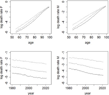
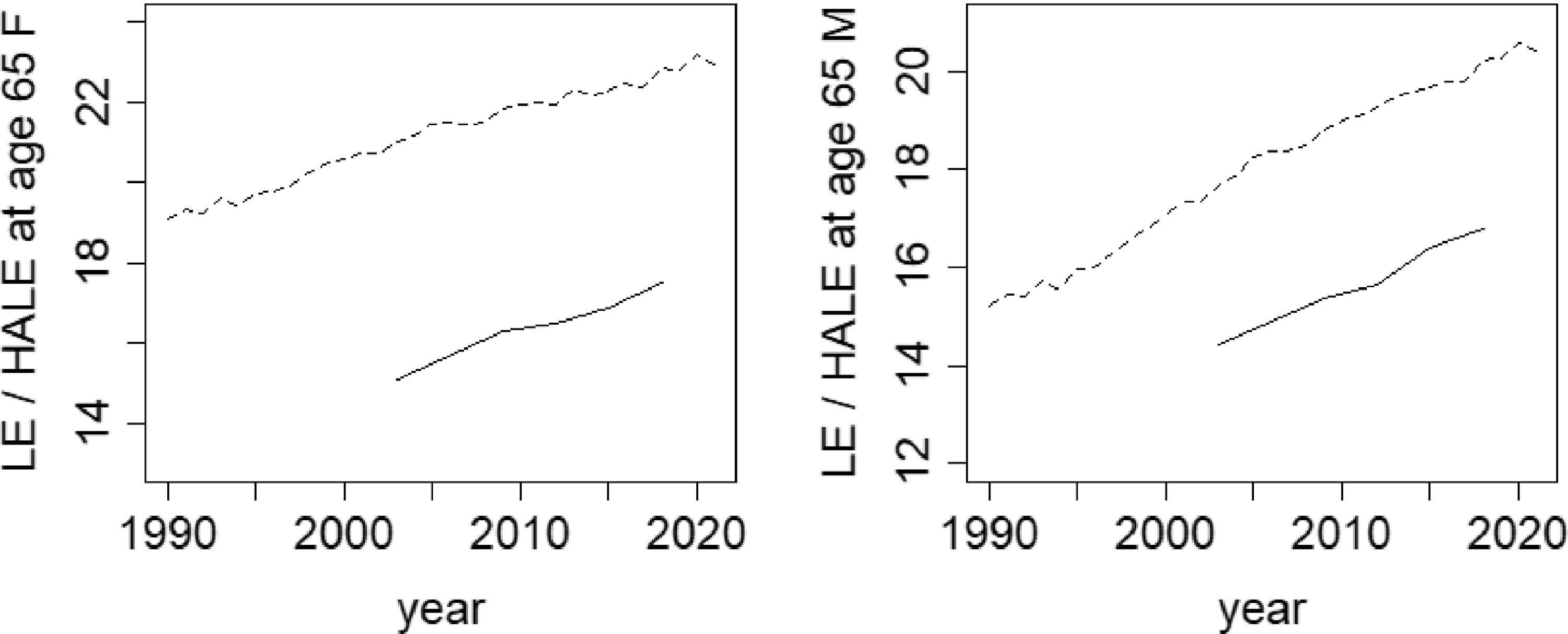
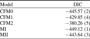
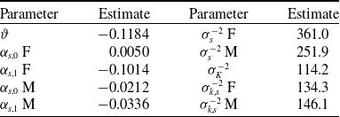

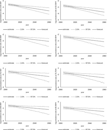
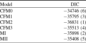
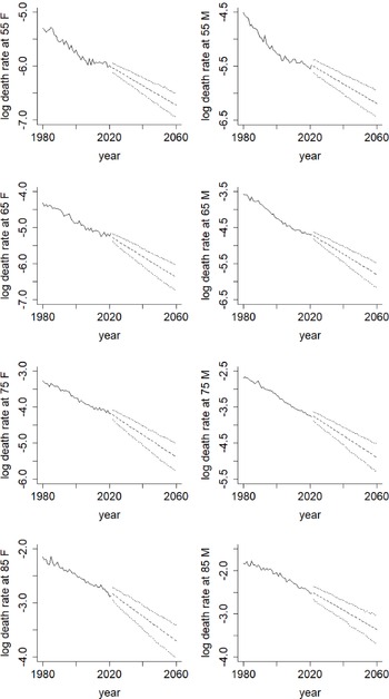
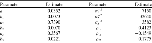
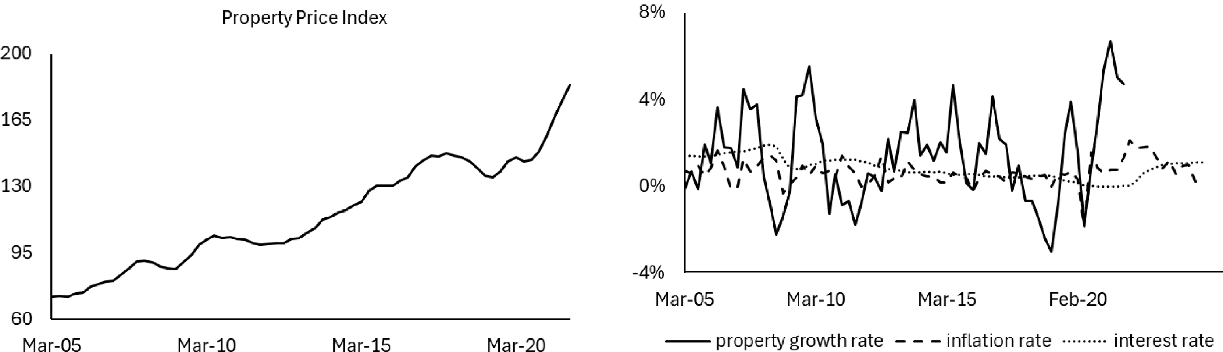
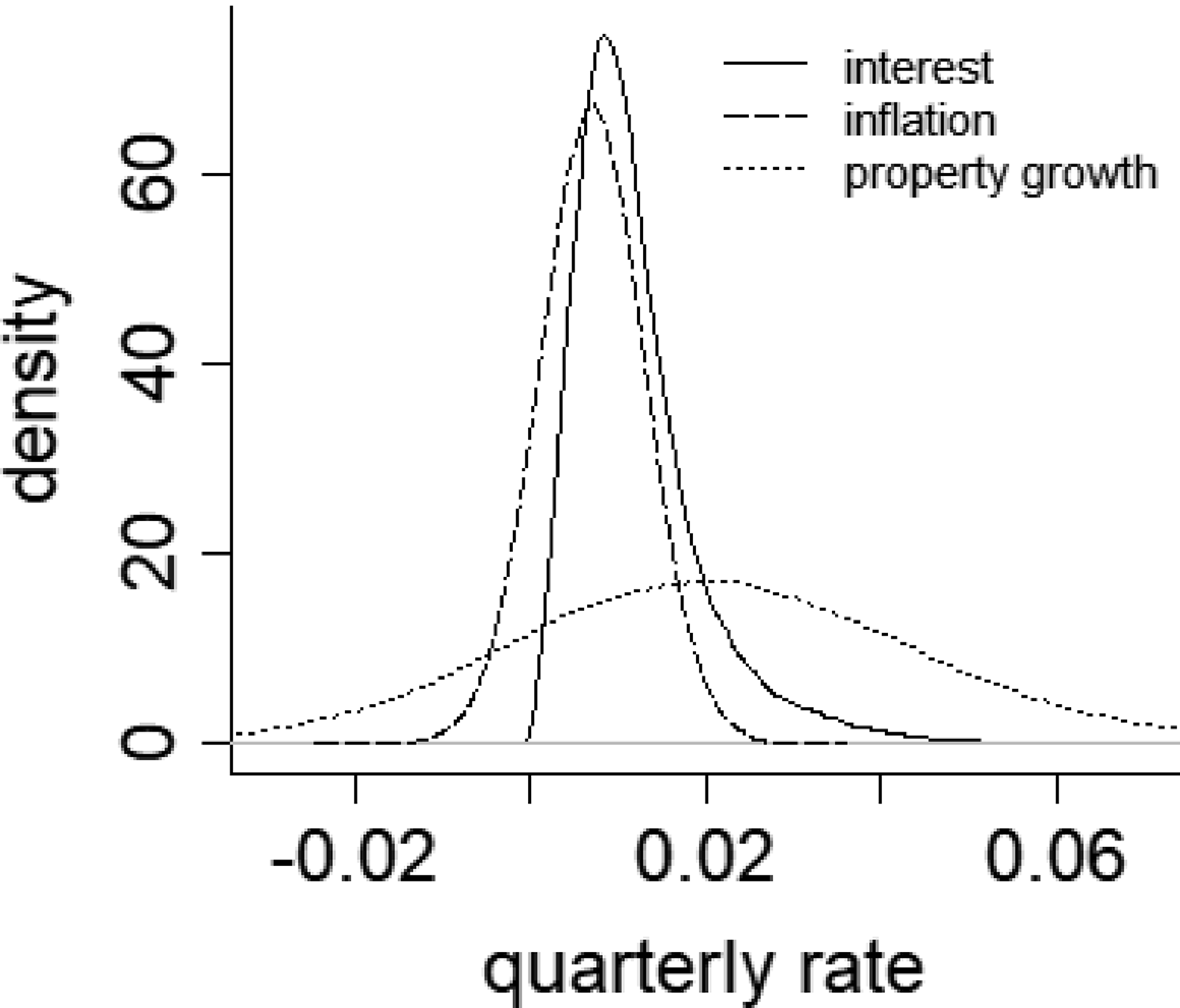


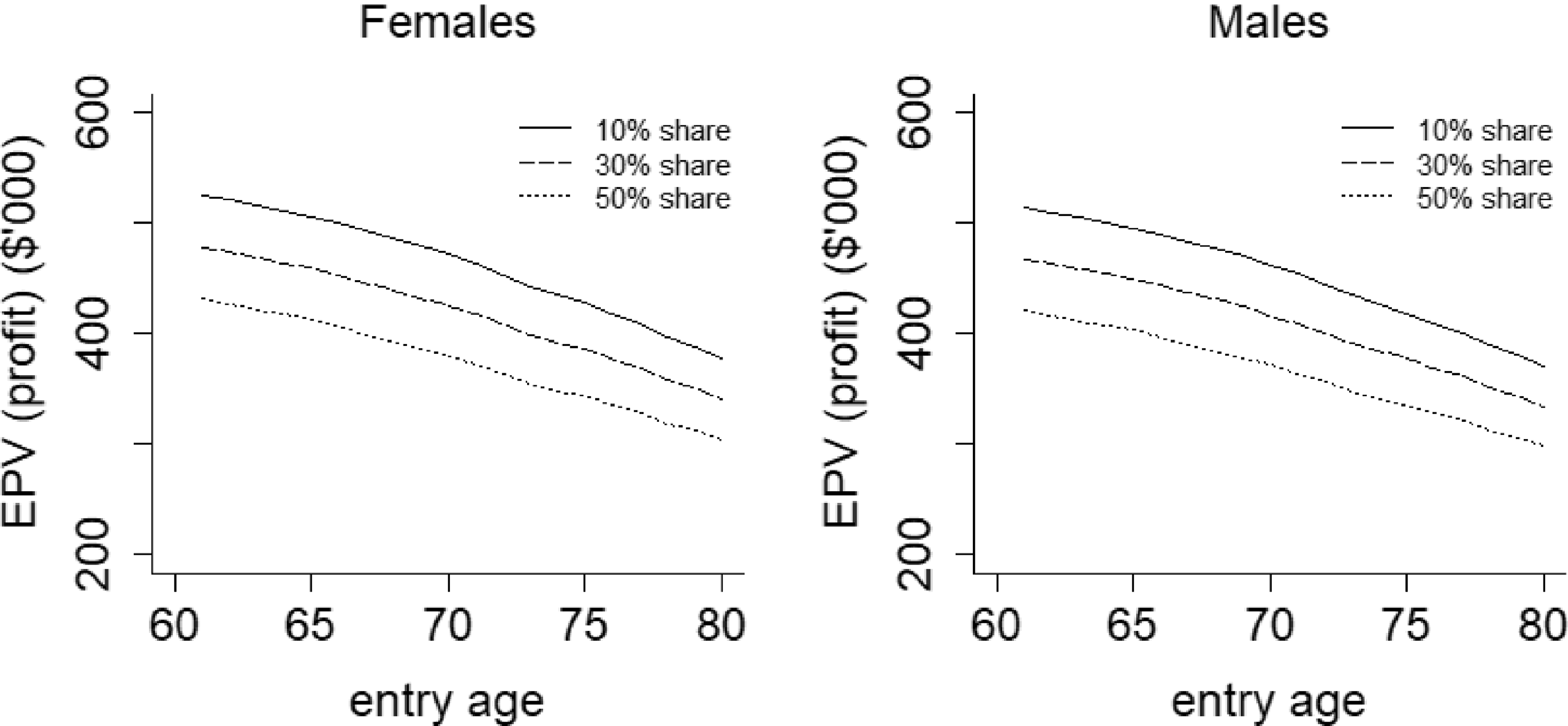

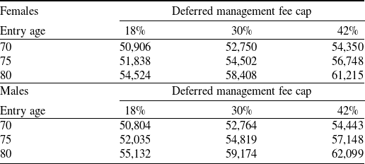

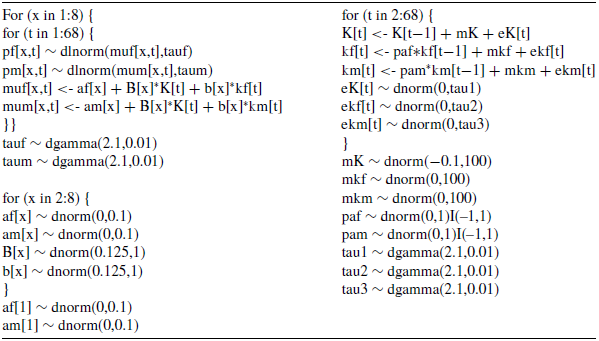
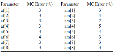

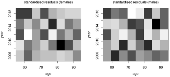
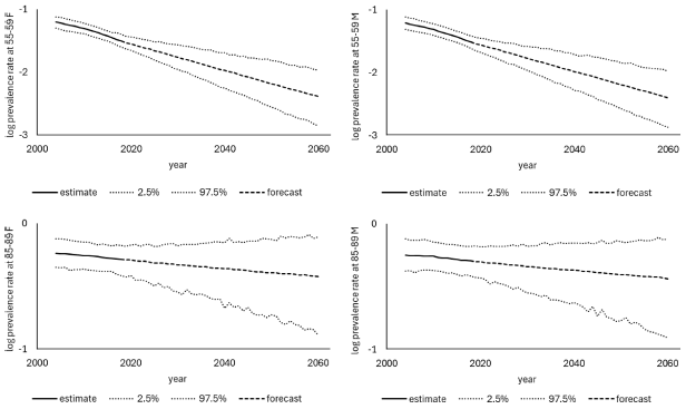
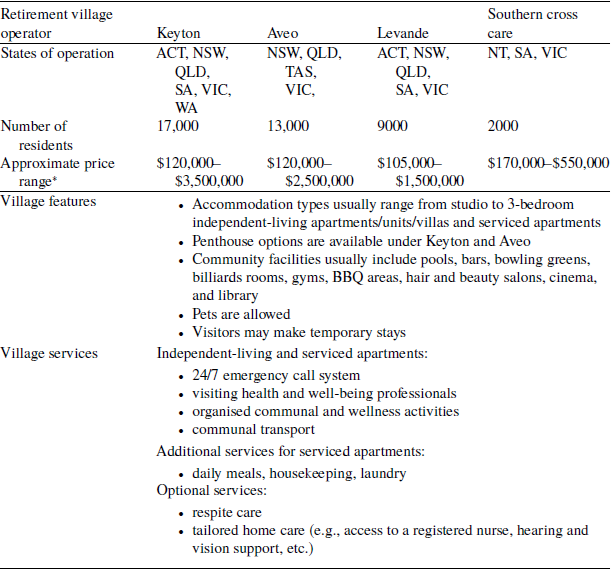

 Open access