
1. INTRODUCTION
Equation of state (EOS) describes fundamental thermophysical properties of matter. This information can only be obtained by using sophisticated theoretical models or from experiments (Al'tshuler, Reference Al'tshuler1965; Bushman & Fortov, Reference Bushman and Fortov1983; Eliezer et al., Reference Eliezer, Ghatak and Hora1986; Ross, Reference Ross1985; Chisolm et al., Reference Chisolm, Crockett and Wallace2003). The EOS is of considerable interest for basic research and has numerous important applications (Bushman et al., Reference Bushman, Lomonosov and Fortov1992, Reference Bushman, Kanel, Ni and Fortov1993; Fortov & Yakubov, Reference Fortov and Yakubov1999; Hoffmann et al., Reference Hoffmann, Fortov, Lomonosov, Mintsev, Tahir, Varentsov and Wieser2002, Reference Hoffmann, Blazevic, Ni, Rosmej, Roth, Tahir, Tauschwitz, Udrea, Varentsov, Weyrich and Maronn2005; Tahir et al., Reference Tahir, Deutsch, Fortov, Gryaznov, Hoffmann, Kulish, Lomonosov, Mintsev, Ni, Nikolaev, Piriz, Shilkin, Spiller, Shutov, Temporal, Ternovoi, Udrea and Varentsov2005b, Reference Tahir, Kim, Lomonosov, Grigoriev, Piriz, Weick, Geissel and Hoffmann2007; Temporal et al., Reference Temporal, Cela, Lopez, Piriz, Grandjouan, Tahir and Hoffmann2005), among them also inertial confinement fusion (Peng et al., Reference Peng, Zhang, Zhang, Tang, Zheng, Zheng, Wei, Ding, Gou, Zhou and Pei2005; Danson et al., Reference Danson, Brummitt, Clarke, Collier, Fell, Frackiewicz, Hawkes, Hernandez-Gomez, Holligan, Hutchinson, Kidd, Lester, Musgrave, Neville, Neely, Norreys, Pepler, Reason, Shaikh, Winstone, Wyatt and Wyborn2005; Eliezer et al., Reference Eliezer, Murakami and Val2007). High intensity heavy ion beams as well as high power lasers and pulsed power discharges are developing into an important tool for EOS experiments (Danson et al., Reference Danson, Brummitt, Clarke, Collier, Fell, Frackiewicz, Hawkes, Hernandez-Gomez, Holligan, Hutchinson, Kidd, Lester, Musgrave, Neville, Neely, Norreys, Pepler, Reason, Shaikh, Winstone, Wyatt and Wyborn2005; Jungwirth, Reference Jungwirth2005; Hoffmann et al., Reference Hoffmann, Blazevic, Ni, Rosmej, Roth, Tahir, Tauschwitz, Udrea, Varentsov, Weyrich and Maronn2005; Ray et al., Reference Ray, Srivastava, Kondayya and Menon2006; Sasaki et al., Reference Sasaki, Yano, Nakajima, Kawamura and Horioka2006; Desai et al., Reference Desai, Dezulian and Batani2007). States of matter characterized by high-energy-density occupy a broad region of the phase diagram, for example, hot compressed matter, strongly coupled plasmas, hot expanded liquid and quasi-ideal plasmas. Our knowledge of these states is limited, because theoretical modeling is complicated and experiments are difficult to perform.
Aluminum remains one of the most important metals for mankind, being of wide use in industry and science. Its thermodynamic properties have been investigated in numerous static and dynamic experiments and explored with the use of modern theories as well.
Nevertheless, the EOS for aluminum is still a “hot” problem in the physics of high energy densities. This fact is explained by a long–time intrigue of the structural phase transition at ≃ 200 GPa, inferred from the non-monotonic behavior of the shock adiabat. Other reasons are that properties of liquid aluminum at high pressures and temperatures are not well-known and multi-phase EOSs for aluminum have been developed in 1980 (Holian, Reference Holian1986; Kerley, Reference Kerley1987; Bushman et al., Reference Bushman, Kanel, Ni and Fortov1993).
Fortunately, recent progress achieved in both experimental and theoretical areas, i.e., Z-machine, diamond anvils, and quantum molecular dynamic calculations, significantly clarified these old problems. These advances motivated the present reassessment and refinement of the multi-phase EOS for aluminum.
It this work, an advanced multi-phase EOS for aluminum is presented. The thermodynamically complete, temperature EOS for metals is defined by the potential of free energy describing the elastic contribution at T = 0 K and the thermal contribution by atoms and electrons. The EOS provides for a correct description of phase boundaries, melting, and evaporation, as well as the effects of the first and second ionization. The atomic thermal contribution in the model is different in the solid and liquid states, while the electron thermal contribution is identical.
To construct the EOS, the following information was used at high pressure and high temperature: measurements of isothermal compressibility in diamond anvil cells, isentropic–compression experiments, data on sound velocity and liquid metal density at atmospheric pressure, isobaric–expansion measurements, data on the shock compressibility of solid and porous samples in incident and reflected shock waves, impedance measurements of shock compressibility obtained by an underground nuclear explosion, data on the isentropic expansion of shocked metals, calculations by the Thomas–Fermi model and by quantum molecular dynamics methods, numerous evaluations of the critical point.
New experimental and theoretical data helped to improve the description of the high-pressure, high-temperature aluminum liquid. The present EOS describes with high accuracy and reliability the complete set of available information.
2. EOS PROBLEM
EOS is a fundamental property of matter defining its thermodynamic characteristics in a functional form like f(x, y, z) = 0, where x, y, z can be, for example, volume V, pressure P, temperature T, or in the form of graphs or tables. Well-known functional for EOSs include, for instance, the Mie–Grüneisen EOS Grüneisen (Reference Grüneisen1912)
where the index c indicates the component at T = 0 K; the Birch (Reference Birch1968) potential
in which σ = V 0/V, V 0—specific volume at normal conditions (P = 1 bar, T = 298 K), B T = −(∂ P/∂ ln V)T—isothermal bulk compression modulus, B P = ∂B T/∂P—its pressure derivative; and the Carnahan–Starling's approximation for the free energy of a system of “hard” spheres (Carnahan & Starling, Reference Carnahan and Starling1969)
where N–amount of particles, k–Boltzmann's constant, and η–packing density. One can find examples of EOSs in graphic or tabular form in compendia of shock wave data (van Thiel, Reference van Thiel1977; Marsh, Reference Marsh1980; Zhernokletov et al., Reference Zhernokletov, Zubarev, Trunin and Fortov1996; Trunin et al., Reference Trunin, Gudarenko, Zhernokletov and Simakov2001); these are EOSs of shock adiabats.
The current state of the problem of a theoretical description of thermodynamic properties of matter at high pressures and high temperatures is given in a set of publications (Zeldovich & Raizer, Reference Zeldovich and Raizer1966; Eliezer et al., Reference Eliezer, Ghatak and Hora1986; Fortov & Yakubov, Reference Fortov and Yakubov1999; Bushman et al., Reference Bushman, Kanel, Ni and Fortov1993; Bushman & Fortov, Reference Bushman and Fortov1983; Ross, Reference Ross1985, and references therein). In spite of the significant progress achieved in predicting EOS information accurately in solid, liquid, and plasma states with the use of the most sophisticated “ab initio” computational approaches (classic and quantum methods of self-consisted field, diagram technique, Monte-Carlo, and molecular dynamics methods), the disadvantage of these theories is their regional character (Eliezer et al., Reference Eliezer, Ghatak and Hora1986; Fortov & Yakubov, Reference Fortov and Yakubov1999; Bushman et al., Reference Bushman, Kanel, Ni and Fortov1993; Bushman & Fortov, Reference Bushman and Fortov1983; Ross, Reference Ross1985). The range of applicability of each method is local and, rigorously speaking, no single one of them provides for a correct theoretical calculation of thermodynamic properties of matter on the whole phase plane from the cold crystal to the liquid and hot plasmas (Bushman & Fortov, Reference Bushman and Fortov1983; Eliezer et al., Reference Eliezer, Ghatak and Hora1986; Fortov & Yakubov, Reference Fortov and Yakubov1999). The principal problem here is the need to account correctly for the strong collective interparticle interaction in disordered media, which presents special difficulties in the region occupied by dense, disordered, nonideal plasmas (Bushman & Fortov, Reference Bushman and Fortov1983; Ross, Reference Ross1985; Eliezer et al., Reference Eliezer, Ghatak and Hora1986; Fortov & Yakubov, Reference Fortov and Yakubov1999; Bushman et al., Reference Bushman, Kanel, Ni and Fortov1993).
In this case, experimental data at high pressures and high temperatures are of particular significance, because they serve as reference points for theories and semi-empirical models. Data obtained with the use of dynamic methods (see Zeldovich & Raizer, Reference Zeldovich and Raizer1966; Bushman et al., Reference Bushman, Kanel, Ni and Fortov1993; Fortov & Yakubov, Reference Fortov and Yakubov1999; McQueen et al., Reference McQueen, Marsh, Taylor, Fritz, Carter and Kinslow1970; Avrorin et al., Reference Avrorin, Vodolaga, Simonenko and Fortov1990; Al'tshuler Reference Al'tshuler1965; Duvall & Graham, Reference Duvall and Graham1977, and references therein) are of the importance from the practical point of view. Shock-wave methods permit to study a broad range of the phase diagram from the compressed hot condensed states to dense strongly coupled plasma and quasi-gas states. Detailed presentations of shock-wave methods to investigate high dynamic pressures can be found in the literature (Zeldovich & Raizer, Reference Zeldovich and Raizer1966; Bushman et al., Reference Bushman, Kanel, Ni and Fortov1993; Fortov & Yakubov, Reference Fortov and Yakubov1999; Avrorin et al., Reference Avrorin, Vodolaga, Simonenko and Fortov1990, and reviews, Al'tshuler, Reference Al'tshuler1965; Duvall & Graham, Reference Duvall and Graham1977).
Available experimental data on the shock compression of solid and porous metals, as well as isentropic expansion, covers nine orders of magnitude in pressure and four in density. The first published shock-wave data were obtained for metals in the megabar (1 Mbar = 100 GPa) (Walsh et al., Reference Wang, Chen and Zhang1957) and multimegabar (Al'tshuler et al., Reference Al'tshuler, Krupnikov, Ledenev, Zhuchikhin and Brazhnik1958a, Reference Al'tshuler, Krupnikov, Ledenev, Zhuchikhin and Brazhnik1958b) pressure range using explosive drivers. Higher pressures of 10 Mbar have been accessed by spherical cumulative systems (Kormer et al., Reference Kormer, Funtikov, Urlin and Kolesnikova1962; Al'tshuler et al., Reference Al'tshuler, Bakanova, Dudoladov, Dynin, Trunin and Chekin1981) and by underground nuclear explosions (Al'tshuler et al., Reference Al'tshuler, Moiseev, Popov, Simakov and Trunin1968; Trunin et al., Reference Trunin, Podurets, Moiseev, Simakov and Popov1969). Maximum pressures of 400 TPa (Vladimirov et al., Reference Volkov, Voloshin, Vladimirov, Nogin and Simonenko1984) were also reported for aluminum through the use of nuclear explosion. Note that data obtained by impedance-matching techniques require the knowledge of the EOS for a standard material. Previously a monotonic approximation of the shock adiabat of lead between the traditional region of pressures ≤10 Mbar to Thomas–Fermi calculations (Kalitkin & Kuzmina, Reference Kalitkin and Kuzmina1975) was used for the standard (Al'tshuler et al., Reference Al'tshuler, Moiseev, Popov, Simakov and Trunin1968; Trunin et al., Reference Trunin, Podurets, Moiseev, Simakov and Popov1969). It seems that iron, for which absolute Hugoniot measurements have been reported to pressures of 100 Mbar (Trunin et al., Reference Trunin, Podurets, Popov, Zubarev, Bakanova, Ktitorov, Sevastyanov, Simakov and Dudoladov1992, Reference Trunin, Podurets, Moiseev, Simakov and Sevastyanov1993), is now the best etalon material. Figure 1 shows modern progress achieved in measurements of absolute shock compressibility with the use of traditional explosive techniques and investigations of impedance in experiments with concentrated energy fluxes like lasers and underground nuclear explosions.
The investigated pressure scale for the elements. Shown are maximum pressures achieved using traditional explosive (gray region), lasers, diamond-anvil-cell static measurements (black), and underground nuclear explosions (points).

The extension of the phase diagram data to greater relative volumes, in comparison with the principal Hugoniot, is achieved with shock compression of porous samples (Zeldovich & Raizer, Reference Zeldovich and Raizer1966). Nevertheless, difficulties in fabricating highly porous targets and non-uniform material response of the porous sample to shock loading imposes a practical limit to the minimum density of a specimen. The method of isentropic expansion of shocked matter, depending on the magnitude of the shock pressure and, consequently, the entropy provided, produces in one experiment transitions from a hot metallic liquid shocked state, to a strongly coupled plasma, then to a two-phase liquid-gas region, and to a Boltzmann's weakly ionized plasma, and finally to a nearly ideal gas (Zeldovich & Raizer, Reference Zeldovich and Raizer1966; Bushman et al., Reference Bushman, Kanel, Ni and Fortov1993; Fortov & Yakubov, Reference Fortov and Yakubov1999).
The available experimental and theoretical information is shown in Figure 2 on a three-dimensional (3D), relative volume-temperature-pressure surface calculated by a semi-empirical multi-phase EOS (Bushman et al., Reference Bushman, Kanel, Ni and Fortov1993). It is well illustrated that besides the shock compressibility, measurements of release isentropes of shocked materials are of especial importance. Such results traverse states in the intermediate region between the solid state and gas, occupied by a hot dense metallic liquid and strongly coupled plasma (Bushman et al., Reference Bushman, Kanel, Ni and Fortov1993; Fortov & Yakubov, Reference Fortov and Yakubov1999), which is a region poorly described by theory. Experimentally studied release isentropes for copper have as initial high energy states solid, and melted, and compressed liquid metal. The range of thermodynamic parameters covered in the adiabatic expansion process for these states is extremely wide (Fig. 2), covering five orders of magnitude in pressure and two orders of magnitude in density. It extends from a highly compressed metallic liquid, characterized by a disordered arrangement of ions, and degenerate electrons, to a quasi-nonideal Boltzmann plasma and a rarefied metallic vapor. Upon expansion of the system, the degree of degeneracy of the electronic subsystem is decreased and a marked rearrangement of the energy spectrum of atoms and ions occurs. A partial recombination of the dense plasma also takes place. In the disordered electron system, a “metal-insulator” transition takes place and a nonideal (with respect to different forms of interparticle interactions) plasma is formed in the vicinity of the liquid-vapor equilibrium curve and the critical point. Where the isentropes enter the two-phase liquid-vapor region evaporation occurs; on the gas-side condensation occurs (Avrorin et al., Reference Avrorin, Vodolaga, Simonenko and Fortov1990; Bushman et al., Reference Bushman, Kanel, Ni and Fortov1993; Fortov & Yakubov, Reference Fortov and Yakubov1999).
Generalized 3D volume-temperature-pressure surface for copper in the investigated region of the phase diagram. M–melting region; H 1 and H p–principal and porous Hugoniots; DAC–diamond-anvil-cells data; IEX–isobaric expansion data; S–release isentropes; R–boundary of two-phase liquid-gas region with the critical point CP. Phase states of the metal are also shown.

Note that typical shock-wave measurements allow determination of only caloric properties of matter, viz. the dependence of the relative internal energy on pressure and volume as E = E(P, V). The potential E(P, V) is not complete in the thermodynamic sense and a knowledge of temperature T or entropy S is required for completing the thermodynamic equations and calculating first and second derivatives, such as the heat capacity, the sound velocity and others (Fortov & Yakubov, Reference Fortov and Yakubov1999).
Only a few temperature measurements in shocked metals are available (Yoo et al., Reference Yoo, Holmes, Ross, Webb and Pike1993), as well as analogous measurements in release isentropic waves (Avrorin et al., Reference Avrorin, Vodolaga, Simonenko and Fortov1990). This information is of great importance in view of a limitation of purely theoretical calculation methods. From this point of view, thermodynamically complete measurements obtained with the use of the isobaric expansion (IEX) technique (Gathers, Reference Gathers1986) are of a special significance. In this method, metal is rapidly heated by a powerful pulsed current, then expands into an atmosphere of an inertial gas maintained at constant pressure. This data range in density form solid to the critical point and intersect, therefore, the release isentrope data for metals (see Fig. 2).
The region between principal shock adiabat and isotherm can be accessed with use of the isentropic compression technique. This method allows one to obtain simultaneously high pressure and high densities in the material under study. In practice, the sample is loaded by a magnetically driven impactor or by a sequence of reverberating shock waves in a multi-step compression process.
The final conclusion is that shock-wave techniques allow one to investigate material properties in very wide region of the phase diagram—from compressed solid to hot dense liquid, plasma, liquid-vapor, and quasi-gas states. Though the resulting high pressure, high and temperature information covers a broad range of the phase diagram, it has a heterogeneous character and, as a rule, is not complete from the thermodynamic point of view. Its generalization can be done only in the form of a thermodynamically complete EOS.
3. EOS MODEL
Wide-range EOS models for aluminum have been developed since the 1960s (see, for example, Kormer et al., 1962; Holian, Reference Holian1986; Kerley, Reference Kerley1987; Bushman et al., Reference Bushman, Lomonosov and Fortov1992, Reference Bushman, Kanel, Ni and Fortov1993; Young & Corey, Reference Young and Corey1995). The model described below presents a modification of an existing EOS of Bushman et al. (Reference Bushman, Kanel, Ni and Fortov1993). Changes are in the thermal electrons and the cold compression curve, which are from Bushman et al. (Reference Bushman, Lomonosov and Fortov1992).
The EOS model is given by a thermodynamically complete potential of free energy F in the traditional form
describing the elastic contribution at T = 0 K (F c), and the heat contribution by atoms (F a) and electrons (F e).
3.1. Elastic Curve
The elastic energy for the solid phase is given in the form of a series expansion of r c−1 ~ σc1/3 (Kormer et al., Reference Kormer, Funtikov, Urlin and Kolesnikova1962; Bushman et al., Reference Bushman, Lomonosov and Fortov1992, Reference Bushman, Kanel, Ni and Fortov1993)
where σc = V 0c/V, V 0c–specific volume at P = 0. Note that Eq. (5) automatically provides for the normalizing condition F c(s)(V 0c) = 0.
The conditions at σc = 1 for the cold pressure P c(V) = −dF c(V)/dV, bulk compression modulus B c(V) = −VdP c(V)/dV, and its pressure derivative B p(V) = dB c/dP c define the cold curve at moderate compressions, which together with Eq. (5) leads to the formulas


Here B 0c and B p0, together with the thermal contribution, provide for tabular values of the isentropic bulk compression modulus and its pressure derivative at normal conditions. By minimizing the mean-square deviation from the Thomas-Fermi cold pressure P cTFC (Kalitkin & Kuzmina, Reference Kalitkin and Kuzmina1975) over N points in the interval of σc from 25 to 500, together with the bounding equations (6)–(8), one can define the Lagrangian problem of determining the minimum of the functional form depending on χ = a i, λ, μ, ν
![\eqalign{\Upsilon\lpar \chi\rpar& = \sum_{n=1\comma N}g_{n} \left[1- {P_{c}\lpar a_{i}\comma\; \sigma_{n}\rpar \over P_{c}^{TFC}\lpar \sigma_{n}\rpar }\right]^{2}\cr&\quad + \lambda \sum_{i=1\comma 5}a_{i}+ \mu \left(B_{0c}-\sum_{i=1\comma 5}a_{i} {i \over 3}\right)\cr &\quad+ \nu \left(B_{\,p0}-2- {1\over B_{0c}}\sum_{i=1\comma 5}a_{i}\left({i \over 3}\right)^{2}\right).}](https://static.cambridge.org/binary/version/id/urn:cambridge.org:id:binary:20151021081604112-0734:S0263034607000687_eqn9.gif?pub-status=live)
Taking derivatives of Eq. (9) on a i, λ, μ, ν one can obtain the algebraic system of eight linear equations for eight values, whose solution defines the coefficients a i.
The cold energy for the liquid in the compression region (σc ≥ 1) is given by Eq. (5), while in the rarefaction region (σc < 1) it is represented as
The normalizing condition F c(l)(σc = 0) = E sub, where E sub is the tabular value of the cohesion energy, leads to the formula
The system of Eqs. (6)–(8) for a cold energy in the form of Eq. (10) at σc=1 results in
Here parameter m is usually ≈ 1 (i.e., van der Waals); l is a fitting parameter, defined from the best description of the density and sound velocity data in the liquid phase. Other parameters are found from Eqs. (11)–(14).
3.2. Thermal Contribution of Atoms
The atomic thermal contribution to the free energy of the solid phase is defined by the high-temperature Debye approximation formula:
where R is the gas constant. The characteristic temperature θc(s) is given by the empirical relation
![\eqalign{\theta_{c}^{\lpar s\rpar }\lpar V\rpar =\theta_{0}^s \sigma ^{2/3} \exp \left({\lpar \gamma_{0s}-2/3\rpar \lpar B_{s}^{2} + D_{s}^{2}\rpar \over B_{s}}\right. \cr \quad \left. \arctan \left[{xB_{s} \over B_{s}^{2} + D_{s}\lpar x + D_{s}\rpar }\right]\right)\comma}](https://static.cambridge.org/binary/version/id/urn:cambridge.org:id:binary:20151021081604112-0734:S0263034607000687_eqn16.gif?pub-status=live)
where x = lnσ. Constants B s and D s are found from the compression dependence of the Grüneisen gamma γ(V) = dlnθ(V)/dlnσ. This information is obtained from shock-wave and isentropic–compression data in the solid state. The value of γ0s is the tabulated value of the Grüneisen parameter at ambient conditions, and the normalizing condition for entropy S(V 0, T = 293 K) = 0 defines the value of θ0s. Note that at high compression Eq. (16) provides for the correct ideal-gas asymptote θc(s) ~ σ2/3.
The atomic thermal contribution to the free energy of the liquid phase is represented as
The first term accounts for anharmonic effects and the second provides for a properly behaved melting curve.
In the liquid phase, the phonon contribution has a form similar to Eq. (16) but with a volume- and temperature-dependent heat capacity c a and a characteristic temperature θ(l):
The heat capacity in the liquid phase is given by the expression
describing a smooth variation from the value 3R close to the lattice heat capacity to that of an ideal atomic gas, 3R/2. Coefficients σa and T a define the characteristic density and temperature of this transition.
The variation of the characteristic temperature defines the vibrational spectrum and reflects the gradual change of the Grüneisen coefficient of the liquid phase from values γ(l) ≈ γ(s), corresponding to condensed states, to the ideal-gas value of 2/3 in the limit of high temperatures and very low densities. Under these assumptions, the characteristic temperature is given by the approximating formula
where the characteristic temperature in the liquid phase is given in a form analogous to Eq. (16)
![\eqalign{\theta_{c}^{\lpar l\rpar }\lpar V\rpar =\theta_{0}^l \exp \left({\lpar \gamma_{0l}-2/3\rpar \lpar B_{l}^{2} + D_{l}^{2}\rpar \over B_{l}}\right. \cr \quad \left. \times \arctan \left[{xB_{l} \over B_{l}^{2} + D_{l}\lpar x + D_{l}\rpar }\right]\right).}](https://static.cambridge.org/binary/version/id/urn:cambridge.org:id:binary:20151021081604112-0734:S0263034607000687_eqn21.gif?pub-status=live)
The parameters in Eq. (21), B l and D l, are found from shock-wave experiments for solid and porous samples, while the constant θ0l is determined by equation θc(l)(0) = T ca.
The potential term F m(V, T) provides for correct values of the entropy changes ΔS = ΔS m0 and volume changes ΔV = ΔV m0 on melting at ambient pressure, and disappears in the gas phase. The contribution of F m should also decrease upon compression due to decreasing differences between the properties of the solid and liquid phases. These requirements are satisfied by the relation
![\eqalign{F_{m}\lpar V\comma\; T\rpar &=3R \left({2\sigma_{m}^{2} T_{m0} \over 1 + \sigma_{m}^3} \left[C_{m} + {3A_{m} \over 5}\lpar \sigma_{m}^{5/3}-1\rpar \right]\right. \cr &\quad \left. + \lpar B_{m}-C_{m}\rpar T \right)\comma}](https://static.cambridge.org/binary/version/id/urn:cambridge.org:id:binary:20151021081604112-0734:S0263034607000687_eqn22.gif?pub-status=live)
where σm = σ/σm0 is the relative density of the liquid phase on the melting curve. The constants A m, B m, and C m are uniquely determined by the equilibrium conditions along the melting curve at T = T m.
3.3. Thermal Contribution of Electrons
The electronic thermal contribution has an identical form for the solid and liquid phases. It is given by
It includes the generalized analog of the coefficient of the electronic heat capacity B e:
the coefficient of the electronic heat capacity β:
the heat capacity of the electron gas c ei
and the analog of the electronic Grüneisen coefficient γe:

Approximating dependencies are written in this manner to satisfy primarily the asymptotic relations for the electron gas free energy, namely expressions for the degenerate electron gas F e(V, T) =−β0T 2σ−γ0/2 at moderate temperatures (T ≪ T Fermi) and expressions for an ideal electron gas F e(V, T) = 3RZ ln(σ2/3T)/2 as T → ∞. Here Z is the atomic number and R is the gas constant. The specific forms given for the separate terms of Eq. (23) were chosen to satisfy these requirements.
Eqs. (23)–(28) are written in a form which correctly represents the primary ionization effects in the plasma region and the behavior of the partially ionized metal. Eq. (27) for τi describes a decrease of the ionization potential as the plasma density increases, and the constants σz and T z define, respectively, the characteristic density of the “metal-insulator” transition and the temperature dependence of the transition from a singly ionized gas to a plasma with the ion–charge mean value Z.
3.4. EOS Construction Procedure
The set of Eqs. (4)–(28) fully defines the thermodynamic potential for metals over the entire phase diagram for the region of practical interest. Some coefficients in the EOS, included in the analytical expressions, are constants characteristic for each metal (atomic weight and charge, density at normal conditions and other) and are obtained from tabulated data. The rest serve as fitting parameters and their values are found from the optimum description of the available experimental and theoretical data, while providing for correct asymptotes to calculations based on the Debye–Hückel and Thomas–Fermi theories (Kalitkin & Kuzmina, Reference Kalitkin and Kuzmina1975). It should be emphasized that, even though the number of coefficients in Eqs. (4)–(28) is large, most of them are rigidly defined constants whose values are assigned explicitly or implicitly from the fulfillment of various thermodynamic conditions at specific points on the phase diagram. A few coefficients (about 10) serve to characterize the densities and temperatures of transition from one typical phase-plane region to another and are found empirically. The tables in the appendix lists the parameters of the EOS model given by Eqs. (4)–(28) along with the values for aluminum.
The numerous experimental and theoretical data characterizing the thermodynamic properties of metals for a wide range of parameters, was used in determining the numerical values of coefficients in the EOS, This procedure was carried out with the aid of a specially developed computer program using Eqs. (4)–(28) for thermodynamic calculations. At the preliminary stage of calculations, some thermodynamic constants known for each substance (such as normal density, changes in density and entropy at the melting point under normal pressure, cohesion energy, and the like) were used by the program automatically for finding a number of other uniquely defined coefficients (parameters of the cold curve, melting curve, and so on). This further enables one, by way of calculating algebraic or integral relations valid for self-similar hydrodynamic flows, to perform calculations of the kinematic characteristics measured experimentally at high and ultrahigh pressures, namely, the incident and reflected wave velocities and velocities in adiabatic expansion waves (release isentropes), as well as to allow for melting and evaporation effects. The range of action of each fitting parameter that remains free is very localized, as a result of which its value may be selected independently from a comparison of the calculations with available experimental data.
The EOS was constructed using the following high pressure, high temperature information: measurements of isothermal compressibility in diamond anvil cells, data on sound velocity and density in liquid metals at atmospheric pressure, IEX measurements, data on the shock compressibility of solid and porous samples in incident and reflected shock waves, impedance measurements of shock compressibility using an underground nuclear explosion, data on isentropic expansion of shocked metals, calculations by quantum molecular dynamics (QMD), Debye–Hückel, and Thomas–Fermi models, and evaluations of the critical point.
All of the experimental and theoretical data have a given history of accuracy and reliability. The major problem in EOS construction is to provide for a self-consistent and non-contradictory description of the many kinds of available data.
4. THERMODYNAMIC PROPERTIES OF ALUMINUM
This section presents the calculation results of the thermodynamic properties and the phase diagram of aluminum. This is done with the use of Eqs. (4)–(28). The resulting dependencies are compared with the experimental data and theoretical calculations that are most significant at high pressures and temperatures.
All data are presenting in graphs. Earlier results of Al'tshuler et al. (Reference Al'tshuler, Krupnikov and Brazhnik1958a, Reference Al'tshuler, Krupnikov, Ledenev, Zhuchikhin and Brazhnik1958b, Reference Al'tshuler, Kormer, Bakanova and Trunin1960a; McQueen et al., Reference McQueen, Marsh, Taylor, Fritz, Carter and Kinslow1970; van Thiel, Reference van Thiel1977) have been revised several times. The effects of impactor heating and an attenuation of the shock in the window and specimen have been analyzed (Al'tshuler & Chekin, Reference Al'tshuler and Chekin1984), and the corrections have been applied based on new precise shock adiabats of reference materials (Marsh, Reference Marsh1980; Zhernokletov et al., Reference Zhernokletov, Zubarev, Trunin and Fortov1996; Trunin et al., Reference Trunin, Gudarenko, Zhernokletov and Simakov2001). The experimental shock wave data in the graphs correspond to the most recent reported values, for which accounting have been made for all of these experimental factors.
The present EOS accounts for the theoretical and experimental data published up to the middle of 2007. The parameters of the liquid state have been changed strongly, in comparison with the predecessor aluminum EOS of Busman et al. (Reference Bushman, Kanel, Ni and Fortov1993), to satisfy new high pressure Hugoniot data, isothermal (Akahama et al., Reference Akahama, Nishimura, Kinoshita and Kawamura2006) and isentropic compression measurements (Davis, Reference Davis2006) and the results of quantum molecular dynamic calculations (Desjarlais, personal communication) in the critical point region.
4.1. Crystal
Aluminum has an face-centered cubic (fcc) structure at room pressure and temperature. The structural fcc hexagonal close packed (hcp) phase transition at T = 0 K has been predicted by different theories (Voropinov et al., Reference Walsh, Rice, McQueen and Yarger1970; McMahan & Moriarty, Reference McMahan and Moriarty1983; Lam & Cohen, Reference Lam and Cohen1983; Wentzcovich & Law, 1991; Boettger & Trickey, Reference Boettger and Trickey1996) to occur at pressures of 120–360 GPa. According to (Greene et al., Reference Greene, Luo and Ruoff1994) it remains a simple solid to a pressure of 220 GPa under isothermal compression in a diamond anvil cell, but in analogous experiment (Akahama et al., Reference Akahama, Nishimura, Kinoshita and Kawamura2006) at 217 GPa aluminum transforms to hcp phase with a volume reduction of 1%. Novel high-pressure data on isentropic compression of aluminum (Davis, Reference Davis2006), as well as the results of the diamond anvil cell (DAC) experiment of (Greene et al., Reference Greene, Luo and Ruoff1994; Akahama et al., Reference Akahama, Nishimura, Kinoshita and Kawamura2006), which are in the solid state region, do not demonstrate dramatic changes in the thermodynamic parameters. So the present EOS provides for a monotonic compression curve.
A comparison of the cold curve, found using Eqs. (5)–(9), with the results of band–structure calculations is shown in Figure 3. It is seen that the elastic curve agrees with different variants of Thomas–Fermi theory (Kalitkin & Kuzmina, Reference Kalitkin and Kuzmina1975; Perrot, Reference Perrot1979), the augmented–plane wave (APW) (McMahan & Ross, Reference McMahan and Ross1979), the self–consistent cell model (Liberman, Reference Liberman1979), and the Hartree–Fock–Slater method (Nikiforov et al., Reference Nikiforov, Novikov and Uvarov1989), as well in all ranges of densities to 100-fold compression.
Pressure in aluminum at T = 0 K. Nomenclature: line–EOS; points–theories, 1–Thomas–Fermi model with corrections Kalitkin & Kuzmina (Reference Kalitkin and Kuzmina1975), 2–self-consistent cell model Liberman, (Reference Liberman1979), 3–APW McMahan & Ross, (Reference McMahan and Ross1979), 4–Thomas–Fermi model with gradient correction Perrot (Reference Perrot1979), 5–modified Hartree–Fock–Slater model Nikiforov et al. (Reference Nikiforov, Novikov and Uvarov1989).

The room temperature isotherm to 12 GPa (Syassen & Holzaphel, Reference Syassen and Holzaphel1978), 220 GPa (Greene et al., Reference Greene, Luo and Ruoff1994) and 333 GPa (Akahama et al., Reference Akahama, Nishimura, Kinoshita and Kawamura2006) is drawn in Figure 4, along with isentropic compression data (Davis, Reference Davis2006) obtained to 300 GPa. Figure 5 also contains theoretical isotherms calculated with the use of the pseudopotential approach (Nellis et al., Reference Nellis, Moriarty, Mitchell, Ross, Dandrea, Ashcroft, Holmes and Gathers1988) and the full-potential linearized augmented plane wave method (Wang et al., Reference Wentzcovich and Lam2000). The compression curve for this EOS, which is an isentrope, is also shown. Note that the difference between the compression isentrope and isotherms, with T = 0 and 298 K, in this range of pressures of up to 340 GPa is negligible. The overall agreement between this semi-empirical compression curve and theory and experiment is good and within the error bars of the experimental data.
Pressure in solid aluminum. Nomenclature: line–EOS; points–experiment, 1–DAC Syassen & Holzaphel (Reference Syassen and Holzaphel1978), 2–DAC Greene et al. (Reference Greene, Luo and Ruoff1994), 4–isentropic compression Davis (Reference Davis2006), 6,7–DAC fcc and hcp Akahama et al. (Reference Akahama, Nishimura, Kinoshita and Kawamura2006), and theory, 3–Nellis et al. (Reference Nellis, Moriarty, Mitchell, Ross, Dandrea, Ashcroft, Holmes and Gathers1988), 5–Wang et al. (Reference Wentzcovich and Lam2000).

Aluminum melting at 1 bar and at 0.3 GPa. Nomenclature: line–EOS; points–experiment, 1–at 1 bar Hultrgen et al. (Reference Hultrgen, Desai, Hawkins, Gleiser, Kelley and Wagman1973), 2–at 0.3 GPa Gathers (Reference Gathers1983).

4.2. Melting
At room pressure, aluminum melts at T = 933 K. The experimental data (Hultrgen et al., Reference Hultrgen, Desai, Hawkins, Gleiser, Kelley and Wagman1973) at 1 bar are compared with EOS calculations in Figure 5. Less dense liquid states, characterized by higher values of enthalpy, have been measured in an IEX experiment at 0.3 GPa (Gathers, Reference Gathers1983). The calculated P = 0.3 GPa isobar is also shown in this figure. Note that these EOS isobars are clearly different, while data at 0.3 GPa (Gathers, Reference Gathers1983) correspond to the linear approximation of 1 bar measurements (Hultrgen et al., Reference Hultrgen, Desai, Hawkins, Gleiser, Kelley and Wagman1973). The analysis of Figure 4 demonstrates the reliability of the developed EOS in this region of the phase diagram.
The high-pressure melting curve is plotted in the pressure-temperature diagram of Figure 6. The extrapolation of static DAC measurements (Boehler & Ross, Reference Boehler and Ross1997; Hanstrom & Lazor, Reference Hanstrom and Lazor2000) is in good agreement with the results of a dynamic experiment (McQueen et al., Reference McQueen, Fritz, Morris, Asay, Graham and Straub1984), according to which aluminum melts under shock at a pressure of 110 GPa. The calculated melting line and shock adiabat show good agreement with available data.
Aluminum melting at high pressures. Nomenclature: lines–EOS calculations, M–melting, H 1–shock adiabat; points–experiment, 1–Jayaraman et al. (Reference Jayaraman, Klement and Kennedy1963), 2–Hanstrom & Lazor (Reference Hanstrom and Lazor2000), 3–Boehler & Ross (Reference Boehler and Ross1997).

4.3. Dense Aluminum at High Pressure
In this section, let us discuss the results of shock-wave measurements. Aluminum has been extensively investigated in the past 50 years. Its principal Hugoniot has been measured with the use of traditional high-explosive drivers to pressures of 200 GPa (Al'tshuler et al., Reference Al'tshuler, Kormer, Bakanova and Trunin1960a; McQueen et al., Reference McQueen, Marsh, Taylor, Fritz, Carter and Kinslow1970; Al'tshuler et al., Reference Al'tshuler, Bakanova, Dudoladov, Dynin, Trunin and Chekin1981; Marsh, Reference Marsh1980). Light-gas guns allowed one to obtain precise data to pressures of 210 GPa (Isbell et al., Reference Isbell, Shipman and Jones1968; Mitchell & Nellis, Reference Mitchell and Nellis1981). Much higher pressures of 400 GPa were accessed with the use multi-layer cumulative explosive systems (Glushak et al., Reference Glushak, Zharkov, Zhernokletov, Ternovoi, Filimonov and Fortov1989) and pressures of 990 GPa with the use of powerful hemi-spherical cumulative drivers (Skidmore & Morris, Reference Skidmore and Morris1962; Kormer et al, Reference Kormer, Funtikov, Urlin and Kolesnikova1962; Al'tshuler & Chekin, Reference Al'tshuler and Chekin1984; Trunin, Reference Trunin1986; Trunin et al., Reference Trunin, Panov and Medvedev1995a, Reference Trunin, Panov and Medvedev1995b). High-precision data up to 480 GPa were measured in Z–pinch experiments (Knudson et al., Reference Knudson, Lemke, Hayes, Hall, Deeney and Asay2003), in which aluminum flyer plates were magnetically accelerated to high velocities.
Extreme pressures in aluminum were generated with the use of underground nuclear explosions. Maximum pressures of 400 TPa were realized (Vladimirov et al., Reference Volkov, Voloshin, Vladimirov, Nogin and Simonenko1984), along with the shock limit of compression ratio. One should specially note that at higher pressures, the contribution of radiation to the pressure and energy will be more significant than the thermal contributions. So we may conclude that the EOS limit for the aluminum shock adiabat has been achieved. Absolute measurements of aluminum shock compressibility were done at 0.9–3.2 TPa (Simonenko et al., Reference Simonenko, Voloshin, Vladimirov, Nagibin, Nogin, Popov, Sal'nikov and Shoidin1985). All other measurements are referred to as nuclear impedance measurements (NIM), which are limited in the accuracy with which a reference material is known. In these works, aluminum's compressibility was studied with respect to different standard materials: quartz to pressures of 0.27–2 TPa (Al'tshuler et al., Reference Al'tshuler, Kalitkin, Kuz'mina and Chekin1977), molybdenum at 2.2–2.9 TPa (Ragan, Reference Ragan1982, Reference Ragan1984), and iron at 4.3–28.9 TPa (Avrorin et al., Reference Avrorin, Vodolaga, Voloshin, Kuropatenko, Kovalenko, Simonenko and Chernodolyuk1986), 1.7 TPa (Podurets et al., Reference Podurets, Ktitorov, Trunin, Popov, Matveev, Pechenkin and Sevast'yanov1994), and 0.25–1.27 TPa (revision Trunin et al., Reference Vladimirov, Voloshin, Nogin, Petrovtsev and Simonenko2001) of data in Avrorin et al., Reference Avrorin, Vodolaga, Voloshin, Kovalenko, Kuropatenko, Simonenko and Chernodolyuk1987).
Because the structural fcc–hcp phase transition seemed to have confirmed in shock wave experiments (Al'tshuler & Bakanova, Reference Al'tshuler and Bakanova1968; see data points Al'tshuler et al., Reference Al'tshuler, Kormer, Bakanova and Trunin1960a; Al'tshuler & Checkin, 1984; Skidmore & Morris, Reference Skidmore and Morris1962; Isbell et al., Reference Isbell, Shipman and Jones1968; Trunin, Reference Trunin1986; Fig. 7), for some times, investigators used the “soft” shock adiabat at pressures greater than 200 GPa, taking into account this transition effect (see absolute point Trunin (Reference Trunin1986) and NIM data Al'tshuler et al. (Reference Al'tshuler, Kalitkin, Kuz'mina and Chekin1977); Trunin et al. (Reference Vladimirov, Voloshin, Nogin, Petrovtsev and Simonenko1995b)). More recent high-pressure experiments (Glushak et al., Reference Glushak, Zharkov, Zhernokletov, Ternovoi, Filimonov and Fortov1989), the revision Trunin et al. (Reference Vladimirov, Voloshin, Nogin, Petrovtsev and Simonenko2001) of data in Avrorin et al. (Reference Avrorin, Vodolaga, Voloshin, Kovalenko, Kuropatenko, Simonenko and Chernodolyuk1987), and, especially, precise measurements (Knudson et al., Reference Knudson, Lemke, Hayes, Hall, Deeney and Asay2003) and QMD calculations (Desjarlais, personal communication), demonstrate a “stiffer” behavior of the aluminum principal Hugoniot. The present EOS describes reliable shock wave data. At high pressure it has an intermediate position between the semi-empirical EOS of Kerley (Reference Kerley1987) and novel QMD results (Desjarlais, personal communication). The calculated shock adiabat is also compared against experimental data and theoretical Hugoniots at extreme pressures in Figure 8. This region corresponds to NIM measurements obtained with a highly reliable iron standard to pressures of 10 TPa. These data served to fit the thermal contribution of electrons to the EOS.Footnote 1
Aluminum shock adiabat. Nomenclature: lines–EOS calculations, 1–this work, 2–EOS Kerley (Reference Kerley1987), 3–QMD Desjarlais, (2006); points–experiment, 4–Isbell et al. (Reference Isbell, Shipman and Jones1968), 5–Al'tshuler et al. (Reference Al'tshuler, Kormer, Bakanova and Trunin1960a); Al'tshuler & Chekin (Reference Al'tshuler and Chekin1984), 6–Al'tshuler et al. (Reference Al'tshuler, Bakanova, Dudoladov, Dynin, Trunin and Chekin1981), 7–Al'tshuler et al. (Reference Al'tshuler, Kalitkin, Kuz'mina and Chekin1977), 8–Mitchell & Nellis (Reference Mitchell and Nellis1981), 9–Kormer et al. (Reference Kormer, Funtikov, Urlin and Kolesnikova1962), 10–Volkov et al. (Reference Voropinov, Gandelman and Podvalnyi1981), 11–Simonenko et al. (Reference Simonenko, Voloshin, Vladimirov, Nagibin, Nogin, Popov, Sal'nikov and Shoidin1985), 12–Glushak et al. (Reference Glushak, Zharkov, Zhernokletov, Ternovoi, Filimonov and Fortov1989), 13–Trunin (Reference Trunin1986), 14–revision Trunin et al. (Reference Vladimirov, Voloshin, Nogin, Petrovtsev and Simonenko2001) of data Avrorin et al. (Reference Avrorin, Vodolaga, Voloshin, Kovalenko, Kuropatenko, Simonenko and Chernodolyuk1987), 15–Knudson et al. (Reference Knudson, Lemke, Hayes, Hall, Deeney and Asay2003), 16–Skidmore & Morris (Reference Skidmore and Morris1962).

Aluminum shock adiabat at extreme pressures. Nomenclature: lines–EOS calculations, 1–this work, 2–EOS Kerley (Reference Kerley1987), 3–QMD Desjarlais (2006); points–experiment, 4–Kormer et al. (Reference Kormer, Funtikov, Urlin and Kolesnikova1962), 5–Al'tshuler et al. (Reference Al'tshuler, Kormer, Bakanova and Trunin1960a); Al'tshuler & Chekin (Reference Al'tshuler and Chekin1984), 6–Al'tshuler et al. (Reference Al'tshuler, Kalitkin, Kuz'mina and Chekin1977), 7–Mitchell & Nellis (Reference Mitchell and Nellis1981), 8–Ragan (Reference Ragan1982), 9–Ragan (Reference Ragan1984), 10–Volkov et al. (Reference Voropinov, Gandelman and Podvalnyi1981), 11–Simonenko et al. (Reference Simonenko, Voloshin, Vladimirov, Nagibin, Nogin, Popov, Sal'nikov and Shoidin1985), 12–Avrorin et al. (Reference Avrorin, Vodolaga, Voloshin, Kuropatenko, Kovalenko, Simonenko and Chernodolyuk1986), 13–Glushak et al. (Reference Glushak, Zharkov, Zhernokletov, Ternovoi, Filimonov and Fortov1989), 14–Podurets et al. (Reference Podurets, Ktitorov, Trunin, Popov, Matveev, Pechenkin and Sevast'yanov1994), 15–Trunin et al. (Reference Trunin, Panov and Medvedev1995a), 16–Knudson et al. (Reference Knudson, Lemke, Hayes, Hall, Deeney and Asay2003).

Figure 9 illustrates the phase diagram of aluminum in a pressure–density. States of lower density in comparison with the principal Hugoniot have been investigated by shock compression of porous aluminum samples in the megabar range of pressures (Kormer et al., Reference Kormer, Funtikov, Urlin and Kolesnikova1962; Bakanova et al., Reference Bakanova, Dudoladov and Sutulov1974; van Thiel, Reference van Thiel1977; Trunin et al., Reference Trunin, Gudarenko, Zhernokletov and Simakov2001). The presence of these data allows an accurate fit of the thermal contribution of atoms to the EOS. The analysis of Figure 9 demonstrates the reliability of the present EOS in regions of the phase diagram which are far from the principal Hugoniot. Note that the sound speed in shocked metal is also described with high accuracy, see Figure 9a. Analogous agreement has also been obtained after comparison with megabar–pressure data on double and triple compression of aluminum in reflected shock waves (Al'tshuler & Petrunin, Reference Al'tshuler and Petrunin1961; Neal, Reference Neal1976; Nellis et al., Reference Nellis, Moriarty, Mitchell, Ross, Dandrea, Ashcroft, Holmes and Gathers1988, Reference Nellis, Mitchell and Young2003).
Phase diagram of aluminum at high pressures. Nomenclature: lines–EOS calculations, T–isotherms, M–melting region, m–shock adiabats of porous samples (m = ρ0/ρ00–porosity); points–experimental data, 1–Al'tshuler et al. (Reference Al'tshuler, Bakanova, Dudoladov, Dynin, Trunin and Chekin1981), 2–Kormer et al. (Reference Kormer, Funtikov, Urlin and Kolesnikova1962), 3–van Thiel (Reference van Thiel1977); 4–Al'tshuler et al. (Reference Al'tshuler, Kormer, Bakanova and Trunin1960a); Al'tshuler & Chekin (Reference Al'tshuler and Chekin1984), 5–Bakanova et al. (Reference Bakanova, Dudoladov and Sutulov1974), 6–Mitchell & Nellis (Reference Mitchell and Nellis1981), 7–Simonenko et al. (Reference Simonenko, Voloshin, Vladimirov, Nagibin, Nogin, Popov, Sal'nikov and Shoidin1985), 8–revision Trunin et al. (Reference Vladimirov, Voloshin, Nogin, Petrovtsev and Simonenko2001) of original data Avrorin et al. (Reference Avrorin, Vodolaga, Voloshin, Kovalenko, Kuropatenko, Simonenko and Chernodolyuk1987), 9–Trunin (Reference Trunin1986), 10–Glushak et al. (Reference Glushak, Zharkov, Zhernokletov, Ternovoi, Filimonov and Fortov1989), 11–Trunin et al. (Reference Trunin, Panov and Medvedev1995a), 12–Trunin et al. (Reference Trunin, Gudarenko, Zhernokletov and Simakov2001), 13–Knudson et al. (Reference Knudson, Lemke, Hayes, Hall, Deeney and Asay2003). a) Sound speed in shocked aluminum. Line–EOS, points-experiment, 1–Neal (Reference Neal1975), 2–Al'tshuler et al. (Reference Al'tshuler, Kormer, Brazhnik, Vladimirov, Speranskaya and Funtikov1960b), 3–McQueen et al. (Reference McQueen, Fritz, Morris, Asay, Graham and Straub1984), arrows indicate the melting region.

4.4. Aluminum at Lower Densities
The value of shock pressure or, more strictly, of entropy in shocked materials, influences how far a material expands with passage of a release wave. EOS calculations show that nothing special happens with aluminum in adiabatic–expansion experiments done in the range of shock pressures from 8–200 GPa (Bakonova et al., 1983; Zhernokletov et al., Reference Zeldovich and Raizer1995). These data are shown in Figure 10. Here initial Hugoniot states correspond to solid or melted aluminum. Final states of the release isentropes have been measured under the condition of expansion into air.
Release isentropes of solid and melted aluminum. Nomenclature: lines–EOS calculations, H 1–principal Hugoniot, s i–release isentropes; points–experiment, 1–Bakanova et al. (Reference Bakanova, Dudoladov, Zhernokletov, Zubarev and Simakov1983), 2–Zhernokletov et al. (Reference Zeldovich and Raizer1995).
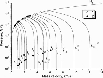
Figure 11 illustrates the expansion process in which, according to the present EOS, shocked aluminum is liquid. Again, EOS calculations are compared against experimental isentropes (Glushak et al., Reference Glushak, Zharkov, Zhernokletov, Ternovoi, Filimonov and Fortov1989; Knudson et al., Reference Knudson, Asay and Deeney2005). At higher pressure one can see from Figures 10 and 11 that the calculated isentropes s 15–s 21 deviate from the experimental data for expansion into air (Bakanova et al., Reference Bakanova, Dudoladov, Zhernokletov, Zubarev and Simakov1983; Glushak et al., Reference Glushak, Zharkov, Zhernokletov, Ternovoi, Filimonov and Fortov1989) in a non–systematic way. In contrast, the agreement with isentropes s 22–s 31 expanded into aerogel (Knudson et al., Reference Knudson, Asay and Deeney2005) is very good, see Figure 11. Like isentropes s 1–s 16 from Figure 10, all the isentropes s 17–s 31 show a monotonic dependence at all investigated pressures.
Release isentropes of liquid aluminum. Nomenclature: lines–EOS calculations, H 1–principal Hugoniot, s i–release isentropes; points–experiment, 1–expansion into air Glushak et al. (Reference Glushak, Zharkov, Zhernokletov, Ternovoi, Filimonov and Fortov1989), 2–expansion into aerogel Kundson et al. (2005).

All the release isentropes for aluminum s 1–s 31 from experiments (Bakanova et al., Reference Bakanova, Dudoladov, Zhernokletov, Zubarev and Simakov1983; Zhernokletov et al., Reference Zeldovich and Raizer1995; Glushak et al., Reference Glushak, Zharkov, Zhernokletov, Ternovoi, Filimonov and Fortov1989; Knudson et al., Reference Knudson, Asay and Deeney2005) are presented in Figure 12. It is interesting to note, the positions of these release isentropes in the phase space. In the experiments of Bakonova et al. (1983) and Zhernokletov et al. (Reference Zeldovich and Raizer1995), isentropes s 1–s 7 and s 10–s 12 are in the solid state, isentropes s 8 and s 13 originate in the solid state and end in the melting region, while the isentrope s 14 starts in the solid and ends in the liquid. Isentropes s 15–s 16 are mainly in the liquid state. Higher shock pressures, and consequently higher entropies, achieved in the experiments of Glushak et al. (Reference Glushak, Zharkov, Zhernokletov, Ternovoi, Filimonov and Fortov1989) and Knudson et al. (Reference Knudson, Asay and Deeney2005) result in all isentropes s 17–s 31 occupying a region of the liquid state. The analysis of the position of the two-phase liquid-gas region with respect to the shock adiabat of air, see line R and points in Figure 12, shows that aluminum does not and will not evaporate upon adiabatic expansion from shocked states into air.
Pressure–entropy diagram for aluminum. Nomenclature: lines–EOS calculations, H 1–principal Hugoniot, M–melting region, R–liquid–gas region with the critical point CP, s i–release isentropes (see Figs. 10, 11); points–experiment, 1–Zhernokletov et al. (Reference Zeldovich and Raizer1995), 2–Bakanova et al. (Reference Bakanova, Dudoladov, Zhernokletov, Zubarev and Simakov1983), 3–Glushak et al. (Reference Glushak, Zharkov, Zhernokletov, Ternovoi, Filimonov and Fortov1989), 4–Knudson et al. (Reference Knudson, Asay and Deeney2005).

Density measurements at P = 1 bar are available for solid (Toloukian et al., Reference Toloukian, Kirby, Taylor and Desay1975) and liquid (Lang, Reference Lang and Lide1995) aluminum at lower densities. Thermophysical properties of the liquid aluminum have been studied at P = 0.3 GPa in an isobaric expansion experiment (Gathers, Reference Gathers1983). EOS calculations are compared against these data and different evaluations of the critical point in Figure 13. This figure demonstrates that the present EOS describes the experimental points with outstanding accuracy. The EOS parameters of the critical point, P c = 0.197 GPa, T c = 6250 K, and V c = 1.423 cm3/g, agree with QEOS parameters P c = 0.168 GPa, T c = 5520 K (Young & Corey, Reference Young and Corey1995) and are also very closely in density with the other evaluations. This position of the critical point in the present EOS provides for an accurate description of IEX data (Gathers, Reference Gathers1983), see the 0.3 GPa isobar in Figure 13. The calculated evaporation temperature at room pressure, T V = 2770 K, coincides with the tabulated value (Hultrgen et al., Reference Hultrgen, Desai, Hawkins, Gleiser, Kelley and Wagman1973).
Phase diagram of aluminum at lower densities. Nomenclature: lines–EOS calculations, M–melting region, R–liquid-gas region with the critical point CP, P–isobars, and L–density of liquid metal at 1 bar Lang (1994–1995); points–experiment, 1–Toloukian et al. (Reference Toloukian, Kirby, Taylor and Desay1975), 2–Gathers (Reference Gathers1983), and evaluations of the critical points, 3–Gates & Thodos (Reference Gates and Thodos1960), 4–Morris (Reference Morris1964), 5–Young & Alder (Reference Young and Alder1971), 6–Fortov & Yakubov (Reference Fortov and Yakubov1999), 7–Gathers (Reference Gathers1986), 8–this work, 9–Likalter (Reference Likalter2002).

EOS isotherms are compared with QMD calculations (Desjarlais, personal communication) in Figure 14. The EOS critical isotherm at T = 6250 K describes the QMD results very well; the density of the critical point is also very close to the QMD result. The isotherm at T = 12000 K also shows good agreement with the QMD calculations.
Pressure–density diagram of aluminum's critical region. Nomenclature: lines–EOS calculations, R–liquid–gas region with the critical point CP, T–isotherms; open circles–QMD calculations Desjarlais (2006).

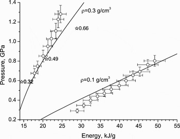
Experimental isochors of heated aluminum (Renaudin et al., Reference Renaudin, Blancard, Clerouin, Faussurier, Noiret and Recoules2003) occupy the super critical domain on the phase diagram. EOS isochors and the isochore 0.1 g/cm3 from Saha plasma model (Gryaznov et al., Reference Gryaznov, Fortov, Zhernokletov, Simakov, Trunin, Trusov and Iosilevski1998) are drawn in Figure 15, together with experimental points. The comparison with other advanced theoretical models is also available in the original work (Renaudin et al., Reference Renaudin, Blancard, Clerouin, Faussurier, Noiret and Recoules2003).
Pressure–energy diagram of isochorically heated aluminum. Nomenclature: lines–EOS calculations, points with bars–EPI experiment Renaudin et al. (Reference Renaudin, Blancard, Clerouin, Faussurier, Noiret and Recoules2003), open stars–Saha model Gryaznov et al. (Reference Gryaznov, Fortov, Zhernokletov, Simakov, Trunin, Trusov and Iosilevski1998) (numbers near stars indicate ionization ratio).
Finally, the summary of all mentioned above experimental data is given in 3D pressure–volume–temperature surface in Figure 16. It is worth to underline good potential capabilities of intense heavy ion beams for inducing high-energy-density states in expanded aluminum. In this region of practical interest and importance, we have today limited amount of a data for testing and calibrating modern theoretical models.
Generalized 3D volume-temperature-pressure surface for aluminum. M–melting region; R–boundary of two-phase liquid-gas region with the critical point CP; H 1 and H p–principal and porous Hugoniots; H air and H aerogel – shock adiabats of air and aerogel; DAC–diamond-anvil-cells data; ICE–isentropic compression experiment; IEX–isobaric expansion data; S–release isentropes; HIHEX–region accessible with use of intense heavy ion beams SIS18 and SIS100 (see for details Hoffman et al. (Reference Hoffmann, Fortov, Lomonosov, Mintsev, Tahir, Varentsov and Wieser2002); Tahir et al. (Reference Tahir, Deutsch, Fortov, Gryaznov, Hoffmann, Kulish, Lomonosov, Mintsev, Ni, Nikolaev, Piriz, Shilkin, Spiller, Shutov, Temporal, Ternovoi, Udrea and Varentsov2005a)). Phase states of the metal are also shown.

5. CONCLUSION
New advanced studies of aluminum properties at extreme conditions include experiments and theoretical calculations. Experimental investigations of isothermal, shock and isentropic compression of aluminum at high pressures up to 500 GPa have demonstrated behavior that results in a more “stiff” compression curve and shock adiabat for aluminum than was previously figured. Adiabatic-expansion measurements of shocked aluminum have brought new accurate data for the hot expanded liquid. Theoretical “ab initio” QMD calculations in the vicinity of the critical point have established the reference domain of thermodynamic data.
These data serve as a fundamental basis for the new multi-phase EOS for aluminum presented in this paper. It accounts for the high pressure, high temperature experimental, and theoretical data that was available up to the middle of 2007. The compression curve and the principal Hugoniot in the resulting EOS are fit to new data, as well as the critical point. According to the EOS model, shocked aluminum melts at 113 GPa and the parameters of the critical point are: P c = 0.197 GPa, T c = 6250 K, and V c = 1.423 cm3/g.
The developed EOS describes with high accuracy and reliability a broad range of the phase diagram, from the high-pressure shocked metal to more dense states in reflected shock waves and to regions of the phase diagram with much lower densities accessed in the process of the adiabatic expansion of shocked metal. The high accuracy suits this EOS to be applied in advanced numerical modeling for solving numerous problems in the physics of high energy densities. The developed EOS together with QMD data provides for self-consisted description of both thermodynamic and transport properties of aluminum.
Acknowledgments
We acknowledge Dr. M. P. Desjarlais for discussions and presented QMD-data and Dr. V. K. Gryaznov for results of Saha EOS calculations. The work was performed by support from Visiting Research Scholars Program at Sandia National Laboratories. Sandia is a multiprogram laboratory operated by Sandia Corporation, a Lockheed Martin Company, for the United States Department of Energy's National Nuclear Security Administration under contract DE-AC04-94AL85000.
APPENDIX EOS DATA
These tables present EOS coefficientsFootnote 2 as well as calculations of isotherms and the principal shock adiabat.Footnote 3 For more details, such as units, see also section Nomenclature.
EOS coefficients

T =0 K Isotherm

T =293 K Isotherm

Principal Hugoniot (here T is in 1000 K)


