


1. Introduction
The French credit life insurance market is dynamic and highly competitive. Although credit life insurance is not compulsory, it is commonly required by banks as a condition to obtain financing. Its primary goal is to protect policyholders, as well as lending institutions such as banks. This insurance is typically underwritten as a term life policy, with the term matching the duration of the credit, and it guarantees the repayment of all or part of the credit upon the occurrence of a covered risk (such as death, short-term and long-term disability, or, less commonly, unemployment). This market has seen significant changes and developments, particularly with recent legislative amendments aimed at improving consumer protection and market transparency. The most notable legislative change in recent years is the implementation of the Lemoine Law (Loi Lemoine), enacted at the beginning of 2022. One of the most important changes introduced by this law is the reduction of the so-called “right to forget” period, from ten to five years, for certain medical conditions. Concretely, individuals who have been in remission or cured for five years no longer need to declare their previous condition when applying for new credit life insurance policies. Moreover, the law mandates that insurers cannot collect health information or conduct medical examinations for mortgage loans if the insured amount is below EUR 200,000, and if the borrower’s age at the end of the loan period is under 60 years of age. Another notable change introduced by this law is the possibility of changing mortgage loan insurance at any time of the year. This “Résiliation Infra-Annuelle” (RIA) clause allows borrowers to cancel or lapse their insurance policy at any time of the year and replace it with another offer of equivalent coverage, regardless of how long they have held the policy.
Although these changes aim at improving consumer rights and increasing competition in the market, they also create new challenges for insurance companies. The consequences on insurance portfolios may be multiple, given the arbitrage possibilities for policyholders to switch coverage at any time of the year. These challenges are exacerbated when individuals with an aggravated state of health change insurance providers, as they do not need to disclose their medical history. With the use of the RIA clause, policyholders who were previously accepted with loading or with partial coverage can now replace their existing contract without going through a new selection process. This arbitrage opportunity can have a material impact on the profitability of an insurance company, as the clause skews lapse behavior. Projected and realized cash flows may diverge, particularly if many healthy policyholders leave and individuals with aggravated conditions become ones, introducing an information asymmetry that challenges traditional projection models.
Many studies investigate how policyholder and contract characteristics, together with external macroeconomic factors, affect lapse rates. In Kuo et al. (Reference Kuo, Tsai and Chen2003), a co-integrated vector autoregression model is employed to study two competing explanations for lapse rates. These are the emergency fund hypothesis and the interest rate hypothesis. Both of these propose that policyholders are likely to lapse whenever the market interest rate makes financial assets more attractive than policies, or whenever policyholders are facing financial hardships. The results of Kuo et al. (Reference Kuo, Tsai and Chen2003) highlight some variables that are believed to strongly influence lapses. Among these, they show that the unemployment rate influences lapses in both the short and long run, suggesting initial support for the emergency fund hypothesis. However, their impulse response analysis reveals that interest rates exert a more substantial overall impact on lapse rate dynamics, thus favoring the interest rate hypothesis in terms of economic significance. Using logistic regression and data from 133 German life insurers, Kiesenbauer (Reference Kiesenbauer2012) also examines how macroeconomic factors and policy characteristics influence lapse rates across five product categories. While the main determinants of lapse remain similar across most products, their impact on unit-linked policies differs significantly. Specifically, they find that the interest rate and emergency fund hypotheses apply only to unit-linked products, not to the other policy categories. In Russell et al. (Reference Russell, Fier, Carson and Dumm2013), life insurance data are employed to explore whether lapses or surrenders are driven by macroeconomic variables, thus possibly exhibiting strong correlations across policies. Their findings confirm both the emergency fund hypothesis and the interest rate hypothesis and further highlight a significant connection to the policy replacement hypothesis, demonstrating how economic conditions and policy replacement influence surrender behavior simultaneously. In Eling and Kiesenbauer (Reference Eling and Kiesenbauer2014), the authors consider life insurance contracts from a German insurance company, reflecting two periods of market turmoil. They employ proportional hazards and generalized linear models to investigate how both product and policyholder characteristics influence lapses. They conclude that factors such as product type, contract age, policyholder age, and gender are key drivers of lapse behavior. A competing risk framework is adopted in Milhaud and Dutang (Reference Milhaud and Dutang2018), to address how to better model policyholder surrender behavior in life insurance. Through back-testing, this approach aligns closely with observed lapse rates and facilitates the creation of experimental lapse tables, which can help insurers design products and manage lapse risk more effectively. A recent contribution on lapse modeling provides tree-based strategies with competing risks (Valla et al. Reference Valla, Milhaud and Olympio2024); see also Milhaud (Reference Milhaud2013) for a discussion of drivers of surrender risk.
In Loisel et al. (Reference Loisel, Piette and Tsai2021), two machine learning techniques are employed to model lapse risk under an economic capital framework by integrating solvency measures into their predictive models. A Lasso-based approach is considered in Reck et al. (Reference Reck, Schupp and Reuÿ2023), where the authors use sub-penalties for individual covariates to efficiently identify hidden structures in a life insurance portfolio and produce an interpretable lapse model for Solvency II valuation. Unlike random forests or neural networks, the Lasso method maintains full explainability by offering coefficient estimates that clarify the drivers of lapse risk at the contract level. Using data from a European life insurer, the authors show how the approach automatically calibrates lapse rates and improves the accuracy and transparency of risk assessment. Finally, Lobo et al. (Reference Lobo, Fonseca and Alves2024) propose a Bayesian survival model with mixture regressions to capture lapse rates observed in the initial months of life insurance contracts. An expectation-maximization (EM) algorithm is offered as an alternative, which uses both simulation and real-world data to illustrate how the model flexibly handles high proportions of censored observations.
Similarly to the abovementioned studies, the present work aims to analyze how both policy and policyholder characteristics, as well as macroeconomic variables, affect the lifetime of a credit life insurance contract. Instead of considering aggregated lapse rates, we estimate specific policy lifetime distributions using real data from the French credit life insurance market. Close attention will be given to understanding how these drivers affect the estimated distributions and their economic interpretation.
To this end, we adapt the proportional intensities (PI) model based on inhomogeneous phase-type (IPH) distributions introduced in Albrecher et al. (Reference Albrecher, Bladt, Bladt and Yslas2022a). This methodology is attractive as it yields flexible yet parsimonious survival models, while providing natural insights into the underlying aging process of the modeled lifetimes. Moreover, unlike most regression-based methods, this framework does not focus on estimating a single moment of a probability distribution, but the entire (conditional) distribution itself. Thus, the results of the PI model can be employed with any insurance product based on lifetime distributions, such as term life insurance or annuities, or to build lapse tables (similarly to Milhaud and Dutang Reference Milhaud and Dutang2018).
Examples of the flexibility provided by IPH distribution can be found in multiple manuscripts. In Albrecher et al. (Reference Albrecher, Bladt and Yslas2022b), a bivariate class of IPH distribution is employed to model Danish fire insurance data. Other noteworthy examples of how IPH distributions and covariate information can be used in nonlife insurance are given in Bladt and Yslas (Reference Bladt and Yslas2023a) and (Reference Bladt and Yslas2023b). Here, the authors introduce a mixture-of-experts (MoE) approach to embed covariate information into the initial distribution vector of IPH distributions, along with real-world data applications of the proposed methodology. They focus on severity modeling for a French Third Party Liability dataset and claim frequency modeling for the Wisconsin Local Government Property Insurance Fund data, respectively. Regarding survival analysis, Albrecher et al. (Reference Albrecher, Bladt, Bladt and Yslas2022a) use the same framework considered in the present manuscript to study female mortality data from Denmark, Japan, and the USA. Additionally, Albrecher et al. (Reference Albrecher, Bladt and Müller2023) analyze how couples’ ages affect joint lifetime distributions with multivariate IPH distributions using the MoE framework. The present paper contributes by (i) adapting the PI–IPH estimation framework to right-censored credit life data with shrinkage, (ii) documenting how borrower- and macro-level covariates jointly shape the full distribution of lapse times in a large French portfolio, and (iii) providing interpretable effect summaries via partial derivatives that relate covariates to timing of lapses.
The structure of the remainder of the paper is as follows. Section 2 introduces the underlying mechanics of IPH distributions and their PI extension. An adapted EM algorithm for feature selection and censored data is also proposed. Section 3 describes the data at our disposal, while the results of the model are found in Section 4. Particular focus is given to the interpretation of noteworthy variables such as the remaining sum insured, interest rates, and other economic variables found to increase lapse risk. Section 5 describes one possible way to concretely use the results of the PI model, if information on surrender values complements the data. Finally, Section 6 concludes.
2. Inhomogeneous phase-type distributions
Let
 $\{ J_t \}_{t \geq 0}$
denote a time-inhomogeneous Markov jump process on a finite state-space
$\{ J_t \}_{t \geq 0}$
denote a time-inhomogeneous Markov jump process on a finite state-space
 $\{1, \dots,$
 $p, p+1\}$
, where states
$p, p+1\}$
, where states
 $1,\dots,p$
are transient and state
$1,\dots,p$
are transient and state
 $p+1$
is absorbing. We assume that
$p+1$
is absorbing. We assume that
 $ \{ J_t \}_{t \geq 0}$
has an intensity matrix of the form
$ \{ J_t \}_{t \geq 0}$
has an intensity matrix of the form
 \begin{align*} \boldsymbol{\Lambda}(t)= \left( \begin{array}{cc} {\boldsymbol{T}}(t) & {\boldsymbol{t}}(t) \\ \boldsymbol{0} & 0 \end{array} \right)\in\mathbb{R}^{(p+1)\times(p+1)}, \quad t\geq0,\end{align*}
where
 ${\boldsymbol{T}}(t) $
is a
${\boldsymbol{T}}(t) $
is a
 $p \times p$
matrix function and
$p \times p$
matrix function and
 ${\boldsymbol{t}}(t)$
is a p-dimensional column vector function. Here, for any time
${\boldsymbol{t}}(t)$
is a p-dimensional column vector function. Here, for any time
 $t\geq0$
,
$t\geq0$
,
 ${\boldsymbol{t}} (t)=- {\boldsymbol{T}}(t) \, {\boldsymbol{e}}$
, where
${\boldsymbol{t}} (t)=- {\boldsymbol{T}}(t) \, {\boldsymbol{e}}$
, where
 ${\boldsymbol{e}} $
is the p-dimensional column vector of ones. Let
${\boldsymbol{e}} $
is the p-dimensional column vector of ones. Let
 $ \pi_{k} = {\mathbb P}(J_0 = k)$
,
$ \pi_{k} = {\mathbb P}(J_0 = k)$
,
 $k = 1,\dots, p$
,
$k = 1,\dots, p$
,
 $\boldsymbol{\pi} = (\pi_1 ,\dots,\pi_p )$
be a probability vector corresponding to the initial distribution of the jump process. We say that the time until absorption
$\boldsymbol{\pi} = (\pi_1 ,\dots,\pi_p )$
be a probability vector corresponding to the initial distribution of the jump process. We say that the time until absorption
 \begin{align*} \tau = \inf \{ t \geq 0 \mid J_t = p+1 \}\end{align*}
is inhomogeneous phase-type (IPH) distributed with representation
 $(\boldsymbol{\pi},{\boldsymbol{T}}(t))$
. We assume
$(\boldsymbol{\pi},{\boldsymbol{T}}(t))$
. We assume
 ${\mathbb P}(J_0 = p + 1) = 0$
, such that immediate absorptions are impossible. This assumption is not restrictive and is justified by the application of the present paper. Moreover, we only consider matrices of type
${\mathbb P}(J_0 = p + 1) = 0$
, such that immediate absorptions are impossible. This assumption is not restrictive and is justified by the application of the present paper. Moreover, we only consider matrices of type
 ${\boldsymbol{T}}(t) = \lambda(t)\,{\boldsymbol{T}}$
, where
${\boldsymbol{T}}(t) = \lambda(t)\,{\boldsymbol{T}}$
, where
 $\lambda(t)$
is some known nonnegative real function, named the intensity function. The matrix
$\lambda(t)$
is some known nonnegative real function, named the intensity function. The matrix
 ${\boldsymbol{T}}=\{t_{kl}\}_{1\le k,l\le p}$
is then called the sub-intensity matrix. Similarly, we let
${\boldsymbol{T}}=\{t_{kl}\}_{1\le k,l\le p}$
is then called the sub-intensity matrix. Similarly, we let
 $-{\boldsymbol{T}}{\boldsymbol{e}} ={\boldsymbol{t}}=\{t_k\}_{1\le k\le p}$
. For this particular case, we write
$-{\boldsymbol{T}}{\boldsymbol{e}} ={\boldsymbol{t}}=\{t_k\}_{1\le k\le p}$
. For this particular case, we write
 $$\tau \sim \mbox{IPH}(\boldsymbol{\pi} , {\boldsymbol{T}} , \lambda ).$$
This IPH representation yields explicit likelihood expressions and EM updates, and it provides the Markov interpretation that underlies the PI regression model introduced next.
Note that for
 $\lambda(t) \equiv 1$
one returns to the time-homogeneous case, which corresponds to the conventional phase-type distributions with notation
$\lambda(t) \equiv 1$
one returns to the time-homogeneous case, which corresponds to the conventional phase-type distributions with notation
 $\mbox{PH}(\boldsymbol{\pi} , {\boldsymbol{T}} )$
; a comprehensive account of PH distributions can be found in Bladt and Nielsen (Reference Bladt and Nielsen2017). It is not difficult to show that if
$\mbox{PH}(\boldsymbol{\pi} , {\boldsymbol{T}} )$
; a comprehensive account of PH distributions can be found in Bladt and Nielsen (Reference Bladt and Nielsen2017). It is not difficult to show that if
 $Y \sim \mbox{IPH}(\boldsymbol{\pi} , {\boldsymbol{T}} , \lambda )$
, then there exists a function g such that
$Y \sim \mbox{IPH}(\boldsymbol{\pi} , {\boldsymbol{T}} , \lambda )$
, then there exists a function g such that
 \begin{equation}{Y \stackrel{d}{=} g(Z)} ,\end{equation}
where
 $Z \sim \mbox{PH}(\boldsymbol{\pi} , {\boldsymbol{T}} )$
. Specifically, g is defined in terms of
$Z \sim \mbox{PH}(\boldsymbol{\pi} , {\boldsymbol{T}} )$
. Specifically, g is defined in terms of
 $\lambda$
by
$\lambda$
by
 \begin{equation*}g^{-1}(y) = \int_0^y \lambda (s)ds , \quad y\ge 0. \end{equation*}
or equivalently
 \begin{equation*}\lambda (y) = \frac{d}{dy}g^{-1}(y) . \end{equation*}
To avoid degeneracies, it is assumed that
 $g^{-1}(y)\lt\infty,\:\forall y\ge0$
, and
$g^{-1}(y)\lt\infty,\:\forall y\ge0$
, and
 $\lim_{y\to\infty}g^{-1}(y)=\infty$
. The density
$\lim_{y\to\infty}g^{-1}(y)=\infty$
. The density
 $f_Y$
and survival function
$f_Y$
and survival function
 $\overline{F}_Y$
of
$\overline{F}_Y$
of
 $Y \sim \mbox{IPH}(\boldsymbol{\pi} , {\boldsymbol{T}} , \lambda )$
are given by
$Y \sim \mbox{IPH}(\boldsymbol{\pi} , {\boldsymbol{T}} , \lambda )$
are given by
 \begin{eqnarray} f_Y(y) &=& \lambda (y)\, \boldsymbol{\pi}\exp \left( \int_0^y \lambda (s)ds\ {\boldsymbol{T}} \right){\boldsymbol{t}},\quad y\ge0 , \nonumber \\ \overline{F}_Y(y)&=& \boldsymbol{\pi}\exp \left( \int_0^y \lambda (s)ds\ {\boldsymbol{T}} \right){\boldsymbol{e}},\quad y\ge0 . \end{eqnarray}
For further properties on IPH distributions and motivation for their use in statistical modeling, we refer to Albrecher and Bladt (Reference Albrecher and Bladt2019). See also Albrecher et al. (Reference Albrecher, Bladt and Yslas2022b) for extensions to the multivariate case.
2.1 Proportional intensities model
To allow for more flexibility in the approximating IPH model, it is possible to take advantage of covariate information. This is achieved by letting the intensity function
 $\lambda(t)$
vary proportionally with the covariates. This assumption translates into each population subgroup having transition probabilities that are affected by a natural clock. This clock runs at a proportional speed with respect to other subgroups, the speed of which depends on the covariates. Moreover, this simple, yet powerful, specification allows a straightforward interpretation of the regression coefficients akin to the interpretation of coefficients in a generalized linear model (GLM). Note that in the following, the intensity function will not vary strictly proportionally to covariates. For ease of readability, we slightly abuse this term in the following.
$\lambda(t)$
vary proportionally with the covariates. This assumption translates into each population subgroup having transition probabilities that are affected by a natural clock. This clock runs at a proportional speed with respect to other subgroups, the speed of which depends on the covariates. Moreover, this simple, yet powerful, specification allows a straightforward interpretation of the regression coefficients akin to the interpretation of coefficients in a generalized linear model (GLM). Note that in the following, the intensity function will not vary strictly proportionally to covariates. For ease of readability, we slightly abuse this term in the following.
Using the framework introduced by Albrecher et al. (Reference Albrecher, Bladt, Bladt and Yslas2022a), we consider the proportional intensities (PI) regression model for IPH distributions. For a given distribution with representation
 $\mbox{IPH}(\boldsymbol{\pi} , {\boldsymbol{T}} , \lambda )$
, the intensity function now incorporates the predictor variables in
$\mbox{IPH}(\boldsymbol{\pi} , {\boldsymbol{T}} , \lambda )$
, the intensity function now incorporates the predictor variables in
 ${\boldsymbol{X}} = (X_1, \dots, X_d) \in \mathbb{R}^{n \times d}$
by specifying
${\boldsymbol{X}} = (X_1, \dots, X_d) \in \mathbb{R}^{n \times d}$
by specifying
 \begin{align} \lambda(t \mid {\boldsymbol{X}} , \boldsymbol{\theta} )=\lambda ( t;\; \boldsymbol{\theta} ) m({\boldsymbol{X}} \boldsymbol{\beta} ) ,\quad t\ge0,\end{align}
with
 $\boldsymbol{\theta}$
the parameter vector specific to the time-inhomogeneity distribution considered. Here,
$\boldsymbol{\theta}$
the parameter vector specific to the time-inhomogeneity distribution considered. Here,
 $ \boldsymbol{\beta}$
is a d-dimensional column vector and
$ \boldsymbol{\beta}$
is a d-dimensional column vector and
 $m(\!\cdot\!)$
is any positive-valued and measurable function. As stated before, the interpretation in terms of the underlying inhomogeneous Markov structure is that time is changed proportionally for a given subgroup when the associated PH distribution is transformed into an IPH one. In the sequel, we indistinctly denote by
$m(\!\cdot\!)$
is any positive-valued and measurable function. As stated before, the interpretation in terms of the underlying inhomogeneous Markov structure is that time is changed proportionally for a given subgroup when the associated PH distribution is transformed into an IPH one. In the sequel, we indistinctly denote by
 ${\boldsymbol{X}}$
a vector of covariates at the population level or a matrix of covariates for finite samples. In the latter case,
${\boldsymbol{X}}$
a vector of covariates at the population level or a matrix of covariates for finite samples. In the latter case,
 ${\boldsymbol{X}}_i$
denotes the ith row of the matrix, corresponding to the ith individual in the sample. We observe that both density f and survival function
${\boldsymbol{X}}_i$
denotes the ith row of the matrix, corresponding to the ith individual in the sample. We observe that both density f and survival function
 $\overline{F}$
of a random variable with distribution
$\overline{F}$
of a random variable with distribution
 $$ \mbox{IPH}(\boldsymbol{\pi} , {\boldsymbol{T}} , \lambda(\!\cdot\! | {\boldsymbol{X}} , \boldsymbol{\theta}) )$$
are very similar to (2.2), since they are given as
 \begin{eqnarray} f(y) &=& m({\boldsymbol{X}} \boldsymbol{\beta} ) \lambda (y;\; \boldsymbol{\theta})\, \boldsymbol{\pi}\exp \left( m({\boldsymbol{X}} \boldsymbol{\beta} )\int_0^y \lambda (s;\; \boldsymbol{\theta})ds\ {\boldsymbol{T}} \right)\!{\boldsymbol{t}}, \nonumber \\ \overline{F}(y)&=& \boldsymbol{\pi}\exp \left(m({\boldsymbol{X}} \boldsymbol{\beta} ) \int_0^y \lambda (s;\; \boldsymbol{\theta})ds\ {\boldsymbol{T}} \right)\!{\boldsymbol{e}}. \end{eqnarray}
Here, the role of the linear score
 $\boldsymbol{X}\boldsymbol{\beta}$
becomes apparent. The internal clock of the PI distribution affects the density function as if it were using a new sub-intensity matrix
$\boldsymbol{X}\boldsymbol{\beta}$
becomes apparent. The internal clock of the PI distribution affects the density function as if it were using a new sub-intensity matrix
 $m(\boldsymbol{X}\boldsymbol{\beta}) {\boldsymbol{T}}$
, which can vary for all subgroups of
$m(\boldsymbol{X}\boldsymbol{\beta}) {\boldsymbol{T}}$
, which can vary for all subgroups of
 ${\boldsymbol{X}}$
. Concretely, the modified transition probabilities lead to faster or slower absorptions (lifetimes) depending on the effect of predictors as reflected by
${\boldsymbol{X}}$
. Concretely, the modified transition probabilities lead to faster or slower absorptions (lifetimes) depending on the effect of predictors as reflected by
 $\boldsymbol{\beta}$
. Moreover, we observe that
$\boldsymbol{\beta}$
. Moreover, we observe that
 $m({\boldsymbol{X}}\beta)$
also multiplies the density function such that observations are now more, or less, likely to occur than before.
$m({\boldsymbol{X}}\beta)$
also multiplies the density function such that observations are now more, or less, likely to occur than before.
Within the above setup, it is also possible to add the dependence of g on
 ${\boldsymbol{X}}$
. That is, one may consider the model
${\boldsymbol{X}}$
. That is, one may consider the model
 \begin{align} \lambda(t \mid {\boldsymbol{X}} , \boldsymbol{\beta}, \boldsymbol{\gamma} )=\lambda (t;\; \boldsymbol{\theta}({\boldsymbol{X}}\boldsymbol{\gamma})) m({\boldsymbol{X}} \boldsymbol{\beta} ),\quad t\ge0,\end{align}
where
 $\boldsymbol{\theta}({\boldsymbol{X}}\boldsymbol{\gamma})$
becomes a vector-valued function, mapping the linear score
$\boldsymbol{\theta}({\boldsymbol{X}}\boldsymbol{\gamma})$
becomes a vector-valued function, mapping the linear score
 ${\boldsymbol{X}}\boldsymbol{\gamma}$
to the parameter space of
${\boldsymbol{X}}\boldsymbol{\gamma}$
to the parameter space of
 $\lambda$
. In this specification, the role of
$\lambda$
. In this specification, the role of
 $\boldsymbol{\theta}$
is to regulate the time-transformation of the underlying Markov dynamics. Incorporating covariates thus means that shortening or elongating virtual times is necessary to describe the differences observed in the data for individuals of the same subgroup, whose characteristics may differ nonetheless. In the sequel, any
$\boldsymbol{\theta}$
is to regulate the time-transformation of the underlying Markov dynamics. Incorporating covariates thus means that shortening or elongating virtual times is necessary to describe the differences observed in the data for individuals of the same subgroup, whose characteristics may differ nonetheless. In the sequel, any
 $\boldsymbol{\theta}$
specification may be of the form
$\boldsymbol{\theta}$
specification may be of the form
 $\boldsymbol{\theta}({\boldsymbol{X}}\boldsymbol{\gamma})$
, and the notation may be used interchangeably when there is no risk of confusion.
$\boldsymbol{\theta}({\boldsymbol{X}}\boldsymbol{\gamma})$
, and the notation may be used interchangeably when there is no risk of confusion.
Similarly to (2.1), an important property of the PI model is that a random variable following this specification can be expressed as a functional of a PH random variable. More specifically, consider
 $Y \sim \mbox{IPH}(\boldsymbol{\pi} , {\boldsymbol{T}} , \lambda(\!\cdot\! | {\boldsymbol{X}} , \boldsymbol{\beta}, \boldsymbol{\gamma}) )$
and let
$Y \sim \mbox{IPH}(\boldsymbol{\pi} , {\boldsymbol{T}} , \lambda(\!\cdot\! | {\boldsymbol{X}} , \boldsymbol{\beta}, \boldsymbol{\gamma}) )$
and let
 $g(\!\cdot \!|\, {\boldsymbol{X}}, \boldsymbol{\beta}, \boldsymbol{\gamma})$
be defined in terms of its inverse function
$g(\!\cdot \!|\, {\boldsymbol{X}}, \boldsymbol{\beta}, \boldsymbol{\gamma})$
be defined in terms of its inverse function
 $$g^{-1}(y \,|\, {\boldsymbol{X}}, \boldsymbol{\beta}, \boldsymbol{\gamma})=\int_{0}^{y}\lambda(s \,|\, {\boldsymbol{X}},\boldsymbol{\beta}, \boldsymbol{\gamma})ds = m({\boldsymbol{X}} \boldsymbol{\beta} )\int_{0}^{y}\lambda(s;\; \boldsymbol{\theta}({\boldsymbol{X}}\boldsymbol{\gamma}))ds,$$
Then it is not hard to see that
 \begin{align*} Y \stackrel{d}{=} g(Z\,|\, {\boldsymbol{X}},\boldsymbol{\beta}, \boldsymbol{\gamma}) ,\end{align*}
for any
 $Z\sim \mbox{PH}(\boldsymbol{\pi}, {\boldsymbol{T}})$
. Conversely,
$Z\sim \mbox{PH}(\boldsymbol{\pi}, {\boldsymbol{T}})$
. Conversely,
 \begin{align} Z=g^{-1}(Y \,|\, {\boldsymbol{X}}, \boldsymbol{\beta}, \boldsymbol{\gamma}) \sim \mbox{PH}(\boldsymbol{\pi} , {\boldsymbol{T}} ).\end{align}
This distributional property is a key observation for the estimation procedure proposed in the following Subsection 2.2.
2.2 Estimating PI distributions
We now present estimation via maximum likelihood (ML) for the PI model. We consider the estimation procedure for the general setting where the parameters of the inhomogeneity transform are also regressed, incurring no additional mathematical complexity.
In many real-world applications, a large proportion of the data is not entirely observed, or censored. The case of interval censoring arises naturally in the context of modeling the lifetime of a credit insurance contract with a fixed term. However, since we are interested in lapses, we favor the right-censored framework of the PI model. The reason originates in the interpretation of the model. If one would consider observations as interval censored, the upper bound of the interval would be seen as a time of lapse when, in reality, most of the policies are seen through their term. Moreover, this assumption could lead to a misinterpretation of the effect that covariates have on the estimated distribution. For example, all the policies that are close to their term would be considered close to a lapse, and the economic features at the time of observation might be wrongly identified as being relevant to the lapse occurring. To avoid this issue, we consider non-lapsed policies, which have not expired yet, as right-censored observations instead. This modeling choice solves the aforementioned problem, but another minor one remains. The estimated distributions may have positive mass beyond the term of the policy, which would introduce the possibility of having contract lifetimes that are larger than the term of the policy. This may be confusing at first, but an absorption occurring after the term of the contract can simply be interpreted as if a lapse would occur after the policy has expired. This artifact of IPH distributions can also be improved by introducing an atom at the time of maturity of a policy. This way, the probability of exceeding the term of the policy becomes null, and the behavior of the distribution until the policy maturity is not affected. Note that this adjustment is notable only for the distributions that have significant mass beyond the term. If a distribution already has a very small probability of surviving to maturity, the atom is negligible.
Regarding the estimation procedure, the main difference between the fully observed and right censored framework is that we no longer observe only exact data points
 $Y = y$
, but
$Y = y$
, but
 $Y \in [v,\infty)$
, conditionally on the corresponding covariate information. In particular, by monotonicity of g, we have that
$Y \in [v,\infty)$
, conditionally on the corresponding covariate information. In particular, by monotonicity of g, we have that
 $g^{-1}(Y;\; \boldsymbol{\theta} )\in ( g^{-1}(v;\;\boldsymbol{\theta} ), \infty)$
, which can be interpreted as a censored observation of a random variable with conventional PH distribution.
$g^{-1}(Y;\; \boldsymbol{\theta} )\in ( g^{-1}(v;\;\boldsymbol{\theta} ), \infty)$
, which can be interpreted as a censored observation of a random variable with conventional PH distribution.
Using notation from both Olsson (Reference Olsson1996), Albrecher et al. (Reference Albrecher, Bladt, Bladt and Yslas2022a), we present an adapted expectation-maximization (EM) algorithm for IPH distributions in the presence of covariates and right-censored data.
Let
 $(z_1,\delta_1), \dots, (z_N, \delta_N)$
be a possibly censored i.i.d. sample from of a PH distributed random variable Z with parameters
$(z_1,\delta_1), \dots, (z_N, \delta_N)$
be a possibly censored i.i.d. sample from of a PH distributed random variable Z with parameters
 $(\boldsymbol{\pi} , {\boldsymbol{T}} )$
, where the
$(\boldsymbol{\pi} , {\boldsymbol{T}} )$
, where the
 $\delta_i$
,
$\delta_i$
,
 $i=1,\dots,N$
are binary indicators taking the value 0 in case of censoring and 1 otherwise. Now, for each
$i=1,\dots,N$
are binary indicators taking the value 0 in case of censoring and 1 otherwise. Now, for each
 $k,l\in\{1,\dots,p\}$
, let
$k,l\in\{1,\dots,p\}$
, let
 $B_k$
be the number of times that the underlying jump-process
$B_k$
be the number of times that the underlying jump-process
 $(J_t)_{t\geq0}$
initiates in state k,
$(J_t)_{t\geq0}$
initiates in state k,
 $N_{kl}$
the total number of jumps from state k to l,
$N_{kl}$
the total number of jumps from state k to l,
 $N_k$
the number of times that we reach the absorbing state
$N_k$
the number of times that we reach the absorbing state
 $p+1$
from state k and let
$p+1$
from state k and let
 $V_k$
be the total time that the underlying Markov jump process spends in state k prior to absorption. These statistics are hidden, in the sense that Z alone cannot account for them. If they were not hidden, and given a sample of absorption times
$V_k$
be the total time that the underlying Markov jump process spends in state k prior to absorption. These statistics are hidden, in the sense that Z alone cannot account for them. If they were not hidden, and given a sample of absorption times
 ${\boldsymbol{z}}$
, the completely observed likelihood
${\boldsymbol{z}}$
, the completely observed likelihood
 $\mathcal{L}_c$
can be written in terms of these sufficient statistics as follows:
$\mathcal{L}_c$
can be written in terms of these sufficient statistics as follows:
 \begin{equation}\mathcal{L}_c( \boldsymbol{\pi} , {\boldsymbol{T}};\;{\boldsymbol{z}})=\prod_{k=1}^{p} {\pi_k}^{B_k} \prod_{k=1}^{p}\prod_{l\neq k} {t_{kl}}^{N_{kl}}e^{-t_{kl}V_k}\prod_{k=1}^{p}{t_k}^{N_k}e^{-t_{k}V_k},\end{equation}
which can be brought into the canonical form of the exponential dispersion family of distributions, which possess explicit maximum likelihood estimators.
However, since the full data are not observed, we employ the EM algorithm to obtain the ML estimators. At each iteration, the E-step consists of computing the conditional expectations of the sufficient statistics
 $B_k$
,
$B_k$
,
 $N_{kl}$
,
$N_{kl}$
,
 $N_k$
, and
$N_k$
, and
 $V_k$
given that
$V_k$
given that
 $Z=z$
, for the fully observed case, and given that
$Z=z$
, for the fully observed case, and given that
 $Z\in[v,\infty)$
for the right-censored case. The M-step maximizes
$Z\in[v,\infty)$
for the right-censored case. The M-step maximizes
 $\mathcal{L}_c( \boldsymbol{\pi} , {\boldsymbol{T}} ,{\boldsymbol{z}})$
using the estimates of the sufficient statistics from the previous step, obtaining updated parameters
$\mathcal{L}_c( \boldsymbol{\pi} , {\boldsymbol{T}} ,{\boldsymbol{z}})$
using the estimates of the sufficient statistics from the previous step, obtaining updated parameters
 $( \boldsymbol{\pi} , {\boldsymbol{T}} )$
.
$( \boldsymbol{\pi} , {\boldsymbol{T}} )$
.
Below we write the formulas needed for the E- and M-steps for a sample of size N. We denote by
 ${{\boldsymbol{e}}}_k$
the column vector with all elements equal to zero besides the kth entry, which is equal to one, that is, the kth element of the canonical basis of
${{\boldsymbol{e}}}_k$
the column vector with all elements equal to zero besides the kth entry, which is equal to one, that is, the kth element of the canonical basis of
 $\mathbb{R}^d$
. For completeness, the interval-censored case is given in Appendix A.
$\mathbb{R}^d$
. For completeness, the interval-censored case is given in Appendix A.
We now consider a sample of size N. For any two sets, A,B define their product
 $A\times B=\{(a,b)|\,a\in A,\,b\in B\}$
, with the definition extending inductively to the case of more than two sets. Define the following product set
$A\times B=\{(a,b)|\,a\in A,\,b\in B\}$
, with the definition extending inductively to the case of more than two sets. Define the following product set
 $\mathcal{Z}=\mathcal{Z}({\boldsymbol{z}})=\prod_{i=1}^N A_i$
, where
$\mathcal{Z}=\mathcal{Z}({\boldsymbol{z}})=\prod_{i=1}^N A_i$
, where
 $A_i=\{z_i\}$
if
$A_i=\{z_i\}$
if
 $\delta_i=1$
, and
$\delta_i=1$
, and
 $A_i=[z_i,\infty)$
otherwise. Then it can be shown that the conditional expectations can be written as follows:
$A_i=[z_i,\infty)$
otherwise. Then it can be shown that the conditional expectations can be written as follows:
-
(1) E-step, conditional expectations:
 \begin{align*} \mathbb{E}(B_k\mid {\boldsymbol{Z}}\in\mathcal{Z})=\sum_{i=1}^{N}\left\{ \delta_i\frac{\pi_k {{\boldsymbol{e}}_k}^{ \mathsf{T}}\exp( {\boldsymbol{T}} z_i) {\boldsymbol{t}} }{ \boldsymbol{\pi} \exp( {\boldsymbol{T}} z_i) {\boldsymbol{t}} }+(1-\delta_i)\frac{ \pi_{k} {\boldsymbol{e}}_{k}^{\mathsf{T}} \exp\left({\boldsymbol{T}} z_i\right){\boldsymbol{e}} } { \boldsymbol{\pi} \exp\left({\boldsymbol{T}} z_i\right){\boldsymbol{e}}}\right\},\end{align*}
\begin{align*} \mathbb{E}(V_k\mid{\boldsymbol{Z}}\in\mathcal{Z})&=\sum_{i=1}^{N} \left\{\delta_i\frac{\int_{0}^{z_i}{{\boldsymbol{e}}_k}^{ \mathsf{T}}\exp( {\boldsymbol{T}} (z_i-u)) {\boldsymbol{t}} \boldsymbol{\pi} \exp( {\boldsymbol{T}} u){\boldsymbol{e}}_kdu}{ \boldsymbol{\pi} \exp( {\boldsymbol{T}} z_i) {\boldsymbol{t}} } \right.\\ &\quad\quad \left. + (1-\delta_i)\frac{\int_{0}^{z_i}{{\boldsymbol{e}}_k}^{ \mathsf{T}}\exp( {\boldsymbol{T}} (z_i-u)) {\boldsymbol{e}} \boldsymbol{\pi} \exp( {\boldsymbol{T}} u){\boldsymbol{e}}_kdu}{ \boldsymbol{\pi} \exp( {\boldsymbol{T}} z_i) {\boldsymbol{e}} }\right\},\end{align*}
\begin{align*} \mathbb{E}(B_k\mid {\boldsymbol{Z}}\in\mathcal{Z})=\sum_{i=1}^{N}\left\{ \delta_i\frac{\pi_k {{\boldsymbol{e}}_k}^{ \mathsf{T}}\exp( {\boldsymbol{T}} z_i) {\boldsymbol{t}} }{ \boldsymbol{\pi} \exp( {\boldsymbol{T}} z_i) {\boldsymbol{t}} }+(1-\delta_i)\frac{ \pi_{k} {\boldsymbol{e}}_{k}^{\mathsf{T}} \exp\left({\boldsymbol{T}} z_i\right){\boldsymbol{e}} } { \boldsymbol{\pi} \exp\left({\boldsymbol{T}} z_i\right){\boldsymbol{e}}}\right\},\end{align*}
\begin{align*} \mathbb{E}(V_k\mid{\boldsymbol{Z}}\in\mathcal{Z})&=\sum_{i=1}^{N} \left\{\delta_i\frac{\int_{0}^{z_i}{{\boldsymbol{e}}_k}^{ \mathsf{T}}\exp( {\boldsymbol{T}} (z_i-u)) {\boldsymbol{t}} \boldsymbol{\pi} \exp( {\boldsymbol{T}} u){\boldsymbol{e}}_kdu}{ \boldsymbol{\pi} \exp( {\boldsymbol{T}} z_i) {\boldsymbol{t}} } \right.\\ &\quad\quad \left. + (1-\delta_i)\frac{\int_{0}^{z_i}{{\boldsymbol{e}}_k}^{ \mathsf{T}}\exp( {\boldsymbol{T}} (z_i-u)) {\boldsymbol{e}} \boldsymbol{\pi} \exp( {\boldsymbol{T}} u){\boldsymbol{e}}_kdu}{ \boldsymbol{\pi} \exp( {\boldsymbol{T}} z_i) {\boldsymbol{e}} }\right\},\end{align*}


 \begin{align*}\mathbb{E}(N_{kl}\mid{\boldsymbol{Z}}\in\mathcal{Z})&=\sum_{i=1}^{N}t_{kl} \left\{\delta_i \frac{\int_{0}^{z_i}{{\boldsymbol{e}}_l}^{\mathsf{T}}\exp( {\boldsymbol{T}} (z_i-u)) {\boldsymbol{t}} \, \boldsymbol{\pi} \exp( {\boldsymbol{T}} u){\boldsymbol{e}}_kdu}{ \boldsymbol{\pi} \exp( {\boldsymbol{T}} z_i) {\boldsymbol{t}} } \right.\\&\quad\quad \left.+ (1-\delta_i) \frac{\int_{0}^{z_i}{{\boldsymbol{e}}_l}^{\mathsf{T}}\exp( {\boldsymbol{T}} (z_i-u)) {\boldsymbol{e}} \, \boldsymbol{\pi} \exp( {\boldsymbol{T}} u){\boldsymbol{e}}_kdu}{ \boldsymbol{\pi} \exp( {\boldsymbol{T}} z_i) {\boldsymbol{e}} }\right\},\end{align*}
 \begin{align*}\mathbb{E}(N_k\mid {\boldsymbol{Z}}\in\mathcal{Z})=\sum_{i=1}^{N} \delta_it_k\frac{ \boldsymbol{\pi} \exp( {\boldsymbol{T}} z_i){{\boldsymbol{e}}}_k}{ \boldsymbol{\pi} \exp( {\boldsymbol{T}} z_i) {\boldsymbol{t}} }.\end{align*}
-
(2) M-step, explicit maximum likelihood estimators:
\begin{align*}\hat \pi_k=\frac{\mathbb{E}(B_k\mid {\boldsymbol{Z}}\in\mathcal{Z})}{N }, \quad \hat t_{kl}=\frac{\mathbb{E}(N_{kl}\mid {\boldsymbol{Z}}\in\mathcal{Z})}{\mathbb{E}(V_{k}\mid {\boldsymbol{Z}}\in\mathcal{Z})}\end{align*}
We set
\begin{align*}\hat t_{k}=\frac{\mathbb{E}(N_{k}\mid {\boldsymbol{Z}}\in\mathcal{Z})}{\mathbb{E}(V_{k}\mid {\boldsymbol{Z}}\in\mathcal{Z})},\quad \hat t_{kk}=-\sum_{s\neq k} \hat t_{ks}-\hat t_k.\end{align*}
$$ \hat{\boldsymbol{\pi}}=(\hat{\pi}_1, \dots,\: \hat{\pi}_p)^{},\quad \hat{{\boldsymbol{T}}} =\{{ \hat{t}}_{kl}\}_{k,l=1,2,\dots,p},\quad\hat{{\boldsymbol{t}}}=( \hat{t}_1,\dots,\: \hat{t}_p)^{\mathsf{T}}.$$


Note that the contributions from the conditional expectation of
 $N_{k}$
given that
$N_{k}$
given that
 $Z\gt z_i$
are zero, since absorption has not yet taken place. We refer to Albrecher et al. (Reference Albrecher, Bladt, Bladt and Yslas2022a), Section 4 for more details and numerical considerations when estimating PI models.
$Z\gt z_i$
are zero, since absorption has not yet taken place. We refer to Albrecher et al. (Reference Albrecher, Bladt, Bladt and Yslas2022a), Section 4 for more details and numerical considerations when estimating PI models.
For convenience, a summary of the entire procedure is provided in Algorithm 1. It is worth mentioning that the optimization problem in the fourth step of the EM procedure can be adapted to a weighted maximum likelihood estimation procedure. It suffices to multiply all logarithmic terms by the respective weights in the sample. This feature may be interesting when there is great uncertainty in the right-censored or interval-censored data. Depending on the range of the censoring interval, we may consider some observations more informative than others, particularly so when interval bounds are close to each other.
Another natural extension of the PI model consists of introducing a regularization term in the fourth step of Algorithm 1. Inspired by Tibshirani (Reference Tibshirani1996), the following constraint
 \begin{align} \mathcal{P}(\alpha_{\beta},\alpha_{\gamma}, \boldsymbol{\beta},\boldsymbol{\gamma}) &= \alpha_{\beta}{\|\boldsymbol{\beta}\|}_{k_\beta}+ \alpha_{\gamma}{\|{\boldsymbol{\gamma}}\|}_{k_\gamma}\\ &= \alpha_{\beta}\left( \sum_{j}^{d_\beta} \lvert \beta_j\rvert ^{k_\beta}\right)^{\frac{1}{k_\beta}}+\alpha_{\gamma}\left( \sum_{j}^{d_\gamma} \lvert \gamma_j \rvert^{k_\gamma}\right)^{\frac{1}{k_\gamma}},\nonumber\end{align}
can be subtracted from the log-likelihood given in the EM algorithm. Here,
 $\alpha_\beta$
and
$\alpha_\beta$
and
 $\alpha_\gamma$
are known parameters that set the weight of respective
$\alpha_\gamma$
are known parameters that set the weight of respective
 $l_{k_{\beta}}$
and
$l_{k_{\beta}}$
and
 $l_{k_{\gamma}}$
norms on the maximization problem. Note that
$l_{k_{\gamma}}$
norms on the maximization problem. Note that
 $d\beta$
and
$d\beta$
and
 $d\gamma$
denote the dimensions of the predictor vectors considered. Although d is the number of predictor variables, it is possible to only consider a subset of the variables in either
$d\gamma$
denote the dimensions of the predictor vectors considered. Although d is the number of predictor variables, it is possible to only consider a subset of the variables in either
 $\boldsymbol{\beta}$
or
$\boldsymbol{\beta}$
or
 $\boldsymbol{\gamma}$
.
$\boldsymbol{\gamma}$
.
Choosing
 $k_\beta = k_\gamma = 1$
and
$k_\beta = k_\gamma = 1$
and
 $\alpha_\beta = \alpha_\gamma = \alpha$
, we recover the least absolute shrinkage and selection operator (LASSO) introduced in Tibshirani (Reference Tibshirani1996). The LASSO can force some of the
$\alpha_\beta = \alpha_\gamma = \alpha$
, we recover the least absolute shrinkage and selection operator (LASSO) introduced in Tibshirani (Reference Tibshirani1996). The LASSO can force some of the
 $\widehat{\boldsymbol{\beta}}$
and
$\widehat{\boldsymbol{\beta}}$
and
 $\widehat{\boldsymbol{\gamma}}$
coefficient estimates to be exactly zero when the penalty is sufficiently large. This means LASSO not only reduces the influence of less important variables but can entirely remove them from the model. As a result, it provides a form of automatic feature selection, which can be very useful when dealing with a large number of covariates. Another alternative would be to use a Group LASSO approach (see Simon et al. Reference Simon, Friedman, Hastie and Tibshirani2013), when groups of variables should be excluded altogether.
$\widehat{\boldsymbol{\gamma}}$
coefficient estimates to be exactly zero when the penalty is sufficiently large. This means LASSO not only reduces the influence of less important variables but can entirely remove them from the model. As a result, it provides a form of automatic feature selection, which can be very useful when dealing with a large number of covariates. Another alternative would be to use a Group LASSO approach (see Simon et al. Reference Simon, Friedman, Hastie and Tibshirani2013), when groups of variables should be excluded altogether.
However, using a LASSO introduces an additional hyperparameter,
 $\alpha$
, that needs to be decided previous to running Algorithm 1. A common way to compare the effect of
$\alpha$
, that needs to be decided previous to running Algorithm 1. A common way to compare the effect of
 $\alpha$
on the estimation procedure is to perform a cross-validation study. Given different values of
$\alpha$
on the estimation procedure is to perform a cross-validation study. Given different values of
 $\alpha$
, the value leading to better performance is chosen. Here, performance refers to the observed-data (incomplete) log-likelihood evaluated on a validation sample, without including the penalty term in the evaluation. Because each fit is computationally costly, we use a simple hold-out split rather than a full k-fold scheme. Note that it would be possible to achieve better model performance with different penalization parameters. However, we do not follow this path as one needs to either arbitrarily choose these parameters, or perform a sensitivity analysis where both parameters vary simultaneously. The computational effort of the latter makes this option quite unattractive, while the former option requires expert judgment, which is what we try to avoid in the first place by introducing the penalization term.
$\alpha$
, the value leading to better performance is chosen. Here, performance refers to the observed-data (incomplete) log-likelihood evaluated on a validation sample, without including the penalty term in the evaluation. Because each fit is computationally costly, we use a simple hold-out split rather than a full k-fold scheme. Note that it would be possible to achieve better model performance with different penalization parameters. However, we do not follow this path as one needs to either arbitrarily choose these parameters, or perform a sensitivity analysis where both parameters vary simultaneously. The computational effort of the latter makes this option quite unattractive, while the former option requires expert judgment, which is what we try to avoid in the first place by introducing the penalization term.
Remark 2.1 As mentioned previously, the idea of the LASSO penalization is to not having to resort to expert judgment. We do not exclude the possibility that some variables influence only
 $m(\!\cdot\!)$
or
$m(\!\cdot\!)$
or
 $\lambda(\!\cdot\!)$
exclusively. Before the current version of the paper, we tried alternative configurations of both
$\lambda(\!\cdot\!)$
exclusively. Before the current version of the paper, we tried alternative configurations of both
 $m(\!\cdot\!)$
and
$m(\!\cdot\!)$
and
 $\lambda(\!\cdot\!)$
, where we decided arbitrarily which variable influences each term. However, these did not work as nicely as the current implementation. Our aim is to consider as many variables as possible, in order to identify the most relevant features that describe lapses. Nonetheless, the methodology presented can be easily adapted to have a simpler model formulation.
$\lambda(\!\cdot\!)$
, where we decided arbitrarily which variable influences each term. However, these did not work as nicely as the current implementation. Our aim is to consider as many variables as possible, in order to identify the most relevant features that describe lapses. Nonetheless, the methodology presented can be easily adapted to have a simpler model formulation.
Remark 2.2 The LASSO term only affects parameters that do not enter the EM. The “pure” EM algorithm is performed on the time-homogeneous samples obtained by transformation. Then, once both E and M steps are performed, the penalized maximum likelihood step happens. Therefore, the LASSO only affects the transformation of data into a time-homogeneous sample. This separation preserves the EM updates for
 $(\boldsymbol{\pi},{\boldsymbol{T}})$
while applying shrinkage only to
$(\boldsymbol{\pi},{\boldsymbol{T}})$
while applying shrinkage only to
 $(\boldsymbol{\beta},\boldsymbol{\gamma})$
.
$(\boldsymbol{\beta},\boldsymbol{\gamma})$
.
For readability, we repeat the key E- and M-step formulas in Algorithm 1 so that the procedure is self-contained.
Full EM algorithm for the Proportional Intensities (PI) model adapted to censoring and feature shrinkage.

3. French credit life insurance
In the following section, we take a closer look at the data we use in the application, starting with a short description of the data at our disposal.
3.1 Data exploration
The dataset we consider in this paper consists of 547,601 distinct policies, which are considered mutually independent from each other. Among all these policies, the expiry date is known for only 343,259 of them. There are 48,353 policies that are observed for the full duration of the contract, which we consider as right-censored, since they “experience” a lapse after the term of the policy has been reached. Note that this is an artefact of the framework we chose. As PH distributions are supported
 $\mathbb{R}^+$
and each contract has a fixed term, we ultimately consider a truncated version of the distribution estimated by Algorithm 1. This way, an atom of probability is introduced at the time of the end of a contract, indicating the probability of never lapsing.
$\mathbb{R}^+$
and each contract has a fixed term, we ultimately consider a truncated version of the distribution estimated by Algorithm 1. This way, an atom of probability is introduced at the time of the end of a contract, indicating the probability of never lapsing.
Regarding the remaining 294,906 policies, 145,376 of them experienced a lapse. Thus, we have an overall censoring rate of approximately 58%. Note that we have no information on whether a policy involves a surrender option, so we refer to both surrenders and lapses simply as lapses. Moreover, we do not know if any kind of administrative costs (or similar) are included when lapsing a contract.
All other ongoing policies that are not “lapsed” are also considered as being censored. We know that the contract lifetime survived at least until the observation time given in the dataset, but it can only survive further until the term of the contract. Remember that we consider these observations as right-censored, instead of interval-censored. We want to prevent this feature from skewing the interpretation of the coefficient estimated in the PI model. Assuming interval-censoring results in always observing a lapse, although it may happen exactly at the time of the expiry of the policy. Note that there are only a handful of policies where the “lapse” occurred because of the policyholder’s death. As this competing risk is noninformative in terms of lapse, these observations have been removed from our sample.
For each policy, information about both the policyholder and the contract is available, and these are summarized in Table 1. Note that in the dataset, some policyholders underwrote more than one policy. We assume that contracts held by the same individual are independent, in that only the policyholder and contract characteristics affect the time until a lapse occurs. Moreover, the dataset records the history of some contracts, and every time there is a change in the exposure, a new entry is created for the same policy. A more realistic yet more cumbersome approach would be to consider a multivariate setting for policies owned by the same individuals. However, for the sake of simplicity, we consider loans as independent from each other and only consider the most recent entry for each policy. Consequently, we choose not to use any variable that is adjusted by the number of policies held by an individual (e.g., claimLifeadj, exposureLifeadj, and isaPerson). Additionally, some of the covariates in Table 1 can reasonably be considered noninformative regarding the lifetime of a contract. For example, all variables whose sole purpose is to identify contracts are disregarded (e.g, insId, id, loanId), as are some variables with a very small number of observations. For instance, the variable claim indicates if the termination of the contract happened for a reason other than a lapse or surrender. Depending on the terms of the policy, this may happen if the policyholder dies or becomes disabled in the long term. As we are ultimately interested in voluntary lapses, we disregard these observations.
Description of all predictor variables present in the dataset. Variables in bold font are ultimately selected for the PI model. Variables in the bottom part of the table are computed from recorded variables.

3.2 Variable selection
Hereafter, we describe all predictor variables that are used in the PI model. Instead of considering the amount of time passed since issuance, we decided to focus on the proportion of contract lifetimes that passed until the time of observation. This choice is justified by the fact that the policies’ terms are quite heterogeneous, and it is not straightforward to compare contracts with different maturities. Thus, considering the proportion of observed contract lifetimes allows for a more natural interpretation of the results of the PI model proposed later on.
Regarding the policyholder’s characteristics, we consider age, sex, smoking status, and employment type. The following policy features are also selected as potential variables for the PI model. For each policy, we know the initial and current sum insured and the interest rate that applies to it. Additionally, we know the type of premium that individuals subscribe to, if a policy is sub-standard and the reason behind the loan. Both exposure and duration are strongly correlated with the contract lifetime. For this reason, we decided not to consider them as predictor values. Keeping them in the covariate set would mechanically reduce the predictive power of other features, which is undesirable.
Let us focus on the reasons why individuals ask for capital (variable loanReason in Table 1). The most common reason to subscribe to a loan in the data is for purchasing a principal residence (res_principale), followed by loans that cover expenses to buy real estate to rent it to others (locatif). The third most common reason why individuals get indebted is for consumption loans (pret_conso). These loans usually involve smaller capital, which can be used freely by the policyholder. The remaining loan reasons are loans for professional reasons, for secondary residences and renovation works. They all have similar frequency in the data, and along with consumption loans, they are much rarer than the first two categories. Given the unbalanced nature of the dataset, we disregard loan reasons if the number of fully observed lapses is very small (less than 30 observations).
For each individual, we are given an occupational risk class based on their line of work. These classes can be used as proxies of the policyholder’s lifestyle, social class, and likelihood of getting injured. We give a brief description of the three separate risk classes present in the data. The first class encompasses executive employees (excluding paramedical and teaching professions), liberal professionals (excluding craftsmen, shopkeepers, and paramedical professions) and medical professionals. Moreover, any of these professions should not involve any hazardous manual work or frequent business travel (business travel is considered frequent if it involves more than 20,000 km per year in a motorized vehicle, excluding planes and trains). In the second class, we find non-executive employees, teachers, paramedical professionals, craftsmen, and shopkeepers. Similarly to the first class, all these professions should not imply manual work or frequent business travel. In the third risk class, we find any profession that does not fit the other risk classes. Concretely, all individuals who perform hazardous manual work and/or have frequent business travels are put into that risk class. Note that in this context, hazardous manual work is defined as any work involving tools or machinery that could cause serious injuries to the individual. Furthermore, any line of work where manual labor is performed outdoors or implies carrying heavy objects is also categorized as hazardous manual labor. Thus, the occupational risk class captures the difference in purchasing power and possibly provides some information on the health status of a policyholder.
Finally, the other categorical variables that we have at our disposal are the type of premium that an individual pays (premiumType) and a sub-standard policy indicator (rated).
On top of information recorded by first-line insurers, three variables are considered to represent the economic cycle at the time of lapse or observation. These are the monthly annualized agreed interest rates concerning new loans for house purchases, the monthly mean unemployment rate, and the monthly mean inflation rate (source https://webstat.banque-france.fr/fr/#/home). According to the interest rate hypothesis, the market interest rate influences the lapse rate as the former can be interpreted as the opportunity cost for owning an insurance contract (see Kuo et al. Reference Kuo, Tsai and Chen2003). Moreover, a downward pressure on new policy prices may result from an increase in the market interest rate. This effect might play a major role in future lapses in the French credit life insurance market, as policyholders are now allowed to cancel their policy in exchange for another one, provided equivalent coverage. Both the unemployment and inflation rates, as well as the market interest rate, are used as proxies of economic growth. As mentioned previously, policyholders may lapse when facing personal financial distress. For example, policyholders may not be able to afford premiums any more, or they may want to exercise the surrender option to use the proceeds as an emergency fund. We believe that the nominal value of either agreed interest rates, inflation, and unemployment rates is not necessarily the driver of lapses. Instead, we assume that the relative economic cycle is more relevant in describing the lapsing behavior of an individual. Over time, both the personal and economic environment of policyholders can change drastically. For example, an individual who subscribed to a loan in the year 2015 may have changed her lifestyle completely. Moreover, since 2015, interest rates have slowly decreased until a sudden rise starting in 2022, leading to cheaper premiums for the same coverage (assuming that the same mortality applies) while rates decreased. The policyholder might be tempted to change her insurance provider, particularly if there are many years left in her contract. Moreover, if policyholders expect a decrease in the market interest rates, they might renegotiate their loans, which causes a lapse. This way, as insurance premiums become less expensive, the effective cost of the loan diminishes, making a change of insurance provider attractive. Thus, we consider relative changes in the interest rates between issuance and time of observation of a policy as a predictive variable. Moreover, both unemployment and inflation rates are also considered relative to the economic cycle at policy issuance. Consequently, these growth rates are used as proxies of the relative change in economic conditions since the issuance of the policy.
4. Modeling time to lapses with the PI model
In the following section, we describe the implementation of the methodology described previously. As mentioned before, we choose to consider the proportion of time that individuals spend in their contract as our variable of interest. This is motivated by the fact that comparing contracts of short and long terms may be misleading, as the impact they have on individuals’ lives may differ substantially depending on the duration of the insurance product. Moreover, we only present the results for one data portfolio. Accordingly, the contractual term is used only to scale observations into proportions and is not included as a predictor in the PI model.
Let the vector of independent contract lifetime proportions be denoted by
 ${\boldsymbol{Y}} = (Y_1,\dots, Y_N)^{\mathsf{T}}$
. It may seem weird at first that we consider a continuous distribution for data that is bounded in (0, 1). However, an eventual distribution mass beyond one can be thought of as the probability of never lapsing, that is to see a contract through. This introduces a “virtual” atom at infinity that leads to the possibility of never witnessing an absorption. This behavior is investigated in Bladt and Yslas (Reference Bladt and Yslas2024), where absorption is considered as an illness, while atoms are considered as “curing” states.
${\boldsymbol{Y}} = (Y_1,\dots, Y_N)^{\mathsf{T}}$
. It may seem weird at first that we consider a continuous distribution for data that is bounded in (0, 1). However, an eventual distribution mass beyond one can be thought of as the probability of never lapsing, that is to see a contract through. This introduces a “virtual” atom at infinity that leads to the possibility of never witnessing an absorption. This behavior is investigated in Bladt and Yslas (Reference Bladt and Yslas2024), where absorption is considered as an illness, while atoms are considered as “curing” states.
We assume that
 $Y_i \sim \mbox{IPH}(\boldsymbol{\pi},{\boldsymbol{T}}, \lambda(\cdot \mid {\boldsymbol{X}}_i,\boldsymbol{\beta},\boldsymbol{\gamma}))$
, where
$Y_i \sim \mbox{IPH}(\boldsymbol{\pi},{\boldsymbol{T}}, \lambda(\cdot \mid {\boldsymbol{X}}_i,\boldsymbol{\beta},\boldsymbol{\gamma}))$
, where
 ${\boldsymbol{X}}$
is the covariate matrix, with coefficients
${\boldsymbol{X}}$
is the covariate matrix, with coefficients
 $\boldsymbol{\beta}$
and
$\boldsymbol{\beta}$
and
 $\boldsymbol{\gamma}$
for the proportionality term and inhomogeneity function, respectively.
$\boldsymbol{\gamma}$
for the proportionality term and inhomogeneity function, respectively.
The shrinkage term in Algorithm 1 introduces an automatic feature selection. We therefore decide to use the same variables for both the proportionality and the inhomogeneity terms. This way, we do not need to decide which feature should be considered for either term, but let the LASSO shrink estimated coefficients to zero if required. Using all covariates in both terms also gives a contrasting interpretation of the importance of a feature on the IPH distribution. Recall that in the PI model, each risk class has a natural clock running at a proportional speed relative to other classes (modeled by the proportionality term). At the same time, the inhomogeneity term further accentuates these differences by changing the shape of the distribution. Thus, we can compare whether a given feature is more important in describing the proportional shift of the distribution or the shape of the distribution itself. Although the same covariates enter both terms, they act on different components of the model:
 $m({\boldsymbol{X}}\boldsymbol{\beta})$
rescales the internal clock, while
$m({\boldsymbol{X}}\boldsymbol{\beta})$
rescales the internal clock, while
 $\lambda(\cdot;\boldsymbol{\theta}({\boldsymbol{X}}\boldsymbol{\gamma}))$
changes the shape of the baseline inhomogeneity. In the matrix-Weibull case,
$\lambda(\cdot;\boldsymbol{\theta}({\boldsymbol{X}}\boldsymbol{\gamma}))$
changes the shape of the baseline inhomogeneity. In the matrix-Weibull case,
 $\boldsymbol{\beta}$
primarily affects a scale factor and
$\boldsymbol{\beta}$
primarily affects a scale factor and
 $\boldsymbol{\gamma}$
alters a shape parameter, so the two sets of effects are not collinear in the usual linear-predictor sense. The shrinkage term remains available to control redundancy when it is present.
$\boldsymbol{\gamma}$
alters a shape parameter, so the two sets of effects are not collinear in the usual linear-predictor sense. The shrinkage term remains available to control redundancy when it is present.
This modeling assumption combines both emergency fund and interest rate theories under the same framework. Effects of changes in interest rates on lapses are reflected by the coefficients associated with initial loan rates, market interest rates at the time of observation and their relative difference. On the other hand, the emergency fund theory is reflected by predictors that serve as proxies for the economic situation at the time of observation (e.g. the inflation rate and unemployment rate), as well as the characteristics of the policyholder. Thus, we may observe competing effects of such variables in the description of lapses, without needing to favor one over the other.
The ith proportional lifetime is assumed to be IPH distributed with shared representation
 $(\boldsymbol{\pi},{\boldsymbol{T}})$
and contract-specific intensity function given by
$(\boldsymbol{\pi},{\boldsymbol{T}})$
and contract-specific intensity function given by
 \begin{align*} \lambda(s \mid {\boldsymbol{X}}_i,\boldsymbol{\beta},\boldsymbol{\gamma})) &= m({\boldsymbol{X}}_i \boldsymbol{\beta})\lambda(s,\boldsymbol{\theta}({\boldsymbol{X}}_i\boldsymbol{\gamma}))\\ &=e^{{\boldsymbol{X}}_i \boldsymbol{\beta}}e^{{\boldsymbol{Y}}_{\boldsymbol{i}}\boldsymbol{\gamma}}s^{e^{{\boldsymbol{Y}}_{\boldsymbol{i}}\boldsymbol{\gamma}}-1},\end{align*}
where a column of ones is implicitly added to
 ${\boldsymbol{X}}$
to allow for a minimal degree of flexibility to the intensity function, particularly when
${\boldsymbol{X}}$
to allow for a minimal degree of flexibility to the intensity function, particularly when
 ${\boldsymbol{X}}_i \boldsymbol{\gamma}=0$
, as we need a positive inhomogeneity parameter (i.e.,
${\boldsymbol{X}}_i \boldsymbol{\gamma}=0$
, as we need a positive inhomogeneity parameter (i.e.,
 $\boldsymbol{\theta}({\boldsymbol{X}}_i\boldsymbol{\gamma})\gt 0$
). This choice of intensity function corresponds to a matrix-Weibull distribution. For more details on matrix distributions, refer to Albrecher and Bladt (Reference Albrecher and Bladt2019). The matrix-Weibull distribution was selected as it provides the best fit to the data among the available distributions in the matrixdist R package (see Bladt et al. Reference Bladt, Mueller and Yslas2025).
$\boldsymbol{\theta}({\boldsymbol{X}}_i\boldsymbol{\gamma})\gt 0$
). This choice of intensity function corresponds to a matrix-Weibull distribution. For more details on matrix distributions, refer to Albrecher and Bladt (Reference Albrecher and Bladt2019). The matrix-Weibull distribution was selected as it provides the best fit to the data among the available distributions in the matrixdist R package (see Bladt et al. Reference Bladt, Mueller and Yslas2025).
Regarding the common representation
 $(\boldsymbol{\pi}, {\boldsymbol{T}})$
, we choose a generalized Coxian structure of dimension
$(\boldsymbol{\pi}, {\boldsymbol{T}})$
, we choose a generalized Coxian structure of dimension
 $p = 5$
. This structure allows the underlying Markov jump process to start in any of the p states, but only transitions to the next state or the absorbing state are possible. The dimension
$p = 5$
. This structure allows the underlying Markov jump process to start in any of the p states, but only transitions to the next state or the absorbing state are possible. The dimension
 $p=5$
is fairly small, however, as confirmed later, it suffices to give a good approximation of the data. It would be possible to increase the number of states to improve the fit even further, but it would increase computational complexity without the assurance of substantially improving the distribution. The transient states can be interpreted as latent “ageing” stages that the contract passes through before a lapse occurs, while the absorbing state corresponds to lapse.
$p=5$
is fairly small, however, as confirmed later, it suffices to give a good approximation of the data. It would be possible to increase the number of states to improve the fit even further, but it would increase computational complexity without the assurance of substantially improving the distribution. The transient states can be interpreted as latent “ageing” stages that the contract passes through before a lapse occurs, while the absorbing state corresponds to lapse.
Depending on
 ${\boldsymbol{X}}_i$
, each contract lifetime may follow a different distribution. Thus, the common representation
${\boldsymbol{X}}_i$
, each contract lifetime may follow a different distribution. Thus, the common representation
 $(\boldsymbol{\pi}, {\boldsymbol{T}})$
sets the underlying phase-type transition mechanism, while the proportionality term and intensity function affect the “virtual clock” that determines when transitions happen. Then, for a given time, policyholders with heterogeneous attributes have different probabilities of lapsing their policy. Note that even if we talk about the survival probability of the time until a lapse occurs, the lapse might never occur. It can also be thought of as happening after the policy is seen through (by mathematical construction), which is the reason why we model such observations as right censored in the first place.
$(\boldsymbol{\pi}, {\boldsymbol{T}})$
sets the underlying phase-type transition mechanism, while the proportionality term and intensity function affect the “virtual clock” that determines when transitions happen. Then, for a given time, policyholders with heterogeneous attributes have different probabilities of lapsing their policy. Note that even if we talk about the survival probability of the time until a lapse occurs, the lapse might never occur. It can also be thought of as happening after the policy is seen through (by mathematical construction), which is the reason why we model such observations as right censored in the first place.
Before using Algorithm 1, all the continuous covariates are normalized as their magnitudes vary from one another. Namely, respective sample averages are subtracted from each covariate, which are then divided by their sample standard deviations. We want to prevent features with large magnitudes from dominating others in the intensity function just because of their cardinality and not their actual importance in the observed data. For example, the scale of the initial sum insured is in the thousands, while loan rates are percentages. As we are using a transformation of a linear score, it would not be wise to use covariates as such. Furthermore, this manipulation improves numerical stability when the maximum likelihood estimation is performed, particularly when gradient-based optimization algorithms are employed to find the optimal solution (which is our case). As a consequence, a sort of reference distribution is estimated by Algorithm 1.
The distribution of policyholders whose continuous covariates (e.g., age or sum insured) equal respective sample averages, and whose categorical covariates (such as sex, smoker status, or occupational class) fall into the most common categories observed in the data, can be considered as a baseline distribution with intensity function
 $\lambda(s \mid {\boldsymbol{X}}_i,\boldsymbol{\beta},\boldsymbol{\gamma}))=e^{\gamma_0}s^{e^{\gamma_0}-1}$
. Then, all other distributions vary from this reference case, according to the value of estimated coefficients in
$\lambda(s \mid {\boldsymbol{X}}_i,\boldsymbol{\beta},\boldsymbol{\gamma}))=e^{\gamma_0}s^{e^{\gamma_0}-1}$
. Then, all other distributions vary from this reference case, according to the value of estimated coefficients in
 $\boldsymbol{\beta}$
and
$\boldsymbol{\beta}$
and
 $\boldsymbol{\gamma}$
. To get an idea of how these coefficients affect the estimated distributions, we can observe the partial derivatives of the resulting densities, or for simplicity’s sake, the ones from the survival function.
$\boldsymbol{\gamma}$
. To get an idea of how these coefficients affect the estimated distributions, we can observe the partial derivatives of the resulting densities, or for simplicity’s sake, the ones from the survival function.
Assuming a matrix-Weibull reference distribution, the partial derivative with respect to the covariate k of policyholder i is
 \begin{align} \frac{\mathrm{d} \overline{F}_{Y_i}(y)}{\mathrm{d} X_{ik}}&=\frac{\mathrm{d}}{\mathrm{d} X_{ik}}\left[\boldsymbol{\pi}e^{{\boldsymbol{T}}e^{\boldsymbol{X}_{\boldsymbol{i}}\boldsymbol{\beta}+\log(y)e^{\boldsymbol{X}_{\boldsymbol{i}}\boldsymbol{\gamma}}}}{\boldsymbol{e}}\right]\\ &= -\left(\beta_k+\gamma_k\log(y)e^{\boldsymbol{X}_{\boldsymbol{i}}\boldsymbol{\gamma}} \right)e^{{\boldsymbol{X}_{\boldsymbol{i}}\boldsymbol{\beta}}+\log(y)e^{{\boldsymbol{X}_{\boldsymbol{i}}\boldsymbol{\gamma}}}}\boldsymbol{\pi}e^{{\boldsymbol{T}}e^{{\boldsymbol{X}_{\boldsymbol{i}}\boldsymbol{\beta}}+\log(y)e^{{\boldsymbol{X}_{\boldsymbol{i}}\boldsymbol{\gamma}}}}}{\boldsymbol{t}} \nonumber\\ &= -\left(\beta_k+\gamma_k\log(y)e^{{\boldsymbol{X}_{\boldsymbol{i}}\boldsymbol{\gamma}}} \right)f_{Y_i}(y)ye^{-{\boldsymbol{X}_{\boldsymbol{i}}\boldsymbol{\gamma}}} \nonumber\\ & = -\left(\beta_k+\gamma_kC_i^- \right)C_i^+, \quad C_i^+\ge 0,C_i^-\le 0.\nonumber\end{align}
We observe that if
 $sgn(\beta_k) \neq sgn(\gamma_k)$
, the partial derivative assumes a positive or negative value. However, when
$sgn(\beta_k) \neq sgn(\gamma_k)$
, the partial derivative assumes a positive or negative value. However, when
 $sgn(\beta_k) = sgn(\gamma_k)$
, the sign of the partial derivative depends on the estimated values as well as the argument y considered. Therefore, we need to evaluate (4.1) numerically to understand how changes in the covariates affect the distribution for policyholder i.
$sgn(\beta_k) = sgn(\gamma_k)$
, the sign of the partial derivative depends on the estimated values as well as the argument y considered. Therefore, we need to evaluate (4.1) numerically to understand how changes in the covariates affect the distribution for policyholder i.
4.1 Results for the anonymized portfolio
Next, we provide details on the estimation of the PI model for the data considered. We start by describing how to get a starting point for Algorithm 1, followed by a cross-validation study to determine the hyperparameter associated with the LASSO penalty. Then, we describe the results of the optimal PI model, focusing on the interpretation of estimated coefficients
 $\widehat{\beta}$
,
$\widehat{\beta}$
,
 $\widehat{\gamma}$
, as well as partial dependence plots.
$\widehat{\gamma}$
, as well as partial dependence plots.
4.1.1 Parametric estimation without covariate information
To improve numerical stability in Algorithm 1, we propose to estimate an IPH distribution with the characteristics mentioned above, but without any covariate information. Doing so, we get a more precise starting point in the estimation of the PI model. Moreover, we can compare the resulting approximating distribution with a non-parametric estimator of the survival function to check if the starting approximation is reasonable to begin with. Figure 1 provides a comparison of the IPH survival function with the Kaplan–Meier (KM) estimator (see Turnbull Reference Turnbull1974). We observe that the solid blue line (IPH approximation) closely follows the nonparametric estimator for the entirety of the distribution support. This indicates that the approximating distribution is capturing the behavior of the data when covariates are not considered. Moreover, we observe that the probability of surviving until the end of the contract is approximately 50%. For brevity, we do not report the full parameter table for
 $\left(\widehat{\boldsymbol{\pi}},\widehat{{\boldsymbol{T}}},\exp\left(\widehat{\gamma}_0\right)\right)$
; the Coxian parameters are not directly interpretable (matrix models are nonidentifiable) and would add substantial length. The estimated distribution depicted in Figure 1 is then used as the starting point of Algorithm 1. Namely, the estimated representation is used as the starting input of the estimation procedure.
$\left(\widehat{\boldsymbol{\pi}},\widehat{{\boldsymbol{T}}},\exp\left(\widehat{\gamma}_0\right)\right)$
; the Coxian parameters are not directly interpretable (matrix models are nonidentifiable) and would add substantial length. The estimated distribution depicted in Figure 1 is then used as the starting point of Algorithm 1. Namely, the estimated representation is used as the starting input of the estimation procedure.
Comparison between the Kaplan–Meier estimator (blue curve) and IPH model (red curve) without covariates.

Estimated coefficients for the unpenalized PI model.

4.1.2 Cross validation of shrinkage parameters
Once a common representation has been estimated, we can focus on finding a suitable value for
 $\alpha$
in the LASSO. We use a simple validation study where Algorithm 1 is fit on a training subset for increasing values of
$\alpha$
in the LASSO. We use a simple validation study where Algorithm 1 is fit on a training subset for increasing values of
 $\alpha$
, and we evaluate the observed-data (incomplete) log-likelihood on a hold-out validation set. Starting with the unpenalized model (
$\alpha$
, and we evaluate the observed-data (incomplete) log-likelihood on a hold-out validation set. Starting with the unpenalized model (
 $\alpha=0$
), we increase
$\alpha=0$
), we increase
 $\alpha$
linearly to determine which value yields the highest likelihood. Figure 2 shows the result of this study. The horizontal axis in Figure 2 corresponds to the grid of
$\alpha$
linearly to determine which value yields the highest likelihood. Figure 2 shows the result of this study. The horizontal axis in Figure 2 corresponds to the grid of
 $\alpha$
values considered in the search. We observe that the unpenalized model (
$\alpha$
values considered in the search. We observe that the unpenalized model (
 $\alpha=0$
) slightly outperforms the other models. The small dip at one grid point is consistent with a local optimum in the EM fit for that
$\alpha=0$
) slightly outperforms the other models. The small dip at one grid point is consistent with a local optimum in the EM fit for that
 $\alpha$
and does not alter the overall ranking. In this application, the data are sufficiently informative that shrinkage brings limited gains; nevertheless, we retain the LASSO machinery for stability and for settings with higher-dimensional or noisier covariate sets.
$\alpha$
and does not alter the overall ranking. In this application, the data are sufficiently informative that shrinkage brings limited gains; nevertheless, we retain the LASSO machinery for stability and for settings with higher-dimensional or noisier covariate sets.
Cross-validation log-likelihoods. The evolution of observed-data log-likelihoods is depicted for each
 $\alpha$
considered.
$\alpha$
considered.

4.1.3 PI model – estimated coefficients
The estimated coefficients
 $\widehat{\beta}$
’s and
$\widehat{\beta}$
’s and
 $\widehat{\gamma}$
’s are provided in Table 2, while partial derivatives (4.1) are depicted in Figures 3 and 4. Recall that if
$\widehat{\gamma}$
’s are provided in Table 2, while partial derivatives (4.1) are depicted in Figures 3 and 4. Recall that if
 $sgn(\widehat{\beta})=sgn(\widehat{\gamma})$
, the partial derivative is either positive or negative, and if the estimated coefficients are of opposite sign, derivatives (4.1) can take both positive and negative values. Each policyholder has a unique partial derivative that depends on both the linear predictor
$sgn(\widehat{\beta})=sgn(\widehat{\gamma})$
, the partial derivative is either positive or negative, and if the estimated coefficients are of opposite sign, derivatives (4.1) can take both positive and negative values. Each policyholder has a unique partial derivative that depends on both the linear predictor
 ${\boldsymbol{X}}_i\widehat{\boldsymbol{\gamma}}$
and the individual probability density function
${\boldsymbol{X}}_i\widehat{\boldsymbol{\gamma}}$
and the individual probability density function
 $f_{Y_i}(y)$
. Consequently, a marginal change in a feature does not uniformly affect the distribution for every policyholder. Instead, its impact on the survival function varies according to individual characteristics. Because y and
$f_{Y_i}(y)$
. Consequently, a marginal change in a feature does not uniformly affect the distribution for every policyholder. Instead, its impact on the survival function varies according to individual characteristics. Because y and
 $f_{Y_i}(y)$
are part of the derivative, a time-dependent component is introduced. In other words, the effect of marginal changes on the distribution can differ depending on the remaining duration of the contract. To make this heterogeneity explicit, Figures 3 and 4 already display a random subset of individual derivatives (gray). Two representative patterns recur across covariates: (i) monotone effects when
$f_{Y_i}(y)$
are part of the derivative, a time-dependent component is introduced. In other words, the effect of marginal changes on the distribution can differ depending on the remaining duration of the contract. To make this heterogeneity explicit, Figures 3 and 4 already display a random subset of individual derivatives (gray). Two representative patterns recur across covariates: (i) monotone effects when
 $sgn(\beta_k)=sgn(\gamma_k)$
, where the derivative keeps a constant sign but its magnitude changes with y and (ii) sign-switching effects when
$sgn(\beta_k)=sgn(\gamma_k)$
, where the derivative keeps a constant sign but its magnitude changes with y and (ii) sign-switching effects when
 $sgn(\beta_k)\neq sgn(\gamma_k)$
, where the timing of the switch depends on
$sgn(\beta_k)\neq sgn(\gamma_k)$
, where the timing of the switch depends on
 ${\boldsymbol{X}}_i$
. We emphasize these patterns in the discussion below.
${\boldsymbol{X}}_i$
. We emphasize these patterns in the discussion below.
Numerical partial derivatives (4.1) (1 of 2). Partial derivatives of randomly sampled policyholders are given by the gray curves, while the average partial derivative over the portfolio is given in red.

Numerical partial derivatives (4.1) (2 of 2). Partial derivatives of randomly sampled policyholders are given by the gray curves, while the average partial derivative over the portfolio is given in red.

Given the individual differences present in the partial derivatives, we show the average partial derivative of the portfolio as well as randomly sampled marginal derivatives in Figures 3 and 4. Figure 3 gives the average derivatives for all continuous variables we consider in the PI model. Before focusing on specific variables, it is worth mentioning that all partial derivatives have a negligible effect on survival probabilities for values of y close to zero. This simply shows that individuals are not affected as much by changes that happen close to the issuance of the policy. These changes become more important in the eyes of policyholders as time passes. As time evolves, the environment where policyholders exist may change considerably, and the contracts they underwrote may not be as enticing as they once were.
From Figure 3, we see that the loan rate agreed at issuance has a negative partial derivative for all values of y. During the start of a policy (
 $y \approx 0$
), the average partial derivative hovers around zero, suggesting that a higher loan rate has a neutral or mildly negative impact on the survival function in the early stage of the contract. Then, the sharp decrease indicates that as time progresses, a higher loan rate may lead to quicker lapses. The increasing trend of the red curve for
$y \approx 0$
), the average partial derivative hovers around zero, suggesting that a higher loan rate has a neutral or mildly negative impact on the survival function in the early stage of the contract. Then, the sharp decrease indicates that as time progresses, a higher loan rate may lead to quicker lapses. The increasing trend of the red curve for
 $y \ge 0.25$
suggests that marginal changes in the loan rate still negatively affect the survival function, but this effect becomes less important as the contract term approaches.
$y \ge 0.25$
suggests that marginal changes in the loan rate still negatively affect the survival function, but this effect becomes less important as the contract term approaches.
Overall, individuals with higher interest rates are less likely to survive until the end of the contract and survival probabilities for values y close to 0.25 witness the largest change. Policyholders might compare the high cost of maintaining a loan-bearing policy to alternative financial options.
If the loan interest rate is significantly lower than at issuance, lapsing their contract becomes attractive as they may decide to renegotiate their loans to have more favorable conditions. Consequently, switching insurance providers can allow for an increased liquidity in the long run, as the cost associated with the new contract is lower than before. Another explanation might be that larger loan interest rates increase the total cost of servicing the loan tied to the policy. Individuals may find it challenging to keep up with policy payments, depending on their overall financial situation.
The initial sum insured has a contrasting effect on the survival function. On average, as a policy starts, marginal increases in the sum insured cause a slight increase in survival probabilities. Then, the partial derivative becomes negative and decreases as the policy approaches its term. Larger sums insured may signal a stronger commitment to see the contract through. However, as policies get closer to maturity, larger sums insured may become more and more unattractive, leading to lower survival probabilities on average (quicker lapses).
The age of the policyholder has a similar effect to the initial sum insured. While the policies are still young, increases in age lead to larger survival probabilities. As time passes, the average partial derivative becomes negative, suggesting a negative effect of age on survival probabilities. Older policyholders exhibit lower lapse rates at the start of the contract; however, they may become riskier as time passes.
Let us focus on macroeconomic variables. The inflation growth rate at the time of observation is associated with a negative average partial derivative. Similar to the loan rate, marginal increases in inflation lead to smaller survival probabilities throughout the policy’s duration. The curvature of the red curve also suggests that this effect is stronger when contracts are in their first phases (
 $y\le 0.25$
). The partial derivative has an increasing trend, suggesting that inflation becomes less important in describing survival probabilities than before.
$y\le 0.25$
). The partial derivative has an increasing trend, suggesting that inflation becomes less important in describing survival probabilities than before.
The unemployment growth rate negatively affects lapses at the beginning of a policy. Then, as the contract’s term approaches, marginal increases in the unemployment growth rate lead to increases in survival probabilities. The market interest rate growth has a similar effect. Initially, higher interest rates lead to lower survival probabilities. A rising market interest rate environment typically makes alternative investments more attractive. Even if the policy was initially competitive, ongoing increases in market rates heighten the opportunity cost of keeping the policy. As a result, policyholders might be more inclined to surrender their contracts in favor of options that yield better returns. However, as the policy reaches half its contractual term, the average partial derivative becomes positive. This indicates that growing interest rates may not have the same effect as the term of a policy approach. Incentives for changing policies or using liquidity in the financial market lessen as time passes. Policyholders who have held the policy until late in their lives are likely to be more committed or have characteristics (e.g., financial stability) that reduce the likelihood of lapsing. As the contract approaches maturity, this “lock-in” effect might dominate, and even if market interest rates are rising, these policyholders choose to retain their coverage.
The last continuous variable we consider in the model is the ratio of the sum insured, at the time of observations, over the initial sum insured of the contract (saRatio). We observe that for all y’s, the average partial derivative is negative. Additionally, this negative effect is more important on newer policies than when the contract terms approach. This variable indicates how much money is left to reimburse. Individuals with larger sums insured may be willing to change coverage if the alternative policy is cheaper, particularly when a longer time is left in their current policies.
The remaining plots are associated with categorical variables. In this case, the continuous derivative is a proxy that captures the instantaneous rate of change if the categorical (binary) variable were to change continuously. While in reality, only discrete jumps from 0 to 1 are possible. Nonetheless, the magnitude of the partial derivative can be interpreted as the difference in the survival probability when the variable switches state. In other words, it shows how much the survival probability would change if, for example, a policyholder went from not having a particular feature (0) to having it (1).
For example, the variables sex_F, occClass_class_2, occClass_class_3, smokerstatus_S, and rated_Y are all associated with negative partial derivatives. They suggest that policyholders in these risk classes are are inclined to lapse sooner than individuals in the reference risk class. In contrast, individuals who pay level premiums (CI premiums) over the life of the policy are less likely to lapse before the end of the contract. One possible explanation of this effect is that individuals who subscribe CI premiums are more risk averse than individuals who pay other types of other types of premiums. In our case, the other type of premiums involve more variability in the amounts that need to be paid (yearly). Therefore, this type of premium can be thought of as a behavioral indicator, which indicates the level of risk aversion of a policyholder.
Finally, let us focus on the loanreason variable. We see that policyholders who underwrote loans for consumption and “locatif” reasons are less risky than the reference class. The other loan reasons are associated with negative partial derivatives. For loanreason_immo and loanreason_professionel, we observe a positive average partial derivative for small values of y, which then becomes negative for the remaining contract proportions. At the beginning of contracts, individuals in these risk classes seem to be less likely to lapse, but they become more likely to leave contracts as time passes.
5. Discussion
The results of the previous section provide a framework to better understand which attributes influence early terminations. But how can we concretely use the distribution estimated with Algorithm 1?
Let us consider the ith policyholder, for which
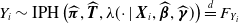 $Y_i\sim \text{IPH}\left(\widehat{\boldsymbol{\pi}}, \widehat{{\boldsymbol{T}}}, \lambda(\cdot \mid {\boldsymbol{X}}_i, \widehat{\boldsymbol{\beta}},\widehat{\boldsymbol{\gamma}})\right) \stackrel{d}{=} F_{Y_i}$
. As mentioned earlier, virtual lapses that happen after the contract maturity are a simple construction of our methodology. It suffices to consider
$Y_i\sim \text{IPH}\left(\widehat{\boldsymbol{\pi}}, \widehat{{\boldsymbol{T}}}, \lambda(\cdot \mid {\boldsymbol{X}}_i, \widehat{\boldsymbol{\beta}},\widehat{\boldsymbol{\gamma}})\right) \stackrel{d}{=} F_{Y_i}$
. As mentioned earlier, virtual lapses that happen after the contract maturity are a simple construction of our methodology. It suffices to consider
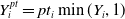 $Y_{i}^{pt} = pt_i\min(Y_i,1)$
instead, where
$Y_{i}^{pt} = pt_i\min(Y_i,1)$
instead, where
 $pt_i$
denotes the policy term in years (or any other time unit). We have
$pt_i$
denotes the policy term in years (or any other time unit). We have
 \begin{equation} {\mathbb P}\left(Y_{i}^{pt}\le t \right) = \left\{\begin{array}{cc} F_{Y_i}\left(\frac{t}{pt_i}\right), & 0 \le t \le pt_i \\ 1, & t \gt pt_i \end{array}\right.\end{equation}
as the distribution of the effective time until a lapse occurs. Note that the time unit corresponds to the one from
 $pt_i$
, which is years in our case.
$pt_i$
, which is years in our case.
As (5.1) is readily available, we can easily extract the distribution of the remaining contract lifetime before a lapse occurs. Let
 $T_{i,y}$
denote the remaining lifetime of contract i, given that y years have passed since the issuance of the policy. Its distribution is given by
$T_{i,y}$
denote the remaining lifetime of contract i, given that y years have passed since the issuance of the policy. Its distribution is given by
 \begin{equation} {}_{t}{p^{i}}_{y} = {\mathbb P}\left(T_{i,y} \ge t \right) = \frac{{\mathbb P}\left( Y_{i}^{pt}\ge y+t\right)}{{\mathbb P}\left(Y_{i}^{pt}\ge y \right)} =\left\{ \begin{array}{cc} \frac{1-F_{Y_i}\left(\frac{y+t}{pt_i}\right)}{1-F_{Y_i}\left(\frac{y}{pt_i}\right)}, & y+t\le pt_i \\ 0, & y+t\gt pt_i \end{array}\right. \quad.\end{equation}
This conditional survival perspective aligns with some of the standard actuarial frameworks used in pricing life insurance products and annuities. By using these methods, we can incorporate survival dynamics into surrender value pricing and liquidity risk assessment, as the survivorship component needed to discount future monetary flows is fully determined by (5.2). If information on surrender values is known, our methodology allows us to calculate the actuarial present value (APV) of cash flows caused by policyholder lapsing. For example, if a unitary surrender value is paid at the time of lapse and a constant interest rate is assumed, the APV would be
 \begin{equation}A^{i}_x = \int_0^{pt_i} v^s \, {}_s p^i_x \, \mu^i_{x+s} \, ds.\end{equation}
Here, v is the discount factor and
 $\mu^i_{x}$
is the force of mortality for a policy “aged” x. Once all parameters needed by the PI model are available, any actuarial calculation relying on a lifetime distribution can be readily employed, allowing for a practical use of such a framework.
$\mu^i_{x}$
is the force of mortality for a policy “aged” x. Once all parameters needed by the PI model are available, any actuarial calculation relying on a lifetime distribution can be readily employed, allowing for a practical use of such a framework.
6. Conclusion
In this paper, we investigated the determinants of lapse in credit life insurance contracts. Using real data from the French credit life insurance market, we employ the proportional intensities framework based on inhomogeneous phase-type distributions. Such a framework provides a flexible yet parsimonious survival model that captures the influence of policyholder characteristics, policy features, and macroeconomic factors on contract lifetimes. Methodologically, we extend the PI–IPH estimation framework to right-censored credit life data with shrinkage and show that the approach is feasible at portfolio scale.
Our findings show the importance of economic conditions, particularly of relative interest rate and inflation fluctuations, in shaping lapse behavior. Additionally, key policyholder attributes, such as age and loan type, were found to greatly influence contract survival probabilities. Our empirical evidence shows that lapse behavior is mainly governed by the interaction between macro-financial pressures on the policyholder and the residual liability of the loan. Contracts with a large outstanding sum insured are more prone to early termination, and this sensitivity is increased in periods of elevated inflation or when market rates rise above the contractual loan rate. Rather than a single cause, we observe that an interplay between the interest rate and emergency fund hypotheses motivates lapses.
The proposed PI model offers an interpretable framework, allowing us to assess not just the expected lapse rates but the full conditional distribution of policyholder contract durations. Thus, the estimated distributions can be exploited for stress-testing exercises, Solvency-II lapse-risk calibrations and product-pricing frameworks without sacrificing interpretability.
Additionally, the present work can be used to assess the quality of any profitability-related projections affected by lapsing. Our framework converts statistical insights into a tangible tool for insurers. Given the full conditional distribution of contract lifetimes until lapse, actuaries can set premiums and margins that reflect the “actual” timing of surrender/lapse risk. Moreover, these distributions can be integrated into forward cash flow and other actuarial estimates regarding this kind of products, reducing the gap between projected and realized profit.
Several limitations should be acknowledged. First, the empirical application is confined to a single French insurer, so structural differences across providers or business lines lie outside the scope of our study. Depending on the financing covered by a policy, the effect of macroeconomic variables can vary significantly. Nonetheless, our modeling framework can be employed on a portfolio basis, without worrying about such aspects.
Second, our decision to reduce time-varying covariates into relative indicators, rather than modeling their full historical changes, could hinder interpretability. On top of simplicity, it is attractive to work with covariates that are readily available at the time of issuance of the policy. Indeed, the history of market interest rates (for example) would not be available for a new contract. In our framework, all the relative growth rates would simply be disregarded. They would not impact the intensity function, nor the proportionality term, as their growth rate would be null.
Third, we do not provide a full predictive backtesting study or bootstrap-based uncertainty estimates for coefficients. Each model fit on the full portfolio is computationally intensive (about one week on a dedicated virtual machine), and resampling or repeated train/test splits would multiply this cost. Our focus here is on distributional interpretation rather than prediction; systematic validation and variance estimation are therefore left to future work as computing resources allow.
Lastly, in our application, the shrinkage term seems not to be needed. Nonetheless, such a modeling feature becomes very attractive when dealing with a large number of predictors. It is particularly useful in smaller samples or noisier settings where many covariates carry weak signals, and it provides a principled alternative to manual variable screening. That is, the shrinkage component of the model can replace expert judgment, or at least reduce its importance.
Future research could explore alternative functional forms for the inhomogeneous intensities, as well as incorporate additional explanatory variables to improve model accuracy. Additionally, expanding the PI regression framework would improve the interpretability of the results. Similarly to generalized additive models (see Hastie and Tibshirani Reference Hastie and Tibshirani1986), functional predictors could be modeled exploiting basis function expansions. This way, the model would be capable of dealing with time-dependent covariates and would provide an additional degree of interpretability.
In sum, our findings demonstrate that a carefully specified PI framework offers insurers a practical and theoretically grounded tool for anticipating and managing lapse risk in an ever-evolving economic landscape.
Acknowledgements
We are grateful to Swiss Re (L&H France) for providing the anonymized portfolio data that made this study possible. In particular, we thank Christophe Heck, Floriane Pian, and Quentin Vidal for their insightful discussions and constructive feedback throughout the development of this project.
Data availability statement
The dataset used in the paper is proprietary data from Swiss Re (L&H France) that we are unable to share.
Competing interests
The authors declare no conflict of interest or competing interests in this manuscript.
Appendix A. Estimation in case of interval-censoring
We present a generalization of Algorithm 1 in the case of interval-censored data. The main difference from before is that
 $Z\in(v,w)$
instead of
$Z\in(v,w)$
instead of
 $Z\in (v, \infty)$
. Moreover, we redefine the product set
$Z\in (v, \infty)$
. Moreover, we redefine the product set
 $\mathcal{Z}=\mathcal{Z}({\boldsymbol{z}})=\prod_{i=1}^N A_i$
, where
$\mathcal{Z}=\mathcal{Z}({\boldsymbol{z}})=\prod_{i=1}^N A_i$
, where
 $A_i=\{z_i\}$
if
$A_i=\{z_i\}$
if
 $\delta_i=1$
, and
$\delta_i=1$
, and
 $A_i=(z_i,w_i)$
otherwise. Then, it can be shown that the conditional expectations can be written as follows:
$A_i=(z_i,w_i)$
otherwise. Then, it can be shown that the conditional expectations can be written as follows:
-
(1) E-step, conditional expectations:
\begin{align*} &\mathbb{E}(B_k\mid {\boldsymbol{Z}}\in\mathcal{Z})=\sum_{i=1}^{N}\left\{ \delta_i\frac{\pi_k {{\boldsymbol{e}}_k}^{ \mathsf{T}}\exp( {\boldsymbol{T}} z_i) {\boldsymbol{t}} }{ \boldsymbol{\pi} \exp( {\boldsymbol{T}} z_i) {\boldsymbol{t}} }+(1-\delta_i)\frac{ \pi_{k} \left({\boldsymbol{e}}_{k}^{\mathsf{T}} \exp\left({\boldsymbol{T}} z_i\right){\boldsymbol{e}}-{\boldsymbol{e}}_{k}^{\mathsf{T}} \exp\left({\boldsymbol{T}} w_i\right){\boldsymbol{e}}\right) } { \boldsymbol{\pi} \exp\left({\boldsymbol{T}} z_i\right){\boldsymbol{e}}-\boldsymbol{\pi} \exp\left({\boldsymbol{T}} w_i\right){\boldsymbol{e}}}\right\},\end{align*}
\begin{align*} &\mathbb{E}(V_k\mid {\boldsymbol{Z}}\in\mathcal{Z})=\sum_{i=1}^{N} \left\{\delta_i\frac{\int_{0}^{z_i}{{\boldsymbol{e}}_k}^{ \mathsf{T}}\exp( {\boldsymbol{T}} (z_i-u)) {\boldsymbol{t}} \boldsymbol{\pi} \exp( {\boldsymbol{T}} u){\boldsymbol{e}}_kdu}{ \boldsymbol{\pi} \exp( {\boldsymbol{T}} z_i) {\boldsymbol{t}} } \right.\\ & \quad + (1-\delta_i)\left[\frac{\int_{z_i}^{w_i}{\boldsymbol{\pi}_k}\exp( {\boldsymbol{T}} u)du}{ \boldsymbol{\pi} \exp\left({\boldsymbol{T}} z_i\right){\boldsymbol{e}}-\boldsymbol{\pi} \exp\left({\boldsymbol{T}} w_i\right){\boldsymbol{e}}}\right. \\ & \quad + \left. \left.\frac{\int_{0}^{z_i}{{\boldsymbol{e}}_k}^{\mathsf{T}}\exp( {\boldsymbol{T}} (z_i-u)) {\boldsymbol{e}} \, \boldsymbol{\pi} \exp( {\boldsymbol{T}} u){\boldsymbol{e}}_kdu -\int_{0}^{w_i}{{\boldsymbol{e}}_k}^{\mathsf{T}}\exp( {\boldsymbol{T}} (w_i-u)) {\boldsymbol{e}} \, \boldsymbol{\pi} \exp( {\boldsymbol{T}} u){\boldsymbol{e}}_kdu}{ \boldsymbol{\pi} \exp\left({\boldsymbol{T}} z_i\right){\boldsymbol{e}}-\boldsymbol{\pi} \exp\left({\boldsymbol{T}} w_i\right){\boldsymbol{e}}}\right] \right\},\end{align*}


 \begin{align*}&\mathbb{E}(N_{kl}\mid{\boldsymbol{Z}}\in\mathcal{Z})=\sum_{i=1}^{N}t_{kl} \left\{\delta_i \frac{\int_{0}^{z_i}{{\boldsymbol{e}}_l}^{\mathsf{T}}\exp( {\boldsymbol{T}} (z_i-u)) {\boldsymbol{t}} \, \boldsymbol{\pi} \exp( {\boldsymbol{T}} u){\boldsymbol{e}}_kdu}{ \boldsymbol{\pi} \exp( {\boldsymbol{T}} z_i) {\boldsymbol{t}} } \right.\\&\quad\quad + (1-\delta_i)\left[\frac{\int_{z_i}^{w_i}{\boldsymbol{\pi}_k}\exp( {\boldsymbol{T}} u)du}{ \boldsymbol{\pi} \exp\left({\boldsymbol{T}} z_i\right){\boldsymbol{e}}-\boldsymbol{\pi} \exp\left({\boldsymbol{T}} w_i\right){\boldsymbol{e}}}\right. \\ & \quad + \left. \left.\frac{\int_{0}^{z_i}{{\boldsymbol{e}}_l}^{\mathsf{T}}\exp( {\boldsymbol{T}} (z_i-u)) {\boldsymbol{e}} \, \boldsymbol{\pi} \exp( {\boldsymbol{T}} u){\boldsymbol{e}}_kdu-\int_{0}^{w_i}{{\boldsymbol{e}}_l}^{\mathsf{T}}\exp( {\boldsymbol{T}} (w_i-u)) {\boldsymbol{e}} \, \boldsymbol{\pi} \exp( {\boldsymbol{T}} u){\boldsymbol{e}}_kdu}{ \boldsymbol{\pi} \exp\left({\boldsymbol{T}} z_i\right){\boldsymbol{e}}-\boldsymbol{\pi} \exp\left({\boldsymbol{T}} w_i\right){\boldsymbol{e}}}\right] \right\},\end{align*}
 \begin{align*}&\mathbb{E}(N_k\mid {\boldsymbol{Z}}\in\mathcal{Z})=\sum_{i=1}^{N} t_k\left\{\delta_i\frac{ \boldsymbol{\pi} \exp( {\boldsymbol{T}} z_i){{\boldsymbol{e}}}_k}{ \boldsymbol{\pi} \exp( {\boldsymbol{T}} z_i) {\boldsymbol{t}} }+(1-\delta_i)\frac{\int_{z_i}^{w_i}{\boldsymbol{\pi}_k}\exp( {\boldsymbol{T}} u)du}{ \boldsymbol{\pi} \exp\left({\boldsymbol{T}} z_i\right){\boldsymbol{e}}-\boldsymbol{\pi} \exp\left({\boldsymbol{T}} w_i\right){\boldsymbol{e}}}\right\}.\end{align*}
Note that the maximization step remains unchanged.
For convenience, a summary of the entire procedure is provided in Algorithm 2.
Full EM algorithm for the PI model, when data are interval-censored

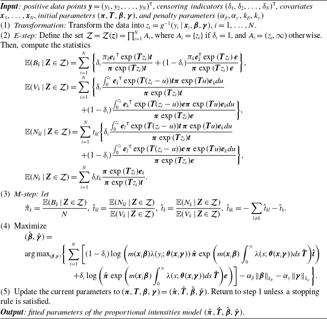
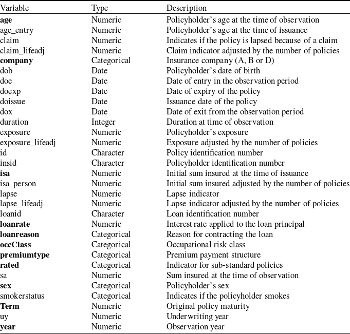
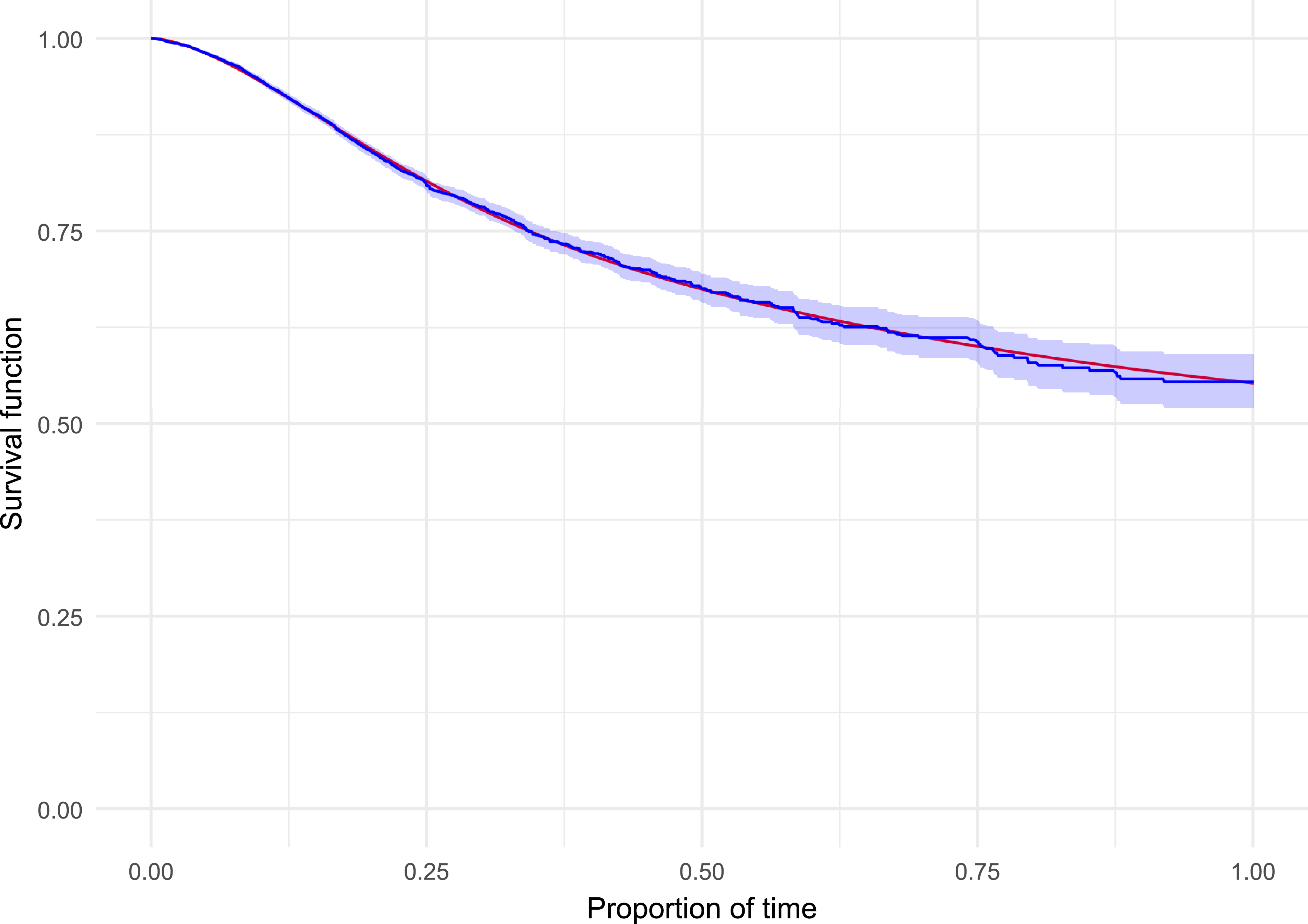
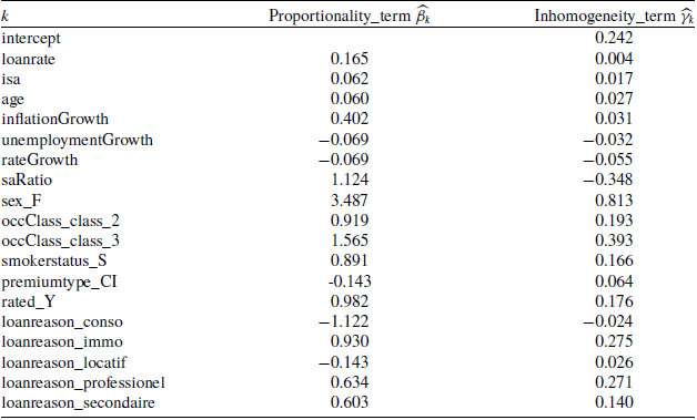
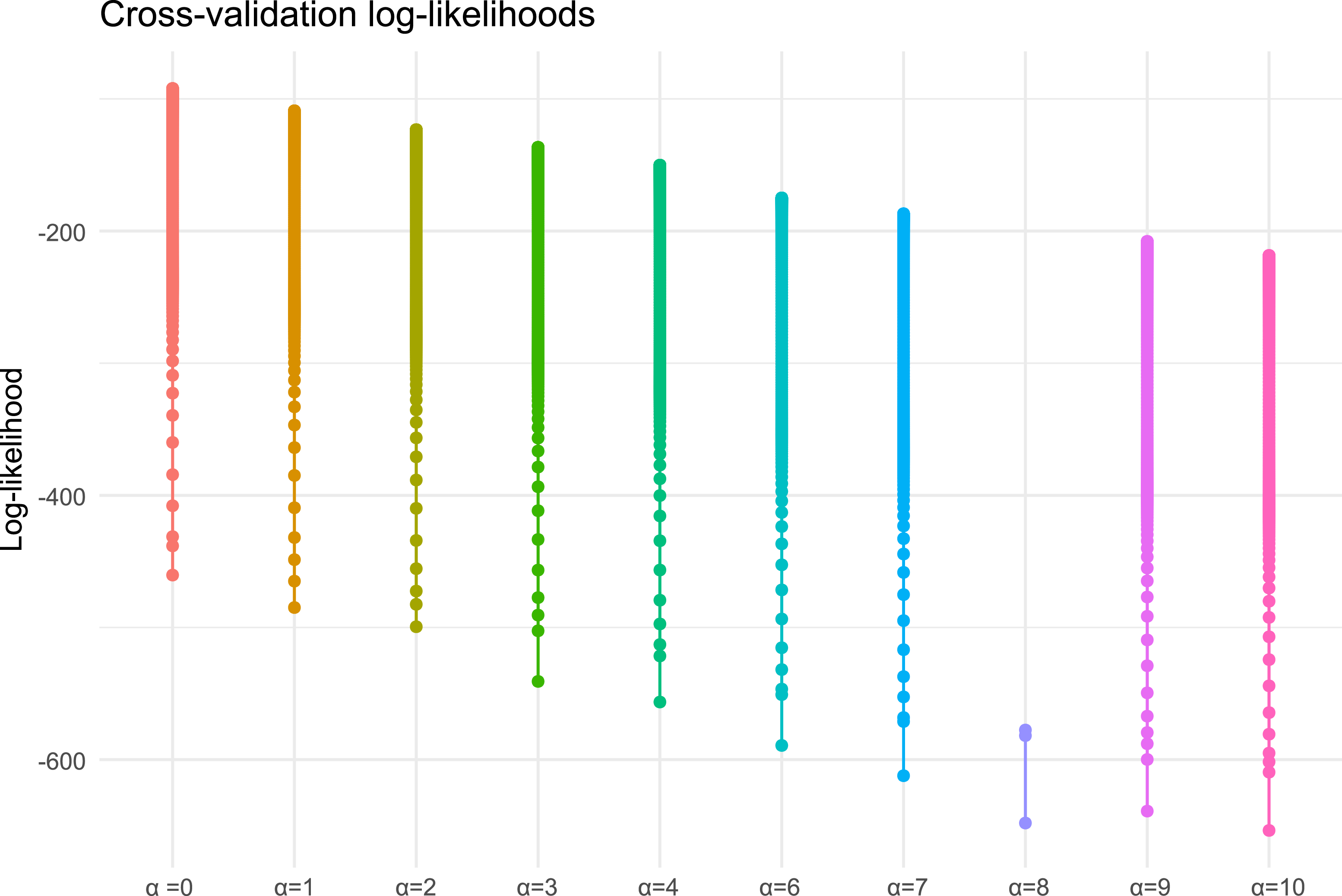


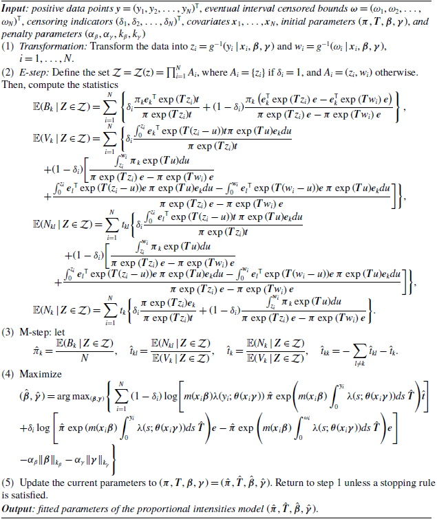

 Open access