2 Compositional outcomes and synthetic control methods

2.2 Pitfalls of separate estimation: An illustration

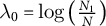
Before discussing estimators in abstract terms, we present a deliberately simplified hypothetical example to illustrate why separate estimation of compositional outcomes can yield logically incompatible treatment effects and thus motivates the search for a joint approach. Consider three countries A, B and C, where country A is affected by a treatment at time T, while countries B and C were not treated and constitute the donor pool for creating synthetic controls for outcomes of interest. Suppose that we are interested in the treatment effects on party vote shares in country A, and all the voters in each country choose among three party families: X (e.g., left), Y (e.g., center-right) and Z (e.g., far right). Thus, the synthetic controls for the vote shares of each party in country A are obtained by weighting the vote shares of the same party family in countries B and C.

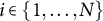
In the approach to synthetic controls currently prevalent in political science, one would apply the method to each outcome variable separately (e.g., Cremaschi et al. Reference Cremaschi, Rettl, Cappelluti and Vries2024), often focusing on one party of interest (e.g., Becher et al. Reference Becher, González and Stegmueller2023; Hilbig and Riaz Reference Hilbig and Riaz2024). Following a synthetic approach with intercept shifts, in our example, a researcher interested in the treatment effects would create a synthetic control for each party X, Y and Z separately, trying to approximate that party’s pre-treatment trend in A by congenial party trends in B and C. For example, if A’s pre-treatment trend is a bisector between the trends in B and C, then the optimal synthetic control for A comprises B and C half-and-half (Figure 1, left). However, this does not mean that synthetic controls for the vote shares of Y and Z assign the same weights to countries B and C. For the vote share of party family Y, the synthetic control for country A is constructed entirely from country B, while for party family Z, it is constructed entirely from country C (Figure 1, center and right). As a result, the estimated treatment effect in country A is zero for parties X and Y, but positive for Z. This discrepancy arises even though the true vote shares across X, Y and Z necessarily sum to one (100%) in every country and period.

Figure 1

Illustrative example of inconsistencies in synthetic control weights across proportional outcomes (party vote shares).

Thus, using SCMs on each party X, Y and Z separately can lead to effect estimates that do not sum to zero because each estimate is essentially obtained using a different control. In practice, different comparisons across outcomes can yield conflicting findings for elements of the same whole. This incompatibility may not be apparent when analyzing a single party, but it becomes observable when effects are estimated across multiple parties (or when abstention is regarded as a part in the composition), as recommended by the literature on compositional outcomes and electoral effects (Cohen, Krause, and Abou-Chadi Reference Cohen, Krause and Abou-Chadi2024; Katz and King Reference Katz and King1999; Lipsmeyer et al. Reference Lipsmeyer, Philips, Rutherford and Whitten2019; Philips, Rutherford, and Whitten Reference Philips, Rutherford and Whitten2015, Reference Philips, Rutherford and Whitten2016).

In what follows, we formally discuss how a joint synthetic control estimation for multiple outcomes addresses this pitfall (Sections 3 and 4) and evaluate its performance in simulation (Section 5) and empirical implications (Section 6).

3 Constant control comparison

To analyze causal effects on compositional data, we formally introduce the constant control comparison, a sufficient condition that ensures treatment effect estimates satisfy the sum constraint. We focus on a balanced panel with N units at T time points. For each unit $i \in \{1, \ldots , N\}$ , treatment status is indicated by $D_i \in \{0,1\}$ . We observe $N_{tr}$ treated ( $D_i = 1$ ) and $N_{co}$ untreated control units ( $D_i = 0$ ). For notational simplicity, we arrange the unit indices i so that all treated units follow all untreated units $i\in \{1,\ldots , N_{co},N_{co}+1, \ldots ,N\}$ . In this section, we consider the case where exposure to treatment occurs in the last period $T = T_{0} + 1$ , but the notation and results generalize to multiple post-treatment periods.

The compositional outcomes of interest $y_{itk}$ form a vector $(y_{it1},\ldots ,y_{itK})$ of length K for each unit $i \in \{1,\ldots ,N\}$ and time point $t \in \{1,\ldots ,T\}$ . For the post-treatment period, we introduce potential outcomes under the control condition $y_{iTk}(0)$ and under the treatment condition $y_{iTk}(1)$ . We focus on estimating the average treatment effects on the treated (ATT) for each compositional outcome: $\tau _k = \mathbb {E}[y_{iTk}(1) \mid D_{i} = 1] - \mathbb {E}[y_{iTk}(0) \mid D_{i} = 1]$ . Since the outcomes for the treated units under treatment are observable, $\mathbb {E}[y_{iTk}(1) \mid D_{i} = 1]$ can be estimated from the data in a consistent and unbiased way as $ \frac {1}{N_{tr}} \sum _{i=N_{co} +1}^N y_{iTk}$ . However, the counterfactual $\mathbb {E}[y_{iTk}(0)\mid D_i=1]$ must be estimated from control outcomes. To do this, SCMs calculate a set of non-negative weights $\hat {\omega }_{ik}$ that align the control outcomes with the pre-exposure trajectory of the treated units. This weighting principle underlies the classic SCM (Abadie et al. Reference Abadie, Diamond and Hainmueller2010, Reference Abadie, Diamond and Hainmueller2015), where weights are chosen so that $\sum _{i=1}^{N_{co}} \hat {\omega }_{ik} y_{itk} \approx \frac {1}{N_{tr}} \sum _{i=N_{co}+1}^{N} y_{itk}$ for all $~ t \in \{1, \ldots , T_0\}$ and for all $k \in \{1, \ldots , K\}$ . Its extensions with intercept shifts (Ferman and Pinto Reference Ferman and Pinto2021) and the SDID method (Arkhangelsky et al. Reference Arkhangelsky, Athey, Hirshberg, Imbens and Wager2021) further include additive unit-level shifts and time weights $\hat {\lambda }_{tk}$ , as formally described in Section 1 of the Supplementary Material.

By definition of compositional data, all K proportions $y_{itk}(d)$ are bound between 0 and 1 and sum to 1 for all observations i, time points t and the two treatment states $d \in \{0,1\}$ . Thus, under the compositional constraint, the sum of average treatment effects on the separate proportions should be zero.

Lemma 1 Constraint on ATTs for proportions

For compositional data where $0 \leq y_{itk}(d) \leq 1~\forall ~k$ and $\sum _{k=1}^K y_{itk}(d) = 1$ , it holds that

(1) $$ \begin{align} \sum_{k=1}^K {\tau}_k = \sum_{k=1}^K \mathbb{E}[y_{iTk}(1) - y_{iTk}(0) \mid D_{i} = 1] = 0, \end{align} $$

where $y_{itk}(d)$ is the potential outcome under treatment status $d \in \{0,1\}$ .

It holds by linearity of expectation: the sum of the treatment effects equals the expected difference between the total proportion under treatment and under control, and since both totals are constrained to equal one, the expectation is zero (see also Section 2 of the Supplementary Material). Lemma 1 implies that if one proportion increases under treatment exposure, another has to decrease, leading to a sum constraint over the treatment effects of zero. Violations of the constraint on the ATTs lead to contradictory interpretations of the effects on different proportions and can make it difficult to interpret the results.

To see whether synthetic control estimators satisfy Lemma 1, we integrate compositional outcomes with the SDID framework (Arkhangelsky et al. Reference Arkhangelsky, Athey, Hirshberg, Imbens and Wager2021). SDID generalizes over both DID and a range of SCMs, both with and without additive unit-level shifts and/or time weights. Section 1 of the Supplementary Material formally describes the method following Arkhangelsky et al. (Reference Arkhangelsky, Athey, Hirshberg, Imbens and Wager2021). The SDID estimator for proportion k can be written as a weighted double difference.

Definition 1 SDID estimator

(2) $$ \begin{align} \begin{aligned} \widehat{\tau}_k^{\mathrm{sdid}} &= \underbrace{ \left( \frac{1}{N_{\mathrm{tr}}} \sum_{i=N_{\mathrm{co}}+1}^{N} y_{iTk} - \sum_{j=1}^{N_{\mathrm{co}}} \omega_{jk} \, y_{jTk} \right) }_{\text{post-treatment: treated vs. weighted control}} \\ &\quad - \underbrace{ \left( \frac{1}{N_{\mathrm{tr}}} \sum_{i=N_{\mathrm{co}}+1}^{N} \sum_{t=1}^{T_0} \lambda_{tk} \, y_{itk} - \sum_{j=1}^{N_{\mathrm{co}}} \omega_{jk} \sum_{t=1}^{T_0} \lambda_{tk} \, y_{jtk} \right) }_{\text{time-weighted pre-treatment: treated vs. weighted control}} \; , \end{aligned} \end{align} $$

where $\omega _{jk}$ are of non-negative unit weights that sum to one: $\sum _{j=1}^{N_{co}} \omega _{jk} = 1$ and $\lambda _{tk}$ are non-negative time weights that sum to one: $\sum _{t=1}^{T_0} \lambda _{tk} = 1$ for all k.

In case of compositional data, cross-outcome weight invariance is crucial to whether the ATT sum constraint holds. For standard DID, all weights are the same across outcomes by construction: $\forall ~k \in \{1,\ldots , K\}$ , unit weights $\omega _{jk} = 1/N_{co}$ and time weights $\lambda _{tk} = 1/T_0$ . However, SCMs choose unit weights to fit the pre-treatment outcomes, as formally discussed in Section 1 of the Supplementary Material. Separate applications of SCMs to proportions can yield weights that can differ across outcomes for the same unit: there exist $ k, k' \in \{1, \ldots , K\}$ with $k \neq k'$ such that $\omega _{ik} \neq \omega _{ik'}$ .

In contrast, we define the constant control comparison for compositional data in the following way.

The constant control comparison enables the use of the same weights for all proportional outcomes of a unit. We denote them by $\omega _j$ and $\lambda _{t}$ in the SDID estimator, rather than outcome-specific $\omega _{jk}$ and $\lambda _{tk}$ . These common weights across outcomes are a sufficient (though not necessary) condition that the constraint on ATTs for proportional outcomes is met.

Theorem 1 Sufficiency of constant control comparison

Under constant control comparison (see Definition 2), the SDID estimates of the ATT (see Definition 1) satisfy the constraint on the ATTs for proportions (see Lemma 1), that is, sum to zero:

(3) $$ \begin{align} \begin{aligned} \sum_{k=1}^K \hat{\tau}_k &= { \big[ \underbrace{\frac{1}{N_{\mathrm{tr}}}\sum_{i=N_{\mathrm{co}}+1}^{N} \sum_{k=1}^K y_{iTk}}_{=1}\ -\ \underbrace{\sum_{j=1}^{N_{\mathrm{co}}} \omega_j \sum_{k=1}^K y_{jTk}}_{=\sum_j \omega_j \cdot 1=1}\big]\ }\\ &\quad { -\ \big[ \underbrace{\frac{1}{N_{\mathrm{tr}}}\sum_{i=N_{\mathrm{co}}+1}^{N}\sum_{t=1}^{T_0}\lambda_t \sum_{k=1}^K y_{itk}}_{=\sum_t \lambda_t \cdot 1=1}\ -\ \underbrace{\sum_{j=1}^{N_{\mathrm{co}}} \omega_j \sum_{t=1}^{T_0}\lambda_t \sum_{k=1}^K y_{jtk}}_{=\sum_j \omega_j \sum_t \lambda_t \cdot 1=1}\big]} = 0. \end{aligned} \end{align} $$

If the constant control comparison is violated, the sum-to-zero constraint on the ATTs for proportions does not necessarily hold (see Section 2 of the Supplementary Material for an illustrative counterexample with weights that differ across outcomes). The same logic extends to the demeaned weighting estimator of Doudchenko and Imbens (Reference Doudchenko and Imbens2016), ass shown in Section 3 of the Supplementary Material. In the context of SCMs, re-estimating weights separately for each outcome can therefore violate the constraint. To satisfy the constraint on the ATTs for compositional data, we propose using common weights for all proportions to ensure a constant control comparison.Footnote ⁵

4 Implementing common weights in synthetic difference-in-differences

Based on the insights from Section 3, we formulate an SDID approach that follows the constant control comparison. In contrast to the original method (Arkhangelsky et al. Reference Arkhangelsky, Athey, Hirshberg, Imbens and Wager2021), we reconfigure the minimization problem to obtain the same set of unit and time weights across outcomes. While common weights have been previously introduced for synthetic controls, with one treated unit (Sun et al. Reference Sun, Ben-Michael and Feller2025; Tian et al. Reference Tian, Lee and Panchenko2023), we adopt them for SDID.

Our approach to SCMs for compositional data imposes the same set of unit weights for all proportional outcomes $\hat {\omega }_{i}$ and does the same for time weights $\hat {\lambda }_{t}$ in the case of synthetic DID. The control unit weights ${\omega }^{\mathrm {co}} = ({\omega }_0,{\omega }_1,\ldots ,{\omega }_{N_{co}})$ are obtained by minimizing the squared deviations of the weighted control outcomes from the average treated outcomes across all proportions:

(4) $$ \begin{align} \hat{\omega}^{\mathrm{co}} & = \underset{{\omega}^{\mathrm{co}} \in \Omega}{\mathop{\mathrm{arg\,min}}} ~ \ell_{unit}({\omega}^{\mathrm{co}}) , ~ \text{where} \\ \nonumber & \ell_{unit}({\omega}^{\mathrm{co}}) = \sum_{k=1}^{K} \Bigg ( \sum_{t=1}^{T_0} \left( {\omega}_{0} + \sum_{i=1}^{N_{co}} {\omega}_{i} y_{itk} - \frac{1}{N_{tr}} \sum_{i=N_{co}+1}^{N} y_{itk} \right)^2 \Bigg ) + \xi^2 T_0 \sum_{i=1}^{N_{co}} \omega_{i}^2, \\ \nonumber & \Omega = \Bigg \{{\omega}^{\mathrm{co}} : \omega_{0} \in \mathbb{R}, ~\omega_{i} \in \mathbb{R}_{+} ~\forall ~ i \in \{1, \ldots, N_{co}\}, ~\sum_{i=1}^{N_{co}} \omega_i = 1 \Bigg \}. \end{align} $$

The same set of weights is chosen to optimize the pre-treatment fit jointly over all $T_0$ pre-treatment periods and K outcomes. The objective function in problem (4) further includes a regularization parameter $\xi $ , which penalizes extreme weights using a squared $L_2$ norm of the weight vector.Footnote ⁶ Controlling the dispersion this way facilitates the uniqueness and stability of the solution, leading to more robust estimations (see also Doudchenko and Imbens Reference Doudchenko and Imbens2016). Combining the control-unit weights $\hat {\omega }^{\mathrm {co}}$ with uniform weights ${1}/{N_{tr}}$ for treated units yields the full-sample unit weights:

(5) $$ \begin{align} \hat{\omega}_i = \begin{cases} \hat{\omega}^{\mathrm{co}}_i, & i=1,\ldots,N_{co},\\ \frac{1}{N_{tr}}, & i=N_{co}+1,\ldots,N. \end{cases} \end{align} $$

As in the case of unit weights, we compute pre-treatment time weights $\lambda ^{\mathrm {pre}}=(\lambda _0,\lambda _1,\ldots ,\lambda _{T_0})$ jointly for all K outcomes by solving:

(6) $$ \begin{align} \hat{\lambda}^{\mathrm{pre}} & = \underset{\lambda^{\mathrm{pre}} \in \Lambda}{\mathop{\mathrm{arg\,min}}} ~ \ell_{time}({\lambda}^{\mathrm{pre}}) , ~ \text{where} \\ \nonumber & \ell_{time}({\lambda}^{\mathrm{pre}}) = \sum_{k=1}^K \Bigg ( \sum_{i=1}^{N_{co}} \left( {\lambda}_{0} + \sum_{t=1}^{T_0} {\lambda}_{t} y_{itk} - \frac{1}{T-T_0} \sum_{t=T_0+1}^{T} y_{itk} \right)^2 \Bigg ), \\ \nonumber & \Lambda = \Bigg \{ \lambda^{\mathrm{pre}} :\ \lambda_{0}\in\mathbb{R},\ \lambda_{t}\in\mathbb{R}_{+}\ \forall\, t\in\{1,\ldots,T_0\},\ \sum_{t=1}^{T_0} \lambda_t = 1 \Bigg \}. \end{align} $$

Together, the pre-treatment weights and the uniform post-treatment weights form the full period time weights:

(7) $$ \begin{align} \hat\lambda_t = \begin{cases} \hat{\lambda}^{\mathrm{pre}}_t, & t=1,\ldots,T_0,\\ \frac{1}{T-T_0}, & t=T_0+1,\ldots,T. \end{cases} \end{align} $$

Using both $\hat {\omega }_i$ from Equation (5) and $\hat \lambda _t$ from Equation (7), we now obtain the SDID estimates for each outcome k from the following two-way fixed effects regression:

(8) $$ \begin{align} (\hat{\tau}_k^{sdid},\hat{\mu}_{k}, \hat{\alpha}_{ik},\hat{\beta}_{tk}) = \underset{\tau,\mu, \alpha,\beta}{\mathrm{arg\,min}} \Bigg \{ \sum_{i=1}^N \sum_{t=1}^T \left( y_{itk} - \mu_k - \alpha_{ik} - \beta_{tk} - D_{it} \tau \right)^2 \hat{\omega}_i \hat{\lambda}_t \Bigg \}, \end{align} $$

where $\alpha _{ik}$ are unit fixed effects and $\beta _{tk}$ are time fixed effects for each outcome.

Algorithm 1 summarizes the overall procedure for the SDID estimator with common weights. We first calculate the regularization parameter and then compute the unit weights followed by the time weights. Afterward, we obtain the treatment effect estimates using the weighted two-way regression for each proportion.

Alternatively, a similar procedure can be used to estimate classic SCM models, usually applied in contexts with one treatment unit (Abadie et al. Reference Abadie, Diamond and Hainmueller2010, Reference Abadie, Diamond and Hainmueller2015). For this algorithm, described in Section 4 of the Supplementary Material, we skip the time weight estimation, excluding the time weights from the regression model. We further exclude the constant in the calculation of the unit weights, which does not allow for an intercept shift in pre-treatment trends. For compositional proportional outcomes, we implement common weights for both the synthetic DID and the classic synthetic control in our R-package propsdid (Stoetzer and Bogatyrev Reference Stoetzer and Bogatyrev2026), which extends the synthdid package (Hirshberg Reference Hirshberg2022) to multivariate outcomes with constant control comparisons.

To estimate the uncertainty around our treatment effect estimates from SDID with common weights, we rely on the same approaches to variance estimation as in Arkhangelsky et al. (Reference Arkhangelsky, Athey, Hirshberg, Imbens and Wager2021): clustered bootstrap (Efron Reference Efron1979), jackknife methods (Miller Reference Miller1974) and placebo inference (Abadie et al. Reference Abadie, Diamond and Hainmueller2010). The latter is particularly valuable when there are very few treated units and involves applying placebo treatments to control units to estimate the level of noise, similar to the approach of Conley and Taber (Reference Conley and Taber2011). Each of these methods strikes a balance between computational complexity and robustness, depending on the structure of the dataset. For large panels, bootstrap is often favored for its reliability, whereas the jackknife and placebo methods provide useful alternatives when computational efficiency or small-sample concerns are more pressing. In our application, we rely on the jackknife method.

5 Simulation study

In this section, we evaluate the statistical performance of the synthetic control estimator with common weights for compositional outcomes. Estimation error in the classic SCM generally arises from two sources: approximation error, reflecting the donor pool’s inability to reproduce the treated unit’s counterfactual path, and estimation error, resulting from overfitting idiosyncratic noise in pre-treatment outcomes (Abadie et al. Reference Abadie, Diamond and Hainmueller2010). While regularization can mitigate overfitting, approximation bias can persist even as the number of pre-treatment periods increases (Ferman and Pinto Reference Ferman and Pinto2021).

Recent work suggests that aggregating information across multiple related outcomes can stabilize weight estimation. By fitting a common set of weights in the classic SCM under a shared latent factor structure, researchers can effectively average out idiosyncratic variation, yielding tighter finite-sample bias bounds than separate weights (Sun et al. Reference Sun, Ben-Michael and Feller2025; Tian et al. Reference Tian, Lee and Panchenko2023). Intuitively, this improves the signal-to-noise ratio in the pre-treatment matching objective.

These insights are relevant here, yet they do not directly map onto SDID with compositional outcomes. While Arkhangelsky et al. (Reference Arkhangelsky, Athey, Hirshberg, Imbens and Wager2021) establish consistency and asymptotic normality for univariate SDID, the estimator already incorporates unit and time weights that reduce variance. It is therefore an open question whether the gains from common weights scale in SDID as they do in classic synthetic control settings. Moreover, the simplex constraint implies a non-linear outcome space, which makes it analytically challenging to derive formal bias bounds using standard linear factor models.

We therefore rely on a comprehensive simulation study, calibrated to panel data structures commonly used in political science, to assess finite-sample performance, focusing on whether common weights preserve statistical efficiency while ensuring coherent interpretation of compositional treatment effects.

To define the data-generating process (DGP) for our simulation study, we use a dynamic latent-state model. The panel data consist of N units observed over T time periods, with outcomes given by K proportions that sum to one in each unit–time cell. A subset of $N_1$ units is exposed to treatment from period $T_1$ onward.Footnote ⁷ For each unit i and proportion k, outcomes are driven by two latent components: a level and a trend. The level captures persistent, unit-specific differences in baseline support for a given proportion, while the trend captures unit-specific trajectories over time. Both components are unit- and proportion-specific. 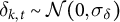At the start of the panel ( $t=0$ ), we draw initial latent states from normal distributions:

(9) $$ \begin{align} \gamma_{i,k,0} \sim \mathcal{N}(\mu_{\gamma_{k,0}}, \sigma_{\gamma_{k,0}}), \quad \upsilon_{i,k,0} \sim \mathcal{N}(\mu_{\upsilon_{k,0}}, \sigma_{\upsilon_{k,0}}), \end{align} $$

where $\gamma _{i,k,0}$ denotes the levels and $\upsilon _{i,k,0}$ denotes the trends. The hyperparameters ( $\mu _{\gamma _{k,0}},\mu _{\upsilon _{k,0}}$ ) control cross-unit heterogeneity at baseline. The trends are particularly useful for simulating violations of parallel trends assumption, since treated and control units may differ in their pre-treatment trajectories even if levels are similar. We therefore let treatment assignment depend on latent characteristics of one proportion j, by defining a weighted scalar index 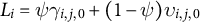$L_i = \psi \gamma _{i,j,0} + (1 - \psi )\upsilon _{i,j,0}$ which allows treatment selection to depend either on baseline levels ( $\psi = 1$ ) or trends ( $\psi = 0$ ). Units with higher values of $L_i$ are more likely to be treated, with assignment probabilities given by a logistic function: 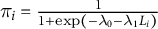$\pi _i = \frac {1}{1 + \exp (-\lambda _0 - \lambda _1 L_i)}$ , where $\lambda _0,\lambda _1$ are hyperparameter that sets the strength of treatment selection based on latent factors. Treatment is then assigned such that exactly $N_1$ units are treated.Footnote ⁸

Latent levels evolve over time according to autoregressive processes:

$$\begin{align*}\gamma_{i,k,t+1} = \rho_{\gamma_k}\gamma_{i,k,t} + \upsilon_{i,k,t} + \epsilon_{\gamma_{i,k,t}}, \quad \upsilon_{i,k,t+1} = \rho_{\upsilon_k}\upsilon_{i,k,t} + \epsilon_{\upsilon_{i,k,t}}, \end{align*}$$

with normally distributed shocks. These dynamics generate persistent unit-level heterogeneity and smoothly evolving trends.Footnote ⁹ For each unit, time and proportion, we construct a latent outcome

$$\begin{align*}\widetilde{Y}_{i,k,t} = \gamma_{i,k,t} + \tilde{\tau}_k W_{i,t} + \delta_{k,t} + \epsilon_{i,k,t}, \end{align*}$$

where $\tilde {\tau }_k$ denotes the latent treatment shift, $\delta _{k,t}$ denotes common time shocks that are drawn from a normal distribution $ \delta _{k,t} \sim \mathcal {N}(0, \sigma _{\delta }) $ and $\epsilon _{i,k,t}$ denotes idiosyncratic noise. Observed outcomes are obtained via a multinomial link:

$$\begin{align*}Y_{i,k,t} = \frac{\exp(\widetilde{Y}_{i,k,t})}{\sum_{k=1}^K \exp(\widetilde{Y}_{i,k,t})}, \end{align*}$$

which ensures that proportions are non-negative and sum to one. This DGP allows us to flexibly vary sample size, time horizon, treatment selection and the presence of level-differences or trends, while preserving the compositional structure of the outcomes.

Our simulation DGP differs from the static low-rank factor model commonly used to justify synthetic control and SDID estimators. Standard theoretical results assume that outcomes follow a factor structure of the form $\widetilde {Y}_{i,k,t} = \lambda _{i,k}' f_{t,k} + \varepsilon _{i,k,t}$ , where $\lambda _{i,k}$ denotes unit- and outcome-specific factor loadings, $f_{t,k}$ denotes outcome- and time-specific factors and $\varepsilon _{i,k,t}$ is an idiosyncratic error term (see, e.g., Ferman, Pinto, and Possebom Reference Ferman, Pinto and Possebom2020; Xu Reference Xu2017). In this formulation, the loadings are fixed over time and no explicit temporal structure is imposed on the factors, which are treated as unrestricted time-specific parameters. In contrast, we allow the latent factors to evolve autoregressively over time.

An autoregressive factor process can be written in companion form as a first-order linear state-space system by stacking lagged factors into an augmented state vector (see, e.g., Hamilton Reference Hamilton1994, 372–374). Consequently, dynamic factor models have an equivalent static representation in higher dimension. Our DGP therefore remains within the class of linear low-rank factor models underlying synthetic control estimators, while introducing structured temporal dependence that is not typically emphasized in the theoretical literature.Footnote ¹⁰ We adopt this dynamic specification because many proportional political outcomes, such as vote shares, exhibit substantial persistence and evolve gradually over time. The autoregressive structure thus reflects the empirical properties of these outcomes more closely than a static factor model.

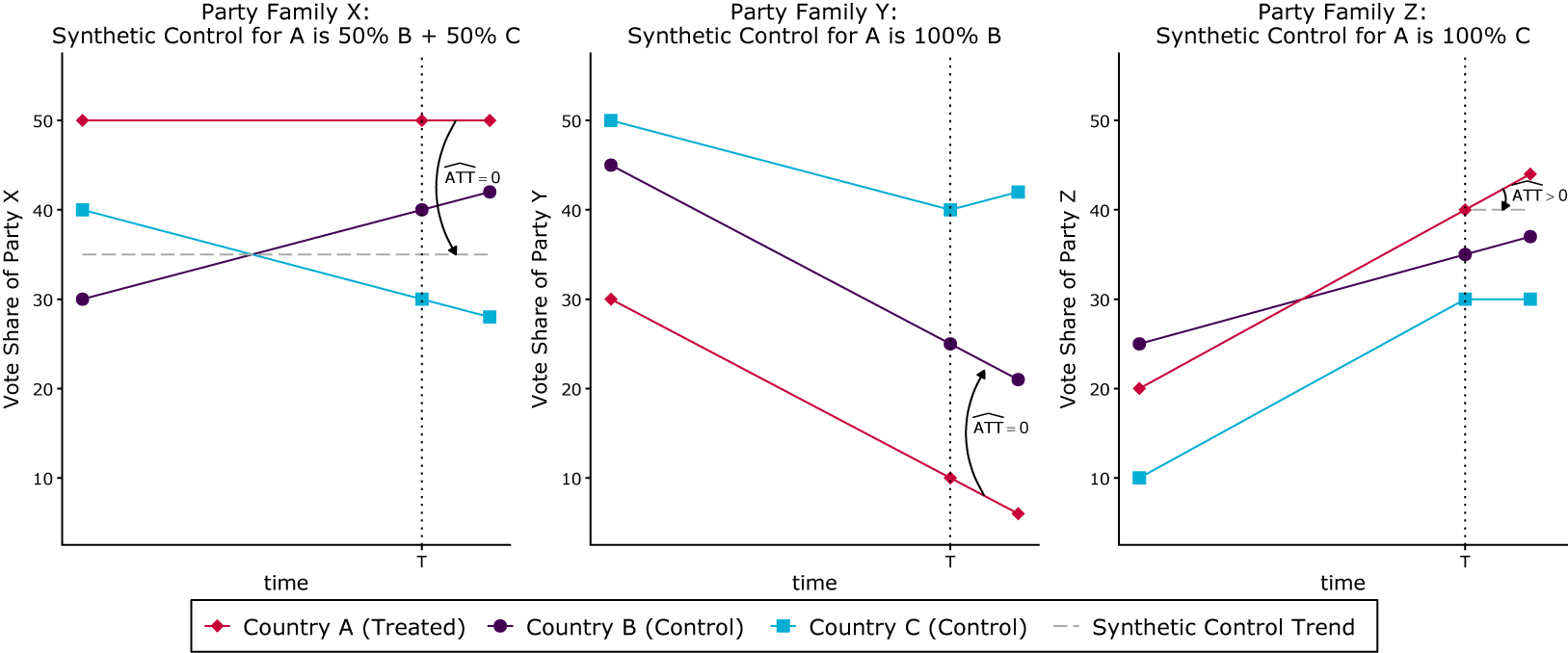
We analyze scenarios with four proportions and a latent treatment effect on the first proportion (for an example, see Section 5 of the Supplementary Material).Footnote ¹¹ The simulation scenarios contain 5 and 10 time points, where the treatment occurs either in the final period or in the last two periods. We consider 50, 200 and 1,000 units, with treatment proportions of 10% and 50%, and one and two treatment periods. The different scenarios reflect common data settings in applied work and vary the number of available pre-treatment control units, which is relevant for mitigating approximation error in the construction of counterfactual outcome trajectories. Treatment assignment is implemented in two ways: based either on levels or on trends. This allows us to evaluate performance under different selection mechanisms, including cases with clear violations of the parallel trends assumption, where synthetic methods are expected to perform particularly well compared to standard DID.Footnote ¹² We draw 1,000 independent samples for each of 48 combinations and estimate DID using two-way fixed effects, an SC and an SDID model separately for each outcome, as well as SC and SDID with common weights across proportional outcomes. We compare the estimates based on standard deviation, root-mean-square error (RMSE) and absolute-valued bias. We also calculate the absolute deviation of the sum of the treatment effect estimates on the separate proportions, which under the constant control comparisons should be zero.Footnote ¹³

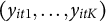
Table 1 reports results aggregated across all parameter settings, distinguishing between treatment selection based on levels and trends, with performance metrics averaged over all proportions. The table first highlights the importance of respecting the sum constraint when estimating treatment effects on proportional outcomes. Standard SCMs violate this constraint substantially, with average deviations of nearly 7 percentage points under both treatment selection designs. SDID also exhibits non-negligible violations of the sum constraint, though to a lesser extent, with deviations of around 2 percentage points. In contrast, the methods with common weights strictly satisfy the sum constraint by construction, yielding zero violations in all scenarios. This ensures that the interpretation of estimated effects across all proportions remains coherent.

Table 1

Monte Carlo evaluation for different estimation methods and weights

Note: For treatment selection on local levels and local trends, we report the standard deviation (SD), root-mean-square error (RMSE) and absolute bias (Abs. Bias), averaged across outcomes, along with the sum constraint (Sum Const.). All values are scaled by 100. Results are based on 96,000 samples, with Monte Carlo standard errors below 0.05 for all metrics.

Turning to overall performance, measured by RMSE and absolute bias, the synthetic control estimators with common weights perform at least as well as their unconstrained counterparts. Under treatment selection based on levels, SDID with common weights achieves the lowest RMSE, matching SDID with separate weights while additionally eliminating violations of the sum constraint. A similar pattern emerges when treatment selection is based on trends, where SDID with common weights again slightly improves upon SDID with separate weights in terms of RMSE and absolute bias and exhibits marginally lower bias, although the differences between the two estimators are small in both regimes. For the classic synthetic control, the common weights approach clearly outperforms the unconstrained estimator, consistently reducing RMSE and indicating structural advantages in reducing both overall error and systematic bias, in line with the findings of Sun et al. (Reference Sun, Ben-Michael and Feller2025).

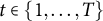
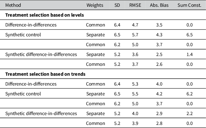
We observe this pattern in more detail when we evaluate how the RMSE develops over an increasing number of observations. The relevant aspect for the reduction in estimation error in SCMs is the number of available pre-treatment control units. Figure 2 shows that increasing the number of pre-treatment control units reduces the RMSE for all estimation approaches. It further highlights that SCMs are preferable in terms of the RMSE for both selection on trends and levels, with SDID having the best performance. When comparing common and separate weights strategies, we again observe that for SC, the common weights approach reveals some advantages, while for SDID, the two approaches have comparable RMSE values. Only in the case of treatment selection based on trends do we see slightly better rates of decreasing RMSE for common weights approaches.

Figure 2

Root-mean-squared-error (RMSE) of different estimation methods and weights. Monte Carlo simulations vary the number of pre-treatment control units (natural-log scale on the x-axis) and the treatment assignment based on levels (top row) or trends (bottom row).

Overall, the simulations confirm the central role the constant control comparison plays in ensuring the sum constraint for treatment effects on proportional outcomes. The results from the simulation study highlight that imposing separate weights across outcomes does not yield superior performance relative to the common weights estimators. This shows that enforcing the sum constraint does not come at the cost of efficiency, but ensures that the effect estimates add up.

6 Empirical applications

6.1 Climate policy and party outcomes

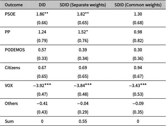
We apply our synthetic control framework to reevaluate the findings of Bolet et al. (Reference Bolet, Green and González-Eguino2024). While the original study focuses on a single party’s vote share, we analyze the full set of party vote shares as a compositional outcome. This illustrates how separate synthetic controls can generate incoherent treatment effects, and common weights resolves this problem.

Bolet et al. (Reference Bolet, Green and González-Eguino2024) study the electoral effects of a compensatory “Just Transition Agreement” in Spanish coal-mining areas using municipal election data from 2008 to 2019. Across a range of DID specifications comparing mining and non-mining municipalities in three Spanish provinces, they report a positive effect of about 1.8 percentage points on PSOE’s vote share in 2019, which they interpret as an electoral reward for the incumbent party. However, the underlying theoretical argument implies a reallocation of votes from opposition parties toward the government, raising the question of how the policy affects the full vector of vote-share proportions.

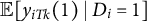
We first replicate their analysis for all major parties using a DID specification, which includes indicators for treatment status, the post-treatment period and their interaction.Footnote ¹⁴ The DID estimates in Table 2 confirm the main finding that support for the PSOE increases by around 1.86 percentage points. At the same time, we estimate a substantial decline in support for the far right VOX of roughly 3.9 percentage points. The mainstream opposition party PP also gains about 1.2 percentage points, although this effect is not statistically significant, and the remaining parties register smaller and statistically insignificant changes. As discussed above for DID, the estimated effects across all parties sum to zero, reflecting the compositional nature of vote shares.

Table 2

Estimates of the effects of the Just Transition Agreement on party vote shares (p.p.) in the 2019 Spanish elections using difference-in-differences (DID) and synthetic difference-in-differences (SDID) with separate and common weights

Note: Entries are point estimates; subrows report jackknife standard errors. * $p < 0.05$ , ** $p < 0.01$ , and *** $p < 0.001$ . N = 2,455.

We next apply SDID with separate weights. In the application, treated and control municipalities exhibit visibly non-parallel pre-treatment voting trends (see Figure 2 in Bolet et al. Reference Bolet, Green and González-Eguino2024), making SDID well suited for constructing more accurate counterfactual vote-share trajectories for each party. The SDID estimates in Table 2 are similar in magnitude to the DID results, but both PSOE and PP now exhibit statistically significant positive effects. This points to a joint mainstream gain from voter deradicalization rather than a benefit confined to the governing party. However, the estimates here no longer satisfy the compositional constraint. Summing the effects yields a net increase of $0.55$ percentage points across parties, contradicting the fact that vote shares must sum to one. This inconsistency arises because separate SDID estimates each party using outcome-specific synthetic controls, thereby comparing different counterfactuals across components of the same composition.

Finally, we apply the SDID estimator with common weights, which enforces a constant control comparison across all parties. The resulting estimates in Table 2 satisfy the sum-to-zero constraint by construction. These estimates are generally smaller than in the previous approaches, but still indicate a decline of about 3.43 percentage points for VOX. The effects on PSOE and PP remain positive, but are not statistically significant at conventional levels. This suggests that the Just Transition Agreement did not primarily benefit the governing party, but rather decreased electoral gains of the far right. This pattern is obscured when outcomes are analyzed separately, but becomes transparent once the full composition is modeled jointly with common weights.

Overall, this application demonstrates the benefits of SCMs with common weights for panel data studies with proportional outcomes. The synthetic controls with common weights maximize the fit of pre-treatment trends between control and treated units, while keeping the effects balanced with each other. Analyzing the complete set of vote shares substantively suggests that the Just Transition Agreement did not just benefit the governing party; rather, it deradicalized voters, reducing support for the far right. While our evidence complements and challenges the initial conclusions drawn by Bolet et al. (Reference Bolet, Green and González-Eguino2024), this application primarily serves to highlight how accounting for the compositional nature of vote shares allows for logically consistent and interpretable estimates across multiple proportions.

6.2 Anti-LGBTQ policies and turnout-adjusted vote shares

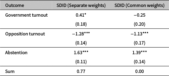
As a second application, we revisit the Polish case analyzed by Haas et al. (Reference Haas, Bogatyrev, Abou-Chadi, Klüver and Stoetzerforthcoming), who estimate the electoral effects of municipal anti-LGBTQ resolutions prior to the 2019 parliamentary elections. In their main analysis, Haas et al. (Reference Haas, Bogatyrev, Abou-Chadi, Klüver and Stoetzerforthcoming) apply SDID separately to the following voting outcomes: government turnout (votes for the ruling party divided by eligible voters), opposition turnout (votes for other parties divided by eligible voters) and overall turnout. Recasting the latter outcome as abstention, defined as the share of eligible voters who did not vote for any party, we focus on three proportions of the same whole, of the electorate. While this differs from Section 6.1, which focused on shares of valid votes, both settings are compositional.

Table 3 contrasts the original SDID with separate weights and our SDID with common weights on the full municipal panel ( $N{=}14{,}856$ ). Three differences are central. First, while the voter demobilization found by Haas et al. (Reference Haas, Bogatyrev, Abou-Chadi, Klüver and Stoetzerforthcoming) is also evident in our results, the effect becomes smaller in magnitude under common weights: $1.39$ percentage points versus $1.63$ percentage points with separate weights. Second, due to common weights, the government turnout estimate changes sign and loses its statistical significance. Third, and most consequential for interpretation, the separate-weights SDID yields effects that do not respect the composition, whereas the common-weights SDID sums to $0$ by construction. This discrepancy is large relative to the component estimates under separate weights and can distort substantive inferences across categories. In contrast, common weights deliver a coherent account of proportional outcomes: abstention increases to about the same extent as turnout for the opposition decreases, while there is little to no change on the ruling party side.

Table 3

Estimates of the effects of anti-LGBTQ resolutions on turnout-adjusted outcomes (in p.p.) in the 2019 Polish parliamentary election using synthetic difference-in-differences (SDID) with separate vs. common weights

Note: Entries are point estimates; subrows report jackknife standard errors. * $p < 0.05$ , ** $p < 0.01$ , and *** $p < 0.001$ . N = 14,856.

This second application demonstrates the practical value of using common weights to ensure coherent estimates when outcomes are proportions. It complements our first application by demonstrating the same coherence benefits in analyses where turnout is explicitly part of the outcome vector.