


1. INTRODUCTION
Taylor Glacier defies conventional definitions of a cold-based glacier by hosting a subglacial and englacial hydrologic system. Taylor Glacier (Fig. 1), in the McMurdo Dry Valleys, drains the East Antarctic ice sheet in an arid climate with mean annual air temperatures of −17.5°C and mean annual precipitation of 60 mm a−1 w.e. (Fountain and others, Reference Fountain, Lewis and Doran1999a, Reference Fountainb). The aptly named Blood Falls is an intermittent outflow of iron-rich brine that hosts an active microbial community (Mikucki and Priscu, Reference Mikucki and Priscu2007); the brine discharges at the surface on the northern side of Taylor Glacier staining the ice red and depositing a red-orange apron of frozen brine, which aggrades with each brine outflow event and partially degrades in the summer warm period. The red color results from iron oxides precipitating when the iron-bearing suboxic brine comes in contact with oxygen in the atmosphere. The brine source, inferred from thermal and flow modeling (Hubbard and others, Reference Hubbard, Lawson, Anderson, Hubbard and Blatter2004), is a putative subglacial reservoir several kilometers upstream that connects with a pervasive brine groundwater system detected from geophysical measurements (Mikucki and others, Reference Mikucki2015). Until now, a lack of evidence for active flow of englacial brine from the subglacial source to Blood Falls left this connection as speculation. Penetration and sampling of pressurized brine at Blood Falls by Kowalski and others (Reference Kowalski2016) and the MIDGE team provides direct evidence in support of our interpretations presented here. Mikucki and others (Reference Mikucki2015) show that much of the valley floor sediments are saturated with brine, leaving open the question of why subglacial brine flows supraglacially from only a single discharge point.
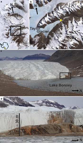
Study area. (a) Location of Taylor Glacier and Taylor Valley in the McMurdo Dry Valleys, Victoria Land, Antarctica (DigitalGlobe, 2005). (b) Location of Blood Falls (star) in Taylor Valley. (c) The central third of the Taylor Glacier terminus flows directly into Lake Bonney. Blood Falls is located in the northern third of the terminus. Supraglacial valleys incised by summer melt are present on the glacier surface. (d) The ice cliff and terminal moraine covered by a frozen apron of Blood Falls outflow deposits. Smaller crevasse-like structures of frozen brine outcrop on the surrounding cliff faces.

The existence of an active hydrologic system in Taylor Glacier has broad implications for cold-based glacial systems and local influences on the McMurdo Dry Valleys (Carr and others, in prep). Glacial hydrologic systems can be responsible for basal sliding, melt, and softer ice more susceptible to deformation (Benn and Evans, Reference Benn and Evans2010). Evidence for water in cold-based glaciers may require changes to glacier dynamics models especially in the polar regions. The Blood Falls hydrologic system has local influences on microbial activity, geochemical reactions, and the transport of potential nutrients within Taylor Valley (Mikucki and others, Reference Mikucki, Foreman, Sattler, Lyons and Priscu2004, Reference Mikucki2009). Beneath a glacier, subglacial water increases basal erosion rates (Benn and Evans, Reference Benn and Evans2010) and Taylor Glacier's subglacial brine, in particular, increases nutrient transport into Lake Bonney, thereby affecting microbial nutrient access (Mikucki and others, Reference Mikucki, Foreman, Sattler, Lyons and Priscu2004; Lyons and others, Reference Lyons2005). The mechanisms by which the brine exits the subglacial environment control the nutrients available for microbial activity because the brine undergoes geochemical reactions with the bedrock, sediment, ice, and water (Mikucki and others, Reference Mikucki, Foreman, Sattler, Lyons and Priscu2004, Reference Mikucki2009). With better knowledge of pathways and residency times as brine flows through the subglacial and englacial environments, this study can bring us closer to understanding the coupled geochemical evolution of and microbial environment hosted by the brine.
In this study, we use radio echo sounding (RES) and hydraulic-potential modeling to map the englacial and subglacial pathways, respectively, which bring brine to the surface. While artesian water discharges are rare in cold glaciers, Blood Falls lies along a spectrum of possible hydrologic systems that can help us understand the evolution and persistence of liquid water pathways in cold glacial ice. Studies of hydrologic systems in the Arctic have found that summertime supraglacial meltwater can reach the bed of cold-based, polythermal glaciers and develop subglacial drainage systems (Boon and Sharp, Reference Boon and Sharp2003; Bingham and others, Reference Bingham, Nienow, Sharp and Boon2005). Boon and Sharp (Reference Boon and Sharp2003) show this occurs when freezing of meltwater in initial crevasses warms the surrounding ice and increases the probability that subsequent crevassing will penetrate to the bed. Other studies in Antarctica show potential for hydrologic connections between known subglacial lakes beneath the East Antarctic ice sheet (Wright and others, Reference Wright2012; Wolovick and others, Reference Wolovick, Bell, Creyts and Frearson2013). They attribute the presence of subglacial water in this cold region to warmer basal conditions beneath thick ice from trapping of geothermal and frictional heat. Taylor Glacier differs from the polythermal Arctic glaciers by a lack of persistent temperate ice and differs from the Antarctic ice sheets by its relative thinness.
2. BACKGROUND
2.1. Study area
As an outlet glacier of Taylor Dome on the East Antarctic ice sheet, Taylor Glacier flows over 100 km through the Trans-Antarctic Mountains eastward through Taylor Valley (Robinson, Reference Robinson1984; Higgins and others, Reference Higgins, Hendy and Denton2000b). The central portion of the glacier enters directly into the west lobe of Lake Bonney, a saline lake with a perennial ice cover (Fig. 1c). Ice-cored lateral and terminal moraines wrap around the terminus from the north-facing ice cliffs to where the ice flows eastward into the lake. To a lesser extent, shorter ice-cored moraines also wrap around the south-facing ice cliffs. A thick layer of debris-laden basal ice is conspicuous in the south-facing ice cliffs, but less obvious on the north side due to a large apron of calved ice blocks at the ice cliff base.
Although most of Taylor Glacier's ablation occurs through calving and sublimation (Hoffman and others, Reference Hoffman, Fountain and Liston2008; Pettit, in prep), summer melt does occur on the lower portion of the glacier. Three large surface valleys (up to 30 m deep and >100 m wide ridge-to-ridge at the surface) with ephemeral summertime streams dominate the surface relief in the lower terminus region (Robinson, Reference Robinson1984; Pettit and others, Reference Pettit, Whorton, Waddington and Sletten2014; Fig. 1c). These valleys begin as shallow, narrow surface depressions 1100 m upglacier from the terminus where summer melt becomes a non-negligible component of surface ablation (Johnston and others, Reference Johnston, Fountain and Nylen2005).
As a glacial feature within ice flowing at 3 m a−1, the appearance of Blood Falls changes annually (Black and others, Reference Black, Jackson and Berg1965; Black and Bowser, Reference Black and Bowser1968; Mikucki and others, Reference Mikucki, Foreman, Sattler, Lyons and Priscu2004; Carmichael and others, Reference Carmichael, Pettit, Hoffman, Fountain and Hallet2012). Brine outflow events add layers of frozen deposits to the brine apron, often expanding the visible extent of the apron. Ablation of the apron concentrates oxidized iron, while meltwater transports iron deposits into Lake Bonney. Cracks in and upstream from Blood Falls open as the glacier flows; some act as an outflow point for brine. Streaks of red-orange frozen brine outcrop on the ice cliffs next to Blood Falls and occasionally are found elsewhere (Keys, Reference Keys1979). Despite this variability in appearance, the location of Blood Falls as the primary discharge site at the north end of Taylor Glacier's terminus has remained unchanged since early observations (Black and others, Reference Black, Jackson and Berg1965).
2.2. Basal conditions of Taylor Glacier
Subsurface geology of Taylor Valley is mostly constrained by several boreholes drilled in the 1970s in the eastern part of the valley as part of the Dry Valley Drilling Project (DVDP). Unfortunately, the borehole closest to the terminus of Taylor Glacier was drilled ~20 km away, near Lake Hoare. Marine deposits, ranging in age from approximately 7–4.6 million years BP, show that at least the eastern part of Taylor Valley was a deep-water fjord reaching 600–900 m depth before it was filled in by sediments (Elston and Bressler, Reference Elston and Bressler1981). Coarse, water-lain glacial deposits on the valley floor show evidence of subaerial erosion indicating a shallowing and emergence of the fjord (2.4–1.8 million years BP) possibly due to valley floor uplift or recession of the Ross Sea Embayment (Elston and Bressler, Reference Elston and Bressler1981). Lyons and others (Reference Lyons2005) hypothesize that overdeepened areas along the valley floor from earlier glaciations trapped Miocene-age seawater, leading to the formation of a large saline lake. They further hypothesize that Taylor Glacier advanced over this inferred lake in the early Quaternary. The Blood Falls source brine, along with some salts in Lake Bonney, may be vestiges of this ancient lake (Black and others, Reference Black, Jackson and Berg1965; Higgins and others, Reference Higgins, Denton and Hendy2000a; Lyons and others, Reference Lyons2005).
Hubbard and others (Reference Hubbard, Lawson, Anderson, Hubbard and Blatter2004) used RES-derived bed topography and bed reflection power, thermal and flow modeling of the glacier, and hydraulic-potential models of the bed to suggest subglacial ponding of brine several kilometers upstream from Taylor Glacier's terminus. High bed-reflective-power is typically used as a signature of subglacial water because water has a high relative permittivity compared with ice. Thermal and flow modeling predict basal ice temperatures underneath the glacier (−7.8°C in the overdeepening and −18°C at the northernmost margins of their study area). They used the overlapping locations of high bed-reflective-power and −7.8°C bed temperatures as an indicator of ponding subglacial, saline water. With additional hydraulic-potential calculations they located the putative subglacial brine under 400–500 m of Taylor Glacier ice in an overdeepened part of the bed estimated to be a 75 m deep depression more than 1 km wide. This bed depression is located 3–6 km upglacier of the terminus based on their RES-derived bed topography. Their analysis, however, cannot distinguish if the brine exists as ponds, saturated sediment, or a thin film along the bed. For the chemical constituents of seawater, a salinity of ~125‰ is required to depress the freezing point of brine to −7.8°C at pressures of 30–300 m of ice (Doherty and Kester, Reference Doherty and Kester1974).
Mikucki and others (Reference Mikucki2015) used an airborne transient electromagnetic sensor to infer that a body of brine-saturated sediments extends from at least 6 km upstream of Taylor Glacier's terminus into Lake Bonney. They further concluded that Blood Falls outflow requires this upstream brine supply to exist. The absence of brine outflow emerging from other glaciers in Taylor Valley (mountain glaciers draining the Asgard Range and Kukri Hills) supports the model that Blood Falls brine is sourced from the valley floor subglacial sediments.
At the base of Taylor Glacier, a significant debris-rich basal-ice layer acts as a transition to the underlying substrate. Pettit and others (Reference Pettit, Whorton, Waddington and Sletten2014) estimate this extensive layer of basal ice to be 10–15 m thick and 20–40 times softer than clean, cold, meteoric glacier ice. They propose the deformation of this layer as a mechanism to explain Taylor Glacier's surface speeds that are 20 times greater than what Glen's flow law (Glen, Reference Glen1958) predicts for cold, thin ice. This basal-ice layer varies spatially in thickness and effective viscosity, as inferred from ice thickness and surface speeds (Pettit and others, Reference Pettit, Whorton, Waddington and Sletten2014). Its low effective viscosity may be due to the presence of salts in the basal-ice and underlying sediments; we expect, therefore, faster ice flow above areas of subglacial brine-saturated sediments.
2.3. Using RES to image water within glaciers
RES data can be used to find changes in the properties of ice, such as average electromagnetic wave speed along the signal path and material permittivity. Permittivity values of a material such as ice or water are highly dependent on temperature, salinity, and, especially for saline solutions, the frequency of the emitted electromagnetic wave. Permittivity values are found experimentally and thus, in this study, we use relative permittivity values for freshwater, seawater, and meteoric ice from previous studies (86 for freshwater, Davis and Annan, Reference Davis and Annan1989; 80 for seawater and 3.2 for −40°C ice, Smith and Evans, Reference Smith and Evans1972) that are close to but may not be the actual permittivity values for the specific combinations of temperature and salinity for Blood Falls brine and ice at all stages through the hydrologic system.
Brine, like water, has a high permittivity value that causes it to reflect electromagnetic wave energy. Pockets of brine or water that are similar size to the wavelength will scatter the energy and obscure the reflections below. Previous studies have inferred brine or water as both layers and pockets within ice (Smith and Evans, Reference Smith and Evans1972; Murray and others, Reference Murray2000; Barrett and others, Reference Barrett, Murray, Clark and Matsuoka2008). Smith and Evans (Reference Smith and Evans1972) found that internal layers of brine-infused ice in ice shelves cause a horizontal zone of scattered reflections that mask the high-amplitude reflection off the ice shelf bottom. Murray and others (Reference Murray2000) collected RES transects on Bakaninbreen Glacier, Svalbard and found a horizontal scattering zone below which the bed reflector was either obscured or downwarped. They ascribe this obscuring and downwarping of the bed reflector respectively to the scattering effect of water-saturated ice and a decrease in wave propagation velocity through the scattering layer. These properties of brine-related scattering allow us to calculate wave speed and material permittivity from increased travel time to a high-amplitude, downwarped, horizontal reflector.
3. METHODS
3.1. RES field methods and data processing
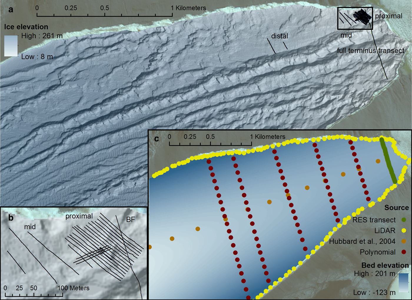
We collected three groups of RES transects, a group ‘proximal’ to Blood Falls (within 80 m), a ‘mid’ group farther up-glacier (100–160 m), and a ‘distal’ group 800–1000 m up-glacier from Blood Falls, in order to constrain the full extent and geometry of the bed and any englacial brine (Figs 2a, b). We also collected an additional 600 m transect across the full width of the terminus to resolve any larger-scale englacial and subglacial features (Fig. 2a). The proximal group consisted of 16 transects perpendicular to the ice flow direction (hereafter, ‘cross-flow transects’) and three transects parallel to the ice flow (‘along-flow transects’). The cross-flow transects were spaced 5 m apart and ranged from 85 to 125 m long. The mid group contained three cross-flow transects and the distal group contained two cross-flow transects.
Surface and bed topography of Taylor Glacier. (a) 2 m LiDAR digital elevation map from NASA/USGS (Schenk and others, Reference Schenk2004) with black lines showing RES transects. (b) Inset is an enlargement of the RES transect locations. BF marks the location of Blood Falls. (c) Calculated bed topography based on measurements (green circles are RES derived, yellow circles are LiDAR derived), approximations (orange circles are from analysis by Hubbard and others, Reference Hubbard, Lawson, Anderson, Hubbard and Blatter2004), and calculations (red circles are calculated hyperbolas derived from the LiDAR and Hubbard and others, Reference Hubbard, Lawson, Anderson, Hubbard and Blatter2004). Base map imagery from DigitalGlobe (2005).
To collect the RES data, we used a 100 MHz pulseEKKO PRO ground-penetrating radar with a 1 m wavelength and stacked 64 monopulses recorded at 0.1 ns intervals. We collected every transect using a common-offset mode. Along each transect, traces were collected every 0.25 m in order to make the horizontal resolution approximately equal to the vertical resolution (one quarter wavelength), however, the full-terminus transect had a trace spacing of 0.5 m.
To process the RES data, we use MATGPR_R3 (Tzanis, Reference Tzanis2010), a script run within MATLAB (Mathworks, Inc.). We applied an FK migration using a uniform 0.167 m ns−1 for the wave propagation velocity through cold ice. We topographically corrected each transect using a precision differential GPS in the WGS 1984 geographic coordinate system with an ITRF ellipsoid vertical datum. Horizontal errors are typically ± 0.02 m, but never exceed ± 0.04 m and vertical errors are typically ± 0.04 m, but never exceed ± 0.08 m. A local GPS base station on the northern shore of the west lobe of Lake Bonney provides differential GPS correction (benchmark TP02, latitude: −77.72°, longitude: 162.27°, elevation: 18.4 m).
To define the location of the englacial brine (manifested as a scattering zone in the RES data), we examine each migrated transect, outline the main cluster of the scattering zone points, and pick the visual center of the zone. We also pick the basal reflection from each migrated transect. Using the GPS data and a calculation of depth, by assuming wave velocity of 0.167 m ns−1, we obtain the 3-D location of the scattering zone and basal reflection. Though RES records reflections from off-nadir features, many of these off-nadir returns are interpretable as such, including returns from nearby cliffs and survey stakes. We present the scattering zone and basal reflection assuming they arise from the nadir direction.
3.2. Water content calculations
A zone of ice that has anomalous electrical properties compared with the surrounding ‘normal’ glacier ice will alter the velocity of electromagnetic waves. Where the zone overlies a distinctive reflector, we can infer the difference in ice properties from relative downwarping of the reflector due to contrasting electromagnetic wave speeds (Murray and others, Reference Murray2000). Downwarping features only appear in our RES data directly below scattering zones, which we interpret as zones of anomalous electrical properties. For this study, we assume the downwarping is not a physical aspect of the basal-ice geometry and is instead caused entirely by the spatial variations in ice properties because elsewhere the basal-ice/clean-ice interface is smooth and relatively flat on comparable length-scales.
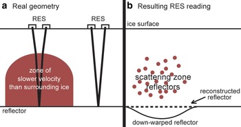
A decrease in wave speed through water-saturated, brine-saturated, or temperate ice can cause an apparent downwarping of a basal reflector (Murray and others, Reference Murray2000). We use the amount of apparent downwarping in the basal reflector of our unmigrated, topographically corrected RES profiles to calculate the concentration of water within the scattering zone using relative permittivity values for both freshwater and seawater. Figure 3 shows a cartoon diagram of ray paths for the signal going through cold, dry meteoric ice versus through warm, wet, or salty ice relative to the downwarped reflector. In this analysis, we assume that the cold, dry meteoric ice transmits electromagnetic waves with velocities of 0.167 m ns−1. The 1 m offset between the transmitter and receiver contributes a subcentimeter error in derived depths for englacial and subglacial features when using one-way travel times rather than the true vertical travel times. We do not explicitly correct for this error. Additionally, we assume that the scattering zone extends vertically down to the reconstructed downwarped reflector. If the scattering zone is more limited in its vertical extent, then the estimates of velocity will be lower to achieve the same travel time. This assumption is critical to our results and is discussed in Section 4.2.
Cartoon diagram of apparent reflector geometry as a function of differing ice properties. This illustrates a cause of the downwarping seen in Fig. 4a. (a) A geometrically horizontal reflector crosses under an englacial zone of water-rich ice. RES pathways pass through both the water-rich zone and the clean, meteoric surrounding ice. (b) The apparent geometry of the horizontal reflector, as imaged by RES, is affected by the slower velocity of electromagnetic waves through brine- or water-rich ice.

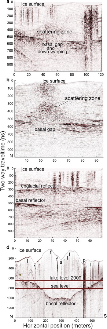
Examples of topographically-corrected RES transects. (a) Unmigrated cross-flow transect from the proximal group showing the basal reflector, downwarping, and gap in the basal reflector and the scattering zone. (b) Cropped and migrated display of data in (a). (c) Unmigrated, along-flow transect from the proximal group showing the basal reflector as well as the englacial horizontal reflector referred to in the text. (d) Full-terminus transect showing the scattering zone (star) at the northern edge of the terminus. The basal reflector dips below the 2009 Lake Bonney water level and modern sea level (marked by red lines). The vertical reflections are marked by letters denoting the cause for the reflection: ‘p’ for meltwater pond, ‘s’ for surface meltwater, ‘f’ for data file transition, ‘l’ for topographic low that collects meltwater.

The wave propagation velocity in the scattering zone is calculated by:
 $$v_{\rm z} \; = \; \displaystyle{{(t_{\rm z} v_{\rm i} )} \over {(t_{\rm z} + t_{\rm d} )}},$$
where v z is the velocity of electromagnetic waves through the scattering zone; v i is the velocity of electromagnetic waves through the cold, dry glacier ice; t z is the approximated one-way travel time from the top of the scattering zone through cold, dry glacier ice to the reconstructed downwarped reflector; and t d is the approximated one-way travel time between the reconstructed downwarped reflector and the imaged downwarped reflector. The numerator of Equation (1) defines the real vertical thickness of the scattering zone in meters and the denominator is the total travel time from the top of the scattering zone to the downwarping seen in the profile. We apply Equation (1) to several locations of downwarping along 15 proximal transects. To reconstruct the downwarped reflector, we use points along the unwarped reflector to extrapolate the missing section of unwarped bed using a third-order polynomial curve.
We estimate percent water content by volume (W) using this equation:
 $$W = 300\displaystyle{{(c/v_{\rm z} )^2 - \varepsilon _{\rm d}} \over {\varepsilon _{\rm w}}}, $$
which applies to dispersed water (freshwater or seawater) within ice (Macheret and others, Reference Macheret, Moskalevsky and Vasilenko1993). In this equation, c is the speed of light in a vacuum, v z is as derived in Equation (1), ε d is the relative permittivity of cold dry ice (~3.2), and ε w is the relative permittivity of freshwater or seawater (~86 for fresh meltwater and ~80 for seawater; Smith and Evans, Reference Smith and Evans1972; Davis and Annan, Reference Davis and Annan1989). These values of relative permittivity for freshwater and seawater are best estimates based on previous research; we have not measured permittivity on either the ice or the brine specifically for this study and thus we can only estimate the englacial brine content. We calculate freshwater and saltwater volumes as minimum brine content and compare the values to provide an estimate of how calculated water content varies with salinity.
While picking the downwarped reflector position to use in Equations (1) and (2), we also pick the approximate horizontal center of the scattering zone to calculate the distance to each picked downwarped location. The center of the scattering zone is not easily defined and this introduces some error into the distance calculation. We assume that the processes generating the scattering zone and downwarping act primarily perpendicular to the central axis of the scattering zone; therefore, we measure all distances from the center of the scattering zone to the downwarped locations along the same transect. If a downwarped location is affected by processes operating obliquely to the transect line, then positive or negative error may be introduced into our calculation of the brine content.
3.3. Hydraulic-potential and pathways modeling
We apply Shreve's (Reference Shreve1972) equation for subglacial hydraulic potential to the terminus region of Taylor Glacier to show how subglacial brine may travel from the subglacial source towards Blood Falls:
 $$\varphi \; = \; \rho _i g\; \Big(\,fS + \Big(\displaystyle{{\rho _b} \over {\rho _i}} - f\Big)B\Big)\comma$$
where φ is the hydraulic potential (Pa); ρ b and ρ i are the density of surface brine (1100 kg m−3; Mikucki and others, Reference Mikucki, Foreman, Sattler, Lyons and Priscu2004) and glacier ice (917 kg m−3), respectively, such that the ratio ρ b/ρ i = 1.2; B is the bed elevation (m); S is the ice surface elevation (m); g is the acceleration due to gravity (9.8 m s−2); and f is a factor between 0 and 1 indicating the extent to which water follows bed topography or is pressurized by overburden due to overlying ice (f = 0 indicates no overburden effect, while f = 1 indicates full overburden). We assume a value of f = 1, and thus an average effective pressure of zero. This average value allows for local fluctuations of over- or under-pressurized brine and does not necessarily imply a floating lower terminus region. Other processes, such as active brine-saturated sediment compaction, could arguably decrease the overburden effect; however, we find f = 1 to be a reasonable assumption. Similar patterns persist throughout a range of f values from 0.5 to 1.0, which shows the robustness of our analysis.
To apply Equation (3) to Taylor Glacier's terminus region, we use ice surface elevations from NASA/US Geological Survey's (USGS) LiDAR 2 m DEM ( Schenk and others, Reference Schenk2004). With limited indications of bed elevation, we assume a parabolic bed shape (Fig. 2c) based on our data and bed topography reported by Hubbard and others (Reference Hubbard, Lawson, Anderson, Hubbard and Blatter2004) that demonstrate a relatively smooth and nearly U-shaped bed in the lower 3 km of the glacier terminus. To recreate this parabolic bed surface for Taylor Glacier, we apply a second-degree polynomial-trend interpolation in ESRI ArcGIS that is tied to approximate bed elevations. These approximate bed elevations include locations within 2 m of the glacier edge from the surface DEM (DEM vertical error is 0.3 m; ice cliffs, debris aprons, and moraines cause additional vertical error in these points at some locations); our RES full-terminus transect basal-ice reflector (0.25 m error); and approximated elevations from Hubbard and others (Reference Hubbard, Lawson, Anderson, Hubbard and Blatter2004) (75 m error as stated by the authors). Bed-elevation error changes spatially; the most precise elevations are located near our RES full-terminus transect and errors increase up-glacier. The thickness of the underlying debris-laden basal-ice layer described by Pettit and others (Reference Pettit, Whorton, Waddington and Sletten2014) is not constrained by RES data and further complicates error estimation. We assume this basal ice is impermeable and has a relatively uniform thickness throughout the modeled area; therefore, it has a negligible effect on the hydraulic-potential gradient.
We interpolate bed topography to 30, 60, 90, and 120 m grid cells, downsample the surface DEM, and create new surface and bed DEMs that vary in resolution depending on local ice thickness. This ensures that our hydraulic-potential model remains within the bounds of Shreve's (Reference Shreve1972) assumption that subglacial hydraulic potential is not affected by ice surface features smaller than the thickness of the glacier.
To calculate subglacial hydraulic potential we use algorithms in ESRI ArcMap to calculate hydraulic gradient and gradient direction from the ‘filled’ and averaged hydraulic potential (see next paragraph for a description of sink filling). The hydraulic gradient is a slope calculation that assesses the overall slope for a cell using all eight surrounding cells (Burrough and McDonell, Reference Burrough and McDonell1998). The gradient direction is an aspect calculation that finds the down-dip direction of the slope (Burrough and McDonell, Reference Burrough and McDonell1998).
Using ESRI ArcMap's embedded gradient-descent algorithm (or steepest descent; Jenson and Domingue, Reference Jenson and Domingue1988), we evaluate the flow directions for subglacial brine. Because of the uncertainty in our bed DEM, our hydraulic-potential map contains local minima that are unlikely to be real. For this calculation, therefore, we assume that all brine eventually flows out from the glacier and we force the flow directions to bypass local minima (sinks) in hydraulic potential by increasing the values within the local minima (filling the sinks; Tarboton and others, Reference Tarboton, Bras and Rodriguez–Iturbe1991) until a defined flow direction is determined. Flow at the glacier edge is allowed to exit the glacier only if no favorable hydraulic-potential pathway exists under the glacier. Once flow directions are defined, we estimate the contributory subglacial drainage patterns and relative discharge in ArcMap. The algorithm assumes that each grid cell contributes an equal volume of brine and each cell receives the integrated volume fed to it from upstream pathways. Because this assumption does not allow for areas of subglacial freeze-on and melting, we focus our discussion on the predicted hydraulic pathways rather than the predicted relative discharge fluxes.
Uncertainty in bed topography causes errors in our hydraulic potential and hydraulic-pathways; however, ice-thickness-scale topographic features are required to significantly alter hydraulic pathway locations. Based on the smoothness of basal reflectors (data from this study; Hubbard and others, Reference Hubbard, Lawson, Anderson, Hubbard and Blatter2004; Pettit and others, Reference Pettit, Whorton, Waddington and Sletten2014), as well as reports of unlithified subglacial sediments (Higgins and others, Reference Higgins, Hendy and Denton2000b), we have no reason to suspect that the actual bed has ice-thickness-scale topographic features affecting the hydraulic pathways. For hydraulic-potential calculations using f = 1, the bed elevations have about five times less impact than the surface elevations given the density difference between brine and glacier ice. Thus, we expect that errors in bed topography minimally affect the location of the hydraulic pathways. In some places, particularly upstream and on the south side of the glacier, the hydraulic potential calculated near ice cliffs may cause local redirection of flow pathways due to ice thickness that is of the same order as error in the bed topography. These local redirections, however, do not affect the larger pattern of flow.
To test the sensitivity of the pathways to uncertainty in the bed topography, we apply noise to our bed DEM by adding a randomly generated percentage of the estimated glacier thickness to the bed elevation at each point. The randomly generated percentage error induced by this noise has a normal distribution with a standard deviation of 5%, resulting in a range between −20% and +20%. We performed the calculations for hydraulic potential and hydraulic pathways described above with five trials of added artificial noise.
4. RESULTS
4.1. Mapping the scattering zone
Our RES transect data (Fig. 4 shows a representative subset) generally show a surface reflector, a basal reflector, and different mid-depth reflectors depending on the transect orientation and length. A high-amplitude, subhorizontal reflector appears 285–585 ns after the airwave arrival in the cross-flow RES transects of the proximal, mid, and distal groups (Fig. 4a is an example). We interpret this reflector as the transition between debris-free meteoric ice and the softer, debris-rich basal-ice layer described by Pettit and others (Reference Pettit, Whorton, Waddington and Sletten2014). Although we term this as the ‘basal reflector,’ it masks a lower transition to ice-rich sediments or bedrock below. Two dipping reflectors on the left side of Fig. 4a may be multiples or be caused by nearby ice cliffs. A break in the basal reflector occurs in most transects directly below a localized englacial scattering zone (Fig. 4a). Beginning up-glacier, the distal transects show a continuous basal reflector and no detectible englacial scattering. In the mid transects, as many as two weak scattering zones appear. Closer to Blood Falls, each of the sixteen cross-flow transects of the proximal group have a single scattering zone appearing near the center of the transect (Fig. 4a).
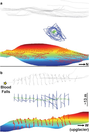
By picking the outline and center of the scattering zone for 15 of the proximal transects (from migrated transects, e.g. Fig. 4b), we define the scattering zone as a subhorizontal zone elongated in the direction of ice flow (Fig. 5). In Fig. 5, the scattering zone is defined within the context of glacier surface topography (from GPS) and bed topography (interpolated from the picked basal reflectors).
Outline of scattering zone. The small black points identify GPS points used to define the glacier surface. Red points identify RES-picked points used to define the basal topography. Shading shows interpolated basal topography, with color denoting interpolated elevations (red is high and blue is low). Blue lines outline the scattering zone in each migrated RES transect. The green line connects the approximate centers of the migrated scattering zones on each transect defining the central axis of the scattering zone. (a) Subparallel to ice flow, this view of the scattering zone from Blood Falls looks up-glacier into the ice. (b) This cross-flow view of the scattering zone has Blood Falls to the left and looks across the glacier from north to south. Note that although these figures suggest a cylindrical conduit shape, this is solely a product of how we chose to define the edges of the scattering zone.

The along-flow transects were collected near where we observe the trending scattering zones in the proximal cross-flow transects. All three along-flow transects lack detectable scattering zones; show a piecewise basal reflector; and prominently display a high-amplitude, piece-wise, horizontal, linear, englacial reflector (Fig. 4c). These three observations suggest that the scattering zones have along-flow continuity: the englacial horizontal reflector in the along-flow transects may correspond to the top of the scattering zone where the permittivity contrast between wet, warm and/or salty ice and meteoric ice is highest. Some subhorizontal reflections may also arise from short, 2–3 m-high ice cliffs 20–40 m away.
The full-terminus transect (Fig. 4d) shows a relatively smooth, U-shaped basal reflector, a break in the basal reflector near Blood Falls and several locations of strong vertical ringing. A ghost of the surface reflector appears near the basal reflector and is an artifact.
The vertical ringing seen in Figs 4a, c-d results from meltwater ponds, or other surface melt or meltwater collection areas, or metal survey stakes that mark file transitions. The broad vertical ringing (labeled ‘p’ in Fig. 4d), is at the bottom of the southernmost supraglacial valley and results from a large, ice-covered meltwater pond crossed by the transect. Other vertical reflections result from metal stakes at data file transitions (‘f’), known surface melt locations (‘s’), or topographic lows (‘l’) that are likely to collect meltwater during the austral summer when we acquired the data. We interpret these meltwater features as seasonal surface features that refreeze or ablate each winter, due to their localized effect on the radar. The surface ablation rate in this region averages 0.5 m a−1 (Pettit and others, Reference Pettit, Whorton, Waddington and Sletten2014) and, thus, shallow surface ponding and related latent-heat effects are unlikely to affect ice at depth.
4.2. Spatial pattern of brine content
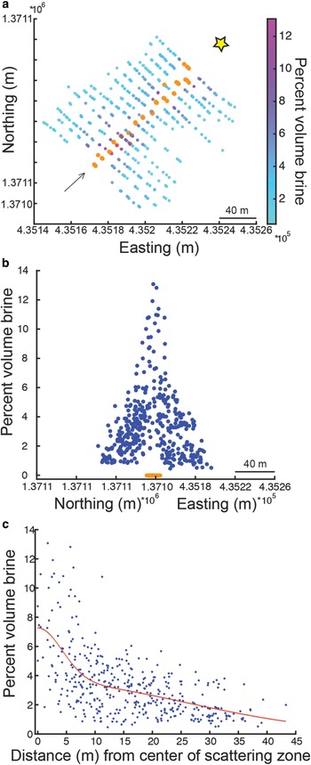
Analysis of brine content derived from RES scattering and basal-reflector downwarping (Fig. 6) shows percent volume of brine at increasing horizontal distance from the center of the scattering zone outlined in Fig. 5. Figure 6a shows the brine content in map view; dots represent basal reflection locations that we used to calculate brine content, with brine content represented by the light blue (low brine content) to dark purple (high brine content) scale. The orange points in Figs 6a, b represent the three picks of the center of the scattering zone for each transect; there is no calculated brine content for these center points due to the disappearance of the basal reflector under the center of the scattering zone. Figure 6b shows brine content as a function of horizontal distance; the figure is oriented along the arrow in Fig. 6a, the central axis trend, showing that brine content increases towards the center of the scattering zone. Figure 6c shows the brine content in each transect relative to the distance from the respective transect center point (orange dots in Fig. 6a). This adjusts for the slight variations of each transect center to the mean central axis of the scattering zone. We fit a two-term Gaussian model to this scatter plot to capture the transition between two different zones apparent in these data.
Spatial variation of percent volume of brine using seawater as a proxy. (a) Map view showing brine content from low (light blue) to high (dark purple) in relation to the centers of the scattering zone for each transect (orange points). The star shows approximate location of the top of Blood Falls. The arrow gives reference for the orientation of part (b) along the central axis. (b) Along-arrow view from part (a) shows brine content on the vertical axis and the map plane on the horizontal axes. Orange points are the centers of the scattering zone for each transect. (c) Brine content as a function of distance from the center of the scattering zone (orange points) in each transect (note this distance reference is different than in (b)). The red line shows the two-part Gaussian model.

The two-term Gaussian fit suggests two simultaneously acting processes – one broadly acting process generates the points far from the center and fits best to a Gaussian with a standard deviation of 18 m and another narrowly acting process near the central axis of the scattering zone with a standard deviation of 3.0 m (Fig. 6c). The transition in dominance of the two Gaussian terms occurs 7.3 m from the central axis of the zone. The far Gaussian process has a brine content of 2.8% at one standard deviation, while the near Gaussian term has a brine content of 6.4% at one standard deviation. Within 2 m of the central axis our measurements reach a peak of 13%, however, the scattering completely obscures the basal reflection in many places, making brine content impossible to measure. While we fit brine content measurements near the central axis with a Gaussian, the process may, in fact, be exponentially approaching 100%, as evidenced by the sampling of liquid brine in one location (Kowalski and others, Reference Kowalski2016).
These brine content estimates assume the salinity of seawater. There is a direct relationship between the water content estimation and the salinity; therefore, higher salinity brine would result in higher brine-content values than we present here.
The spatial scatter in the brine content (standard deviation of 1.7 from the two-term Gaussian model) results from both methodological factors and real variability. Human bias in picking the downwarped and non-downwarped basal reflector is a minimal source of error since three trials produced mean velocities by transect within 0.005–0.01 m ns−1. The real width of the scattering zone and the local brine content within the scattering zone naturally varies spatially. This natural variability indicates that the process responsible for englacial brine emplacement is stochastic and generates statistical variability in the brine content.
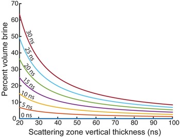
In some transects, increased attenuation and wave scattering due to thicker ice or a more pronounced scattering zone mask more of the downwarped basal reflector and eliminate our ability to estimate brine content near the central axis of the scattering zone. For those transects where the downwarping basal reflector is completely masked due to wave scattering, we infer that the brine content is significantly higher. We also note that our brine-content estimates are minimum magnitudes because (a) our calculations use the salinity of seawater, but we estimate the brine to be ~3.5 times more saline than seawater and (b) our assumption that the scattering zone extends to the bed may be incorrect. By modifying the assumed geometry (shown in Fig. 3) to allow measurable thickness of fresh meteoric ice underneath the scattering zone, we calculate as much as 60% brine content along the central axis (Fig. 7). By any method, thinning the scattering zone in vertical extent has a significant effect on the brine-content estimate (Fig. 7). For an extreme downwarping of 30 ns, for example, thinning the effective scattering-zone thickness from 80 to 40 ns more than doubles the brine content responsible for the downwarping. This effect is shown for a range of downwarping by varying possible one-way travel times between 0 and 30 ns in steps of 5 ns (Fig. 7). The typical assumed scattering zone one-way travel time is 50–100 ns.
The effect of scattering zone vertical thickness on the estimated brine content. Each line shows this effect for a different amount of downwarping in the underlying basal reflector (measured in one-way travel time).

4.3. Hydraulic-potential and brine-pathway models
Subglacial hydraulic-potential modeling allows us to estimate brine routing as it flows from high to low potential along the steepest gradient (Fig. 8). Figure 8 shows hydraulic potential averaged over five trials with artificial noise added to the bed topography and it displays an overall trend of brine flow down-glacier towards the terminus. Deviations from this trend reflect the greater influence of surface topography over bed topography in routing brine along pathways. Each of the five trials with artificially added noise individually show similar trends as the average of the trials shown in Fig. 8. The gradient and gradient direction are derived from the averaged hydraulic potential. The trends also persist at f = 0.75 and f = 0.5, which have greater influence from the bed and show increasing routing of brine from the sides of the glacier towards the center. The trends breakdown at f = 0.25 when the bed has over three times more influence than the surface topography.
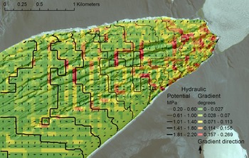
Subglacial hydraulic-potential gradient model. This is an average of five trials in which each trial has artificial noise added to the bed topography (one standard deviation is 5%). The model varies resolution with estimated ice thickness. The hydraulic-potential gradient is calculated by the change in potential (MPa) over distance and is shown as high gradient (red) to low gradient (green). The arrows are a 90 m average gradient direction of the surrounding cells. The contours show hydraulic potential (MPa) from low (thin contours) to high (thick contours) potential. Base map imagery from DigitalGlobe (2005).

In the brine-pathways model, our assumption of contributory flow precludes finding distributary braided channels, as suggested by Catania and Paola (Reference Catania and Paola2001). Despite this limitation, our results show possible active hydraulic pathways that direct subglacial brine along the northern half of the glacier towards Blood Falls. This trend is consistent across most of the five trials with added artificial noise and is definitively apparent when all five are averaged (Fig. 9). To compare the modeled brine pathways with possible discharge locations, we mapped these pathways along with the spatial extent of the ice-cored moraines (light brown in Fig. 9), the location of past known Blood Falls discharge activity (GPS coordinates provided by personal communication T. Nylen), and the lateral extent of the scattering zone.
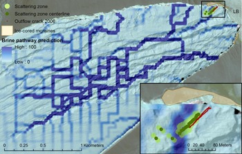
Subglacial hydraulic-pathways predicted from hydraulic-potential calculation (Fig. 8). Darker blue indicates greater likelihood for brine flow channelization. The terminal ice-cored moraines (light brown), lateral extent (light green) and central axis (dark green) of the scattering zone, and 2006 brine outflow crack (red, personal communication T. Nylen) are shown and magnified in the inset. DigitalGlobe (2005) imagery shows the location of Lake Bonney (LB).

5. DISCUSSION
5.1. Englacial pathway brings brine to Blood Falls
Our RES data suggest that concentrated, englacial liquid near Blood Falls causes a significant change in the dielectric properties of the ice and is scattering the electromagnetic wave energy. We conclude that this englacial liquid is brine because (a) Kowalski and others (Reference Kowalski2016) penetrated brine close to the scattering zone, (b) iron-rich brine emerges locally from the surface during Blood Falls release events (Carr and others, in prep; Mikucki and others, Reference Mikucki2009), and (c) Mikucki and others (Reference Mikucki2015) infer an extensive reservoir of brine beneath Taylor Glacier based on conductivity measurements. The englacial brine zone we imaged by RES is interpreted as the previously unknown link between the putative subglacial reservoir of brine and its intermittent supraglacial outflow, Blood Falls.
The 3-D boundary of the scattering zone we outline in Fig. 5 shows one primary subhorizontal volume of englacial brine elongated in the direction of ice flow with its central axis extending upstream from the Blood Falls brine apron. Our mid-RES transects additionally suggest probable confluence of tributary pathways of the englacial brine.
Despite this evidence for an extensive englacial brine network, the brine does not travel far englacially before freezing because it is not initially in thermal equilibration with the glacier ice as shown by the 10°C temperature difference between brine (−7°C; personal communication EnEx-IceMole Team) and ambient glacier ice (−17°C; Pettit, in prep). The glacier flow slowly advects (3–4 m a−1; Pettit and others, Reference Pettit, Whorton, Waddington and Sletten2014) any refrozen or cryoconcentrated liquid brine toward the terminus – a possible mechanism for creating pockets of englacial brine.
The scattering pattern in the RES data, along with the downwarping and disappearance of the basal reflector, imply a gradational boundary between glacier ice and englacial brine, rather than a sharp boundary. This gradient is seen in Fig. 6c with gradually increasing brine content to 7.3 m and a steeper increase from 7.3 m to the center of the scattering zone. One potential cause of this gradational boundary is increasing incorporation of brine pockets or impurities along crystal boundaries trapped during the freezing process (Fig. 10). As we discuss below, we also attribute the increasing of scattering towards the central axis to increasing salinity and total brine content at the center of the zone, increased meltwater content and warming of the local ice due to latent heat effects, and multiple crevassing events that may concentrate within a narrow, weak region.
Our proposed mechanism of basal crevassing explains the zone of englacial brine imaged by the RES. Spatially and temporally variable basal crevasses, most numerous near the center of the scattering zone, allow brine to inject into the glacier. Upon injection the brine begins to freeze causing latent heat of freezing to warm the surrounding ice and brine to become increasingly concentrated towards the center of the crevasse(s).

Though the scattering zone has similarities to RES data collected on Arctic polythermal glaciers (Murray and others, Reference Murray2000; Barrett and others, Reference Barrett, Murray, Clark and Matsuoka2008), the scattering zone near Blood Falls contains brine (Kowalski and others, Reference Kowalski2016) and is unlikely to contain ice at 0°C given the surrounding ice temperature of <−17°C (Carr and others, in prep; Pettit and others, Reference Pettit, Whorton, Waddington and Sletten2014). Though shallow surface melt ponds (we observed none >0.5 m deep) warm surrounding ice through latent heat of freezing, these features do not form temperate ice due to ablation and active-layer temperature equilibration with winter air temperatures (Zagorodnov and others, Reference Zagorodnov, Nagornov and Thompson2006). Crevasses filled with meltwater penetrate deeper into the ice and could form an area of persistent temperate ice below the active layer; however, given the distribution of crevasses across the terminus and the localized nature of the scattering zone (Fig. 4d), we do not see evidence for temperate ice at depth caused by surface crevasses. Supraglacial meltwater valleys may also form temperate ice, but possible advection of this ice to the Blood Falls location is inconsistent with observed flow directions (Pettit and others, Reference Pettit, Whorton, Waddington and Sletten2014).
The absence of the basal reflector below the scattering zone makes it difficult to estimate the zone's vertical extent from our RES data. The zone could be localized englacially – such as a cylindrical conduit – or a vertically oriented planar structure such as a basal crevasse. Refrozen-crevasse-like structures of brine that outcrop along the ice cliffs near Blood Falls support basal crevassing as the primary mechanism for englacial brine injection (Carr and others, in prep; Harper and others, Reference Harper, Bradford, Humphrey and Meierbachtol2010); this implies that the vertical extent of the englacial brine zone extends to the basal ice. Unfortunately the scattering due to brine in our RES profiles prevents observing specific reflectors indicative of basal crevassing (Jacobel and others, Reference Jacobel, Christianson, Wood, DallaSanta and Gobel2014).
Based on results from a two-term Gaussian model fit of the relationship between brine content and distance from the central axis of the scattering zone (Fig. 6c), two englacial brine processes are active. We interpret these different processes as different sizes and frequencies of multiple basal crevassing events (Fig. 10 describes processes active for a single basal-crevassing event). First, the broader Gaussian distribution may represent a distributed brine-affected region of remnant brine pockets from past or smaller basal crevassing events occurring within 45 m of the central axis. Such smaller events may be what we observe as crevasse-like structures of frozen brine that outcrop in the cliffs near Blood Falls (Fig. 1d). The narrow, central Gaussian distribution with higher brine content may represent a concentrated region of more active, more recent and larger basal crevassing events in which brine was actively freezing when surveyed. At the very center, the Gaussian distribution is not the best model because there is a finite amount of salt that causes the brine to come into equilibrium with the ice and have a brine content of 100%. Related analysis (Carr and others, in prep) suggests that basal crevassing occurs in a limited zone of higher strain rates near Blood Falls. Ultimately, a surface crevasse penetrates into the liquid englacial brine and opens a final hydraulic pathway to allow brine to discharge at Blood Falls (Carr and others, in prep).
5.2. Subglacial routing and ponding
Subglacial hydraulic-potential modeling suggests brine from the subglacial source reservoir is routed along the bed in the terminus region by ‘topographic steering’ imposed by the deeply incised supraglacial meltwater valleys. Up to 300 m from the terminus, these meltwater valleys have surface relief that is on the order of 50% of the ice thickness. The hydraulic-pathway analysis (Fig. 9), shows that brine flowing under the northern half of Taylor Glacier does not cross the hydraulic-potential barrier of the meltwater valleys in the lowest 600 m of the glacier and instead is routed towards Blood Falls.
Not all the predicted pathways lead to the current location of Blood Falls; some pathways (Fig. 9) suggest that brine also flows along the southern half of the glacier. A lack of similar features to Blood Falls on the southern side of the terminus is likely caused by the smaller and less extensive moraines, shorter ice cliffs, and less deeply incised surface valleys. Thus, we propose that the southern and middle subglacial brine pathways drain into Lake Bonney. Water chemistry measurements confirm that brine similar to that discharging from Blood Falls is present at depth in Lake Bonney (Doran and others, Reference Doran, Kenig, Lawson Knoepfle, Mikucki and Lyons2014; Lawrence and others, Reference Lawrence2016). Some smaller amounts of subglacial brine may exit at locations adjacent to Blood Falls, such as the small outflow noted by Keys (Reference Keys1979), and at other points around the terminus as observed by the MIDGE team.
Several factors may contribute to preventing most subglacial brine from flowing out at the edges of Taylor Glacier except through Blood Falls or directly into Lake Bonney. The ice-cored terminal moraines at the northern and southern edges of the terminus (shaded in light brown in Fig. 9) act as a physical barrier to brine outflow, especially near Blood Falls where the moraines are taller and more extensive. These moraines and the glacier's ice cliffs are exposed to varying ambient air temperatures, which seasonally cool the ice to as much as −30°C at the surface and −18°C 5–10 m inward (Pettit, in prep). This cold ice, along with winter freezing of freshwater in proximal glacial sediments (Keys, Reference Keys1979), limits timing and locations of subglacial outflow. The ice-cored moraines and cold ice combine to prevent most of the subglacial brine from exiting beneath the glacier except into Lake Bonney. Our analysis suggests that this localization of the subglacial pathways causes ponding in a pressurized subglacial pool just upstream of and underneath Blood Falls.
5.3. Evolution of englacial brine properties
As Carr and others (in prep) propose, the opening of basal crevasses is a likely mechanism for injecting subglacial brine into the ice as a linear feature (Fig. 10). Based on the hydraulic-potential difference between the source region and Blood Falls, the excess pressure of the subglacial brine may be as high as 2.6 MPa (Carr and others, in prep) underneath Blood Falls, which is sufficient pressure to trigger basal crevassing (Carr and others, in prep; Van der Veen, Reference Van der Veen1998). As discussed above, we suggest that the single scattering zone imaged by RES is the result of multiple, subparallel basal crevasses that form, fill with brine, and freeze at different times. The highest concentration and largest of these partially refrozen crevasses are near the center of the scattering zone where brine content is highest. We observe several refrozen brine-filled crevasses outcropping in the ice cliffs near Blood Falls as they advect with ice flow. Much of the region where the scattering zone outcrops directly is mantled by the red-orange ice of Blood Falls, making it difficult to identify specific englacial structures. In November 2013 we observed a streak of red-orange ice outcropping ~150 m south, towards the central terminus, from Blood Falls. These observations support the hypothesis of an extensive network of smaller, brine-containing fractures advecting downstream that is captured in the RES data as a broad scattering zone (up to 90 m) and concentrated around the center 15 m (Fig. 6c). We therefore infer that the basal crevasses are most numerous near the center and decrease in number out to 45 m.
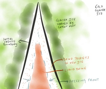
In this proposed basal crevassing mechanism, when a basal crevasse forms in ice that is colder than the freezing temperature of the brine, the brine immediately begins to freeze upon injection and contact with the cold ice. As brine freezes, the ice crystal growth process rejects salts and impurities – this process is known as cryoconcentration. Salt rejection during freezing leads to a plane of brine with higher salt concentration along the central axis of the crevasse (Fig. 10). As with sea ice formation, however, pockets of brine are trapped along crystal boundaries during freezing, creating a distribution of brine throughout the crevasse. The freezing process also generates latent heat, which is conducted away from the crevasse into the surrounding ice at a rate that depends on the thermal conductivity of the ambient ice (clean or debris-laden) and the temperature gradient (Fig. 10). Freezing continues until the brine and ambient ice reach thermal equilibrium, warming up to several meters of ice on either side in the process. Tulaczyk and others (in prep) measured ice temperatures that show evidence of this latent heat warming. Because warmer ice has a lower viscosity, this latent heat source also localizes strain in the glacier and induces multiple, repeated crevasse opening and brine injection events that help sustain the englacial pathway imaged by RES. Both the latent heat release and cryconcentration mechanisms occur subglacially as well as englacially and allow brine to remain liquid and move through this hydrologic system prior to final episodic subaerial release at Blood Falls, when a surface crevasse penetrates into the pressurized englacial brine zone (Carr and others, in prep).
6. CONCLUSION
Because ice temperatures, even at the bed, are well below the freezing point for freshwater (Hubbard and others, Reference Hubbard, Lawson, Anderson, Hubbard and Blatter2004; Pettit and others, Reference Pettit, Whorton, Waddington and Sletten2014), lower Taylor Glacier is not expected to sustain a thermally stable subglacial or englacial hydrologic system. To support such a hydrologic system, some combination of highly concentrated brine, to lower the freezing temperature and a local heat source, for example from latent heat of freezing or viscous strain heating, is necessary. We show that Taylor Glacier hosts this type of hydrologic system that feeds the brine outflow feature called Blood Falls.
This study has several key findings that are specific to understanding the hydrologic system feeding Blood Falls and several key findings that are important beyond Taylor Glacier. With respect to Taylor Glacier and Blood Falls, we find that:
(1) An elongated englacial zone of brine existing within the ice at mid depth is found by imaging the glacier ice within 300 m upstream of Blood Falls using RES (Fig. 5). Based on our upstream RES data, the zone outlined in Fig. 5 may be the confluence of two or more branches of englacial brine pathways.
(2) Given our assumptions, the liquid brine content increases from nil outside the scattering zone to >13% within 2 m of the central axis (Fig. 6). Scattering of the electromagnetic-wave signal, however, precludes measurement of the maximum brine content directly along the central axis of the englacial zone. The liquid brine content along this central axis may reach 100% because the freezing process slows as the brine and surrounding glacial ice reach a thermal equilibrium.
(3) The artesian character of the Blood Falls system is due to localized subglacial channeling, trapping, and pressurizing of brine. In particular, subglacial hydraulic-potential and hydraulic-pathways modeling show that supraglacial valleys, which have relief up to 50% of the ice thickness, split the subglacial water flow such that flow along the northern side of the glacier is directed and trapped by ice-cored moraines near Blood Falls, while flow along the middle and southern side of the glacier flows subglacially and continuously into Lake Bonney (Figs 8 and 9).
(4) Our results support the conceptual model proposed by Carr and others (in prep), that Blood Falls acts as a ‘pressure-release valve’ for the hydrologic system. Subglacial brine pools and is pressurized upstream from Blood Falls; it is injected englacially by basal crevassing where it can remain liquid due to cryoconcentration and latent heat release; it is advected towards the terminus by ice flow; and ultimately is released as an episodic artesian well through connection with surface crevassing events.
While Blood Falls is thought to be a unique system, it is better described as a member within a spectrum of possible hydrologic systems and it provides insight into glacial hydrology more broadly. From this study, our results suggest two important concepts that contribute to our understanding of subglacial and englacial hydrologic systems in any glacier:
(1) High-relief supraglacial topography can drive pathways of subglacial liquid flow. While this concept is a direct result of the hydraulic potential modeling and thus is not new, we show that it can play a significant role in the development and evolution of a subglacial hydrologic system.
(2) Latent heat of freezing alone may be sufficient to locally warm glacier ice and sustain freshwater hydrologic systems in other cold glaciers. Though freezing-point depression due to salinity is a significant factor for keeping the brine in a liquid state at Taylor Glacier, the measured temperature difference between the glacier ice (−17°C) and the brine freezing temperature (−7°C) is nearly 10°C (Pettit, in prep; personal communication EnEx-IceMole Team). Additional cryoconcentration may be able to locally reduce this difference, but latent heat significantly affects the thermal equilibrium (as shown by Tulaczyk and others, in prep). We predict, then, that a cold glacier with an average ice temperature of −8°C to −10°C may be able to sustain a freshwater hydrologic system.
ACKNOWLEDGEMENTS
This work was funded by the US National Science Foundation Division of Polar Programs with grants to E.C.P. (1144177), S.T. (1144192), J.A.M. (1619795), and W.B.L (1144176). Some preliminary data and ideas stemmed from observations made by E.C.P in 2004–06 supported by NSF-PLR grants to B. Hallet (0230338) and A. Fountain (0233823). Some of this material is based on data and equipment services provided by the UNAVCO Facility with support from the National Science Foundation (NSF) under NSF Cooperative Agreement No. EAR-0735156, 1255679, 1053220. The US NSF additionally awarded a Research Experience for Undergraduates Fellowship to J.A.B. through the University of Alaska Fairbanks. C.G.C. was funded by the S.T. Lee Young Research Travel Award to process the GPS data at the Antarctic Research Centre, Victoria University of Wellington. Colorado College provided the facilities and ESRI ArcGIS software for some of the data analysis. J.A.B. was originally inspired to study glaciers through the Girls on Ice program founded by E.C.P. E.C.P., S.T., J.A.M., and W.B.L. conceived the project and developed the field plan. E.C.P. supervised the project. E.C.P., C.G.C., and J.A.B. conducted the fieldwork and processed the data under E.C.P.’s supervision. Cecelia Mortenson provided mountaineering support during data collection. All authors contributed to development of the analyses, interpretation of the results, and extensive manuscript editing. The MIDGE Science team provided further support and input; the MIDGE Science team includes: Jill Mikucki, Erin Pettit, Slawek Tulaczyk, Bernd Dachwald, W. Berry Lyons, Jessica Badgeley, Richard Campen, Christina Carr, Michelle Chua, Ryan Davis, Ilya Digel, Clemens Espe, Marco Feldmann, Gero Francke, Neil Foley, Tiffany Green, Dirk Heinen, Julia Kowalski, Matthew Tuttle, Jacob Walter, and Kathleen Welch. This work was conducted in cooperation with Enceladus Explorer (EnEx) project (PI Bernd Dachwald). The EnEx project (grants 50NA1206 to 50NA1211) is funded by the DLR Space Administration.

 Open access