


1 Introduction
An active area of research focuses on identifying minimal size conditions on a set that ensure it contains a similar copy of a given finite point configuration. Size may refer to positive upper density, positive Lebesgue measure, sufficient Hausdorff dimension, or to some other notion of magnitude. Finite point configurations include arithmetic progressions, simplexes, chains, trees, and more general graphs.
In this article, we focus on the occurrence of arithmetic progressions and triangles in compact subsets of
 $\mathbb {R}^d$
for
$\mathbb {R}^d$
for
 $d\geq 1$
. We say that a point configuration
$d\geq 1$
. We say that a point configuration
 $P=(v^i)_{i=1}^k$
is realized in a set A if A contains a similar copy of P. Further, we say that P is stably realized in A if the set of t for which A contains a rotated and translated copy of
$P=(v^i)_{i=1}^k$
is realized in a set A if A contains a similar copy of P. Further, we say that P is stably realized in A if the set of t for which A contains a rotated and translated copy of
 $tP$
has nonempty interior.
$tP$
has nonempty interior.
Arithmetic progressions have been investigated in a variety of context. Szemerédi [Reference Szemerédi37] famously showed that any subset of the natural numbers with positive upper density contains arbitrarily long arithmetic progressions. A higher-dimensional variant was first obtained by Furstenberg and Katznelson [Reference Furstenberg and Katznelson12]; see also [Reference Bourgain6, Reference Lyall and Magyar25, Reference Ziegler43] for further developments.
In another direction, it is a consequence of the Lebesgue density theorem that any finite point configuration is stably realized in any subset of
 $\mathbb {R}^d$
of positive Lebesgue measure. In particular, arithmetic progressions of arbitrary finite length are stably realized in sets of positive measure. One must exercise some caution though. Bourgain [Reference Bourgain6] showed that any subset of
$\mathbb {R}^d$
of positive Lebesgue measure. In particular, arithmetic progressions of arbitrary finite length are stably realized in sets of positive measure. One must exercise some caution though. Bourgain [Reference Bourgain6] showed that any subset of
 $\mathbb {R}^3$
with positive upper density contains the vertices of an equilateral triangle, as well as all sufficiently large scalings. This result, however, does apply to sufficiently large scalings of arithmetic progressions (see a counter example in [Reference Bourgain6, Example b]).
$\mathbb {R}^3$
with positive upper density contains the vertices of an equilateral triangle, as well as all sufficiently large scalings. This result, however, does apply to sufficiently large scalings of arithmetic progressions (see a counter example in [Reference Bourgain6, Example b]).
A topological variant, provided by the second listed author and Mcdonald [Reference McDonald and Taylor30], states that if B is a second category Baire space in
 $\mathbb {R}^d$
(or in any topological vector space V), and
$\mathbb {R}^d$
(or in any topological vector space V), and
 $P \subset V$
is a countable bounded sequence, then P is stably realized in B. In particular, B contains arbitrarily long arithmetic progressions and all sufficiently small scalings.
$P \subset V$
is a countable bounded sequence, then P is stably realized in B. In particular, B contains arbitrarily long arithmetic progressions and all sufficiently small scalings.
A finer notion of size, Hausdorff dimension, is central in harmonic analysis and geometric measure theory. The celebrated Falconer distance problems ask how large the Hausdorff dimension of a compact set
 $E\subset \mathbb {R}^d$
,
$E\subset \mathbb {R}^d$
,
 $d\geq 2$
, needs to be to guarantee that its distance set
$d\geq 2$
, needs to be to guarantee that its distance set
 $$ \begin{align*}\Delta(E) = \{|x-y|:x,y\in E\}\end{align*} $$
has positive Lebesgue measure. Falconer demonstrated that
 $\dim _{\mathrm {H}}(E)>\frac {d}{2}$
is necessary and
$\dim _{\mathrm {H}}(E)>\frac {d}{2}$
is necessary and
 $\dim _{\mathrm { H}}(E)>\frac {d+1}{2}$
suffices [Reference Falconer9]; for more recent developments, see the introduction and references in [Reference Borges, Foster, Ou and Palsson5]. Resolving this gap – namely, establishing that the threshold
$\dim _{\mathrm { H}}(E)>\frac {d+1}{2}$
suffices [Reference Falconer9]; for more recent developments, see the introduction and references in [Reference Borges, Foster, Ou and Palsson5]. Resolving this gap – namely, establishing that the threshold
 $\frac {d}{2}$
suffices in Falconer’s conjecture – is a major open problem in harmonic analysis and geometric measure theory.
$\frac {d}{2}$
suffices in Falconer’s conjecture – is a major open problem in harmonic analysis and geometric measure theory.
Hausdorff dimension has further been used by a number of authors in analyzing the occurrence and abundance of finite point configurations. This includes, for instance, results on the interior of distance sets associated to chains [Reference Bennett, Iosevich and Taylor2], trees [Reference Borges, Foster, Ou and Palsson5, Reference Greenleaf, Iosevich and Taylor17, Reference Iosevich and Taylor19], necklaces [Reference Greenleaf, Iosevich and Pramanik15], and triangles [Reference Greenleaf, Iosevich and Taylor16, Reference Palsson and Acosta34]; results on the Lebesgue measure of distance sets associated to chains [Reference Ou and Taylor32] and triangles [Reference Greenleaf and Iosevich14]; conditions for the occurrence of equilateral triangles in
 $\mathbb {R}^3$
[Reference Iosevich and Magyar20] and the occurrence of arithmetic progressions (with additional assumptions involving Fourier dimension and supported measures) [Reference Chan, Łaba and Pramanik8].
$\mathbb {R}^3$
[Reference Iosevich and Magyar20] and the occurrence of arithmetic progressions (with additional assumptions involving Fourier dimension and supported measures) [Reference Chan, Łaba and Pramanik8].
Hausdorff dimension alone, however, is not enough to guarantee the existence of arithmetic progressions in subsets of
 $\mathbb {R}^d$
. Keleti [Reference Keleti23] showed that given any distinct set
$\mathbb {R}^d$
. Keleti [Reference Keleti23] showed that given any distinct set
 $\{x,y,z\}\subset \mathbb {R}$
there exists a compact set in
$\{x,y,z\}\subset \mathbb {R}$
there exists a compact set in
 $\mathbb {R}$
of Hausdorff dimension
$\mathbb {R}$
of Hausdorff dimension
 $1$
which does not contain any similar copy of
$1$
which does not contain any similar copy of
 $\{x,y,z\}$
. Máthé demonstrated that full Hausdorff dimension is not enough in any dimension to guarantee the occurrence of
$\{x,y,z\}$
. Máthé demonstrated that full Hausdorff dimension is not enough in any dimension to guarantee the occurrence of
 $3$
-point arithmetic progressions (this follows from considering the zeros of the polynomial
$3$
-point arithmetic progressions (this follows from considering the zeros of the polynomial
 $P(x_1,x_2,x_3)= x_1-2x_2+x_3$
in Theorem 2.3 of [Reference Máthé27]). Hence, even if a set has full Hausdorff dimension, it may not contain a
$P(x_1,x_2,x_3)= x_1-2x_2+x_3$
in Theorem 2.3 of [Reference Máthé27]). Hence, even if a set has full Hausdorff dimension, it may not contain a
 $3$
-term arithmetic progressions.
$3$
-term arithmetic progressions.
Another important 3-point configuration is a triangle. Depending on the ambient dimension, Hausdorff dimension is sometimes enough to guarantee the realization of similar triangles. Given any
 $3$
-point set, constructions due to Falconer [Reference Falconer10] and Maga [Reference Maga26] show that there exists a set of full Hausdorff dimension in the plane that does not contain any similar copy. The situation is better, however, for triangles in Legesbue null sets in dimension three. Iosevich and Magyar [Reference Iosevich and Magyar20] prove that there exists a dimensional threshold
$3$
-point set, constructions due to Falconer [Reference Falconer10] and Maga [Reference Maga26] show that there exists a set of full Hausdorff dimension in the plane that does not contain any similar copy. The situation is better, however, for triangles in Legesbue null sets in dimension three. Iosevich and Magyar [Reference Iosevich and Magyar20] prove that there exists a dimensional threshold
 $s< 3$
so that if
$s< 3$
so that if
 $E\subset \mathbb {R}^3$
with
$E\subset \mathbb {R}^3$
with
 $\dim _H(E)>s$
, then E contains the vertices of a simplex V for any non-degenerate
$\dim _H(E)>s$
, then E contains the vertices of a simplex V for any non-degenerate
 $3$
-simplex V satisfying a volume condition. They also prove a more general result for k-simplices. Note the non-degeneracy assumption precludes arithmetic progressions.
$3$
-simplex V satisfying a volume condition. They also prove a more general result for k-simplices. Note the non-degeneracy assumption precludes arithmetic progressions.
One might hope that Hausdorff dimension combined with some other conditions on structure or size may be enough to guarantee the occurrence of arithmetic progressions. Łaba and Pramanik [Reference Łaba and Pramanik24] provide sufficient conditions based on Fourier decay and power mass decay for a closed set
 $E\subset \mathbb {R}$
to contain a nontrivial
$E\subset \mathbb {R}$
to contain a nontrivial
 $3$
-term arithmetic progression; see also [Reference Chan, Łaba and Pramanik8] for a generalization to higher dimensions and more general patterns. However, even sets in
$3$
-term arithmetic progression; see also [Reference Chan, Łaba and Pramanik8] for a generalization to higher dimensions and more general patterns. However, even sets in
 $\mathbb {R}$
with both maximal Fourier and Hausdorff dimension need not contain
$\mathbb {R}$
with both maximal Fourier and Hausdorff dimension need not contain
 $3$
-APs. Shmerkin [Reference Shmerkin35] demonstrated the dependence of the results in [Reference Łaba and Pramanik24] on the choice of constants by constructing Salem sets (sets of full Fourier dimension) that contain no arithmetic progressions.
$3$
-APs. Shmerkin [Reference Shmerkin35] demonstrated the dependence of the results in [Reference Łaba and Pramanik24] on the choice of constants by constructing Salem sets (sets of full Fourier dimension) that contain no arithmetic progressions.
The results of this section inform us that an alternative notion of size other than Hausdorff dimension is required to guarantee the existence arithmetic progressions in
 $\mathbb {R}^d$
, as well as triangles in the plane.
$\mathbb {R}^d$
, as well as triangles in the plane.
In contrast, the results of the current paper are exciting in that they provide new insights for
 $3$
-point configurations, including arithmetic progressions, in subsets of the plane (see Section 2). With this, we turn to Newhouse thickness.
$3$
-point configurations, including arithmetic progressions, in subsets of the plane (see Section 2). With this, we turn to Newhouse thickness.
1.1 Newhouse thickness
In the 1970s, Newhouse introduced a notion of size known as thickness for compact subsets of the real line. His clever Gap Lemma gives conditions based on thickness that guarantee that a pair of compact sets intersect. Newhouse’s original motivation was the study of bifurcation theory in dynamical systems [Reference Newhouse31]. Since then, thickness has been used extensively in the fields of dynamical systems and fractal geometry, and even in numerical problem solving [Reference Astels1, Reference Boone and Palsson4, Reference Hunt, Kan and Yorke18, Reference Jung and Lai21, Reference McDonald and Taylor29, Reference Simon and Taylor36, Reference Yavicoli38, Reference Yavicoli and Yu41, Reference Yu42], and higher-dimensional notions of thickness have been introduced [Reference Biebler3, Reference Falconer and Yavicoli11, Reference Yavicoli40].
Newhouse thickness is a natural notion of size for compact sets. The complement of every compact set C in
 $\mathbb {R}$
is a countable union of open intervals. Discarding the two unbounded open intervals, we are left with a countable union of bounded, open intervals which we call gaps
$\mathbb {R}$
is a countable union of open intervals. Discarding the two unbounded open intervals, we are left with a countable union of bounded, open intervals which we call gaps
 $(G_n)$
. Without loss of generality, order the gaps by nonincreasing size. We can then construct C by removing, in order, the gaps
$(G_n)$
. Without loss of generality, order the gaps by nonincreasing size. We can then construct C by removing, in order, the gaps
 $(G_n)$
from the convex hull of C, denoted by
$(G_n)$
from the convex hull of C, denoted by
 $\operatorname {\mathrm {conv}}(C)$
. Observe that every time a gap
$\operatorname {\mathrm {conv}}(C)$
. Observe that every time a gap
 $G_n$
is removed, two intervals, one to the left of the gap,
$G_n$
is removed, two intervals, one to the left of the gap,
 $L_n$
, and one to the right of the gap,
$L_n$
, and one to the right of the gap,
 $R_n$
(we call these bridges). Newhouse thickness is computed by considering the ratios of the lengths of the bridges to the lengths of the gaps [Reference Newhouse31, Reference Yavicoli38].
$R_n$
(we call these bridges). Newhouse thickness is computed by considering the ratios of the lengths of the bridges to the lengths of the gaps [Reference Newhouse31, Reference Yavicoli38].
Definition 1.1 Let
 $C\subset \mathbb {R}$
be a compact set with convex hull I, and let
$C\subset \mathbb {R}$
be a compact set with convex hull I, and let
 $(G_n)$
be the open intervals making up
$(G_n)$
be the open intervals making up
 $I\setminus C$
, ordered in decreasing length. Each gap
$I\setminus C$
, ordered in decreasing length. Each gap
 $G_n$
is removed from a closed interval
$G_n$
is removed from a closed interval
 $I_n$
, leaving behind two closed intervals
$I_n$
, leaving behind two closed intervals
 $L_n$
and
$L_n$
and
 $R_n$
; the left and right pieces of
$R_n$
; the left and right pieces of
 $I_n\setminus G_n$
. The Newhouse thickness of C is defined by
$I_n\setminus G_n$
. The Newhouse thickness of C is defined by
 $$ \begin{align*} \tau\left( C\right):= \inf_{n\in\mathbb{N}} \frac{\min\left\{|L_n|,|R_n|\right\}}{|G_n|}. \end{align*} $$
Example (A classic set with thickness 1) The middle-third Cantor set has thickness equal to
 $1$
. This set is constructed by removing the middle-third of the interval
$1$
. This set is constructed by removing the middle-third of the interval
 $|G_n|=\frac {1}{3^n}$
. At each stage, this process leaves left and right intervals of length
$|G_n|=\frac {1}{3^n}$
. At each stage, this process leaves left and right intervals of length
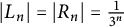 $|L_n|=|R_n|=\frac {1}{3^n}$
.
$|L_n|=|R_n|=\frac {1}{3^n}$
.
The key fact on which the results of this article are based is that sets of sufficient Newhouse thickness contain arithmetic progressions. The following is from [Reference Yavicoli39, Proposition 20].
Proposition 1.1 (Yavicoli [Reference Yavicoli39])
Let
 $C\subset \mathbb {R}$
be a compact set with
$C\subset \mathbb {R}$
be a compact set with
 $\tau (C)\geq 1$
. Then, C contains an arithmetic progression of length
$\tau (C)\geq 1$
. Then, C contains an arithmetic progression of length
 $3$
.
$3$
.
This result says that compact subsets of the real line with thickness at least 1 contain a
 $3$
-point arithmetic progression. Note that larger thickness is required for longer progressions (see Remarks 2.6 and 2.7).
$3$
-point arithmetic progression. Note that larger thickness is required for longer progressions (see Remarks 2.6 and 2.7).
We generalize Proposition 1.1 and provide an analog in higher dimensions. The main results of this article are as follows; we:
-
(1) prove a more general version of Proposition 1.1 for convex combinations in
 $\mathbb {R}$
(Proposition 2.1);
$\mathbb {R}$
(Proposition 2.1); -
(2) apply this to obtain similar copies of any triangle in Cartesian products in
$\mathbb {R}^2$
(Theorem 2.2); -
(3) prove a higher-dimensional analog that demonstrates the occurrence of arithmetic progressions and convex combinations in compact subsets of
$\mathbb {R}^d$
(Theorem 2.8); -
(4) obtain similar copies of any triangle in general compact sets in
$\mathbb {R}^d$
(Theorem 2.12).


1.2 The Gap Lemma
The main tool used to prove Proposition 1.1 is the Gap Lemma, which gives criteria for the intersection of two compact sets. Note that (ii) implies (i), but we list (i) for emphasis.
Lemma 1.2 (Newhouse’s Gap Lemma [Reference Newhouse31])
Let
 $C^1$
and
$C^1$
and
 $C^2$
be two compact sets in the real line such that:
$C^2$
be two compact sets in the real line such that:
-
(1)
$\operatorname {\mathrm {conv}}(C^1)\cap \operatorname {\mathrm {conv}}(C^2)\neq \emptyset $
; -
(2) neither set lies in a gap of the other set;
-
(3)
$\tau (C^1)\tau (C^2)\geq 1$
.
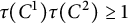
Then,
 $$ \begin{align*} C^1\cap C^2\neq \emptyset. \end{align*} $$
The Gap Lemma is useful in the study of patterns as patterns and intersections are directly connected. A set
 $E\subset \mathbb {R}^d$
contains a homothetic copy of a
$E\subset \mathbb {R}^d$
contains a homothetic copy of a
 $P=\{v^i\}_{i=1}^k$
if and only if there exists
$P=\{v^i\}_{i=1}^k$
if and only if there exists
 $t\neq 0$
so that
$t\neq 0$
so that
 $$ \begin{align*}\bigcap_{i=1}^k \left( E- tv^i\right) \neq \emptyset.\end{align*} $$
The Gap Lemma has played a role in the investigation of finite point configurations in a number of prior works. Simon and Taylor [Reference Simon and Taylor36] considered Cantor sets
 $K_1,K_2\subset \mathbb {R}$
satisfying
$K_1,K_2\subset \mathbb {R}$
satisfying
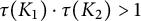 $\tau (K_1)\cdot \tau (K_2)>1$
, and showed that for any
$\tau (K_1)\cdot \tau (K_2)>1$
, and showed that for any
 $x\in \mathbb {R}^2$
, the pinned distance set
$x\in \mathbb {R}^2$
, the pinned distance set
 $$ \begin{align*} \Delta_x(K_1\times K_2) := \left\{|x-y| : y\in K_1\times K_2\right\} \end{align*} $$
has non-empty interior. This work was later extended by McDonald and Taylor in [Reference McDonald and Taylor28] where they proved that the distance set of a tree T of
 $K_1\times K_2$
, defined by
$K_1\times K_2$
, defined by
 $$ \begin{align*} \Delta_T(K_1\times K_2) = \left\{ ( |y^i-y^j|)_{i\sim j} : y^1,\ldots, y^{k+1}\in K_1\times K_2, y^i\neq y^j\right\}, \end{align*} $$
has non-empty interior, where a tree is a finite acyclic graph. They continued this work in [Reference McDonald and Taylor29], where infinite trees and constant gap trees were investigated.
Progress has been made toward developing and applying higher-dimensional gap lemmas. Boone and Palsson [Reference Boone and Palsson4] obtain higher-dimensional chain results for thick set using a higher-dimensional notion of thickness introduced by Falconer and Yavicoli. Jung and Taylor [Reference Jung and Taylor22] investigate chains and trees using the containment lemma (which serves as a substitute to the gap lemma) and the distance set results introduced in [Reference Jung and Lai21].
Yavicoli proved that compact sets in
 $\mathbb {R}^d$
generated by a restricted system of balls with significantly large thickness contain homothetic copies of finite sets [Reference Yavicoli40]. The current article offers an improvement to Yavicoli’s result for the specific setting of 3-point configurations by lowering the thickness threshold.
$\mathbb {R}^d$
generated by a restricted system of balls with significantly large thickness contain homothetic copies of finite sets [Reference Yavicoli40]. The current article offers an improvement to Yavicoli’s result for the specific setting of 3-point configurations by lowering the thickness threshold.
2 Main results
We investigate 3-point configurations in both
 $\mathbb {R}$
and in
$\mathbb {R}$
and in
 $\mathbb {R}^d$
. Our first main results concern 3-point configurations on the real line. As an application, we demonstrate the existence of similar copies of any triangle in sets of the form
$\mathbb {R}^d$
. Our first main results concern 3-point configurations on the real line. As an application, we demonstrate the existence of similar copies of any triangle in sets of the form
 $C\times C$
when
$C\times C$
when
 $C\subset \mathbb {R}$
is compact and
$C\subset \mathbb {R}$
is compact and
 $\tau (C)\geq 1.$
These results appear in Section 2.1 and rely on the Newhouse gap lemma as a primary tool.
$\tau (C)\geq 1.$
These results appear in Section 2.1 and rely on the Newhouse gap lemma as a primary tool.
Our second main results concern the existence of arithmetic progressions and any other 3-point configuration in compact subsets of
 $\mathbb {R}^d$
, including equilateral triangles. These results appear in Section 2.2 and rely on Yavicoli’s notion of thickness.
$\mathbb {R}^d$
, including equilateral triangles. These results appear in Section 2.2 and rely on Yavicoli’s notion of thickness.
2.1 3-Point configurations in
$\mathbb {R}$
& triangles in the plane part I

First, we demonstrate the following more general version of Proposition 1.1, which recovers the original result when
 $\lambda =\frac {1}{2}$
.
$\lambda =\frac {1}{2}$
.
Proposition 2.1 (Convex combinations in
$\mathbb {R}$
)

Let
 $C\subset \mathbb {R}$
be a compact set with
$C\subset \mathbb {R}$
be a compact set with
 ${\tau (C)\geq 1}$
. Then, for each
${\tau (C)\geq 1}$
. Then, for each
 $\lambda \in (0, 1)$
, the set C contains a nondegenerate
$\lambda \in (0, 1)$
, the set C contains a nondegenerate
 $3$
-term progression of the form
$3$
-term progression of the form
 $$ \begin{align*}\{a, (1-\lambda)a + \lambda b , b\}.\end{align*} $$
In other words, any 3-point subset of the line is realized in C.
The proof of this result relies on demonstrating that
 $C\cap \left ( (1-\lambda ) C+ \lambda C \right )\neq \emptyset $
and is found in Section 4.
$C\cap \left ( (1-\lambda ) C+ \lambda C \right )\neq \emptyset $
and is found in Section 4.
As a consequence of Proposition 2.1 combined with the fact that the interior of the difference set
 $$ \begin{align*}C-C= \{x-y: x,y\in C\}\end{align*} $$
has non-empty interior, we have the following geometric consequence for triangles.
Theorem 2.2 (3-point configurations in
$C\times C$
)

Let T denote any 3-point set in
 $\mathbb {R}^2$
. If
$\mathbb {R}^2$
. If
 $\tau (C) \geq 1$
, then
$\tau (C) \geq 1$
, then
 $C\times C$
contains a similar copy of T.
$C\times C$
contains a similar copy of T.
It follows from Theorem 2.2 that the Cartesian product
 $C\times C$
contains the vertices of a similar copy of any 3-point configuration whenever
$C\times C$
contains the vertices of a similar copy of any 3-point configuration whenever
 $C \subset \mathbb {R}$
is a compact set satisfying
$C \subset \mathbb {R}$
is a compact set satisfying
 $\tau (C) \geq 1$
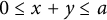
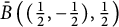
. For emphasis, we state the result for equilateral triangles (see Figure 1).
$\tau (C) \geq 1$
. For emphasis, we state the result for equilateral triangles (see Figure 1).
We see that
 $C\times C$
contains an equilateral triangle by combining two facts: (i) C contains an arithmetic progression
$C\times C$
contains an equilateral triangle by combining two facts: (i) C contains an arithmetic progression
 $\mathcal {A} = \{x, x+t, x+2t\}$
, where
$\mathcal {A} = \{x, x+t, x+2t\}$
, where
 $t>0$
can be taken arbitrarily small; (ii) the distance set
$t>0$
can be taken arbitrarily small; (ii) the distance set
 $\Delta (C)$
contains an interval
$\Delta (C)$
contains an interval
 $[0,\ell ]$
for some
$[0,\ell ]$
for some
 $\ell>0$
.
$\ell>0$
.

Corollary 2.3 If
 $\tau (C) \geq 1$
, then
$\tau (C) \geq 1$
, then
 $C\times C$
contains the vertices of an equilateral triangle.
$C\times C$
contains the vertices of an equilateral triangle.
The proofs for the results in this section appear in Section 4.
Remark 2.4 (Our result is a first of its kind in
$\mathbb {R}^2$
)

Our Theorem 2.2 (and Theorem 2.12 below) are among the first in the literature to give explicit criteria for the occurrence of 3-point configurations in the plane, following the work of Chan–Łaba–Pramanik [Reference Chan, Łaba and Pramanik8] proving the existence of
 $3$
-term arithmetic progressions in some closed subsets of
$3$
-term arithmetic progressions in some closed subsets of
 $\mathbb {R}^d$
with sufficient Fourier decay and power mass decay, respectively, and Yavicoli [Reference Yavicoli40] showing that subsets of
$\mathbb {R}^d$
with sufficient Fourier decay and power mass decay, respectively, and Yavicoli [Reference Yavicoli40] showing that subsets of
 $\mathbb {R}^d$
of Yavicoli-thickness larger than
$\mathbb {R}^d$
of Yavicoli-thickness larger than
 $10^7$
contain
$10^7$
contain
 $3$
-point configurations.
$3$
-point configurations.
Remark 2.5 (Comparison between Newhouse thickness and Hausdorff dimension)
As mentioned above, Hausdorff dimension alone is not enough to guarantee the realization of similar triangles in subsets of
 $\mathbb {R}^2$
. Our result gives a class of compact Lebesgue null subsets of
$\mathbb {R}^2$
. Our result gives a class of compact Lebesgue null subsets of
 $\mathbb {R}^2$
and explicit criteria, mainly
$\mathbb {R}^2$
and explicit criteria, mainly
 $\tau (C)\geq 1$
, that guarantees the realization of a similar copy of any 3-point configuration in
$\tau (C)\geq 1$
, that guarantees the realization of a similar copy of any 3-point configuration in
 $C\times C$
. Because Hausdorff dimension and Newhouse thickness obey the following relationship [Reference Palis and Takens33] for
$C\times C$
. Because Hausdorff dimension and Newhouse thickness obey the following relationship [Reference Palis and Takens33] for
 $\tau (C)>0$
,
$\tau (C)>0$
,
 $$ \begin{align*} \dim_H(C) \geq \frac{\log(2)}{\log(2+\frac{1}{\tau(C)})}, \end{align*} $$
we can calculate a lower bound for the Hausdorff dimension of
 $C\times C$
using its thickness; i.e., since
$C\times C$
using its thickness; i.e., since
 $\tau (C)\geq 1$
, we know
$\tau (C)\geq 1$
, we know
 $\dim _H(C\times C)\geq 2\dim _H(C) \geq 2\frac {\log {2}}{\log {3}}$
.
$\dim _H(C\times C)\geq 2\dim _H(C) \geq 2\frac {\log {2}}{\log {3}}$
.
Remark 2.6 (Longer progressions)
For longer progressions, higher thickness is required. It is known that the middle-
 $\epsilon $
Cantor set
$\epsilon $
Cantor set
 $C_\epsilon $
does not contain arithmetic progressions of length
$C_\epsilon $
does not contain arithmetic progressions of length
 $\lfloor \frac {1}{\epsilon }\rfloor +2$
or larger. In particular, Broderick, Fishman, and Simmons [Reference Broderick, Fishman and Simmons7] proved that if
$\lfloor \frac {1}{\epsilon }\rfloor +2$
or larger. In particular, Broderick, Fishman, and Simmons [Reference Broderick, Fishman and Simmons7] proved that if
 $L_{\text {AP}}(S)$
denotes the maximal length of an arithmetic progression in a set
$L_{\text {AP}}(S)$
denotes the maximal length of an arithmetic progression in a set
 $S\subset \mathbb {R}$
, then for all
$S\subset \mathbb {R}$
, then for all
 $\epsilon>0$
sufficiently small and
$\epsilon>0$
sufficiently small and
 $n\in \mathbb {N}$
sufficiently large,
$n\in \mathbb {N}$
sufficiently large,
 $$ \begin{align*} L_{\text{AP}}(C_\epsilon)\leq 1/\epsilon + 1. \end{align*} $$
It is also not hard to see that
 $L_{\text {AP}}(C_\epsilon ) =2 $
for all
$L_{\text {AP}}(C_\epsilon ) =2 $
for all
 $\epsilon>\frac{1}{3}$
.
$\epsilon>\frac{1}{3}$
.
Further, using Newhouse’s gap lemma and symmetry,
 $L_{\text {AP}}(C_\epsilon ) \geq 4$
for all
$L_{\text {AP}}(C_\epsilon ) \geq 4$
for all
 $0<\epsilon \le \frac{1}{3}$
(this lower bound is attributed to Shmerkin and pointed out in [Reference Broderick, Fishman and Simmons7, Footnote 4]). Indeed, it follows by the gap lemma that there exists a
$0<\epsilon \le \frac{1}{3}$
(this lower bound is attributed to Shmerkin and pointed out in [Reference Broderick, Fishman and Simmons7, Footnote 4]). Indeed, it follows by the gap lemma that there exists a
 $t \in (C_\epsilon -\frac 12) \cap \frac 13(C_\epsilon - \frac 12)\neq \emptyset $
, and so we have
$t \in (C_\epsilon -\frac 12) \cap \frac 13(C_\epsilon - \frac 12)\neq \emptyset $
, and so we have
 $c_1, c_2 \in C_\epsilon $
so that
$c_1, c_2 \in C_\epsilon $
so that
 $$ \begin{align*}c_1 =\frac12 +t \,\,\, \text{ and } \,\,\, c_2 = \frac12+3t.\end{align*} $$
By symmetry of
 $C_\epsilon $
about
$C_\epsilon $
about
 $\frac 12$
, we further have
$\frac 12$
, we further have
 $c_3, c_4 \in C_\epsilon $
so that
$c_3, c_4 \in C_\epsilon $
so that
 $$ \begin{align*}c_3 = \frac12-t \,\,\, \text{ and } \,\,\, c_4 = \frac12 -3t,\end{align*} $$
which yields the desired
 $4$
-AP.
$4$
-AP.
Remark 2.7 (Sharpness of our result: the off-center Cantor set has thickness 1 and no
$4$
-AP)

We now construct a set of thickness
 $1$
that contains no
$1$
that contains no
 $4$
-term arithmetic progressions. We call our construction the off-center Cantor set and denote it
$4$
-term arithmetic progressions. We call our construction the off-center Cantor set and denote it
 $C_a$
.
$C_a$
.
Let
 $0<a<\frac {1}{3}$
. We construct
$0<a<\frac {1}{3}$
. We construct
 $C_a$
iteratively, starting with
$C_a$
iteratively, starting with
 $[0,1]$
, by removing from each interval I an open interval of length
$[0,1]$
, by removing from each interval I an open interval of length
 $a|I|$
, call this open interval G. Then,
$a|I|$
, call this open interval G. Then,
 $I\setminus G$
is split into two closed intervals: the left interval L of length
$I\setminus G$
is split into two closed intervals: the left interval L of length
 $a|I|$
and the right interval R of length
$a|I|$
and the right interval R of length
 $(1-2a)|I|$
. Hence, we remove
$(1-2a)|I|$
. Hence, we remove
 $(a,2a)$
from
$(a,2a)$
from
 $[0,1]$
to obtain
$[0,1]$
to obtain
 $[0,a]\cup [2a,1]$
. From these intervals, we remove
$[0,a]\cup [2a,1]$
. From these intervals, we remove
 $(a^2,2a^2)$
and
$(a^2,2a^2)$
and
 $(3a-2a^2,4a-4a^2)$
to obtain
$(3a-2a^2,4a-4a^2)$
to obtain
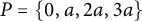
 $[0,a^2]\cup [2a^2,a]\cup [2a,3a-2a^2]\cup [4a-4a^2,1]$
, and so on, as illustrated in Figure 2.
$[0,a^2]\cup [2a^2,a]\cup [2a,3a-2a^2]\cup [4a-4a^2,1]$
, and so on, as illustrated in Figure 2.
First two iterations of off-center Cantor set
 $C_a$
for
$C_a$
for
 $a=\frac {3}{10}$
.
$a=\frac {3}{10}$
.

Observe that by construction
 $|L|=|G|< |R|$
; as this is true for every step in the construction of
$|L|=|G|< |R|$
; as this is true for every step in the construction of
 $C_a$
,
$C_a$
,
 $$ \begin{align*}\tau(C_a) =\frac{\min\{|L|,|R|\}}{|G|}=1.\end{align*} $$
Thus,
 $C_a$
is a self-similar set of thickness
$C_a$
is a self-similar set of thickness
 $1$
.
$1$
.
We will now show
 $C_a$
does not contain any
$C_a$
does not contain any
 $4$
-term arithmetic progressions for
$4$
-term arithmetic progressions for
 $\frac {2-\sqrt {2}}{2}<a<\frac {3-\sqrt {3}}{4}$
. Assume to the contrary that
$\frac {2-\sqrt {2}}{2}<a<\frac {3-\sqrt {3}}{4}$
. Assume to the contrary that
 $C_a$
contains a
$C_a$
contains a
 $4$
-AP, call it
$4$
-AP, call it
 $P=\{x,x+y,x+2y,x+3y\}$
. Then, there exists some smallest interval in the construction of
$P=\{x,x+y,x+2y,x+3y\}$
. Then, there exists some smallest interval in the construction of
 $C_a$
that contains P but P is split over two levels in the next step of the construction. Because of the self-similarity of
$C_a$
that contains P but P is split over two levels in the next step of the construction. Because of the self-similarity of
 $C_a$
, we assume without loss of generality that P is contained in
$C_a$
, we assume without loss of generality that P is contained in
 $[0,1]$
but splits over
$[0,1]$
but splits over
 $[0,a]\cup [2a,1]$
.
$[0,a]\cup [2a,1]$
.
For P to be contained in
 $[0,1]$
and split over
$[0,1]$
and split over
 $[0,a]\cup [2a,1]$
, we must have
$[0,a]\cup [2a,1]$
, we must have
 $0\leq x\leq a$
,
$0\leq x\leq a$
,
 $y\geq a$
(otherwise the arithmetic progression cannot jump the gap
$y\geq a$
(otherwise the arithmetic progression cannot jump the gap
 $(a,2a)$
), and
$(a,2a)$
), and
 $x+3y\leq 1$
. Then, observe that
$x+3y\leq 1$
. Then, observe that
 $x+y\ngeq 2a$
because if it was then
$x+y\ngeq 2a$
because if it was then
 $$ \begin{align*}x+3y\geq 2y+2a\geq 4a>1,\end{align*} $$
a contradiction. We also have
 $x+y\notin (a,2a)$
; otherwise, P would not be contained in
$x+y\notin (a,2a)$
; otherwise, P would not be contained in
 $C_a$
. Thus, it must be the case that
$C_a$
. Thus, it must be the case that
 $x+y\in [0,a]$
. Because
$x+y\in [0,a]$
. Because
 $0\leq x\leq a$
,
$0\leq x\leq a$
,
 $y\geq a$
, and
$y\geq a$
, and
 $0\leq x+y\leq a$
, we conclude that
$0\leq x+y\leq a$
, we conclude that
 $x=0$
and
$x=0$
and
 $y=a$
, so
$y=a$
, so
 $P=\{0,a,2a,3a\}$
.
$P=\{0,a,2a,3a\}$
.
Notice that
 $0,a,2a\in C_a$
, so it remains to show
$0,a,2a\in C_a$
, so it remains to show
 $3a\notin C_a$
. By construction of
$3a\notin C_a$
. By construction of
 $C_a$
, the interval
$C_a$
, the interval
 $[4a-4a^2,1]$
is split by the gap
$[4a-4a^2,1]$
is split by the gap
 $(5a-8a^2+4a^3,6a-12a^2+8a^3)$
, and by the assumption that
$(5a-8a^2+4a^3,6a-12a^2+8a^3)$
, and by the assumption that
 $\frac {2-\sqrt {2}}{2}<a<\frac {3-\sqrt {3}}{4}$
, we know
$\frac {2-\sqrt {2}}{2}<a<\frac {3-\sqrt {3}}{4}$
, we know
 $3a\in (5a-8a^2+4a^3,6a-12a^2+8a^3)$
. Consequently,
$3a\in (5a-8a^2+4a^3,6a-12a^2+8a^3)$
. Consequently,
 $C_a$
cannot contain P. By self-similarity,
$C_a$
cannot contain P. By self-similarity,
 $C_a$
cannot contain any
$C_a$
cannot contain any
 $4$
-term arithmetic progressions.
$4$
-term arithmetic progressions.
In the next section, we introduce higher-dimensional variants of Proposition 2.1 (on 3-point configurations on the line) and Theorem 2.2 (on triangles in the plane) that do not depend on Cartesian product structure.
2.2 3-Point configurations in
$\mathbb {R}^d$
& triangles in the plane part II

In this section, we introduce results in dimensions
 $d\geq 2$
. Theorem 2.8 of this section yields conditions to guarantee the occurrence of arithmetic progressions and other linear 3-point configurations in
$d\geq 2$
. Theorem 2.8 of this section yields conditions to guarantee the occurrence of arithmetic progressions and other linear 3-point configurations in
 $\mathbb {R}^d$
. Beyond linear combinations, Theorem 2.12 guarantees the occurrence of a similar copy of any 3-point configuration in higher dimensions.
$\mathbb {R}^d$
. Beyond linear combinations, Theorem 2.12 guarantees the occurrence of a similar copy of any 3-point configuration in higher dimensions.
Here, we use a higher-dimensional notion of thickness introduced by Yavicoli [Reference Yavicoli40]. We directly state the results of this section, and we delay formal introduction of Yavicoli thickness and the corresponding gap lemma to Section 3. We require the notion of a system of balls and r-uniformity, which will also be defined in Section 3.
Our first result says that a compact set C generated by a system of balls
 $\{S_I\}_I$
in
$\{S_I\}_I$
in
 $\mathbb {R}^d$
with Yavicoli thickness (Definition 3.2 below) satisfying
$\mathbb {R}^d$
with Yavicoli thickness (Definition 3.2 below) satisfying
 $$ \begin{align*} \tau\left( C,\{S_I\}\right) \geq \frac{2}{1-2r} \end{align*} $$
for some
 $0<r<\frac {1}{2}$
contains a
$0<r<\frac {1}{2}$
contains a
 $3$
-point arithmetic progression; e.g., any
$3$
-point arithmetic progression; e.g., any
 $\frac {1}{4}$
-uniformly compact set of thickness greater than
$\frac {1}{4}$
-uniformly compact set of thickness greater than
 $4$
contains an arithmetic progression of length
$4$
contains an arithmetic progression of length
 $3$
.
$3$
.
The proof of this result is inspired by the proof of Proposition 1.1. For a compact set C, we take two disjoint subsets A and B and apply the Gap Lemma to show that
 $C\cap \left (\lambda A +(1-\lambda )B\right ) \neq \emptyset $
. The assumption that
$C\cap \left (\lambda A +(1-\lambda )B\right ) \neq \emptyset $
. The assumption that
 $0<r< \frac{1}{2}$
is used to apply the gap lemma in Theorem 3.2. Our proofs quickly diverge, though, as we lose the well-ordering of
$0<r< \frac{1}{2}$
is used to apply the gap lemma in Theorem 3.2. Our proofs quickly diverge, though, as we lose the well-ordering of
 $\mathbb {R}$
in higher dimensions and the higher-dimensional Gap Lemma has a number of additional assumptions to verify over the one-dimensional Gap Lemma.
$\mathbb {R}$
in higher dimensions and the higher-dimensional Gap Lemma has a number of additional assumptions to verify over the one-dimensional Gap Lemma.
In particular, our method views compact sets in
 $\mathbb {R}^d$
as a sequence of nested balls, each generation of which is finite, and our method requires the existence of two first-generation children, call them
$\mathbb {R}^d$
as a sequence of nested balls, each generation of which is finite, and our method requires the existence of two first-generation children, call them
 $S_{1_A}$
and
$S_{1_A}$
and
 $S_{1_B}$
, out of the total
$S_{1_B}$
, out of the total
 $k_\emptyset $
first-generation children that are both disjoint from all first-generation children; these first-generation children
$k_\emptyset $
first-generation children that are both disjoint from all first-generation children; these first-generation children
 $S_{1_A}$
and
$S_{1_A}$
and
 $S_{1_B}$
are used to construct the sets A, B mentioned above. This requirement is explained in Section 3.1.
$S_{1_B}$
are used to construct the sets A, B mentioned above. This requirement is explained in Section 3.1.
Theorem 2.8 (Convex combinations in
$\mathbb {R}^d$
)

Let C be a compact set in
 $(\mathbb {R}^d,\operatorname {\mathrm {dist}})$
generated by the system of balls
$(\mathbb {R}^d,\operatorname {\mathrm {dist}})$
generated by the system of balls
 $\{S_I\}_I$
such that C is r-uniformly dense where
$\{S_I\}_I$
such that C is r-uniformly dense where
 $ 0<r<\frac {1}{2}$
. Let
$ 0<r<\frac {1}{2}$
. Let
 $\lambda \in (0,\frac 12]$
, and suppose that
$\lambda \in (0,\frac 12]$
, and suppose that
 $$ \begin{align*}\tau\left( C,\{S_I\}\right) \geq \frac{2(1-\lambda)}{\lambda(1-2r)}.\end{align*} $$
Suppose that there exist distinct first-generation children disjoint from all other children:
 $S_{1_A}$
and
$S_{1_A}$
and
 $S_{1_B}$
with
$S_{1_B}$
with
 $1\leq 1_A<1_B\leq k_\emptyset $
such that
$1\leq 1_A<1_B\leq k_\emptyset $
such that
 $S_{1_A} \cap S_i = \emptyset $
and
$S_{1_A} \cap S_i = \emptyset $
and
 $S_{1_B}\cap S_i =\emptyset $
for all
$S_{1_B}\cap S_i =\emptyset $
for all
 $i\neq 1_A,1_B$
where
$i\neq 1_A,1_B$
where
 $1\leq i\leq k_\emptyset $
. Then, C contains a
$1\leq i\leq k_\emptyset $
. Then, C contains a
 $3$
-point convex combination of the form
$3$
-point convex combination of the form
 $$ \begin{align*}\{a,\lambda a+(1-\lambda)b,b\}.\end{align*} $$
In particular, under the hypotheses above with
 $\lambda = \frac {1}{2}$
, we have the following.
$\lambda = \frac {1}{2}$
, we have the following.
Corollary 2.9 (
$3$
-term arithmetic progressions in
$\mathbb {R}^d$
)


Let C be a compact set in
 $(\mathbb {R}^d,\operatorname {\mathrm {dist}})$
generated by the system of balls
$(\mathbb {R}^d,\operatorname {\mathrm {dist}})$
generated by the system of balls
 $\{S_I\}_I$
such that C is r-uniformly dense, where
$\{S_I\}_I$
such that C is r-uniformly dense, where
 $ 0<r<\frac {1}{2}$
. Suppose that
$ 0<r<\frac {1}{2}$
. Suppose that
 $$ \begin{align*}\tau\left( C,\{S_I\}\right) \geq \frac{2}{1-2r},\end{align*} $$
and suppose that there exist distinct first-generation children of
 $\{S_I\}$
disjoint from all other children. Then, C contains an arithmetic progression
$\{S_I\}$
disjoint from all other children. Then, C contains an arithmetic progression
 $\{a, \frac {1}{2}(a+b),b\}$
with
$\{a, \frac {1}{2}(a+b),b\}$
with
 $a\neq b$
.
$a\neq b$
.
Remark 2.10 Observe Theorem 2.8 has a thickness condition that depends on r and
 $\lambda $
, whereas the one-dimensional analog, Proposition 2.1, does not. In the higher-dimensional Gap Lemma 3.2, there are additional assumptions such as r-uniformity and the relationships in (ii) and (iii) which ensure the sets are interwoven. These additional assumptions lead to a thickness condition that depends on r and
$\lambda $
, whereas the one-dimensional analog, Proposition 2.1, does not. In the higher-dimensional Gap Lemma 3.2, there are additional assumptions such as r-uniformity and the relationships in (ii) and (iii) which ensure the sets are interwoven. These additional assumptions lead to a thickness condition that depends on r and
 $\lambda $
.
$\lambda $
.
Next, we prove a result on the existence of triangles in compact sets of sufficient Yavicoli thickness, but first we need a way to categorize all triangles.
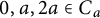
Definition 2.1 (Normalized triangle, Figure 3)
For
 $\alpha \geq 0$
,
$\alpha \geq 0$
,
 $\lambda \in (0,\frac 12]$
, we define
$\lambda \in (0,\frac 12]$
, we define
 $\mathcal {T}(\alpha ,\lambda )$
as the triangle consisting of the vertices
$\mathcal {T}(\alpha ,\lambda )$
as the triangle consisting of the vertices
 $\{x,y,z\}$
such that the angle at vertex z,
$\{x,y,z\}$
such that the angle at vertex z,
 $\theta _z$
, is the largest angle, and we normalize the longest side of the triangle, the side between vertices x and y, to be
$\theta _z$
, is the largest angle, and we normalize the longest side of the triangle, the side between vertices x and y, to be
 $1$
; i.e.,
$1$
; i.e.,
 $|y-x|=1$
. Let
$|y-x|=1$
. Let
 $\alpha $
denote the height of the triangle. The altitude from z bisects the line segment from x to y into two segments, and we denote their lengths by
$\alpha $
denote the height of the triangle. The altitude from z bisects the line segment from x to y into two segments, and we denote their lengths by
 $\lambda $
and
$\lambda $
and
 $(1-\lambda )$
.
$(1-\lambda )$
.
The triangle
 $T(\alpha ,\lambda )$
with vertices
$T(\alpha ,\lambda )$
with vertices
 $x,y,z$
, largest angle at z, height
$x,y,z$
, largest angle at z, height
 $\alpha $
, and base
$\alpha $
, and base
 $1$
.
$1$
.

Lemma 2.11 Let
 $\mathcal {T}$
be the vertices of any non-degenerate triangle in
$\mathcal {T}$
be the vertices of any non-degenerate triangle in
 $\mathbb {R}^2$
. Then, there exists an
$\mathbb {R}^2$
. Then, there exists an
 $(\alpha ,\lambda )$
in
$(\alpha ,\lambda )$
in
 $$ \begin{align*} \mathcal{R}= \left\{ (\alpha,\lambda)\in \mathbb{R}^2 : 0< \alpha , 0\leq \lambda \leq \frac{1}{2}, \alpha^2+(1-\lambda)^2\leq 1 \right\}, \end{align*} $$
such that
 $\mathcal {T}$
is similar to the triangle
$\mathcal {T}$
is similar to the triangle
 $\mathcal {T}(\alpha ,\lambda )$
.
$\mathcal {T}(\alpha ,\lambda )$
.
The lemma is immediate upon scaling, rotating, and labeling the vertices appropriately; the above inequalities are a simple consequence of the Pythagorean theorem.
Theorem 2.12 (Triangles in
$\mathbb {R}^2$
)

Let
 $\mathcal {T}$
denote the vertices of any triangle in
$\mathcal {T}$
denote the vertices of any triangle in
 $\mathbb {R}^2$
, and let
$\mathbb {R}^2$
, and let
 $\mathcal {T}(\alpha ,\lambda )$
be a triangle similar to
$\mathcal {T}(\alpha ,\lambda )$
be a triangle similar to
 $\mathcal {T}$
resulting from Lemma 2.11 for some
$\mathcal {T}$
resulting from Lemma 2.11 for some
 $\alpha $
,
$\alpha $
,
 $\lambda $
in
$\lambda $
in
 $\mathcal {R}$
. Let
$\mathcal {R}$
. Let
 $C\subset \mathbb {R}^2$
be a compact set generated by the system of balls
$C\subset \mathbb {R}^2$
be a compact set generated by the system of balls
 $\{S_I\}$
in the Euclidean norm such that C is r-uniformly dense for some
$\{S_I\}$
in the Euclidean norm such that C is r-uniformly dense for some
 $0<r<\frac {1}{2}$
. Suppose there exists distinct first-generation children
$0<r<\frac {1}{2}$
. Suppose there exists distinct first-generation children
 $S_{1_A}$
and
$S_{1_A}$
and
 $S_{1_B}$
,
$S_{1_B}$
,
 $1\leq 1_A<1_B\leq k_\emptyset $
, contained in
$1\leq 1_A<1_B\leq k_\emptyset $
, contained in
 $\bar {B}\left (0,\frac {1}{2}\right )$
such that
$\bar {B}\left (0,\frac {1}{2}\right )$
such that
 $S_{1_A}$
and
$S_{1_A}$
and
 $S_{1_B}$
are disjoint from all other first-generation children; i.e.,
$S_{1_B}$
are disjoint from all other first-generation children; i.e.,
 $S_{1_A}\cap S_i=\emptyset $
for all
$S_{1_A}\cap S_i=\emptyset $
for all
 $i\neq 1_A$
, and
$i\neq 1_A$
, and
 $S_{1_B}\cap S_i=\emptyset $
for all
$S_{1_B}\cap S_i=\emptyset $
for all
 $i\neq 1_B$
. Further, suppose
$i\neq 1_B$
. Further, suppose
 $$ \begin{align*}\tau\left( C,\{S_I\}\right) \geq \sqrt{\frac{\alpha^2+(1-\lambda)^2}{\alpha^2+\lambda^2}}\cdot \frac{2}{1-2r},\end{align*} $$
then C contains the vertices of a similar copy of
 $\mathcal {T}$
.
$\mathcal {T}$
.
In other words, given any 3-point set
 $\mathcal {T}$
, any set C satisfying the hypotheses contains a similar copy of
$\mathcal {T}$
, any set C satisfying the hypotheses contains a similar copy of
 $\mathcal {T}$
. A key tool in the proof is the higher gap lemma due to Yavicoli (see Theorem 3.2); the hypothesis that
$\mathcal {T}$
. A key tool in the proof is the higher gap lemma due to Yavicoli (see Theorem 3.2); the hypothesis that
 $r\in (0,\frac 12)$
is an assumption of the Gap lemma.
$r\in (0,\frac 12)$
is an assumption of the Gap lemma.
Remark 2.13 We suspect this holds in higher dimensions, but there are technical complexities that arise.
For equilateral triangles,
 $\lambda =\frac{1}{2}$
and
$\lambda =\frac{1}{2}$
and
 $\alpha = \frac {\sqrt {3}}{2}$
, and the thickness assumption is simplified so that we have the following.
$\alpha = \frac {\sqrt {3}}{2}$
, and the thickness assumption is simplified so that we have the following.
Corollary 2.14 (Equilateral triangles in
$\mathbb {R}^2$
)

Let
 $\mathcal {T}$
denote the vertices of an equilateral triangle. Let
$\mathcal {T}$
denote the vertices of an equilateral triangle. Let
 $C\subset \mathbb {R}^2$
be a compact set generated by the system of balls
$C\subset \mathbb {R}^2$
be a compact set generated by the system of balls
 $\{S_I\}$
in the Euclidean norm such that C is r-uniformly dense for some
$\{S_I\}$
in the Euclidean norm such that C is r-uniformly dense for some
 $0<r<\frac {1}{2}$
. Suppose there exists first-generation children
$0<r<\frac {1}{2}$
. Suppose there exists first-generation children
 $S_{1_A}$
and
$S_{1_A}$
and
 $S_{1_B}$
,
$S_{1_B}$
,
 $1\leq 1_A<1_B\leq k_\emptyset $
, contained in
$1\leq 1_A<1_B\leq k_\emptyset $
, contained in
 $\bar {B}\left (0,\frac {1}{2}\right )$
such that
$\bar {B}\left (0,\frac {1}{2}\right )$
such that
 $S_{1_A}$
and
$S_{1_A}$
and
 $S_{1_B}$
are disjoint from all other first-generation children. Further, suppose
$S_{1_B}$
are disjoint from all other first-generation children. Further, suppose
 $$ \begin{align*}\tau\left( C,\{S_I\}\right)\geq \frac{2}{1-2r},\end{align*} $$
then C contains the vertices of a similar copy of
 $\mathcal {T}$
.
$\mathcal {T}$
.
Remark 2.15 Above, we assume that
 $S_{1_A}$
,
$S_{1_A}$
,
 $S_{1_B}$
are contained in
$S_{1_B}$
are contained in
 $\bar {B}\left ( 0,\frac {1}{2}\right )$
, but this is not optimal. In the proof of Theorem 2.12, we will show that taking
$\bar {B}\left ( 0,\frac {1}{2}\right )$
, but this is not optimal. In the proof of Theorem 2.12, we will show that taking
 $S_{1_A}$
and
$S_{1_A}$
and
 $S_{1_B}$
in the larger ball,
$S_{1_B}$
in the larger ball,
 $\bar {B}\left ( 0, \frac {1}{2}+t_1-\frac {h_\emptyset (C) x}{2s_f}\right )$
, where the variables
$\bar {B}\left ( 0, \frac {1}{2}+t_1-\frac {h_\emptyset (C) x}{2s_f}\right )$
, where the variables
 $t_1, h_\emptyset (C)$
, and
$t_1, h_\emptyset (C)$
, and
 $s_f$
are defined in the proof, and
$s_f$
are defined in the proof, and
 $x=\max \left \{\frac {2r}{1-2r},0\right \}$
is sufficient.
$x=\max \left \{\frac {2r}{1-2r},0\right \}$
is sufficient.
Before, to guarantee the occurrence of a
 $3$
-AP, we needed
$3$
-AP, we needed
 $C\cap \left (\frac {A+B}{2}\right )\neq \emptyset $
for
$C\cap \left (\frac {A+B}{2}\right )\neq \emptyset $
for
 $A, B$
disjoint subsets of C. Now, to guarantee the occurrence of the vertices of an equilateral triangle, we need
$A, B$
disjoint subsets of C. Now, to guarantee the occurrence of the vertices of an equilateral triangle, we need
 $C\cap \left (H(A,B)\right )\neq \emptyset $
, where
$C\cap \left (H(A,B)\right )\neq \emptyset $
, where
 $H: \mathbb {R}^2\times \mathbb {R}^2 \rightarrow \mathbb {R}^2$
is defined by
$H: \mathbb {R}^2\times \mathbb {R}^2 \rightarrow \mathbb {R}^2$
is defined by
 $H(a,b) = \frac {a+b}{2} + \frac {\sqrt {3}}{2}(b-a)^{\perp }$
. This ensures that there’s some point
$H(a,b) = \frac {a+b}{2} + \frac {\sqrt {3}}{2}(b-a)^{\perp }$
. This ensures that there’s some point
 $a\in A$
,
$a\in A$
,
 $b\in B$
forming the base of our equilateral triangle and some point
$b\in B$
forming the base of our equilateral triangle and some point
 $c\in C\cap H(A,B)$
as the top vertex. The details are found in Section 5.3.
$c\in C\cap H(A,B)$
as the top vertex. The details are found in Section 5.3.
Remark 2.16 Theorem 2.12 offers a significant improvement over the following result of Yavicoli in the specific setting of triangles in the plane by lowering the required thickness threshold; however, for values of
 $\alpha $
and
$\alpha $
and
 $\lambda $
significantly close to
$\lambda $
significantly close to
 $0$
, Yavicoli’s result requires less thickness. Yavicoli proved that compact sets in
$0$
, Yavicoli’s result requires less thickness. Yavicoli proved that compact sets in
 $\mathbb {R}^d$
generated by a restricted system of balls in the infinity norm with significantly large thickness contain homothetic copies of finite sets [Reference Yavicoli40]. In particular, let
$\mathbb {R}^d$
generated by a restricted system of balls in the infinity norm with significantly large thickness contain homothetic copies of finite sets [Reference Yavicoli40]. In particular, let
 $C\subset \mathbb {R}^d$
be a compact set with disjoint children. Take also constraints on the number of children
$C\subset \mathbb {R}^d$
be a compact set with disjoint children. Take also constraints on the number of children
 $N_0$
and the radii of the children. Then, C contains a homothetic copy of every set with at most
$N_0$
and the radii of the children. Then, C contains a homothetic copy of every set with at most
 $$ \begin{align*} N(\tau):= \left\lfloor\frac{3}{4eK_2}\frac{\tau}{\log\tau}\right\rfloor \end{align*} $$
elements where
 $K_2$
is a large constant dependent on
$K_2$
is a large constant dependent on
 $N_0$
. In fact, we can take the conservative estimate of
$N_0$
. In fact, we can take the conservative estimate of
 $K_2=360,000$
which means we would need a thickness strictly greater than
$K_2=360,000$
which means we would need a thickness strictly greater than
 $10^7$
to guarantee the existence of any
$10^7$
to guarantee the existence of any
 $3$
-point configuration.
$3$
-point configuration.
2.3 Organization
In Section 3, we introduce systems of balls for compact sets, define r-uniformity, and introduce Yavicoli’s higher-dimensional thickness and gap lemma. We also discuss some relevant properties of this notion of thickness, including its behavior under taking subsets. In Section 6, we give some examples. Section 4 contains the proofs of the results of Section 2.1 that rely on Newhouse thickness, and the proofs of the results in Section 2.2 that rely on Yavicoli thickness appear in Section 5.
3 Yavicoli thickness in
$\mathbb {R}^d$

In this section, we review the definitions and theorems related to thickness in
 $\mathbb {R}^d$
as introduced by Yavicoli [Reference Yavicoli40], and we present the lemmas used in the proofs of Theorems 2.8 and 2.12. We begin with an observation about compact sets and the definition of a system of balls.
$\mathbb {R}^d$
as introduced by Yavicoli [Reference Yavicoli40], and we present the lemmas used in the proofs of Theorems 2.8 and 2.12. We begin with an observation about compact sets and the definition of a system of balls.
Definition 3.1 (Compact sets and systems of balls, [Reference Yavicoli40])
Given a word I (i.e., a finite or infinite), we denote by
 $\ell (I)\in \mathbb {N}_0$
the length of I. Observe that any compact set can be written as
$\ell (I)\in \mathbb {N}_0$
the length of I. Observe that any compact set can be written as
 $$ \begin{align*} C=\bigcap_{n\in\mathbb{N}_0}\bigcup_{\ell(I)=n} S_I, \end{align*} $$
where
-
• each
$S_I$
is a closed ball in the norm
$\|\cdot \|_\infty $
or
$ \|\cdot \|_2$
and contains
$\{S_{I,j}\}_{1\leq j\leq k_I}$
, for
$k_I \in \mathbb {N}$
; (No assumptions are made on the separation of the
$S_{I,j}$
.) -
• for every infinite word
$i_1,i_2,\ldots $
of indices of the construction,
$$ \begin{align*} \lim_{n\rightarrow+\infty} \operatorname{\mathrm{rad}} S_{i_1,i_2,\ldots,i_n}=0; \end{align*} $$
-
• for every word I,
$S_I \cap C \neq \emptyset $
.


We use the notation
 $C\subset S_\emptyset = S_0$
and
$C\subset S_\emptyset = S_0$
and
 $k_\emptyset = k_0 \in \mathbb {N}$
. In this case, we say that C is generated by the system of balls
$k_\emptyset = k_0 \in \mathbb {N}$
. In this case, we say that C is generated by the system of balls
 $\{S_I\}_I$
, or that
$\{S_I\}_I$
, or that
 $\{S_I\}_I$
is a system of balls for C.
$\{S_I\}_I$
is a system of balls for C.
When considering thickness in higher dimensions, we no longer have interval bridges and gaps as we did in
 $\mathbb {R}$
. Instead, given a compact set
$\mathbb {R}$
. Instead, given a compact set
 $C\subset \mathbb {R}^d$
and a system of balls
$C\subset \mathbb {R}^d$
and a system of balls
 $\{S_I\}_I$
, and given a fixed level (or generation) n in the construction, we fix a parent square
$\{S_I\}_I$
, and given a fixed level (or generation) n in the construction, we fix a parent square
 $S_I$
. We then consider the ratio between two quantities: the minimum radius over the children balls
$S_I$
. We then consider the ratio between two quantities: the minimum radius over the children balls
 $\{S_{I,i}\}$
and the radius of the largest disc that fits in
$\{S_{I,i}\}$
and the radius of the largest disc that fits in
 $S_I$
and avoids the set C (call this quantity
$S_I$
and avoids the set C (call this quantity
 $h_I(C)$
). Taking an infimum over all parents at level n, and then taking an infimum over all generations
$h_I(C)$
). Taking an infimum over all parents at level n, and then taking an infimum over all generations
 $n\geq 0$
gives a higher-dimensional notion of thickness.
$n\geq 0$
gives a higher-dimensional notion of thickness.
Definition 3.2 (Thickness of C associated to the system of balls
$\{S_I\}_I$
, [Reference Yavicoli40])

 $$ \begin{align} \tau\left( C,\{S_I\}_I\right):=\inf_{n\geq 0}\inf_{\ell(I)=n}\frac{\min_i \operatorname{\mathrm{rad}}(S_{I,i})}{h_I(C)} \end{align} $$
where
 $$ \begin{align} h_I(C):= \max_{x\in S_I} \operatorname{\mathrm{dist}}(x,C). \end{align} $$
Note that
 $h_I(C)$
is geometrically interpreted to be minimal so that any ball of radius
$h_I(C)$
is geometrically interpreted to be minimal so that any ball of radius
 $h_I(C)$
or larger in
$h_I(C)$
or larger in
 $S_I$
must contain a point of C for a fixed word I.
$S_I$
must contain a point of C for a fixed word I.
Remark 3.1 The system of balls
 $\{S_I\}$
is included as a parameter in the definition of thickness because both the numerator
$\{S_I\}$
is included as a parameter in the definition of thickness because both the numerator
 $\min _i \operatorname {\mathrm {rad}}(S_{I,i})$
and denominator
$\min _i \operatorname {\mathrm {rad}}(S_{I,i})$
and denominator
 $h_I(C)$
are dependent upon the system of balls used to describe the compact set. Let us examine two examples that illustrate this dependence.
$h_I(C)$
are dependent upon the system of balls used to describe the compact set. Let us examine two examples that illustrate this dependence.
First, recall that any compact set C in
 $\bar {B}(0,1)$
can be generated by a system of balls constructed by using a system of dyadic squares. For example, in
$\bar {B}(0,1)$
can be generated by a system of balls constructed by using a system of dyadic squares. For example, in
 $\mathbb {R}^2$
, we could start with
$\mathbb {R}^2$
, we could start with
 $\bar {B}(0,1)$
, then partition
$\bar {B}(0,1)$
, then partition
 $\bar {B}(0,1)$
into four parts by
$\bar {B}(0,1)$
into four parts by
 $\bar {B}\left ( (-\frac {1}{2},\frac {1}{2}), \frac {1}{2}\right )$
,
$\bar {B}\left ( (-\frac {1}{2},\frac {1}{2}), \frac {1}{2}\right )$
,
 $\bar {B}\left ( (\frac {1}{2},\frac {1}{2}), \frac {1}{2}\right )$
,
$\bar {B}\left ( (\frac {1}{2},\frac {1}{2}), \frac {1}{2}\right )$
,
 $\bar {B}\left ( (-\frac {1}{2},\frac {1}{2}), -\frac {1}{2}\right )$
, and
$\bar {B}\left ( (-\frac {1}{2},\frac {1}{2}), -\frac {1}{2}\right )$
, and
 $\bar {B}\left ( (\frac {1}{2},-\frac {1}{2}), \frac {1}{2}\right )$
, and partition each
$\bar {B}\left ( (\frac {1}{2},-\frac {1}{2}), \frac {1}{2}\right )$
, and partition each
 $\bar {B}\left ( (\pm \frac {1}{2},\pm \frac {1}{2}), \frac {1}{2}\right )$
into four parts, and so on. If a dyadic square intersects C, include it in the system of balls
$\bar {B}\left ( (\pm \frac {1}{2},\pm \frac {1}{2}), \frac {1}{2}\right )$
into four parts, and so on. If a dyadic square intersects C, include it in the system of balls
 $\{S_I\}$
; otherwise, exclude it. Notice that this means that each
$\{S_I\}$
; otherwise, exclude it. Notice that this means that each
 $S_I$
has radius
$S_I$
has radius
 $\frac {1}{2^{\ell (I)}}$
with
$\frac {1}{2^{\ell (I)}}$
with
 $k_I$
children where
$k_I$
children where
 $0\leq k_I\leq 4$
. Such a system
$0\leq k_I\leq 4$
. Such a system
 $\{S_I\}$
will necessarily generate any compact set
$\{S_I\}$
will necessarily generate any compact set
 $C\subset \bar {B}(0,1)$
. However, if C is not the entire compact ball, then any C generated by these dyadic balls will always have thickness at most
$C\subset \bar {B}(0,1)$
. However, if C is not the entire compact ball, then any C generated by these dyadic balls will always have thickness at most
 $1/2$
, as at some point in the construction we will have some
$1/2$
, as at some point in the construction we will have some
 $S_J$
which does not contain an element of C, so
$S_J$
which does not contain an element of C, so
 $h_J(C) \geq \frac {1}{2^{\ell (J)}}$
. Then
$h_J(C) \geq \frac {1}{2^{\ell (J)}}$
. Then
 $$ \begin{align*}\tau\left( C, \{S_I\}\right) = \inf_{n\geq0}\inf_{\ell(I)=n} \frac{\min_i \operatorname{\mathrm{rad}}(S_{I,i})}{\max_{x\in S_I}\operatorname{\mathrm{dist}}(x,C)} \leq \frac{1/2^{\ell(J)+1}}{1/2^{\ell(J)}} = \frac{1}{2}.\end{align*} $$
Hence, we can artificially force any compact set to have artificially small thickness. This illustrates that when constructing a system of balls
 $\{S_I\}_I$
for a compact set C with thickness larger than
$\{S_I\}_I$
for a compact set C with thickness larger than
 $1$
we need to choose the balls in such a way that the smallest radius is larger than the largest distance to C.
$1$
we need to choose the balls in such a way that the smallest radius is larger than the largest distance to C.
Second, we recall an example from Yavicoli’s [Reference Yavicoli39], which considers the singleton set
 $\{0\}\subset \mathbb {R}^d$
. Intuitively, the thickness of a singleton point should be
$\{0\}\subset \mathbb {R}^d$
. Intuitively, the thickness of a singleton point should be
 $0$
. However, if we took the nested system of balls
$0$
. However, if we took the nested system of balls
 $\{S_{I_n}\}=\left \{\bar {B}\left ( 0,\frac {1}{n}\right )\right \}_{n\geq 1}$
, then
$\{S_{I_n}\}=\left \{\bar {B}\left ( 0,\frac {1}{n}\right )\right \}_{n\geq 1}$
, then
 $$ \begin{align*}\tau\left( \{0\},\{S_{I_n}\}\right) &=\inf_{n\geq1}\inf_{\ell(I)=n} \frac{\min_i \operatorname{\mathrm{rad}}(S_{I,i})}{\max_{x\in S_I}\operatorname{\mathrm{dist}}(x,C)} \\ &= \inf_{n\geq1} \frac{1/(n+1)}{1/n} = \frac{1}{2}.\end{align*} $$
Including the assumption that our compact sets be r-uniform, defined below, minimizes the frequency of such examples. This condition is similar to the condition that Biebler [Reference Biebler3] needed to ensure that dynamical Cantor sets were “well-balanced,” which prevents compact sets from having artificially large thickness and forces the points of the compact set to be spread out “uniformly.” Please note that this uniformity is not a requirement for the one-dimensional Gap Lemma; e.g., consider the middle-third Cantor set.
Definition 3.3 (r-uniformity, [Reference Yavicoli40])
Given
 $\{S_I\}_I$
a system of balls for a compact set C, we say that
$\{S_I\}_I$
a system of balls for a compact set C, we say that
 $\{S_I\}_I$
is r-uniformly dense if for every word I, for every ball
$\{S_I\}_I$
is r-uniformly dense if for every word I, for every ball
 $B\subseteq S_I$
with
$B\subseteq S_I$
with
 $\operatorname {\mathrm {rad}}(B)\geq r\,\operatorname {\mathrm {rad}}(S_I)$
, there is a child
$\operatorname {\mathrm {rad}}(B)\geq r\,\operatorname {\mathrm {rad}}(S_I)$
, there is a child
 $S_{I,i}\subset B$
. We say a compact set C is r-uniformly dense if such a system exists.
$S_{I,i}\subset B$
. We say a compact set C is r-uniformly dense if such a system exists.
We now introduce the higher-dimensional Gap Lemma which will be a key tool used in Section 5.
Theorem 3.2 (Gap Lemma, [Reference Yavicoli40])
Let
 $C^1$
and
$C^1$
and
 $C^2$
be two compact sets in
$C^2$
be two compact sets in
 $(\mathbb {R}^d,\operatorname {\mathrm {dist}})$
, generated by systems of balls
$(\mathbb {R}^d,\operatorname {\mathrm {dist}})$
, generated by systems of balls
 $\{S_I^1\}_I$
and
$\{S_I^1\}_I$
and
 $\{S_L^2\}_L$
, respectively, and fix
$\{S_L^2\}_L$
, respectively, and fix
 $r\in \left (0,\frac {1}{2}\right )$
. Assume:
$r\in \left (0,\frac {1}{2}\right )$
. Assume:
-
(1)
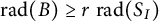
$\tau \left ( C^1,\{S_I^1\}_I\right )\tau \left ( C^2,\{S_L^2\}_L\right ) \geq \frac {1}{(1-2r)^2},$
-
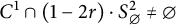
(2)
$C^1\cap (1-2r)\cdot S_\emptyset ^2\neq \emptyset $
, -
(3)
$\operatorname {\mathrm {rad}}(S_\emptyset ^1)\geq r\, \operatorname {\mathrm {rad}}(S_\emptyset ^2)$
, -
(4)
$\{S_I^1\}_I$
and
$\{S_L^2\}_L$
are r-uniformly dense.


Then,
 $C^1\cap C^2 \neq \emptyset $
.
$C^1\cap C^2 \neq \emptyset $
.
Remark 3.3 While there are other higher-dimensional notions of thickness, see, for instance, [Reference Biebler3, Reference Falconer and Yavicoli11], we choose to use Yavicoli’s higher-dimensional notion of thickness as it is simpler to construct subsets A, B of C with thickness comparable to C.
3.1 Computing the thickness of a subset
We now consider how to compute the thickness of a subset of C given the thickness of C.
Let C be a compact set with a system of balls
 $\{S_I\}_I$
, and let
$\{S_I\}_I$
, and let
 $A:= S_{1_A}\cap C$
for some
$A:= S_{1_A}\cap C$
for some
 $1\leq 1_A\leq k_\emptyset $
be a compact set with a system of balls
$1\leq 1_A\leq k_\emptyset $
be a compact set with a system of balls
 $\{S_{1_A,I}\}_I$
.
$\{S_{1_A,I}\}_I$
.
While the definition of
 $h_I(C):=\max _{x\in S_I} \operatorname {\mathrm {dist}}(x,C)$
is used in calculating the thickness of C, when we consider the thickness of first generation subsets of the form
$h_I(C):=\max _{x\in S_I} \operatorname {\mathrm {dist}}(x,C)$
is used in calculating the thickness of C, when we consider the thickness of first generation subsets of the form
 $A=C \cap S_{1_A}$
for some
$A=C \cap S_{1_A}$
for some
 $1_A$
satisfying
$1_A$
satisfying
 $1\leq 1_A\leq k_\emptyset $
, we need
$1\leq 1_A\leq k_\emptyset $
, we need
 $h_{1_A}(A):=\max _{x\in S_{1_A,I}}\operatorname {\mathrm {dist}}(x,A)$
to calculate the thickness of A:
$h_{1_A}(A):=\max _{x\in S_{1_A,I}}\operatorname {\mathrm {dist}}(x,A)$
to calculate the thickness of A:
 $$ \begin{align*} \tau\left( A,\{S_{1_A,I}\}_I\right):=\inf_{n\in\mathbb{N}_0}\inf_{\ell(I)=n}\frac{\min_i \operatorname{\mathrm{rad}}(S_{1_A,I,i})}{\max_{x\in S_{1_A,I}}\operatorname{\mathrm{dist}}(x,A)}. \end{align*} $$
In the proof of Theorem 2.8, we have implicit assumptions about
 $\max _{x\in S_I}\operatorname {\mathrm {dist}}(x,C)$
but no assumptions about
$\max _{x\in S_I}\operatorname {\mathrm {dist}}(x,C)$
but no assumptions about
 $\max _{x\in S_{1_A,I}}\operatorname {\mathrm {dist}}(x,A)$
, so we use
$\max _{x\in S_{1_A,I}}\operatorname {\mathrm {dist}}(x,A)$
, so we use
 $\max _{x\in S_{1_A}}\operatorname {\mathrm {dist}}(x,C)$
to get an upper bound on
$\max _{x\in S_{1_A}}\operatorname {\mathrm {dist}}(x,C)$
to get an upper bound on
 $\max _{x\in S_{1_A}}\operatorname {\mathrm {dist}}(x,A)$
in Lemma 3.4. As in (3.2), define
$\max _{x\in S_{1_A}}\operatorname {\mathrm {dist}}(x,A)$
in Lemma 3.4. As in (3.2), define
 $$ \begin{align} h_\emptyset(C) := \max_{x\in S_\emptyset} \operatorname{\mathrm{dist}}(x,C) \quad \text{and} \quad h_{1_A}(A) &:= \max_{x\in S_{1_A}} \operatorname{\mathrm{dist}}(x,A) \nonumber\\ &= \max_{x\in S_{1_A}} \operatorname{\mathrm{dist}}(x,S_{1_A}\cap C). \end{align} $$
Lemma 3.4 (Preliminary computation for the thickness of a subset)
Let C be a compact set in (
 $\mathbb {R}^d,\operatorname {\mathrm {dist}}$
) generated by the system of balls
$\mathbb {R}^d,\operatorname {\mathrm {dist}}$
) generated by the system of balls
 $\{S_I\}_I$
such that
$\{S_I\}_I$
such that
 $\tau \left ( C,\{S_I\}\right )\geq 1$
. Then, for any word I, we have
$\tau \left ( C,\{S_I\}\right )\geq 1$
. Then, for any word I, we have
 $$ \begin{align*} \max_{x\in S_I} \operatorname{\mathrm{dist}}(x,S_I\cap C) \,\, \leq \,\, 2\max_{x\in S_I} \operatorname{\mathrm{dist}}(x,C). \end{align*} $$
So, if
 $A = S_{1_A}\cap C$
for some
$A = S_{1_A}\cap C$
for some
 $1\le 1_A \le k_\emptyset $
, Lemma 3.4 implies that
$1\le 1_A \le k_\emptyset $
, Lemma 3.4 implies that
 $$ \begin{align*} \max_{x\in S_{1_A}} \operatorname{\mathrm{dist}}(x,S_{1_A}\cap C) \,\, \leq \,\, 2\max_{x\in S_{1_A}} \operatorname{\mathrm{dist}}(x,C) \,\, \leq \,\, 2\max_{x\in S_\emptyset} \operatorname{\mathrm{dist}}(x,C), \end{align*} $$
and it follows that
 $$ \begin{align*} h_{1_A}(A) \le 2h_\emptyset(C). \end{align*} $$
Proof Fix a word I. Since
 $\tau \left ( C,\{S_I\}\right )\geq 1$
for all words I, it follows from the definition of thickness that
$\tau \left ( C,\{S_I\}\right )\geq 1$
for all words I, it follows from the definition of thickness that
 $$ \begin{align*}\min_i \operatorname{\mathrm{rad}}(S_{I,i})\geq \max_{x\in S_I}\operatorname{\mathrm{dist}}(x,C) = h_I.\end{align*} $$
In particular,
 $$ \begin{align*}\operatorname{\mathrm{rad}}(S_I)\geq \min_i \operatorname{\mathrm{rad}}(S_{I,i}) \geq h_I.\end{align*} $$
This establishes that, for any
 $y\in S_I$
, there exists a ball of radius
$y\in S_I$
, there exists a ball of radius
 $h_I$
in
$h_I$
in
 $S_I$
containing y.
$S_I$
containing y.
Now take any
 $y\in S_I$
, and observe that
$y\in S_I$
, and observe that
 $$ \begin{align*}\operatorname{\mathrm{dist}}(y,C\cap S_I)\leq \operatorname{\mathrm{dist}}(y,c'),\end{align*} $$
for any
 $c'\in C\cap S_I$
. We will choose
$c'\in C\cap S_I$
. We will choose
 $c'$
in such a way that we can bound
$c'$
in such a way that we can bound
 $\max _{x\in S_I}\operatorname {\mathrm {dist}}(x,C\cap S_I)$
.
$\max _{x\in S_I}\operatorname {\mathrm {dist}}(x,C\cap S_I)$
.
Let
 $\bar {B}_y$
be a closed ball of radius
$\bar {B}_y$
be a closed ball of radius
 $h_I$
in
$h_I$
in
 $S_I$
containing the point y. Then, there exists some point
$S_I$
containing the point y. Then, there exists some point
 $z \in \bar {B}_y\subset S_I$
such that
$z \in \bar {B}_y\subset S_I$
such that
 $$ \begin{align} \operatorname{\mathrm{dist}}(y,z)\leq h_I \quad \text{and}\quad \operatorname{\mathrm{dist}}(z,\partial S_I)\geq h_I. \end{align} $$
For instance, z can be taken as the center of
 $\bar {B}_y$
. As a consequence of the latter inequality above combined with the definition of
$\bar {B}_y$
. As a consequence of the latter inequality above combined with the definition of
 $h_I: = \max _{x\in S_I}\operatorname {\mathrm {dist}}(x,C)$
, there exists some
$h_I: = \max _{x\in S_I}\operatorname {\mathrm {dist}}(x,C)$
, there exists some
 $c'\in C \cap S_I$
such that
$c'\in C \cap S_I$
such that
 $$ \begin{align} \operatorname{\mathrm{dist}}(z,c')\leq h_I. \end{align} $$
Now, we have
 $$ \begin{align} \operatorname{\mathrm{dist}}(y,C\cap S_I) \leq \operatorname{\mathrm{dist}}(y,c') \leq \operatorname{\mathrm{dist}}(y,z) + \operatorname{\mathrm{dist}}(z,c') \leq 2h_I. \end{align} $$
As this holds for any
 $y\in S_I$
, we have
$y\in S_I$
, we have
 $$ \begin{align*} \max_{y\in S_I}\operatorname{\mathrm{dist}}(y,C \cap S_I) \leq 2 h_I. \end{align*} $$
Now that we understand the relationship in Lemma 3.4, we can use it to calculate the relationship between the thicknesses of C and its subsets.
Lemma 3.5 (Thickness of a subset)
Let C be a compact set in
 $(\mathbb {R}^d,\operatorname {\mathrm {dist}})$
generated by the system of balls
$(\mathbb {R}^d,\operatorname {\mathrm {dist}})$
generated by the system of balls
 $\{S_I\}_I$
such that
$\{S_I\}_I$
such that
 $\tau \left ( C,\{S_I\}\right )\geq 1$
. Suppose that there exists some
$\tau \left ( C,\{S_I\}\right )\geq 1$
. Suppose that there exists some
 $1\leq 1_A\leq k_\emptyset $
such that
$1\leq 1_A\leq k_\emptyset $
such that
 $S_{1_A}\cap S_i =\emptyset $
for all
$S_{1_A}\cap S_i =\emptyset $
for all
 $i\neq 1_A$
,
$i\neq 1_A$
,
 $1\le i\le k_\emptyset $
. Let
$1\le i\le k_\emptyset $
. Let
 $A= S_{1_A}\cap C$
. Then
$A= S_{1_A}\cap C$
. Then
 $$ \begin{align*}\tau\left( A,\{S_{1_A,I}\}\right) \geq \frac{1}{2}\tau\left( C,\{S_I\}\right).\end{align*} $$
Remark 3.6 We comment on the assumption that
 $S_{1_A}$
and
$S_{1_A}$
and
 $S_{1_B}$
are disjoint from all other first-generation children. Let C be a compact set generated by
$S_{1_B}$
are disjoint from all other first-generation children. Let C be a compact set generated by
 $\{S_I\}_I$
and take any
$\{S_I\}_I$
and take any
 $S_{1_A}$
a first-generation child, not necessarily disjoint from other first-generation children. Consider the following two subsets constructed by the first-generation child
$S_{1_A}$
a first-generation child, not necessarily disjoint from other first-generation children. Consider the following two subsets constructed by the first-generation child
 $S_{1_A}$
of C:
$S_{1_A}$
of C:
 $A'$
generated by the system of balls
$A'$
generated by the system of balls
 $\{S_{1_A,I}\}_{1_A,I}$
and
$\{S_{1_A,I}\}_{1_A,I}$
and
 $A := S_{1_A}\cap C$
. We necessarily have
$A := S_{1_A}\cap C$
. We necessarily have
 $A'\subseteq A \subseteq C$
.
$A'\subseteq A \subseteq C$
.
To calculate the Yavicoli thickness of a compact set E, we need:
 $(1)$
a system of balls that generates E and
$(1)$
a system of balls that generates E and
 $(2)$
the value of
$(2)$
the value of
 $\max _{x\in S_{I}}\operatorname {\mathrm {dist}}(x,E)$
for all words I. In particular, we want to calculate the thickness of a subset of a compact set, so we additionally need
$\max _{x\in S_{I}}\operatorname {\mathrm {dist}}(x,E)$
for all words I. In particular, we want to calculate the thickness of a subset of a compact set, so we additionally need
 $(1')$
a system of balls that generates the subset and relates to the system that generates C and
$(1')$
a system of balls that generates the subset and relates to the system that generates C and
 $(2')$
the value of
$(2')$
the value of
 $\max _{x\in S_{I}}\operatorname {\mathrm {dist}}(x,E)$
compared to
$\max _{x\in S_{I}}\operatorname {\mathrm {dist}}(x,E)$
compared to
 $\max _{x\in S_I} \operatorname {\mathrm {dist}}(x,C)$
. For A, we have
$\max _{x\in S_I} \operatorname {\mathrm {dist}}(x,C)$
. For A, we have
 $(2')$
as we can use Lemma 3.4 to obtain the estimate
$(2')$
as we can use Lemma 3.4 to obtain the estimate
 $$ \begin{align*}\max_{x\in S_{1_A}}\operatorname{\mathrm{dist}}(x,A) \leq 2 \max_{x\in S_{1_A}}\operatorname{\mathrm{dist}}(x,C).\end{align*} $$
While the compact set
 $A'$
generated by
$A'$
generated by
 $\{S_{1_A,I}\}$
is contained in A, if
$\{S_{1_A,I}\}$
is contained in A, if
 $S_{1_A}$
is not disjoint from other first-generation children it is possible we have some point
$S_{1_A}$
is not disjoint from other first-generation children it is possible we have some point
 $x\in S_i\cap S_{1_A}$
that is not generated by
$x\in S_i\cap S_{1_A}$
that is not generated by
 $\{S_{1_A,I}\}$
, and it becomes hard to see if A satisfies
$\{S_{1_A,I}\}$
, and it becomes hard to see if A satisfies
 $(1')$
. For
$(1')$
. For
 $A'$
, we have
$A'$
, we have
 $(1')$
because
$(1')$
because
 $A'$
is generated by
$A'$
is generated by
 $\{S_{1_A,I}\}$
, but it does not necessarily satisfy
$\{S_{1_A,I}\}$
, but it does not necessarily satisfy
 $(2')$
as we have no way to calculate or bound
$(2')$
as we have no way to calculate or bound
 $\max _{x\in S_{I}}\operatorname {\mathrm {dist}}(x,A')$
above; in general,
$\max _{x\in S_{I}}\operatorname {\mathrm {dist}}(x,A')$
above; in general,
 $$ \begin{align*}\max_{x\in S_I}\operatorname{\mathrm{dist}}(x,A')\geq \max_{x\in S_I}\operatorname{\mathrm{dist}}(x,A).\end{align*} $$
In order to guarantee the existence of a set that satisfies both
 $(1')$
and
$(1')$
and
 $(2')$
, we take
$(2')$
, we take
 $S_{1_A}$
to be disjoint from all other first-generation children. This forces
$S_{1_A}$
to be disjoint from all other first-generation children. This forces
 $A=A'$
, so
$A=A'$
, so
 $(1')$
and
$(1')$
and
 $(2')$
are both satisfied. We first need a corresponding system of balls that generate the set. In the case of
$(2')$
are both satisfied. We first need a corresponding system of balls that generate the set. In the case of
 $A=S_{1_A}\cap C$
, the system of balls
$A=S_{1_A}\cap C$
, the system of balls
 $\{S_{1_A,I}\}$
generates the set
$\{S_{1_A,I}\}$
generates the set
 $A=S_{1_A}\cap C$
if and only if all elements of
$A=S_{1_A}\cap C$
if and only if all elements of
 $S_{1_A}\cap C$
are generated by
$S_{1_A}\cap C$
are generated by
 $\{S_{1_A,I}\}$
. This is satisfied by having
$\{S_{1_A,I}\}$
. This is satisfied by having
 $S_{1_A}$
disjoint from all other first-generation children
$S_{1_A}$
disjoint from all other first-generation children
 $S_i$
where
$S_i$
where
 $1\leq i\leq k_\emptyset $
,
$1\leq i\leq k_\emptyset $
,
 $i\neq 1_A$
.
$i\neq 1_A$
.
Proof Lemma 3.4 implies
 $$ \begin{align*} \max_{x\in S_{I}}\operatorname{\mathrm{dist}}(x,A) := \max_{x\in S_{I}}\operatorname{\mathrm{dist}} (x,S_{1_A}\cap C) \leq 2\max_{x\in S_{I}}\operatorname{\mathrm{dist}}(x,C), \end{align*} $$
for all words I starting at
 $1_A$
. It follows that:
$1_A$
. It follows that:
 $$ \begin{align*} \tau\left( A, \{S_{1_A,I}\}\right) &= \inf_{n\geq 1} \inf_{\substack{\ell(I)=n\\ I=\{1_A,\ldots\}}} \frac{\min_i \operatorname{\mathrm{rad}}(S_{I,i})}{\max_{x\in S_{I}} \operatorname{\mathrm{dist}}(x,A)} \geq \frac{1}{2}\inf_{n\geq1} \inf_{\substack{\ell(I)=n\\I=\{1_A,\ldots\} }} \frac{\min_i \operatorname{\mathrm{rad}}(S_{I,i})}{\max_{x\in S_{I}} \operatorname{\mathrm{dist}}(x,C)} \\ &\geq \frac{1}{2}\inf_{n\geq0} \inf_{\ell(I)=n} \frac{\min_i \operatorname{\mathrm{rad}}(S_{I,i})}{\max_{x\in S_I} \operatorname{\mathrm{dist}}(x,C)} =\frac{1}{2}\tau\left( C, \{S_I\}\right), \end{align*} $$
where the first inequality follows from the estimate in Lemma 3.4, and the second inequality follows from taking the infimum over a larger set.
The content of these lemmas is significantly different from the one-dimensional case and reflect one of the technical hurdles of defining thickness in higher dimensions. In the one-dimensional setting, if
 $C\subset \mathbb {R}$
and
$C\subset \mathbb {R}$
and
 $\tau $
denotes Newhouse thickness, then
$\tau $
denotes Newhouse thickness, then
 $\tau (A)\geq \tau (C)$
whenever
$\tau (A)\geq \tau (C)$
whenever
 $A=C\cap S$
and S is bridge. In the Appendix, we illustrate this key difference and discuss a special case in which Lemma 3.5, and hence our main results, can be improved.
$A=C\cap S$
and S is bridge. In the Appendix, we illustrate this key difference and discuss a special case in which Lemma 3.5, and hence our main results, can be improved.
4 Proof of main results that use Newhouse thickness
This section contains the proofs of Proposition 2.1 and Theorem 2.2.
4.1 Proof of Proposition 2.1
The following proof is inspired by that of Yavicoli’s [Reference Yavicoli39, Proposition 20], where the proposition is proved for
 $\lambda =\frac{1}{2}$
. The proof here is more involved as a number of technical hurdles arise in this more general setting.
$\lambda =\frac{1}{2}$
. The proof here is more involved as a number of technical hurdles arise in this more general setting.
Since thickness is invariant under scaling and translations, we may assume that
 $\operatorname {\mathrm {conv}}(C)=[0,1]$
. The idea is to show that
$\operatorname {\mathrm {conv}}(C)=[0,1]$
. The idea is to show that
 $C\cap \left ( (1-\lambda )C + \lambda C \right ) \neq \emptyset $
for
$C\cap \left ( (1-\lambda )C + \lambda C \right ) \neq \emptyset $
for
 $\lambda \in (0,1)$
. To avoid degeneracy, we introduce disjoint subsets A and B of C, and show that
$\lambda \in (0,1)$
. To avoid degeneracy, we introduce disjoint subsets A and B of C, and show that
 $C\cap \left ( (1-\lambda )A + \lambda B \right ) \neq \emptyset $
, which will establish that there exist points
$C\cap \left ( (1-\lambda )A + \lambda B \right ) \neq \emptyset $
, which will establish that there exist points
 $a,b \in C$
with
$a,b \in C$
with
 $a\neq b$
so that
$a\neq b$
so that
 $$ \begin{align*}\{a, (1-\lambda)a + \lambda b, b\} \subset C.\end{align*} $$
A brief sketch of the proof is as follows. We observe that
 $t\in (1-\lambda )A+ \lambda B$
if and only if
$t\in (1-\lambda )A+ \lambda B$
if and only if
 $ -(1-\lambda )A \cap \left (\lambda B-t\right ) \neq \emptyset. $
We then verify the hypotheses of the Gap Lemma and apply it to the sets
$ -(1-\lambda )A \cap \left (\lambda B-t\right ) \neq \emptyset. $
We then verify the hypotheses of the Gap Lemma and apply it to the sets
 $-(1-\lambda )A$
and
$-(1-\lambda )A$
and
 $ \left (\lambda B-t\right )$
. A potential issue that can arise is that, for
$ \left (\lambda B-t\right )$
. A potential issue that can arise is that, for
 $\lambda $
small,
$\lambda $
small,
 $ \left (\lambda B-t\right )$
can be contained in a gap of
$ \left (\lambda B-t\right )$
can be contained in a gap of
 $-(1-\lambda )A$
, which would violate the hypotheses of the gap lemma. To get around this obstacle, we only work with values of t and
$-(1-\lambda )A$
, which would violate the hypotheses of the gap lemma. To get around this obstacle, we only work with values of t and
 $\lambda $
that avoid this issue, mainly so that the two sets are interwoven and neither lies in the gap of the other.
$\lambda $
that avoid this issue, mainly so that the two sets are interwoven and neither lies in the gap of the other.
Let
 $G=(k_1, k_2)$
denote the largest bounded gap of C. Set
$G=(k_1, k_2)$
denote the largest bounded gap of C. Set
 $A=C\cap [0,k_1]$
and
$A=C\cap [0,k_1]$
and
 $B=C\cap [k_2, 1]$
, and denote
$B=C\cap [k_2, 1]$
, and denote
 $|A| = k_1$
and
$|A| = k_1$
and
 $|B| = 1-k_2$
.
$|B| = 1-k_2$
.
Set
 $$ \begin{align*}m = |A|/(|A|+|B|),\end{align*} $$
 $$ \begin{align*}I_\lambda = [\lambda k_2, \lambda + (1-\lambda)k_1]\end{align*} $$
and
 $$ \begin{align*}\widetilde{I}_\lambda = [\lambda k_2, \lambda] \,\, \bigcup \,\, [\lambda k_2 +(1-\lambda) k_1, \lambda + (1-\lambda)k_1].\end{align*} $$
First, we use the gap lemma to establish the following claim.
Claim 4.1 For
 $\lambda \in (0,1)$
,
$\lambda \in (0,1)$
,
 $$ \begin{align*}\widetilde{I}_\lambda \,\, \subset \,\, (1-\lambda)A+ \lambda B \,\,\subset\,\, I_\lambda.\end{align*} $$
Proof We verify the first containment; the second containment is straightforward.
Let
 $t \in \widetilde {I}_\lambda $
, and observe
$t \in \widetilde {I}_\lambda $
, and observe
 $t\in (1-\lambda )A+ \lambda B$
if and only if
$t\in (1-\lambda )A+ \lambda B$
if and only if
 $$ \begin{align} -(1-\lambda)A \cap \left(\lambda B-t\right) \neq \emptyset. \end{align} $$
We verify the hypotheses of the gap lemma and apply it to the sets
 $-(1-\lambda )A $
and
$-(1-\lambda )A $
and
 $ \left (\lambda B-t\right )$
to verify (4.1) for
$ \left (\lambda B-t\right )$
to verify (4.1) for
 $t\in \widetilde {I}_\lambda $
.
$t\in \widetilde {I}_\lambda $
.
First, we verify that the convex hulls,
 $\operatorname {\mathrm {conv}}(-(1-\lambda )A)$
and
$\operatorname {\mathrm {conv}}(-(1-\lambda )A)$
and
 $\operatorname {\mathrm {conv}}(\lambda B-t)$
, are interwoven for
$\operatorname {\mathrm {conv}}(\lambda B-t)$
, are interwoven for
 $t\in \widetilde {I}_\lambda $
, where we say that two closed intervals are interwoven if they intersect and neither is contained in the interior of the other.
$t\in \widetilde {I}_\lambda $
, where we say that two closed intervals are interwoven if they intersect and neither is contained in the interior of the other.
Observe
 $$ \begin{align*}\operatorname{\mathrm{conv}}(-(1-\lambda)A) = [ - (1-\lambda) k_1, 0],\end{align*} $$
and
 $$ \begin{align*}\operatorname{\mathrm{conv}}(\lambda B-t) = [\lambda k_2 -t, \lambda -t].\end{align*} $$
It follows that the convex hulls are interwoven provided that either
 $$ \begin{align} \lambda k_2 -t \le -(1-\lambda)k_1 \le \lambda -t \le 0 \end{align} $$
or
 $$ \begin{align} -(1-\lambda)k_1 \le \lambda k_2 -t \le 0 \le \lambda -t. \end{align} $$
These simplify to the conditions that, from (4.2),
 $$ \begin{align*}t\in [\lambda k_2 + (1-\lambda) k_1,\,\, \lambda + (1-\lambda) k_1],\end{align*} $$
or, from (4.3), the condition that
 $$ \begin{align*}t\in [\lambda k_2, \,\, \min\{ \lambda, \lambda k_2 + (1-\lambda) k_1\},\end{align*} $$
where we observe that
 $\min \{ \lambda , \lambda k_2+ (1-\lambda ) k_1,\} = \lambda \iff \lambda \le m.$
Taking the union, we see that the convex hulls are interwoven provided that
 $$ \begin{align*}t\in \widetilde{I}_\lambda.\end{align*} $$
The interwoven condition guarantees that sets
 $-(1-\lambda )A$
and
$-(1-\lambda )A$
and
 $(\lambda B-t)$
are not contained in each others’ gaps.
$(\lambda B-t)$
are not contained in each others’ gaps.
Finally, we observe that
 $\tau (A) = \tau ( C\cap [0, k_1]) \geq \tau (C)$
. In general, thickness may behave badly under intersections, but
$\tau (A) = \tau ( C\cap [0, k_1]) \geq \tau (C)$
. In general, thickness may behave badly under intersections, but
 $\tau (C\cap [0, k_1]) \geq \tau (C)$
since G is the largest gap of C. Similarly,
$\tau (C\cap [0, k_1]) \geq \tau (C)$
since G is the largest gap of C. Similarly,
 $\tau (B)\geq \tau (C)$
. It follows that
$\tau (B)\geq \tau (C)$
. It follows that
 $$ \begin{align*}\tau(-(1-\lambda)A) \tau( \lambda B-t) \geq 1,\end{align*} $$
and the gap lemma applies.
The next step is to show that
 $\widetilde {I}_\lambda \cap C \neq \emptyset ,$
which will suffice to establish that
$\widetilde {I}_\lambda \cap C \neq \emptyset ,$
which will suffice to establish that
 $((1-\lambda )A + \lambda B) \cap C \neq \emptyset $
by the previous claim. Recall
$((1-\lambda )A + \lambda B) \cap C \neq \emptyset $
by the previous claim. Recall
 $$ \begin{align*}\widetilde{I}_\lambda = [\lambda k_2, \lambda] \,\, \bigcup \,\, [\lambda k_2 +(1-\lambda) k_1, \lambda + (1-\lambda)k_1].\end{align*} $$
Claim 4.2 If
 $\lambda \in (0,1)$
, then
$\lambda \in (0,1)$
, then
 $C\cap \left ( (1-\lambda ) A + \lambda B\right ) \neq \emptyset $
.
$C\cap \left ( (1-\lambda ) A + \lambda B\right ) \neq \emptyset $
.
Proof We prove the claim for
 $\lambda \geq \frac{1}{2}$
. Then, by applying the result to
$\lambda \geq \frac{1}{2}$
. Then, by applying the result to
 $\widetilde {C} = -C+1$
, we may conclude the claim holds for any
$\widetilde {C} = -C+1$
, we may conclude the claim holds for any
 $\lambda \in (0,1)$
. Recall
$\lambda \in (0,1)$
. Recall
 $G=(k_1, k_2)$
denotes the largest bounded gap of C.
$G=(k_1, k_2)$
denotes the largest bounded gap of C.
Let
 $\lambda \geq \frac{1}{2}$
. We consider the cases when
$\lambda \geq \frac{1}{2}$
. We consider the cases when
 $|A| \le |B|$
and
$|A| \le |B|$
and
 $|B| \le |A|$
separately.
$|B| \le |A|$
separately.
Case 1: Suppose first that
 $|A| \le |B|$
so that
$|A| \le |B|$
so that
 $k_1 \le 1-k_2$
or
$k_1 \le 1-k_2$
or
 $$ \begin{align} k_2 \le 1-k_1. \end{align} $$
Since
 $\tau (C)\geq 1$
, it follows that
$\tau (C)\geq 1$
, it follows that
 $|A| \geq |G|$
so that
$|A| \geq |G|$
so that
 $k_1\geq k_2-k_1$
or that
$k_1\geq k_2-k_1$
or that
 $$ \begin{align} k_2 \le 2k_1. \end{align} $$
Observe
 $k_2 \in \widetilde {I}_\lambda $
. Indeed,
$k_2 \in \widetilde {I}_\lambda $
. Indeed,
 $$ \begin{align} \lambda k_2 +(1-\lambda)k_1 \le k_2 \le \lambda + (1-\lambda)k_1, \end{align} $$
where the first inequality holds trivially since such a convex combination of
 $k_1< k_2$
is bounded above by
$k_1< k_2$
is bounded above by
 $k_2$
, and for the second inequality is implied, see by graphing, by (4.4) and (4.5) provided
$k_2$
, and for the second inequality is implied, see by graphing, by (4.4) and (4.5) provided
 $\lambda \in [\frac 12, 1)$
.
$\lambda \in [\frac 12, 1)$
.
Case 2: Suppose second that
 $|B| \le |A|$
so that
$|B| \le |A|$
so that
 $ 1-k_2 \le k_1$
or
$ 1-k_2 \le k_1$
or
 $$ \begin{align} 1-k_1 \le k_2. \end{align} $$
Since
 $\tau (C)\geq 1$
, it follows that
$\tau (C)\geq 1$
, it follows that
 $|B| \geq |G|$
so that
$|B| \geq |G|$
so that
 $1-k_2\geq k_2-k_1$
or that
$1-k_2\geq k_2-k_1$
or that
 $$ \begin{align} k_2 \le \frac12(1+k_1). \end{align} $$
Again, observe that
 $k_2 \in \widetilde {I}_\lambda $
. Indeed, as above, we must verify
$k_2 \in \widetilde {I}_\lambda $
. Indeed, as above, we must verify
 $$ \begin{align} \lambda k_2 +(1-\lambda)k_1 \le k_2 \le \lambda + (1-\lambda)k_1, \end{align} $$
where the first inequality is implied in the same way as above, and the second is implied by noting that, by (4.8),
 $k_2 \le \frac 12(1+k_1),$
and
$k_2 \le \frac 12(1+k_1),$
and
 $\frac 12(1+k_1) \le \lambda + (1-\lambda )k_1 $
provided
$\frac 12(1+k_1) \le \lambda + (1-\lambda )k_1 $
provided
 $\lambda \in [\frac 12, 1]$
.
$\lambda \in [\frac 12, 1]$
.
4.2 Proof of Theorem 2.2
Let T be a set of three distinct vertices in
 $\mathbb {R}^2$
. We prove that if
$\mathbb {R}^2$
. We prove that if
 $C\subset \mathbb {R}$
is compact with
$C\subset \mathbb {R}$
is compact with
 $\tau (C)\geq 1$
, then
$\tau (C)\geq 1$
, then
 $C\times C$
contains a similar copy of T.
$C\times C$
contains a similar copy of T.
If all three vertices lie on a line, the result follows from Proposition 2.1, after rotating the line to be parallel to one of the axes, if necessary. We assume then that the vertices are not collinear.
Label the vertices of
 $T\subset \mathbb {R}^2$
by
$T\subset \mathbb {R}^2$
by
 $x=(x_1,x_2)$
,
$x=(x_1,x_2)$
,
 $y=(y_1,y_2)$
, and
$y=(y_1,y_2)$
, and
 $z=(z_1,z_2)$
, with corresponding angles
$z=(z_1,z_2)$
, with corresponding angles
 $\theta _1, \theta _2, \theta _3$
, with
$\theta _1, \theta _2, \theta _3$
, with
 $\theta _3 \geq \theta _i$
for
$\theta _3 \geq \theta _i$
for
 $i=1,2$
. Further, performing a rotation and reflection, assume that T is positioned and labeled so that x and y lie on the x-axis, and
$i=1,2$
. Further, performing a rotation and reflection, assume that T is positioned and labeled so that x and y lie on the x-axis, and
 $z_2>0$
. It follows that
$z_2>0$
. It follows that
 $x_1\le z_1\le y_1$
.
$x_1\le z_1\le y_1$
.
Label
 $h = z_2$
,
$h = z_2$
,
 $b_1= (z_1-x_1)$
,
$b_1= (z_1-x_1)$
,
 $b_2= (y_1-z_1)$
, and
$b_2= (y_1-z_1)$
, and
 $b= b_1+b_2$
. It follows that
$b= b_1+b_2$
. It follows that
 $$ \begin{align} h= \tan{\theta_1}b_1 = \tan{\theta_2}b_2. \end{align} $$
Since
 $\tau (C)\geq 1$
, it is a consequence of the Newhouse gap lemma that
$\tau (C)\geq 1$
, it is a consequence of the Newhouse gap lemma that
 $\Delta (C)$
has non-empty interior. Further, there exists
$\Delta (C)$
has non-empty interior. Further, there exists
 $L>0$
so that
$L>0$
so that
 $[0,L]\subset \Delta (C)$
.
$[0,L]\subset \Delta (C)$
.
Choose
 $c>0$
so that
$c>0$
so that
 $ch\le L$
and
$ch\le L$
and
 $cb\le L$
. Choose
$cb\le L$
. Choose
 $c'\in (0,c]$
and
$c'\in (0,c]$
and
 $t\in \mathbb {R}$
so that
$t\in \mathbb {R}$
so that
 $P = \{c'x_1+t, c'z_1+t, c'y_1+t\}\subset C$
; such a choice is possible by Proposition 2.1. Choose
$P = \{c'x_1+t, c'z_1+t, c'y_1+t\}\subset C$
; such a choice is possible by Proposition 2.1. Choose
 $a,b\in C$
so that
$a,b\in C$
so that
 $b-a = c'h$
.
$b-a = c'h$
.
Now, the triangle with vertices
 $$ \begin{align} (c'x_1+t, a), (c'y_1+t, a), (c'z_1+t, b) \end{align} $$
is similar to T and each of the points in (4.11) are in C.
5 Proof of main results that use Yavicoli thickness
We use the notation and definitions from Section 3 throughout this section. Each
 $S_I$
is a closed ball with center,
$S_I$
is a closed ball with center,
 $c_I$
, and radius,
$c_I$
, and radius,
 $t_I$
, which is denoted by
$t_I$
, which is denoted by
 $\bar {B}(c_I,t_I)$
. Each
$\bar {B}(c_I,t_I)$
. Each
 $S_I$
has a finite number of children. The number of first-generation children of C is denoted by
$S_I$
has a finite number of children. The number of first-generation children of C is denoted by
 $k_\emptyset $
, so for any
$k_\emptyset $
, so for any
 $1\leq i\leq k_\emptyset $
we have that
$1\leq i\leq k_\emptyset $
we have that
 $S_i$
is a first-generation child with radius
$S_i$
is a first-generation child with radius
 $t_i=\operatorname {\mathrm {rad}}(S_i)$
. Without loss of generality, we label the
$t_i=\operatorname {\mathrm {rad}}(S_i)$
. Without loss of generality, we label the
 $k_\emptyset $
first-generation children to be ordered by nondecreasing radius size:
$k_\emptyset $
first-generation children to be ordered by nondecreasing radius size:
 $$ \begin{align*}t_1\leq t_2\leq \cdots \leq t_{k_\emptyset}.\end{align*} $$
The set
 $\lambda A + (1-\lambda )B$
denotes the convex combination of the set
$\lambda A + (1-\lambda )B$
denotes the convex combination of the set
 $\left \{ \lambda a + (1-\lambda )b : a\in A, b\in B\right \}$
, and
$\left \{ \lambda a + (1-\lambda )b : a\in A, b\in B\right \}$
, and
 $\lambda D$
denotes the ball D with center and radius scaled by
$\lambda D$
denotes the ball D with center and radius scaled by
 $\lambda $
. We write
$\lambda $
. We write
 $t\cdot C$
to denote the ball with the same center as C and radius equal to
$t\cdot C$
to denote the ball with the same center as C and radius equal to
 $t\operatorname {\mathrm {rad}}(C)$
.
$t\operatorname {\mathrm {rad}}(C)$
.
The proofs of this section have a common setup and set of notation.
5.1 Setup and table of notation for the proofs of Theorems 2.8 and 2.12
Throughout,
 $C\subset \mathbb {R}^d$
denotes a compact set generated by the system of balls
$C\subset \mathbb {R}^d$
denotes a compact set generated by the system of balls
 $\{S_I\}_I$
in the distance
$\{S_I\}_I$
in the distance
 $\operatorname {\mathrm {dist}}$
generated by the norm
$\operatorname {\mathrm {dist}}$
generated by the norm
 $\|\cdot \|$
as expected:
$\|\cdot \|$
as expected:
 $\operatorname {\mathrm {dist}}(x,C) = \min _{y\in C}\|x-y\|$
. Because thickness is translation and scalar invariant, we assume that
$\operatorname {\mathrm {dist}}(x,C) = \min _{y\in C}\|x-y\|$
. Because thickness is translation and scalar invariant, we assume that
 $C\subset \bar {B}(0,1)$
, so that
$C\subset \bar {B}(0,1)$
, so that
 $S_\emptyset = \bar {B}(0,1)$
, where
$S_\emptyset = \bar {B}(0,1)$
, where
 $\bar {B}(x,t)= \{x \in \mathbb {R}^d: \|x\| \le t\}$
.
$\bar {B}(x,t)= \{x \in \mathbb {R}^d: \|x\| \le t\}$
.
Further,
 $S_{1_A} =\bar {B}(c_{1_A}, t_{1_A})$
and
$S_{1_A} =\bar {B}(c_{1_A}, t_{1_A})$
and
 $S_{1_B} =\bar {B}(c_{1_B}, t_{1_B})$
denote first-generation children and closed balls with centers
$S_{1_B} =\bar {B}(c_{1_B}, t_{1_B})$
denote first-generation children and closed balls with centers
 $c_{1_A}, c_{1_B}$
and radii
$c_{1_A}, c_{1_B}$
and radii
 $t_{1_A}, t_{1_B}$
, respectively, to be chosen in each proof, where the radius of
$t_{1_A}, t_{1_B}$
, respectively, to be chosen in each proof, where the radius of
 $S_{1_A}$
is assumed to be no more than the radius of
$S_{1_A}$
is assumed to be no more than the radius of
 $S_{1_B}$
:
$S_{1_B}$
:
 $$ \begin{align*}t_{1_A} \le t_{1_B}.\end{align*} $$
In the proof of Theorem 2.12, we further assume that
 $\operatorname {\mathrm {dist}}$
is Euclidean norm
$\operatorname {\mathrm {dist}}$
is Euclidean norm
 $\|\cdot \|_2$
in order to guarantee that a rotated ball is still a ball in the same norm.
$\|\cdot \|_2$
in order to guarantee that a rotated ball is still a ball in the same norm.
For convenience, we make a table of notation that will be used throughout this section, and we record some relationships between variables.

Long description
From the top row downward, the left column displays notations and the right column provides definitions. Row 1 shows B bar open parenthesis x comma t close parenthesis defined as the closed ball with center x in R to the d power and radius t greater than or equal to zero. Row 2 gives S sub empty set equals B bar open parenthesis zero comma one close parenthesis as the closed unit ball. Row 3 lists S sub 1 sub A equals B bar open parenthesis c sub 1 sub A comma t sub 1 sub A close parenthesis and S sub 1 sub B equals B bar open parenthesis c sub 1 sub B comma t sub 1 sub B close parenthesis as first generation children disjoint from all other first generation children. Row 4 defines A as S sub 1 sub A intersect C and B as S sub 1 sub B intersect C, which are disjoint subsets of C. Row 5 lists r as the fixed uniformity constant in open parenthesis zero comma one half close parenthesis. Row 6 gives h sub empty set open parenthesis C close parenthesis equals max over x in S sub empty set of dist open parenthesis x comma C close parenthesis, the maximum distance from S sub empty set to C. Row 7 defines h sub 1 sub A as h sub 1 sub A open parenthesis A close parenthesis equals max over x in S sub 1 sub A of dist open parenthesis x comma S sub 1 sub A intersect C close parenthesis, the maximum distance from S sub 1 sub A to A equals S sub 1 sub A intersect C. Row 8 gives h sub 1 sub B as h sub 1 sub B open parenthesis B close parenthesis equals max over x in S sub 1 sub B of dist open parenthesis x comma S sub 1 sub B intersect C close parenthesis, the maximum distance from S sub 1 sub B to B equals S sub 1 sub B intersect C. Row 9 lists t sub i as the radius of the first generation child S sub i.
The following is an immediate consequence of the definition of thickness, Definition 3.2, applied with
 $n=0$
and i for
$n=0$
and i for
 $1\le i\le k_\emptyset $
, and will be used throughout:
$1\le i\le k_\emptyset $
, and will be used throughout:
 $$ \begin{align} \tau\left( C,\{S_I\}\right) \leq \frac{t_{i}}{h_\emptyset}. \end{align} $$
5.2 Proof of Theorem 2.8
Fix
 $0<r<\frac {1}{2}$
and
$0<r<\frac {1}{2}$
and
 $0<\lambda \leq \frac {1}{2}$
. Let C be a compact set in
$0<\lambda \leq \frac {1}{2}$
. Let C be a compact set in
 $(\mathbb {R}^d,\operatorname {\mathrm {dist}})$
generated by the system of balls
$(\mathbb {R}^d,\operatorname {\mathrm {dist}})$
generated by the system of balls
 $\{S_I\}_I$
such that C is r-uniformly dense and
$\{S_I\}_I$
such that C is r-uniformly dense and
 $\tau \left ( C,\{S_I\}\right ) \geq \frac {2(1-\lambda )}{\lambda (1-2r)}$
. Assume
$\tau \left ( C,\{S_I\}\right ) \geq \frac {2(1-\lambda )}{\lambda (1-2r)}$
. Assume
 $C \subset S_\emptyset = \bar {B}(0,1)$
.
$C \subset S_\emptyset = \bar {B}(0,1)$
.
Our proof is motivated by the following key observation. If we were to take two disjoint subsets A, B of C and show that
 $$ \begin{align*}\left(\lambda A+ (1-\lambda) B\right) \cap C\neq\emptyset,\end{align*} $$
then there would exists some element
 $x\in \lambda A+(1-\lambda ) B$
of the form
$x\in \lambda A+(1-\lambda ) B$
of the form
 $x=\lambda a+(1-\lambda )b$
for some
$x=\lambda a+(1-\lambda )b$
for some
 $a\in A$
and
$a\in A$
and
 $b\in B$
and
$b\in B$
and
 $x \in C$
, with
$x \in C$
, with
 $a\neq b$
. Thus, C would contain the
$a\neq b$
. Thus, C would contain the
 $3$
-point convex combination
$3$
-point convex combination
 $\{a, \lambda a+(1-\lambda )b,b\}$
. We proceed with this plan in place.
$\{a, \lambda a+(1-\lambda )b,b\}$
. We proceed with this plan in place.
Set
 $A:= S_{1_A}\cap C$
and
$A:= S_{1_A}\cap C$
and
 $B:=S_{1_B}\cap C$
, where
$B:=S_{1_B}\cap C$
, where
 $1\leq 1_A<1_B\leq k_\emptyset $
, and
$1\leq 1_A<1_B\leq k_\emptyset $
, and
 $S_{1_A}$
,
$S_{1_A}$
,
 $S_{1_B}$
are disjoint first-generation children that are disjoint from all other children. Observe that our choice of A and B imply
$S_{1_B}$
are disjoint first-generation children that are disjoint from all other children. Observe that our choice of A and B imply
 $$ \begin{align} t_{1_A}\leq t_{1_B}. \end{align} $$
We express A as the compact set generated by
 $\{S_{1_A,I}\}_I$
. We express B similarly.
$\{S_{1_A,I}\}_I$
. We express B similarly.
As in (3.2), we define
 $$ \begin{align} h_\emptyset&:=h_\emptyset(C) = \max_{x\in S_\emptyset} \operatorname{\mathrm{dist}}(x,C), \quad h_{1_A}:= h_{1_A}(A) = \max_{x\in S_{1_A}} \operatorname{\mathrm{dist}}(x,A), \quad \text{and} \\ h_{1_B} &:= h_{1_B}(B)= \max_{x\in S_{1_B}}\operatorname{\mathrm{dist}}(x,B).\nonumber \end{align} $$
Recall, it is a consequence of Lemma 3.4 that
 $$ \begin{align} h_{1_A} \le 2h_\emptyset \,\,\, \text{ and } \,\,\, h_{1_B} \le 2h_\emptyset. \end{align} $$
We now prove a key lemma, which states that the set
 $\lambda A+(1-\lambda )B$
contains a disk.
$\lambda A+(1-\lambda )B$
contains a disk.
Lemma 5.1 The set
 $\lambda A+(1-\lambda )B$
contains the closed ball
$\lambda A+(1-\lambda )B$
contains the closed ball
 $$ \begin{align*} D & := \bar{B}\left(\lambda c_{1_A} + (1-\lambda) c_{1_B}, t_D\right), \end{align*} $$
where
 $t_D:= \lambda (1-2r)t_{1_A}+(1-\lambda )t_{1_B}-(1-\lambda )h_{1_B}$
.
$t_D:= \lambda (1-2r)t_{1_A}+(1-\lambda )t_{1_B}-(1-\lambda )h_{1_B}$
.
Proof of Lemma 5.1
To prove the lemma, we verify the following implications:
 $$ \begin{align} t \in D & \Rightarrow \left((1-\lambda)S_{1_B}-t\right) \cap \bar{B}\left(-\lambda c_{1_A},t_D-(1-\lambda)t_{1_B}\right)\neq \emptyset \end{align} $$
 $$ \begin{align} & \Rightarrow \left((1-\lambda)B-t\right) \cap (1-2r)\cdot \left( -\lambda S_{1_A}\right) \neq \emptyset \end{align} $$
 $$ \begin{align} & \Rightarrow \left( (1-\lambda)B-t\right)\cap\left( -\lambda A\right)\neq \emptyset. \end{align} $$
Since
 $ \left ((1-\lambda ) B-t\right )\cap (-\lambda A) \neq \emptyset $
if and only if
$ \left ((1-\lambda ) B-t\right )\cap (-\lambda A) \neq \emptyset $
if and only if
 $t\in \lambda A+(1-\lambda ) B$
, this will complete the proof of the lemma.
$t\in \lambda A+(1-\lambda ) B$
, this will complete the proof of the lemma.
The first two implications are purely geometric and follow from simple algebraic manipulations. The final implication utilizes the Gap Lemma and relies on Lemma 3.5.
Verifying implication (5.5): First, observe that the radius
 $t_D-(1-\lambda )t_{1_B}$
is in fact nonnegative. Combining our assumed lower bound on
$t_D-(1-\lambda )t_{1_B}$
is in fact nonnegative. Combining our assumed lower bound on
 $\tau \left ( C,\{S_I\}\right )$
with the upper bound in (5.1):
$\tau \left ( C,\{S_I\}\right )$
with the upper bound in (5.1):
 $$ \begin{align} \frac{2(1-\lambda)}{\lambda(1-2r)}\leq \tau\left( C,\{S_I\}\right) \leq \frac{t_{1_A}}{h_\emptyset}, \end{align} $$
which implies
 $$ \begin{align*} 2(1-\lambda)h_\emptyset \leq \lambda (1-2r) t_{1_A}. \end{align*} $$
By (5.4), we know
 $h_{1_B}\leq 2h_\emptyset $
which means
$h_{1_B}\leq 2h_\emptyset $
which means
 $$ \begin{align*} (1-\lambda)h_{1_B} \leq \lambda (1-2r) t_{1_A}, \end{align*} $$
so
 $$ \begin{align*} t_D-(1-\lambda)t_{1_B}\geq 0. \end{align*} $$
Second, let
 $t \in D$
and write
$t \in D$
and write
 $t = \lambda c_{1_A} + (1-\lambda ) c_{1_B} + x$
for some
$t = \lambda c_{1_A} + (1-\lambda ) c_{1_B} + x$
for some
 $$ \begin{align*} \|x\| \leq t_D. \end{align*} $$
Recalling
 $(1-\lambda )S_{1_B}-t = \bar {B}\left ( (1-\lambda )c_{1_B}-t,(1-\lambda )t_{1_B} \right )$
, we wish to show that
$(1-\lambda )S_{1_B}-t = \bar {B}\left ( (1-\lambda )c_{1_B}-t,(1-\lambda )t_{1_B} \right )$
, we wish to show that
 $$ \begin{align*} \bar{B}\left( (1-\lambda)c_{1_B}-t,(1-\lambda)t_{1_B} \right) \cap \bar{B}\left(-\lambda c_{1_A},t_D-(1-\lambda)t_{1_B}\right)\neq \emptyset. \end{align*} $$
By the definition of t, this holds if and only if
 $$ \begin{align*}\bar{B}\left( -\lambda c_{1_A}-x,(1-\lambda)t_{1_B} \right) \cap \bar{B}\left(-\lambda c_{1_A},t_D-(1-\lambda)t_{1_B}\right) \neq \emptyset,\end{align*} $$
which, shifting everything by
 $\lambda c_{1_A}$
, holds if and only if
$\lambda c_{1_A}$
, holds if and only if
 $$ \begin{align*}\bar{B}\left( -x,(1-\lambda)t_{1_B} \right) \cap \bar{B} \left( \vec{0}, t_D-(1-\lambda)t_{1_B} \right) \neq \emptyset,\end{align*} $$
which is true since
 $\| x\| \le t_D$
.
$\| x\| \le t_D$
.
Verifying implication (5.6): Let
 $t\in D$
. By (5.5), there exists a
$t\in D$
. By (5.5), there exists a
 $$ \begin{align*}z\in \left((1-\lambda)S_{1_B}-t\right) \cap \bar{B}\left(-\lambda c_{1_A},t_D-(1-\lambda)t_{1_B}\right).\end{align*} $$
Since
 $z \in \left ((1-\lambda )S_{1_B}-t\right )$
, we know by definition of
$z \in \left ((1-\lambda )S_{1_B}-t\right )$
, we know by definition of
 $h_{1_B}$
that there exists
$h_{1_B}$
that there exists
 $y \in (1-\lambda )B-t$
such that
$y \in (1-\lambda )B-t$
such that
 $$ \begin{align*}\|z-y\|\leq (1-\lambda)h_{1_B}.\end{align*} $$
Since
 $z \in \bar {B}\left (-\lambda c_{1_A},t_D-(1-\lambda )t_{1_B}\right )$
, we know
$z \in \bar {B}\left (-\lambda c_{1_A},t_D-(1-\lambda )t_{1_B}\right )$
, we know
 $$ \begin{align*} \|y-(-\lambda c_{1_A})\| &\leq \|y-z\| + \|z - (-\lambda c_{1_A})\| \\ &\leq (1-\lambda)h_{1_B} + \left( t_D-(1-\lambda)t_{1_B}\right) = \lambda (1-2r)t_{1_A}. \end{align*} $$
Thus,
 $y\in \left ( (1-2r)\cdot (-\lambda S_{1_A})\right ) \cap \left ( (1-\lambda )B-t\right )$
, and it follows that
$y\in \left ( (1-2r)\cdot (-\lambda S_{1_A})\right ) \cap \left ( (1-\lambda )B-t\right )$
, and it follows that
 $\left ( (1-2r)\cdot (-\lambda S_{1_A})\right ) \cap \left ( (1-\lambda )B-t\right )\neq \emptyset $
.
$\left ( (1-2r)\cdot (-\lambda S_{1_A})\right ) \cap \left ( (1-\lambda )B-t\right )\neq \emptyset $
.
Verifying implication (5.7): Implication (5.7) will follow from an application of the Gap Lemma (Theorem 3.2) applied to the sets
 $(1-\lambda )B-t$
and
$(1-\lambda )B-t$
and
 $-\lambda A$
, and we need only verify that the hypotheses hold.
$-\lambda A$
, and we need only verify that the hypotheses hold.
First, we calculate the thickness of A and B. By Lemma 3.5,
 $$ \begin{align*}\tau\left( A,\{S_{1_A,I}\}\right) \geq \frac{1}{2} \tau\left( C,\{S_I\}\right).\end{align*} $$
Because
 $\tau \left ( C,\{S_I\}\right ) \geq \frac {2(1-\lambda )}{\lambda (1-2r)}$
,
$\tau \left ( C,\{S_I\}\right ) \geq \frac {2(1-\lambda )}{\lambda (1-2r)}$
,
 $$ \begin{align*}\tau\left( A,\{S_{1_A,I}\}\right) \geq \frac{1-\lambda}{\lambda(1-2r)}.\end{align*} $$
We similarly get
 $\tau \left ( B,\{S_{1_B,I}\}\right ) \geq \frac {1-\lambda }{\lambda (1-2r)}$
, and since thickness is translation and scalar invariant, we verify (i) of the Gap Lemma for
$\tau \left ( B,\{S_{1_B,I}\}\right ) \geq \frac {1-\lambda }{\lambda (1-2r)}$
, and since thickness is translation and scalar invariant, we verify (i) of the Gap Lemma for
 $0\leq \lambda \leq \frac {1}{2}$
as follows:
$0\leq \lambda \leq \frac {1}{2}$
as follows:
 $$ \begin{align*} \tau\left( -\lambda A,\{-\lambda S_{1_A,I}\}\right) \,\tau\left((1-\lambda)B-t, \{(1-\lambda)S_{1_B,I}-t\}\right) &= \tau\left( A,\{S_{1_A,I}\}\right)\,\tau\left( B,\{S_{1_B,I}\}\right) \\ &\geq \frac{(1-\lambda)^2}{\lambda^2(1-2r)^2} \geq \frac{1}{(1-2r)^2}. \end{align*} $$
Next, by (5.6), we have a t value such that
 $\left ( (1-2r)\cdot (-\lambda S_{1_A})\right ) \cap \left ( (1-\lambda )B-t\right )\neq \emptyset $
, and (ii) is satisfied.
$\left ( (1-2r)\cdot (-\lambda S_{1_A})\right ) \cap \left ( (1-\lambda )B-t\right )\neq \emptyset $
, and (ii) is satisfied.
Next, by assumption (5.2),
 $t_{1_B}\geq t_{1_A}$
. Hence,
$t_{1_B}\geq t_{1_A}$
. Hence,
 $\operatorname {\mathrm {rad}}(S_{1_B}) \geq \operatorname {\mathrm {rad}}(S_{1_A})> r\, \operatorname {\mathrm {rad}}(S_{1_A})$
. Moreover,
$\operatorname {\mathrm {rad}}(S_{1_B}) \geq \operatorname {\mathrm {rad}}(S_{1_A})> r\, \operatorname {\mathrm {rad}}(S_{1_A})$
. Moreover,
 $(1-\lambda )\geq \lambda $
as
$(1-\lambda )\geq \lambda $
as
 $0\leq \lambda \leq \frac {1}{2}$
, and we conclude that
$0\leq \lambda \leq \frac {1}{2}$
, and we conclude that
 $$ \begin{align*}(1-\lambda)\operatorname{\mathrm{rad}}(S_{1_B})> \lambda r\, \operatorname{\mathrm{rad}}(S_{1_A}) ,\end{align*} $$
so that
 $\operatorname {\mathrm {rad}} ((1-\lambda )S_{1_B})> r \operatorname {\mathrm {rad}}( \lambda S_{1_A})$
and part (iii) of the Gap Lemma holds.
$\operatorname {\mathrm {rad}} ((1-\lambda )S_{1_B})> r \operatorname {\mathrm {rad}}( \lambda S_{1_A})$
and part (iii) of the Gap Lemma holds.
Lastly, observe that A and B inherit r-uniformity from C and r-uniformity is translation and scalar invariant; hence, (iv) of the Gap Lemma is satisfied.
Because all assumptions of the Gap Lemma hold, we conclude that
 $(-\lambda A)\cap \left ( (1-\lambda ) B-t\right )\neq \emptyset $
. This concludes implication (5.7).
$(-\lambda A)\cap \left ( (1-\lambda ) B-t\right )\neq \emptyset $
. This concludes implication (5.7).
Next, we show that the closed ball D contains an element of C whenever
 $\lambda \in [0,\frac {1}{2}]$
, where we recall that
$\lambda \in [0,\frac {1}{2}]$
, where we recall that
 $$ \begin{align*}D= \bar{B}\left(\lambda c_{1_A} + (1-\lambda) c_{1_B}, t_D\right)\end{align*} $$
and
 $$ \begin{align*}t_D= \lambda(1-2r)t_{1_A}+(1-\lambda)t_{1_B}-(1-\lambda)h_{1_B}.\end{align*} $$
Lemma 5.2 Let
 $\lambda \in [0,\frac {1}{2}]$
. Then
$\lambda \in [0,\frac {1}{2}]$
. Then
 $$ \begin{align*}D \cap C \neq \emptyset.\end{align*} $$
Proof Observe
 $ D \subset S_\emptyset $
. This is true by Lemma 5.1 because
$ D \subset S_\emptyset $
. This is true by Lemma 5.1 because
 $S_\emptyset $
is a convex set and the elements of D are constructed by taking convex combinations of elements in A and B.
$S_\emptyset $
is a convex set and the elements of D are constructed by taking convex combinations of elements in A and B.
Before proceeding, recall (5.4) implies
 $ h_{1_B} \le 2h_\emptyset $
where
$ h_{1_B} \le 2h_\emptyset $
where
 $h_\emptyset $
,
$h_\emptyset $
,
 $h_{1_B}$
are defined in (5.3). Also, recall from (5.8) that
$h_{1_B}$
are defined in (5.3). Also, recall from (5.8) that
 $$ \begin{align*} \frac{2(1-\lambda)}{\lambda(1-2r)}\leq \tau(C) \leq \frac{t_{1_A}}{h_\emptyset}. \end{align*} $$
We first show that the radius of D is greater than
 $h_\emptyset := \max _{x\in S_\emptyset } \operatorname {\mathrm {dist}}(x,C)$
. Indeed,
$h_\emptyset := \max _{x\in S_\emptyset } \operatorname {\mathrm {dist}}(x,C)$
. Indeed,
 $$ \begin{align*} t_D &=\lambda(1-2r)t_{1_A}+(1-\lambda)t_{1_B}-(1-\lambda)h_{1_B} \\ &\geq \lambda(1-2r)t_{1_A}+(1-\lambda)t_{1_A}-(1-\lambda)h_{1_B} &\text{because } t_{1_A} \leq t_{1_B} \text{ by choice of } A, B \\ &= (1-2\lambda r) t_{1_A} -(1-\lambda) h_{1_B} & \\ &\geq (1-2\lambda r)t_{1_A} -2(1-\lambda) h_\emptyset &\text{ by (5.4) and since } \lambda \leq 1-\lambda \\ &= h_\emptyset\left((1-2\lambda r)\frac{t_{1_A}}{h_\emptyset} - 2(1-\lambda)\right) \\ &\geq h_\emptyset\left( (1-2\lambda r)\frac{2(1-\lambda)}{\lambda(1-2r)} - 2(1-\lambda)\right) &\text{ by (5.8)} \\ &= 2 h_\emptyset\left( \frac{ (1-\lambda)^2}{\lambda(1-2r)}\right) \\ &\geq h_\emptyset, \end{align*} $$
where the last inequality follows from
 $2\frac {(1-\lambda )^2}{\lambda (1-2r)}\geq 1$
for
$2\frac {(1-\lambda )^2}{\lambda (1-2r)}\geq 1$
for
 $0< \lambda \leq \frac {1}{2}$
. Thus,
$0< \lambda \leq \frac {1}{2}$
. Thus,
 $D\subset S_\emptyset $
is a ball of radius larger than
$D\subset S_\emptyset $
is a ball of radius larger than
 $h_\emptyset $
, so there exists some
$h_\emptyset $
, so there exists some
 $c\in C$
such that
$c\in C$
such that
 $c\in D$
.
$c\in D$
.
Combining Lemmas 5.1 and 5.2, the disc D is contained in
 $\lambda A+(1-\lambda )B$
, and since
$\lambda A+(1-\lambda )B$
, and since
 $D \cap C$
is not empty, then there is an element of C in
$D \cap C$
is not empty, then there is an element of C in
 $\lambda A+(1-\lambda )B$
for each
$\lambda A+(1-\lambda )B$
for each
 $\lambda \in [0,\frac {1}{2}]$
.
$\lambda \in [0,\frac {1}{2}]$
.
In the following proof, as above, we use the notation and definitions from Section 3.
5.3 Proof of Theorem 2.12
Let
 $C\subset \mathbb {R}^d$
be a compact set generated by a system of balls
$C\subset \mathbb {R}^d$
be a compact set generated by a system of balls
 $\{S_I\}_I$
in the Euclidean norm
$\{S_I\}_I$
in the Euclidean norm
 $\|\cdot \|_2$
. Suppose additionally that C is r-uniformly dense for some
$\|\cdot \|_2$
. Suppose additionally that C is r-uniformly dense for some
 $0<r<\frac {1}{2}$
, and without loss of generality assume that
$0<r<\frac {1}{2}$
, and without loss of generality assume that
 $S_\emptyset =\bar {B}(0,1)$
.
$S_\emptyset =\bar {B}(0,1)$
.
Let
 $\mathcal {T}$
be any triangle. By Lemma 2.11, we know there exists some
$\mathcal {T}$
be any triangle. By Lemma 2.11, we know there exists some
 $\mathcal {T}(\alpha ,\lambda )$
, determined by a fixed
$\mathcal {T}(\alpha ,\lambda )$
, determined by a fixed
 $\alpha $
,
$\alpha $
,
 $\lambda $
in
$\lambda $
in
 $\mathcal {R}$
, similar to
$\mathcal {R}$
, similar to
 $\mathcal {T}$
. We show that C contains a similar copy of
$\mathcal {T}$
. We show that C contains a similar copy of
 $\mathcal {T}(\alpha ,\lambda )$
when
$\mathcal {T}(\alpha ,\lambda )$
when
 $$ \begin{align} \sqrt{\frac{\alpha^2+(1-\lambda)^2}{\alpha^2+\lambda^2}}\cdot \frac{2}{1-2r} \le \tau\left( C,\{S_I\}\right). \end{align} $$
The key idea of the proof is as follows. Consider the function
 $$ \begin{align*}H:\mathbb{R}^2\times\mathbb{R}^2\rightarrow \mathbb{R}^2\end{align*} $$
defined by
 $$ \begin{align*} (x,y) \mapsto \lambda x + (1-\lambda)y + \alpha(y-x)^\perp \end{align*} $$
where
 $(y-x)^\perp = (-x_2+y_2,x_1-y_1)$
. This function takes as input base vertices x and y, makes the convex combination
$(y-x)^\perp = (-x_2+y_2,x_1-y_1)$
. This function takes as input base vertices x and y, makes the convex combination
 $\lambda x+(1-\lambda )y$
, and sums it with an element of the perp space to output the third vertex
$\lambda x+(1-\lambda )y$
, and sums it with an element of the perp space to output the third vertex
 $z:=H(x,y)$
of a triangle similar to
$z:=H(x,y)$
of a triangle similar to
 $\mathcal {T}(\alpha ,\lambda )$
. So, if we had
$\mathcal {T}(\alpha ,\lambda )$
. So, if we had
 $A\subset C$
and
$A\subset C$
and
 $B\subset C$
disjoint such that
$B\subset C$
disjoint such that
 $H(A,B)\cap C \neq \emptyset $
, then there would exist distinct points
$H(A,B)\cap C \neq \emptyset $
, then there would exist distinct points
 $x=(x_1,x_2)\in A$
and
$x=(x_1,x_2)\in A$
and
 $y=(y_1,y_2)\in B$
forming the base of a triangle similar to
$y=(y_1,y_2)\in B$
forming the base of a triangle similar to
 $\mathcal {T}(\alpha ,\lambda )$
with the top vertex at the point
$\mathcal {T}(\alpha ,\lambda )$
with the top vertex at the point
 $$ \begin{align*}t=(t_1,t_2):=\left( \lambda x_1 +(1-\lambda) y_1, \lambda x_2+(1-\lambda) y_2\right) + \alpha \left( -x_2+y_2, x_1-y_1\right),\end{align*} $$
in C.
Instead of working directly with
 $H(A,B)$
, we consider the set
$H(A,B)$
, we consider the set
 $f(A)-g(B)$
, where the functions f and g are defined by identifying the above coordinates into two equations and rearranging them as shown below:
$f(A)-g(B)$
, where the functions f and g are defined by identifying the above coordinates into two equations and rearranging them as shown below:
 $$ \begin{align*} \lambda x_1 -\alpha x_2 -t_1 = -(1-\lambda)y_1 +\alpha y_2 \end{align*} $$
and
 $$ \begin{align*} \alpha x_1 +\lambda x_2 - t_2 = \alpha y_1 -(1-\lambda) y_2. \end{align*} $$
Then, we can combine the x-coordinates and define the function
 $$ \begin{align} f(x_1,x_2):= \left( \lambda x_1-\alpha x_2,\alpha x_1+\lambda x_2\right), \end{align} $$
and similarly combine the y-coordinates and define the function
 $$ \begin{align} g(y_1,y_2):= \left(-(1-\lambda)y_1-\alpha y_2, \alpha y_1-(1-\lambda)y_2\right). \end{align} $$
Now,
 $$ \begin{align*}t\in H(A,B) \text{ if and only if } t\in f(A) - g(B),\end{align*} $$
and it suffices to show that
 $\left ( f(A) - g(B) \right ) \cap C\neq \emptyset $
for disjoint subsets A and B of C.
$\left ( f(A) - g(B) \right ) \cap C\neq \emptyset $
for disjoint subsets A and B of C.
To show that
 $\left ( f(A) - g(B) \right ) \cap C\neq \emptyset $
, we demonstrate that
$\left ( f(A) - g(B) \right ) \cap C\neq \emptyset $
, we demonstrate that
 $f(A) -g(B)$
contains a ball D that, in turn, contains a point
$f(A) -g(B)$
contains a ball D that, in turn, contains a point
 $c\in C$
. We break the proof into steps.
$c\in C$
. We break the proof into steps.
Step 1. Analyze the functions f and g: Since f is a linear operator on each variable, it can be interpreted as a
 $2\times 2$
matrix as follows:
$2\times 2$
matrix as follows:
 $$ \begin{align*} f (x,y) = \begin{pmatrix} \lambda & -\alpha \\ \alpha & \lambda \end{pmatrix} \begin{pmatrix} x_1 \\ x_2 \end{pmatrix}. \end{align*} $$
Such a matrix can be re-written to be a scalar times a rotation matrix:
 $$ \begin{align} \begin{pmatrix} \lambda & -\alpha \\ \alpha & \lambda \end{pmatrix} = \begin{pmatrix} s_f & 0 \\ 0 & s_f \end{pmatrix} \begin{pmatrix} \cos(\theta_f) & -\sin (\theta_f) \\ \sin(\theta_f) & \cos(\theta_f) \end{pmatrix} :=s_fR_f, \end{align} $$
where
 $$ \begin{align} s_f = \sqrt{\alpha^2+\lambda^2}, \quad \cos(\theta_f) = \frac{\lambda}{s_f}, \quad \sin(\theta_f) = \frac{\alpha}{s_f}, \end{align} $$
and
 $\theta _f = \arctan \left (\frac {\alpha }{\lambda }\right )$
.
$\theta _f = \arctan \left (\frac {\alpha }{\lambda }\right )$
.
Similarly, for g, we can write
 $$ \begin{align*} g= \begin{pmatrix} -(1-\lambda) & -\alpha \\ \alpha & -(1-\lambda) \end{pmatrix} = \begin{pmatrix} s_g & 0\\ 0 & s_g \end{pmatrix} \begin{pmatrix} \cos(\theta_g) & -\sin (\theta_g) \\ \sin(\theta_g) & \cos(\theta_g) \end{pmatrix} :=s_gR_g, \end{align*} $$
where
 $$ \begin{align} s_g = \sqrt{\alpha^2+(1-\lambda)^2},\quad\cos(\theta_g) = \frac{-(1-\lambda)}{s_g}, \quad\sin(\theta_g) = \frac{\alpha}{s_g}, \end{align} $$
and
 $\theta _g = \arctan \left ( \frac {-\alpha }{1-\lambda }\right )+\pi $
.
$\theta _g = \arctan \left ( \frac {-\alpha }{1-\lambda }\right )+\pi $
.
Now, the assumed lower bound on thickness in (5.9) can be rephrased as
 $$ \begin{align} \frac{s_g}{s_f}\cdot \frac{2}{1-2r} \le \tau\left( C,\{S_I\}\right). \end{align} $$
Since
 $0\leq \lambda \leq \frac {1}{2}$
, we note that
$0\leq \lambda \leq \frac {1}{2}$
, we note that
 $ s_f\leq s_g.$
Step 2. Choose disjoint subsets A and B of C: By assumption, there exist closed balls that are first-generation children
 $S_{1_A}$
and
$S_{1_A}$
and
 $S_{1_B}$
,
$S_{1_B}$
,
 $1\leq 1_A<1_B\leq k_\emptyset $
, contained in
$1\leq 1_A<1_B\leq k_\emptyset $
, contained in
 $\bar {B}\left (0,\frac {1}{2}\right )$
such that
$\bar {B}\left (0,\frac {1}{2}\right )$
such that
 $S_{1_A}$
and
$S_{1_A}$
and
 $S_{1_B}$
are disjoint from all other children. This implies
$S_{1_B}$
are disjoint from all other children. This implies
 $t_{1_A}\leq t_{1_B}$
, where
$t_{1_A}\leq t_{1_B}$
, where
 $t_{1_A}$
,
$t_{1_A}$
,
 $t_{1_B}$
are the radii of
$t_{1_B}$
are the radii of
 $S_{1_A}$
,
$S_{1_A}$
,
 $S_{1_B}$
, respectively. Set
$S_{1_B}$
, respectively. Set
 $$ \begin{align*}A:= S_{1_A}\cap C \,\,\,\text{ and }\,\,\, B:= S_{1_B}\cap C.\end{align*} $$
Step 3. Determine the thickness of
 $f(A)$
and
$f(A)$
and
 $g(B)$
: Recall that C is a compact set constructed by a system of balls
$g(B)$
: Recall that C is a compact set constructed by a system of balls
 $\{S_I\}$
using the Euclidean norm such that
$\{S_I\}$
using the Euclidean norm such that
 $S_\emptyset = \bar {B}(0,1)$
and there exists two first-generation children
$S_\emptyset = \bar {B}(0,1)$
and there exists two first-generation children
 $S_{1_A}$
,
$S_{1_A}$
,
 $S_{1_B}$
that are disjoint from all other children; i.e.,
$S_{1_B}$
that are disjoint from all other children; i.e.,
 $S_{1_A}\cap S_i=\emptyset $
for all
$S_{1_A}\cap S_i=\emptyset $
for all
 $1\leq i\leq k_\emptyset $
,
$1\leq i\leq k_\emptyset $
,
 $i\neq 1_A$
and similarly for
$i\neq 1_A$
and similarly for
 $S_{1_B}$
. Consequently, by applying Lemma 3.5, we know
$S_{1_B}$
. Consequently, by applying Lemma 3.5, we know
 $$ \begin{align*} \tau\left( A,\{S_{1_A,I}\}\right) \geq \frac{1}{2}\tau\left( C,\{S_I\}\right) \quad\text{and}\quad \tau\left( B,\{S_{1_B,I}\}\right) \geq \frac{1}{2}\tau\left( C, \{S_I\}\right). \end{align*} $$
Moreover, when we take any ball
 $S_I=\bar {B}( c_I,t_I)$
and apply the function f to it we get
$S_I=\bar {B}( c_I,t_I)$
and apply the function f to it we get
 $f(S_I)=\bar {B}\left ( s_fR_fc_I, s_ft_I \right )$
which is a scaled rotation of
$f(S_I)=\bar {B}\left ( s_fR_fc_I, s_ft_I \right )$
which is a scaled rotation of
 $S_I$
, so it is still a ball in the Euclidean norm, where
$S_I$
, so it is still a ball in the Euclidean norm, where
 $R_f$
and
$R_f$
and
 $s_f$
are defined in (5.12) and (5.13).
$s_f$
are defined in (5.12) and (5.13).
Further, any subset
 $E= C\cap S_i$
under f will still be an r-uniform subset of thickness
$E= C\cap S_i$
under f will still be an r-uniform subset of thickness
 $\tau \left ( f(E)\right ) =\tau (E)$
as thickness is rotation, translation, and scalar invariant. A similar result is obtained for the function g. Thus, we conclude that
$\tau \left ( f(E)\right ) =\tau (E)$
as thickness is rotation, translation, and scalar invariant. A similar result is obtained for the function g. Thus, we conclude that
 $f(A)$
and
$f(A)$
and
 $g(B)$
are generated by the system of balls
$g(B)$
are generated by the system of balls
 $\{f\left ( S_{1_A,I}\right )\}_I$
and
$\{f\left ( S_{1_A,I}\right )\}_I$
and
 $\{g\left ( S_{1_B,I}\right )\}_I$
, respectively, which are both r-uniformly dense and have thickness given by
$\{g\left ( S_{1_B,I}\right )\}_I$
, respectively, which are both r-uniformly dense and have thickness given by
 $$ \begin{align} \tau\left( f(A),\{f(S_{1_A,I})\}\right) &= \tau\left( A, \{S_{1_A,I}\}\right)\geq \frac{1}{2}\tau\left( C,\{S_I\}\right),\quad \text{and} \\ \tau\left( g(B),\{g(S_{1_B,I}\}\right) &= \tau\left( B, \{S_{1_B,I}\}\right) \geq \frac{1}{2}\tau\left( C,\{S_I\}\right). \nonumber \end{align} $$
Step 4. Apply the Gap Lemma to show that
 $f(A)- g(B)$
contains a disc: We have now arrived at the heart of the argument in which the Gap Lemma is used, but we must first make some geometric observations and verify the hypotheses of the lemma.
$f(A)- g(B)$
contains a disc: We have now arrived at the heart of the argument in which the Gap Lemma is used, but we must first make some geometric observations and verify the hypotheses of the lemma.
We briefly recall that
 $r\in (0,\frac 12)$
is the uniformity constant,
$r\in (0,\frac 12)$
is the uniformity constant,
 $s_f$
and
$s_f$
and
 $s_g$
are the scaling factors defined in (5.13) and (5.14), and
$s_g$
are the scaling factors defined in (5.13) and (5.14), and
 $t_{1_A}$
and
$t_{1_A}$
and
 $t_{1_B}$
are the radii of
$t_{1_B}$
are the radii of
 $S_{1_A}$
and
$S_{1_A}$
and
 $S_{1_B}$
, respectively. Also,
$S_{1_B}$
, respectively. Also,
 $h_\emptyset = \max _{x\in S_\emptyset } \operatorname {\mathrm {dist}}(x,C)$
,
$h_\emptyset = \max _{x\in S_\emptyset } \operatorname {\mathrm {dist}}(x,C)$
,
 $h_{1_B}=\max _{x\in S_{1_B}}\operatorname {\mathrm {dist}}(x,B)$
were defined in (5.3) and satisfy
$h_{1_B}=\max _{x\in S_{1_B}}\operatorname {\mathrm {dist}}(x,B)$
were defined in (5.3) and satisfy
 $h_{1_B} \le 2h_\emptyset $
from (5.4).
$h_{1_B} \le 2h_\emptyset $
from (5.4).
Lemma 5.3 The set
 $f(A)-g(B)$
contains the disc
$f(A)-g(B)$
contains the disc
 $$ \begin{align*}D:=\bar{B}\left( f(c_{1_A})-g(c_{1_B}), t_D\right),\end{align*} $$
where
 $t_D:=(1-2r)s_ft_{1_A}+s_gt_{1_B}-s_gh_{1_B}$
.
$t_D:=(1-2r)s_ft_{1_A}+s_gt_{1_B}-s_gh_{1_B}$
.
Proof To prove the lemma, we verify the following implications:
 $$ \begin{align} t\in D &\Rightarrow g(S_{1_B}) \cap \bar{B}\left( f(c_{1_A})-t,t_D - s_gt_{1_B} \right)\neq\emptyset \end{align} $$
 $$ \begin{align} &\Rightarrow g(B) \cap (1-2r)\cdot \left( f(S_{1_A})-t\right) \neq \emptyset \end{align} $$
 $$ \begin{align} &\Rightarrow \ g(B) \cap \left( f(A)-t\right) \neq \emptyset. \end{align} $$
Since
 $g(B)\cap \left ( f(A)-t\right ) \neq \emptyset $
if and only if
$g(B)\cap \left ( f(A)-t\right ) \neq \emptyset $
if and only if
 $t\in f(A)-g(B)$
, verifying these implications will complete the proof of the lemma.
$t\in f(A)-g(B)$
, verifying these implications will complete the proof of the lemma.
The first two implications are purely geometric and follow from simple algebraic manipulations. The final implication utilizes the Gap Lemma and relies on Lemma 3.5. Let
 $t\in D$
.
$t\in D$
.
Verifying implication (5.17): First, we verify that
 $t_D - s_gt_{1_B} = (1-2r)s_ft_{1_A}-s_gh_{1_B}$
is nonnegative. Combining the lower bound in (5.15) with the upper bound in (5.1), we have
$t_D - s_gt_{1_B} = (1-2r)s_ft_{1_A}-s_gh_{1_B}$
is nonnegative. Combining the lower bound in (5.15) with the upper bound in (5.1), we have
 $$ \begin{align} \frac{s_g}{s_f}\cdot\frac{2}{1-2r}\leq \tau\left( C,\{S_I\}\right) \leq \frac{t_{1_A}}{h_\emptyset}, \end{align} $$
which implies
 $$ \begin{align*}2s_gh_\emptyset \leq (1-2r)s_ft_{1_A}.\end{align*} $$
By (5.4), we know
 $h_{1_B} \leq 2h_\emptyset $
, and combining this with the previous line implies that
$h_{1_B} \leq 2h_\emptyset $
, and combining this with the previous line implies that
 $$ \begin{align*}s_gh_{1_B} \leq (1-2r)s_ft_{1_A},\end{align*} $$
so that
 $t_D - s_gt_{1_B}$
is nonnegative.
$t_D - s_gt_{1_B}$
is nonnegative.
Moving on,
 $t\in D$
implies that
$t\in D$
implies that
 $$ \begin{align} t=f(c_{1_A})-g(c_{1_B}) +x \end{align} $$
for some
 $\|x\|_2\leq t_D$
. Recall that
$\|x\|_2\leq t_D$
. Recall that
 $g(S_{1_B}) = \bar {B}\left ( g(c_{1_B}), s_gt_{1_B} \right )$
. We wish to show
$g(S_{1_B}) = \bar {B}\left ( g(c_{1_B}), s_gt_{1_B} \right )$
. We wish to show
 $$ \begin{align*}\bar{B}\left( g(c_{1_B}), s_gt_{1_B}\right) \cap \bar{B}\left( f(c_{1_A})-t, t_D - s_gt_{1_B}\right) \neq\emptyset.\end{align*} $$
Substituting (5.21) for t, this holds if and only if
 $$ \begin{align*}\bar{B}\left( g(c_{1_B}), s_gt_{1_B}\right) \cap \bar{B}\left( g(c_{1_B})-x, t_D - s_gt_{1_B}\right) \neq\emptyset.\end{align*} $$
Shifting everything by
 $g(c_{1_B})$
, this holds if and only if
$g(c_{1_B})$
, this holds if and only if
 $$ \begin{align*}\bar{B}\left( \vec{0}, s_gt_{1_B}\right) \cap \bar{B}\left( -x,t_D-s_gt_{1_B}\right) \neq\emptyset,\end{align*} $$
which is true since
 $\|x\|_2\leq t_D$
.
$\|x\|_2\leq t_D$
.
Verifying implication (5.18): Let
 $t\in D$
, and assume
$t\in D$
, and assume
 $ g(S_{1_B}) \cap \bar {B}\left ( f(c_{1_A})-t,t_D - s_gt_{1_B} \right )\neq \emptyset $
. (5.17) Let
$ g(S_{1_B}) \cap \bar {B}\left ( f(c_{1_A})-t,t_D - s_gt_{1_B} \right )\neq \emptyset $
. (5.17) Let
 $$ \begin{align*}z\in g(S_{1_B}) \cap \bar{B}\left( f(c_{1_A})-t, t_D - s_gt_{1_B} \right).\end{align*} $$
Since
 $z\in g(S_{1_B})$
, we know by definition of
$z\in g(S_{1_B})$
, we know by definition of
 $h_{1_B}$
that there exists
$h_{1_B}$
that there exists
 $y \in g(B)$
such that
$y \in g(B)$
such that
 $$ \begin{align*}\|y-z\|_2\leq s_g h_{1_B}.\end{align*} $$
Because
 $z\in \bar {B}\left ( f(c_{1_A})-t,t_D - s_gt_{1_B} \right )$
, we know
$z\in \bar {B}\left ( f(c_{1_A})-t,t_D - s_gt_{1_B} \right )$
, we know
 $$ \begin{align*} \|y-\left( f(c_{1_A})-t\right)\|_2 &\leq \|y-z\|_2 + \|z-\left( f(c_{1_A})-t\right)\|_2 \\&\leq s_gh_{1_B} + \left( t_D - s_gt_{1_B}\right) \\&= s_gh_{1_B} + \left( (1-2r)s_ft_{1_A}-s_gh_{1_B} \right) \\&= (1-2r)s_ft_{1_A} \\&< s_f t_{1_A}. \end{align*} $$
Recalling that
 $f(S_{1_A}) = B(s_f R_f c_{1_A}, s_f t_{1_A})$
, we conclude that
$f(S_{1_A}) = B(s_f R_f c_{1_A}, s_f t_{1_A})$
, we conclude that
 $y \in g(B) \cap \left ( f(S_{1_A})-t \right )$
, so that
$y \in g(B) \cap \left ( f(S_{1_A})-t \right )$
, so that
 $g(B) \cap \left ( f(S_{1_A})-t \right )\neq \emptyset $
.
$g(B) \cap \left ( f(S_{1_A})-t \right )\neq \emptyset $
.
Verifying implication (5.19): Implication (5.19) follows from applying the Gap Lemma (Theorem 3.2) to the sets
 $f(A)-t$
and
$f(A)-t$
and
 $g(B)$
for
$g(B)$
for
 $t\in D$
, and we need only verify that the hypotheses hold.
$t\in D$
, and we need only verify that the hypotheses hold.
First, using the inequalities in (5.16) and (5.20), we have
 $$ \begin{align*} \tau\left( f(A),\{f(S_{1_A,I})\}\right) \tau\left( g(B),\{g(S_{1_B,I})\}\right) \geq \frac{s_g^2}{s_f^2}\cdot \frac{1}{(1-2r)^2} \geq \frac{1}{(1-2r)^2}, \end{align*} $$
for
 $\alpha $
,
$\alpha $
,
 $\lambda $
in
$\lambda $
in
 $\mathcal {R}$
, which verifies (i) of the Gap Lemma.
$\mathcal {R}$
, which verifies (i) of the Gap Lemma.
By implication (5.18), we have
 $g(B) \cap (1-2r)\cdot \left ( f(S_{1_A})-t\right ) \neq \emptyset $
for
$g(B) \cap (1-2r)\cdot \left ( f(S_{1_A})-t\right ) \neq \emptyset $
for
 $t\in D$
, which is hypothesis (ii) of the Gap Lemma.
$t\in D$
, which is hypothesis (ii) of the Gap Lemma.
By assumption,
 $\operatorname {\mathrm {rad}}(S_{1_B})\geq \operatorname {\mathrm {rad}}(S_{1_A})$
, which implies
$\operatorname {\mathrm {rad}}(S_{1_B})\geq \operatorname {\mathrm {rad}}(S_{1_A})$
, which implies
 $\operatorname {\mathrm {rad}}\left ( f(S_{1_B}) \right )\geq r \, \operatorname {\mathrm {rad}}\left ( g(S_{1_A})\right )$
, and (iii) of the Gap Lemma holds.
$\operatorname {\mathrm {rad}}\left ( f(S_{1_B}) \right )\geq r \, \operatorname {\mathrm {rad}}\left ( g(S_{1_A})\right )$
, and (iii) of the Gap Lemma holds.
Lastly,
 $f(A)$
and
$f(A)$
and
 $g(B)$
inherit r-uniformity from C as r-uniformity is translation, rotation, and scalar invariant; hence, (iv) of the Gap Lemma is satisfied.
$g(B)$
inherit r-uniformity from C as r-uniformity is translation, rotation, and scalar invariant; hence, (iv) of the Gap Lemma is satisfied.
Because all assumptions of the Gap Lemma hold,
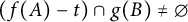 $\left ( f(A) - t\right ) \cap g(B)\neq \emptyset $
for
$\left ( f(A) - t\right ) \cap g(B)\neq \emptyset $
for
 $t\in D$
. This concludes implication (5.19).
$t\in D$
. This concludes implication (5.19).
Step 5. Show D contains an element of C: Recall as in Lemma 5.3 that
 $$ \begin{align*}D = \bar{B}\left( f(c_{1_A})-g(c_{1_B}), t_D\right)\end{align*} $$
and
 $$ \begin{align*}t_D=(1-2r)s_ft_{1_A}+s_gt_{1_B}-s_gh_{1_B}.\end{align*} $$
Lemma 5.4 Let
 $\alpha $
and
$\alpha $
and
 $\lambda $
be elements of
$\lambda $
be elements of
 $\mathcal {R}$
. Then,
$\mathcal {R}$
. Then,
 $$ \begin{align*}D\cap C\neq \emptyset.\end{align*} $$
Proof We will show that the center of the disc D lies inside the closed disc
 $S_\emptyset =\bar {B}(0,1)$
, and the radius
$S_\emptyset =\bar {B}(0,1)$
, and the radius
 $t_D$
is larger than
$t_D$
is larger than
 $2h_\emptyset $
, so D contains a disc of radius
$2h_\emptyset $
, so D contains a disc of radius
 $h_\emptyset $
inside
$h_\emptyset $
inside
 $S_\emptyset $
. Since this disc ball is contained in
$S_\emptyset $
. Since this disc ball is contained in
 $S_\emptyset $
, it must contain a point in C by definition of
$S_\emptyset $
, it must contain a point in C by definition of
 $h_\emptyset $
. From this, we conclude that D contains a point in C.
$h_\emptyset $
. From this, we conclude that D contains a point in C.
We proceed by first analyzing the center and radius of D.
The center of D is
 $f(c_{1_A})-g(c_{1_B})$
. A consequence of the choice of the sets
$f(c_{1_A})-g(c_{1_B})$
. A consequence of the choice of the sets
 $S_{1_A}$
and
$S_{1_A}$
and
 $S_{1_B}$
is that it sufficiently minimizes the distance between
$S_{1_B}$
is that it sufficiently minimizes the distance between
 $f(c_{1_A})$
and
$f(c_{1_A})$
and
 $g(c_{1_B})$
. Recall that, by assumption,
$g(c_{1_B})$
. Recall that, by assumption,
 $S_{1_A}$
,
$S_{1_A}$
,
 $S_{1_B}$
are both contained in
$S_{1_B}$
are both contained in
 $\bar {B}\left (0,\frac {1}{2}\right )$
. We can actually take a larger – though uglier – ball, and in this proof, we will suppose that
$\bar {B}\left (0,\frac {1}{2}\right )$
. We can actually take a larger – though uglier – ball, and in this proof, we will suppose that
 $S_{1_A}$
,
$S_{1_A}$
,
 $S_{1_B}$
are contained inside the ball
$S_{1_B}$
are contained inside the ball
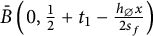 $\bar {B}\left (0,\frac {1}{2}+t_1-\frac {h_\emptyset x}{2s_f}\right )$
, where
$\bar {B}\left (0,\frac {1}{2}+t_1-\frac {h_\emptyset x}{2s_f}\right )$
, where
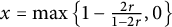 $x=\max \left \{1-\frac {2r}{1-2r},0\right \}$
.
$x=\max \left \{1-\frac {2r}{1-2r},0\right \}$
.
Note:
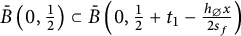 $\bar {B}\left (0,\frac {1}{2}\right )\subset \bar {B}\left ( 0,\frac {1}{2}+t_1-\frac {h_\emptyset x}{2s_f}\right )$
. This can be seen by combining (5.15) and (5.1):
$\bar {B}\left (0,\frac {1}{2}\right )\subset \bar {B}\left ( 0,\frac {1}{2}+t_1-\frac {h_\emptyset x}{2s_f}\right )$
. This can be seen by combining (5.15) and (5.1):
 $$ \begin{align*} \frac{s_g}{s_f}\frac{2}{1-2r} &\leq \frac{t_1}{h_\emptyset}. \end{align*} $$
Rearranging then gives
 $$ \begin{align*} h_\emptyset \frac{s_g}{s_f}\frac{2}{1-2r} &\leq t_1. \end{align*} $$
Because
 $$ \begin{align*} x &<1, & \frac{1}{2} &< s_g, & 1 &< \frac{2}{1-2r}, \end{align*} $$
we can combine the above inequalities to see
 $$ \begin{align*} h_\emptyset \frac{x}{2s_f} < h_\emptyset \frac{s_g}{s_f}\frac{2}{1-2r} < t_1. \end{align*} $$
Returning to our analysis of the center
 $f(c_{1_A})-g(c_{1_B})$
, observe that the centers of
$f(c_{1_A})-g(c_{1_B})$
, observe that the centers of
 $c_{1_A}$
,
$c_{1_A}$
,
 $c_{1_B}$
of
$c_{1_B}$
of
 $S_{1_A}$
,
$S_{1_A}$
,
 $S_{1_B}$
satisfy
$S_{1_B}$
satisfy
 $$ \begin{align*}\|c_{1_A}\|\leq \frac{1}{2}-\frac{h_\emptyset x}{2s_f} \quad \text{and}\quad \|c_{1_B}\|\leq \frac{1}{2}-\frac{h_\emptyset x}{2s_f}.\end{align*} $$
Because f, respectively g, rotates and scales by
 $s_f\leq 1$
, respectively
$s_f\leq 1$
, respectively
 $s_g\leq 1$
, we know
$s_g\leq 1$
, we know
 $$ \begin{align*}\|f(c_{1_A})\|\leq \frac{1}{2}s_f -\frac{h_\emptyset x}{2} \quad \text{and}\quad \|g(c_{1_B})\|\leq \frac{1}{2}s_g-\frac{h_\emptyset xs_g}{2s_f} \leq \frac{1}{2}s_g-\frac{h_\emptyset x}{2}.\end{align*} $$
Thus,
 $$ \begin{align} \|f(c_{1_A})-g(c_{1_B})\|\leq \frac{1}{2}(s_f+s_g) - h_\emptyset x \leq 1-h_\emptyset x. \end{align} $$
where the last inequality is from maximizing
 $s_f+s_g = \sqrt {\alpha ^2+\lambda ^2}+\sqrt {\alpha ^2+(1-\lambda )^2}$
on
$s_f+s_g = \sqrt {\alpha ^2+\lambda ^2}+\sqrt {\alpha ^2+(1-\lambda )^2}$
on
 $\bar {\mathcal {R}}$
, and the center of D,
$\bar {\mathcal {R}}$
, and the center of D,
 $f(c_{1_A})-g(c_{1_B})$
, is contained in
$f(c_{1_A})-g(c_{1_B})$
, is contained in
 $S_\emptyset $
.
$S_\emptyset $
.
Next, we analyze the radius of D. Observe that
 $$ \begin{align} t_D &= (1-2r)s_ft_{1_A} + s_gt_{1_B}-s_gh_{1_B} & \nonumber\\ & \geq \left( (1-2r)s_f + s_g \right) t_1 -2s_gh_\emptyset & t_1\leq t_{1_A},t_{1_B}, \text{ and } h_{1_B}\le 2h_\emptyset \text{ by (5.4)} \nonumber\\ &= h_\emptyset\left[ \left( (1-2r)s_f+s_g \right)\frac{t_1}{h_\emptyset} -2s_g \right] \nonumber\\ &\geq h_\emptyset\left[ \left( (1-2r)s_f + s_g\right) \frac{s_g}{s_f}\frac{2}{(1-2r)}-2s_g\right] & \text{ applying (5.20)} \nonumber\\ &= h_\emptyset \frac{s_g^2}{s_f} \frac{2}{(1-2r)} \nonumber\\ &= 2h_\emptyset \frac{s_g^2}{s_f} + 2h_\emptyset \frac{s_g^2}{s_f} \frac{2r}{(1-2r)}. & \end{align} $$
Claim:
 $\frac {s_g^2}{s_f} = \frac {\alpha ^2+(1-\lambda )^2}{\sqrt {\alpha ^2+\lambda ^2}}$
is minimized when
$\frac {s_g^2}{s_f} = \frac {\alpha ^2+(1-\lambda )^2}{\sqrt {\alpha ^2+\lambda ^2}}$
is minimized when
 $\alpha =0$
,
$\alpha =0$
,
 $\lambda =\frac {1}{2}$
in
$\lambda =\frac {1}{2}$
in
 $\bar {\mathcal {R}}$
with minimum value
$\bar {\mathcal {R}}$
with minimum value
 $\frac {1}{2}$
.
$\frac {1}{2}$
.
Then, (5.23) becomes
 $$ \begin{align} \qquad\qquad\quad\qquad t_D &\geq 2h_\emptyset \frac{s_g^2}{s_f} + 2h_\emptyset \frac{s_g^2}{s_f} \frac{2r}{(1-2r)} &\nonumber \\ &\geq h_\emptyset + h_\emptyset \frac{2r}{1-2r} \\ &> h_\emptyset. \nonumber \end{align} $$
Now if
 $D\subseteq S_\emptyset $
, then D is itself a ball of radius larger than
$D\subseteq S_\emptyset $
, then D is itself a ball of radius larger than
 $h_\emptyset $
by (5.24), so
$h_\emptyset $
by (5.24), so
 $D\subset S_\emptyset $
contains a point
$D\subset S_\emptyset $
contains a point
 $c\in C$
.
$c\in C$
.
If
 $D\not \subseteq S_\emptyset $
, then it must be the case that
$D\not \subseteq S_\emptyset $
, then it must be the case that
 $|f(c_{1_A}) - g(c_{1_B}) + t_D|>1$
, and we will use the lower bound on the radius (5.24) and upper bound on the norm of the center (5.22) below.
$|f(c_{1_A}) - g(c_{1_B}) + t_D|>1$
, and we will use the lower bound on the radius (5.24) and upper bound on the norm of the center (5.22) below.
If
 $$ \begin{align*} \left|\|f(c_{1_A})-g(c_{1_B})\|_2 - t_D\right| \le 1- 2h_\emptyset, \end{align*} $$
then it follows that the disk
 $D=\bar {B}\left ( f(c_{1_A})-g(c_{1_B}),t_D\right )$
intersects
$D=\bar {B}\left ( f(c_{1_A})-g(c_{1_B}),t_D\right )$
intersects
 $S_\emptyset =\bar {B}(0,1)$
in such a way that the intersection contains a ball of radius
$S_\emptyset =\bar {B}(0,1)$
in such a way that the intersection contains a ball of radius
 $h_\emptyset $
.
$h_\emptyset $
.
Hence, it remains to show that
 $$ \begin{align} 1+t_D -2h_\emptyset- \|f(c_{1_A})-g(c_{1_B})\|_2 \geq 0. \end{align} $$
Indeed,
 $$ \begin{align*} 1+t_D -2h_\emptyset- \|f(c_{1_A})-g(c_{1_B})\|_2 &\geq 1+\left( h_\emptyset + h_\emptyset\frac{2r}{1-2r}\right) -2h_\emptyset - \left(1-h_\emptyset x\right) \\ &= h_\emptyset \left( \frac{2r}{1-2r} - 1\right) +h_\emptyset x \\ &\geq 0, \end{align*} $$
because
 $0<r<\frac {1}{2}$
and
$0<r<\frac {1}{2}$
and
 $x = \max \left \{1-\frac {2r}{1-2r},0\right \}$
. This is where our choice of x in the radius comes from.
$x = \max \left \{1-\frac {2r}{1-2r},0\right \}$
. This is where our choice of x in the radius comes from.
Thus, (5.25) is confirmed, and we conclude
 $D\cap S_\emptyset $
contains a ball of radius
$D\cap S_\emptyset $
contains a ball of radius
 $h_\emptyset $
. This ball of radius
$h_\emptyset $
. This ball of radius
 $h_\emptyset $
is contained in
$h_\emptyset $
is contained in
 $S_\emptyset $
, so it must contain a point in C by definition of
$S_\emptyset $
, so it must contain a point in C by definition of
 $h_\emptyset $
. Therefore, D contains a point in C.
$h_\emptyset $
. Therefore, D contains a point in C.
Combining Lemmas 5.3 and 5.4, the disk D is contained in
 $f(A)-g(B)$
and
$f(A)-g(B)$
and
 $D\cap C\neq \emptyset $
. This implies that there is an element of c in
$D\cap C\neq \emptyset $
. This implies that there is an element of c in
 $f(A)-g(B)$
.
$f(A)-g(B)$
.
6 Examples
6.1 Convex combinations in
$\mathbb {R}^d$

As Yavicoli illustrated in [Reference Yavicoli40], compact sets can be constructed using a system of balls, including self-similar sets where each generation of children are equally spaced in a grid. For such an example, the existence of an arithmetic progression is immediate regardless of the thickness as there will be three children in a row (or column) all containing the exact same points through self-similarity.
In what follows, we provide an example of a compact set using the infinity norm
 $\|\cdot \|_\infty $
which contains a
$\|\cdot \|_\infty $
which contains a
 $3$
-term arithmetic progression that is not obvious. Note, one can modify this example to work with other norms by re-arranging the norm balls to their respective optimal packing shape, such as a hexagonal packing arrangement for
$3$
-term arithmetic progression that is not obvious. Note, one can modify this example to work with other norms by re-arranging the norm balls to their respective optimal packing shape, such as a hexagonal packing arrangement for
 $\|\cdot \|_2$
; this may introduce constants that could alter the stated thickness condition.
$\|\cdot \|_2$
; this may introduce constants that could alter the stated thickness condition.
We first construct a self-similar compact set C, and then we introduce randomness to the construction. Let
 $S_\emptyset = \bar {B}(0,1)$
be a ball in the infinity norm. Let
$S_\emptyset = \bar {B}(0,1)$
be a ball in the infinity norm. Let
 $n^2$
be the number of children in each generation and
$n^2$
be the number of children in each generation and
 $\rho $
be the fixed radius for all of the first-generation children. We take the
$\rho $
be the fixed radius for all of the first-generation children. We take the
 $n^2$
children to be equidistant in an
$n^2$
children to be equidistant in an
 $n\times n$
grid, where the children in a generation are all distance d apart from each other and distance
$n\times n$
grid, where the children in a generation are all distance d apart from each other and distance
 $d/2$
away from the boundary of
$d/2$
away from the boundary of
 $\bar {B}(0,1)$
, as shown in Figure 4.
$\bar {B}(0,1)$
, as shown in Figure 4.
Parent square
 $S_\emptyset $
and first-generation children of radius
$S_\emptyset $
and first-generation children of radius
 $\rho $
for self-similar compact set C in the infinity norm
$\rho $
for self-similar compact set C in the infinity norm
 $\|\cdot \|_\infty $
.
$\|\cdot \|_\infty $
.

Note that we must have
 $$ \begin{align*}2\rho n+nd=2\end{align*} $$
because
 $S_\emptyset =B(0,1)$
. A compact set such as this can be described by an iterated function system
$S_\emptyset =B(0,1)$
. A compact set such as this can be described by an iterated function system
 $f_{i}(x) = \rho x + t_{i}$
where the
$f_{i}(x) = \rho x + t_{i}$
where the
 $t_{i}$
are the equidistributed centers of each child for
$t_{i}$
are the equidistributed centers of each child for
 $1\leq i\leq n^2$
. By construction,
$1\leq i\leq n^2$
. By construction,
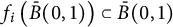 $f_i\left ( \bar {B}(0,1)\right ) \subset \bar {B}(0,1)$
for all
$f_i\left ( \bar {B}(0,1)\right ) \subset \bar {B}(0,1)$
for all
 $1\leq i\leq n^2$
. We label these sets
$1\leq i\leq n^2$
. We label these sets
 $S_{i_1\cdots i_{j}} = f_{i_1}\cdots f_{i_j}(\bar {B}(0,1))$
.
$S_{i_1\cdots i_{j}} = f_{i_1}\cdots f_{i_j}(\bar {B}(0,1))$
.
As previously mentioned, such a self-similar set has “obvious”
 $3$
-term arithmetic progressions and is a trivial illustration of our proof. However, we can introduce randomness to this IFS to make the existence of a
$3$
-term arithmetic progressions and is a trivial illustration of our proof. However, we can introduce randomness to this IFS to make the existence of a
 $3$
-term arithmetic progression nontrivial.
$3$
-term arithmetic progression nontrivial.
We modify our previous construction by starting with
 $S_\emptyset = \bar {B}(0,1)$
and let
$S_\emptyset = \bar {B}(0,1)$
and let
 $f_{i}^k = \rho x + \tilde {t}_{i}^k$
, where
$f_{i}^k = \rho x + \tilde {t}_{i}^k$
, where
 $\tilde {t}_{i}^k = t_{i} + u_{i}^k$
such that
$\tilde {t}_{i}^k = t_{i} + u_{i}^k$
such that
 $|u_{i}^k|< \frac {d}{2}$
is random for all
$|u_{i}^k|< \frac {d}{2}$
is random for all
 $1\leq i\leq n^2$
and
$1\leq i\leq n^2$
and
 $k\geq 1$
. Even with the added randomness, we see that C is
$k\geq 1$
. Even with the added randomness, we see that C is
 $(2\rho +d)$
-uniformly dense in Figure 5.
$(2\rho +d)$
-uniformly dense in Figure 5.
Parent square
 $S_\emptyset $
and first-generation children of radius
$S_\emptyset $
and first-generation children of radius
 $\rho $
for randomly perturbed self-similar compact set C in the infinity norm
$\rho $
for randomly perturbed self-similar compact set C in the infinity norm
 $\|\cdot \|_\infty $
.
$\|\cdot \|_\infty $
.

Figure 5: Long description
At the top-left is a square with a solid outline, labeled d divided by 2 at its upper left. To its right are two more squares, forming the top row of three. The middle and bottom rows each contain three squares, aligned vertically. Dotted outlines surround each square, indicating possible perturbations. The distance between adjacent squares is labeled d, and a horizontal dashed line labeled rho appears inside the top-center square. Ellipses to the right and below each row suggest continuation. The arrangement illustrates the parent square and its first-generation children in a self-similar compact set under the infinity norm.
Then, by construction
 $$ \begin{align*}\max_{x\in S_\emptyset} \operatorname{\mathrm{dist}}\left( x,\bigcup_{i} S_i^k \right)\leq d,\end{align*} $$
because each
 $S_i^k$
is a maximum distance d apart. As this is repeated at each level but scaled to
$S_i^k$
is a maximum distance d apart. As this is repeated at each level but scaled to
 $\rho $
, in general, we have
$\rho $
, in general, we have
 $$ \begin{align*}\max_{x\in S_I^K} \operatorname{\mathrm{dist}}\left( x,\bigcup_{i} S_{I,i}^{K,k} \right)\leq \rho^{\ell(I)} d.\end{align*} $$
Consequently,
 $$ \begin{align*}h_I(C) \leq d\rho^{\ell(I)} + d\rho^{\ell(I)+1}+ d\rho^{\ell(I)+2}+\cdots = \frac{d\rho^{\ell(I)}}{1-\rho}.\end{align*} $$
By construction,
 $$ \begin{align*}\min_i \operatorname{\mathrm{rad}} (S_{I,i}^{K,k}) = \rho ^{\ell(I)+1}.\end{align*} $$
This gives a lower bound on the thickness of our compact set:
 $$ \begin{align} \tau\left( C,\{S_I\}\right)\geq \frac{\rho(1-\rho)}{d}. \end{align} $$
Corollary 2.9 then gives the existence of
 $3$
APs in these compact sets C when
$3$
APs in these compact sets C when
 $0 < 2\rho + d < \frac {1}{2}$
and
$0 < 2\rho + d < \frac {1}{2}$
and
 $\tau \left ( C,\{S_I\}\right ) \geq \frac {2}{1-4\rho -2d}$
. In particular, we can take
$\tau \left ( C,\{S_I\}\right ) \geq \frac {2}{1-4\rho -2d}$
. In particular, we can take
 $n=10$
,
$n=10$
,
 $\rho =0.095$
, and
$\rho =0.095$
, and
 $d=0.01$
. Then, by inequality (6.1),
$d=0.01$
. Then, by inequality (6.1),
 $$ \begin{align*}\tau\left( C,\{S_I\}\right) \geq \frac{0.095(1-0.095)}{0.01} = 8.5975,\end{align*} $$
which is larger than the Corollary 2.9 requirement of
 $$ \begin{align*}\frac{2}{1-4\rho-2d} = \frac{2}{1-4\cdot 0.095 -2\cdot 0.1} = 3.\bar{3}.\end{align*} $$
Thus, C contains a
 $3$
-term arithmetic progression. In fact, we can apply Theorem 2.8 to see that C contains a homothetic copy of all convex combinations of the form
$3$
-term arithmetic progression. In fact, we can apply Theorem 2.8 to see that C contains a homothetic copy of all convex combinations of the form
 $\{a,\lambda a+(1-\lambda )b, b\}$
for
$\{a,\lambda a+(1-\lambda )b, b\}$
for
 $\lambda \in [0.27938814,0.5]$
.
$\lambda \in [0.27938814,0.5]$
.
Other n,
 $\rho $
, and d values can be chosen to construct a different C which also contain
$\rho $
, and d values can be chosen to construct a different C which also contain
 $3$
-term arithmetic progressions or convex combinations.
$3$
-term arithmetic progressions or convex combinations.
Additional examples can be constructed using Yavicoli’s method [Reference Yavicoli40, Section 4.1, Lemma 7].
6.2 Triangles in
$\mathbb {R}^2$

We now construct a compact set
 $C\in \mathbb {R}^2$
using the Euclidean norm to which we can apply Theorem 2.12 and Corollary 2.14 to get the existence of nondegenerate
$C\in \mathbb {R}^2$
using the Euclidean norm to which we can apply Theorem 2.12 and Corollary 2.14 to get the existence of nondegenerate
 $3$
-point configurations. Theorem 2.8 and Corollary 2.9 will also apply and give the existence of linear configurations.
$3$
-point configurations. Theorem 2.8 and Corollary 2.9 will also apply and give the existence of linear configurations.
We begin by taking the best-known packing of
 $55$
congruent circles inside the circle
$55$
congruent circles inside the circle
 $S_\emptyset =\bar {B}(0,1)$
, as determined by [Reference Graham, Lubachevsky, Nurmela and Östergård13] and illustrated in Figure 6.
$S_\emptyset =\bar {B}(0,1)$
, as determined by [Reference Graham, Lubachevsky, Nurmela and Östergård13] and illustrated in Figure 6.
Best known packing [Reference Graham, Lubachevsky, Nurmela and Östergård13] of
 $55$
congruent circles in
$55$
congruent circles in
 $\bar {B}(0,1)$
.
$\bar {B}(0,1)$
.

Figure 6: Long description
At the center is a single small circle. Surrounding this, five concentric layers of equal circles are arranged in a hexagonal close-packed structure, each tangent to its neighbors and the enclosing large circle. The outermost circles touch the boundary of the large circle, which is centered within a faint hexagonal grid that extends beyond the packing. The grid lines are visible but do not intersect the packed circles. The arrangement maximizes the number of non-overlapping circles within the boundary.
Observe that these circles, call them
 $S_1, S_2, \cdots S_{55}$
, are in a hexagonal packing arrangement, the most dense packing arrangement for circles. This forces all the congruent circles, which will become our first-generation children, to have radii
$S_1, S_2, \cdots S_{55}$
, are in a hexagonal packing arrangement, the most dense packing arrangement for circles. This forces all the congruent circles, which will become our first-generation children, to have radii
 $\rho \approx 0.12179$
. At this moment, notice that
$\rho \approx 0.12179$
. At this moment, notice that
 $$ \begin{align*} \max_{x\in \bar{B}(0,1)}\operatorname{\mathrm{dist}}\left( x,\cup_1^{55} S_i\right)> \rho, \end{align*} $$
and this would cause our thickness to be less than or equal to
 $1$
. Hence, we add
$1$
. Hence, we add
 $30$
additional congruent circles
$30$
additional congruent circles
 $S_{56},\ldots ,S_{85}$
around the edges, shown in Figure 7. This provides the better bound
$S_{56},\ldots ,S_{85}$
around the edges, shown in Figure 7. This provides the better bound
 $$ \begin{align} \max_{x\in \bar{B}(0,1)}\operatorname{\mathrm{dist}}\left( x,\cup_1^{85} S_i\right) = \frac{2-\sqrt{3}}{\sqrt{3}}\rho. \end{align} $$
Best known packing of
 $55$
congruent circles in
$55$
congruent circles in
 $\bar {B}(0,1)$
with congruent circles added to minimize
$\bar {B}(0,1)$
with congruent circles added to minimize
 $\max _{x\in \bar {B}(0,1)}\operatorname {\mathrm {dist}}(x,C)$
.
$\max _{x\in \bar {B}(0,1)}\operatorname {\mathrm {dist}}(x,C)$
.

Figure 7: Long description
At the center is a large black-outlined circle. Inside, 55 smaller black circles of equal size are tightly packed in a hexagonal lattice, filling the interior with minimal gaps. Along the perimeter, a ring of congruent red circles is arranged so that each red circle overlaps the boundary of the large circle, with their centers lying just outside the main circle. The red circles are evenly spaced and partially overlap each other. The background consists of a faint, regular hexagonal grid extending beyond the main circle. No text labels are present. The arrangement demonstrates optimal packing and boundary minimization.
Using this structure, we can construct the compact set
 $C\subset \mathbb {R}^d$
by translating, scaling by
$C\subset \mathbb {R}^d$
by translating, scaling by
 $\rho $
, (and optionally rotating) a copy of Figure 7 into each
$\rho $
, (and optionally rotating) a copy of Figure 7 into each
 $S_i$
and repeating at every level of the construction. The resulting compact set C generated by
$S_i$
and repeating at every level of the construction. The resulting compact set C generated by
 $\{S_I\}_I$
is
$\{S_I\}_I$
is
 $\frac {2+\sqrt {3}}{\sqrt {3}}\rho $
-uniformly dense, or
$\frac {2+\sqrt {3}}{\sqrt {3}}\rho $
-uniformly dense, or
 $0.26243$
-uniformly dense. Using self-similarity with inequality (6.2) gives
$0.26243$
-uniformly dense. Using self-similarity with inequality (6.2) gives
 $$ \begin{align*} \max_{x\in S_I}\operatorname{\mathrm{dist}}(x,C) \leq \frac{2-\sqrt{3}}{\sqrt{3}} \frac{\rho^{\ell(I)}}{1+\rho}. \end{align*} $$
Because
 $$ \begin{align*} \min_i\operatorname{\mathrm{rad}}(S_{I,i}) = \rho^{\ell(I)+1}, \end{align*} $$
we know
 $$ \begin{align*} \tau\left( C,\{S_I\}\right) \geq \frac{\rho(1+\rho)}{\frac{2-\sqrt{3}}{\sqrt{3}} \rho}\approx 7.25137. \end{align*} $$
While this result establishes the existence of compact sets in
 $\mathbb {R}^2$
using the Euclidean norm of sufficient thickness, it does not satisfy the requirement in Theorem 2.12 that there are two first-generation children that are disjoint from the others. We remedy this by constructing a new compact set
$\mathbb {R}^2$
using the Euclidean norm of sufficient thickness, it does not satisfy the requirement in Theorem 2.12 that there are two first-generation children that are disjoint from the others. We remedy this by constructing a new compact set
 $\tilde {C}$
from the compact set C generated by
$\tilde {C}$
from the compact set C generated by
 $\{S_I\}_I$
by taking two first-generation balls
$\{S_I\}_I$
by taking two first-generation balls
 $S_{1_A}$
,
$S_{1_A}$
,
 $S_{1_B}$
in
$S_{1_B}$
in
 $\bar {B}(0,\frac {1}{2})$
, as illustrated in Figure 8, and scaling them, and all their children, by a factor of
$\bar {B}(0,\frac {1}{2})$
, as illustrated in Figure 8, and scaling them, and all their children, by a factor of
 $\gamma $
for
$\gamma $
for
 $0<\gamma <1$
; e.g.,
$0<\gamma <1$
; e.g.,
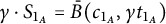 $\gamma \cdot S_{1_A} = \bar {B}(c_{1_A},\gamma t_{1_A})$
.
$\gamma \cdot S_{1_A} = \bar {B}(c_{1_A},\gamma t_{1_A})$
.
Modifying construction so two congruent circles in
 $\bar {B}(0,\frac {1}{2})$
are disjoint.
$\bar {B}(0,\frac {1}{2})$
are disjoint.

Figure 8: Long description
At the center are two adjacent circles outlined in red. Surrounding them are multiple layers of congruent black circles, each layer forming a ring that increases in radius. All circles are contained within a large black circle. The arrangement is overlaid on a faint hexagonal grid, with the circles positioned to fit within the grid's cells. The red circles are the only ones not overlapping, while the black circles in outer layers overlap at their boundaries, especially near the perimeter.
We then construct the compact set
 $\tilde {C}$
as before with the new generating system of balls
$\tilde {C}$
as before with the new generating system of balls
 $\{\tilde {S}_I\}$
. This then shifts inequality (6.2) to become
$\{\tilde {S}_I\}$
. This then shifts inequality (6.2) to become
 $$ \begin{align*} \max_{x\in\bar{B}(0,1)}\operatorname{\mathrm{dist}}\left( x,\cup_1^{81}\tilde{S}_i\right) \leq \frac{2-\sqrt{3}}{\sqrt{3}}\rho +(1-\gamma)\rho = \left(\frac{2}{\sqrt{3}}-\gamma\right)\rho. \end{align*} $$
For words
 $I\neq \emptyset $
and not starting with
$I\neq \emptyset $
and not starting with
 $1_A$
or
$1_A$
or
 $1_B$
, we still have
$1_B$
, we still have
 $$ \begin{align*} \max_{x\in \tilde{S}_I}\operatorname{\mathrm{dist}}(x,\tilde{C}) \leq \frac{2-\sqrt{3}}{\sqrt{3}} \frac{\rho^{\ell(I)}}{1+\rho} \quad\text{and}\quad \min_i\operatorname{\mathrm{rad}}(\tilde{S}_{I,i}) = \rho^{\ell(I)+1}. \end{align*} $$
However, for words
 $I\neq \emptyset $
starting with
$I\neq \emptyset $
starting with
 $1_A$
or
$1_A$
or
 $1_B$
,
$1_B$
,
 $$ \begin{align*} \max_{x\in \tilde{S}_I}\operatorname{\mathrm{dist}}(x,\tilde{C}) \leq \gamma \frac{2-\sqrt{3}}{\sqrt{3}} \frac{\rho^{\ell(I)}}{1+\rho} \quad\text{and}\quad \min_i\operatorname{\mathrm{rad}}(\tilde{S}_{I,i})=\gamma\rho^{\ell(I)+1}, \end{align*} $$
and lastly for
 $I=\emptyset $
,
$I=\emptyset $
,
 $$ \begin{align*} \max_{x\in \tilde{S}_\emptyset}\operatorname{\mathrm{dist}}(x,\tilde{C}) \leq \left(1-\gamma\right)\rho + \frac{2-\sqrt{3}}{\sqrt{3}} \frac{\rho}{1+\rho} \quad\text{and}\quad \min_i \operatorname{\mathrm{rad}}(\tilde{S}_i) = \gamma\rho. \end{align*} $$
Consequently, the thickness of
 $\tilde {C}$
generated by this system is
$\tilde {C}$
generated by this system is
 $$ \begin{align*} \tau\left( \tilde{C},\{\tilde{S}_I\}\right) \geq \frac{\gamma\rho}{\left(1-\gamma\right)\rho + \frac{2-\sqrt{3}}{\sqrt{3}} \frac{\rho}{1+\rho}}. \end{align*} $$
In the case of
 $\gamma =0.99999$
,
$\gamma =0.99999$
,
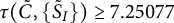 $\tau (\tilde {C},\{\tilde {S}_I\}) \geq 7.25077$
, so
$\tau (\tilde {C},\{\tilde {S}_I\}) \geq 7.25077$
, so
 $$ \begin{align*} \tau(\tilde{C},\{\tilde{S}_I\}) \geq \sqrt{ \frac{\alpha^2+(1-\lambda)^2}{\alpha^2+\lambda^2} }\cdot\frac{2}{1-2\cdot 0.262421} \end{align*} $$
for all
 $(\alpha ,\lambda )\in \mathcal {R}\cap (0,\sqrt {3}/2]\times [3/10,1/2]$
. Thus, by Theorem 2.12,
$(\alpha ,\lambda )\in \mathcal {R}\cap (0,\sqrt {3}/2]\times [3/10,1/2]$
. Thus, by Theorem 2.12,
 $\tilde {C}$
contains a similar triangle to
$\tilde {C}$
contains a similar triangle to
 $\mathcal {T}(\alpha ,\lambda )$
for all
$\mathcal {T}(\alpha ,\lambda )$
for all
 $(\alpha ,\lambda )\in \mathcal {R}\cap (0,\sqrt {3}/2]\times [3/10,1/2]$
. In particular,
$(\alpha ,\lambda )\in \mathcal {R}\cap (0,\sqrt {3}/2]\times [3/10,1/2]$
. In particular,
 $\tilde {C}$
contains a similar copy of an equilateral triangle.
$\tilde {C}$
contains a similar copy of an equilateral triangle.
Remark 6.1 A similar construction could be used for the optimal packing of
 $31$
congruent circles in
$31$
congruent circles in
 $\bar {B}(0,1)$
, which also utilizes a hexagonal packing arrangement. This thickness would naturally be a little smaller than our example.
$\bar {B}(0,1)$
, which also utilizes a hexagonal packing arrangement. This thickness would naturally be a little smaller than our example.
Appendix
In this appendix, we consider a special case in which Lemma 3.5 can be improved by a factor of
 $1/2$
and state the main results with a slightly improved thickness threshold.
$1/2$
and state the main results with a slightly improved thickness threshold.
Consider a compact set
 $C\subset \mathbb {R}$
with the open intervals
$C\subset \mathbb {R}$
with the open intervals
 $(G_n)$
making up
$(G_n)$
making up
 $\mathbb {R}\setminus C$
ordered by decreasing length. Suppose additionally that
$\mathbb {R}\setminus C$
ordered by decreasing length. Suppose additionally that
 $\tau (C)\geq 1$
. Thus, when we remove
$\tau (C)\geq 1$
. Thus, when we remove
 $G_1$
from C, we are left with the two intervals
$G_1$
from C, we are left with the two intervals
 $L_1$
and
$L_1$
and
 $R_1$
. Let
$R_1$
. Let
 $A=L_1\cap C$
or
$A=L_1\cap C$
or
 $A=R_1\cap C$
, so A is a compact set with the open intervals
$A=R_1\cap C$
, so A is a compact set with the open intervals
 $(G_n')$
making up
$(G_n')$
making up
 $\mathbb {R}\setminus A$
. Observe that the
$\mathbb {R}\setminus A$
. Observe that the
 $(G_n')$
are a subsequence of the
$(G_n')$
are a subsequence of the
 $(G_n)$
. Then
$(G_n)$
. Then
 $$ \begin{align*} \tau(A) = \inf_{n\in\mathbb{N}} \frac{ \min\{|L_n'|, |R_n'|\} }{|G_n'|} \geq \inf_{n\in\mathbb{N}}\frac{ \min\{|L_n|, |R_n|\} }{|G_n|} = \tau(C). \end{align*} $$
Thus, in
 $\mathbb {R}$
, we can construct subsets A of C such that
$\mathbb {R}$
, we can construct subsets A of C such that
 $$ \begin{align*}\tau(A)\geq \tau(C).\end{align*} $$
A direct consequence of this is that if
 $C\subset \mathbb {R}$
satisfies
$C\subset \mathbb {R}$
satisfies
 $\tau (C)\geq 1$
then, at minimum, C contains countably many distinctFootnote
1
$\tau (C)\geq 1$
then, at minimum, C contains countably many distinctFootnote
1
 $3$
-term arithmetic progressions as we can apply Proposition 1.1 to
$3$
-term arithmetic progressions as we can apply Proposition 1.1 to
 $C\cap L_n$
for all n.
$C\cap L_n$
for all n.
On the other hand, every time Theorem 2.8 is applied to some
 $C\subset \mathbb {R}^d$
with
$C\subset \mathbb {R}^d$
with
 $A=C\cap S_i$
, the lower bound on the thickness decreases proportionally by
$A=C\cap S_i$
, the lower bound on the thickness decreases proportionally by
 $\frac {1}{2}$
,
$\frac {1}{2}$
,
 $$ \begin{align*}\tau\left( A,\{S_I\}\right) \geq \frac{1}{2}\tau\left( C,\{S_I\}\right).\end{align*} $$
Hence, Theorem 2.8 can only be applied a finite number of times, and we cannot quantify the number of
 $3$
-term arithmetic progressions beyond the existence of one
$3$
-term arithmetic progressions beyond the existence of one
 $3$
AP.
$3$
AP.
In order to have a compact set
 $C\subset \mathbb {R}^d$
and a subset
$C\subset \mathbb {R}^d$
and a subset
 $A=C\cap S_{1_A}$
satisfy the condition
$A=C\cap S_{1_A}$
satisfy the condition
 $\tau (A)\geq \tau (C)$
, we would need a constraint that forces
$\tau (A)\geq \tau (C)$
, we would need a constraint that forces
 $$ \begin{align*}\max_{x\in S_{1_A}}\operatorname{\mathrm{dist}}(x,C) = \max_{x\in S_{1_A}}\operatorname{\mathrm{dist}}(x,A).\end{align*} $$
One way to achieve this is as follows:
Lemma A.1 (An improvement for the thickness of a subset in case of a distance child)
Let C be a compact set in
 $(\mathbb {R}^d,\operatorname {\mathrm {dist}})$
generated by the system of balls
$(\mathbb {R}^d,\operatorname {\mathrm {dist}})$
generated by the system of balls
 $\{S_I\}_I$
. Suppose that there exists some
$\{S_I\}_I$
. Suppose that there exists some
 $1\leq \ell \leq k_\emptyset $
such that
$1\leq \ell \leq k_\emptyset $
such that
 $$ \begin{align} \max_{x\in S_{\ell}}\operatorname{\mathrm{dist}}(x,C) < \min_{\substack{1 \leq i\leq k_\emptyset\\i\neq \ell}}\operatorname{\mathrm{dist}} (S_i,S_\ell). \end{align} $$
Then,
 $$ \begin{align*}\tau\left( C\cap S_\ell, \{S_{\ell,I}\}\right) \geq \tau\left( C, \{S_I\}\right).\end{align*} $$
Proof Let everything be as above. By definition, there exists some
 $c\in C$
and
$c\in C$
and
 $y\in S_\ell $
such that
$y\in S_\ell $
such that
 $$ \begin{align*}\operatorname{\mathrm{dist}}(c,y) = \max_{x\in S_\ell} \operatorname{\mathrm{dist}}(x,C).\end{align*} $$
As
 $c\in C$
and
$c\in C$
and
 $S_i \cap S_j=\emptyset $
for all
$S_i \cap S_j=\emptyset $
for all
 $i\neq j$
, there exists exactly one
$i\neq j$
, there exists exactly one
 $S_i$
containing c. As
$S_i$
containing c. As
 $$ \begin{align*} \operatorname{\mathrm{dist}}(c,y) = \max_{x\in S_\ell} \operatorname{\mathrm{dist}}(x,C) <\min_{\substack{1 \leq i\leq k_\emptyset\\i\neq \ell}}\operatorname{\mathrm{dist}} (S_i,S_\ell). \end{align*} $$
we know
 $c\in S_\ell $
which means
$c\in S_\ell $
which means
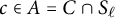 $c \in A=C\cap S_\ell $
. Thus
$c \in A=C\cap S_\ell $
. Thus
 $$ \begin{align*}\max_{x\in S_\ell}\operatorname{\mathrm{dist}}(x,C) = \max_{x\in S_\ell} \operatorname{\mathrm{dist}}(x,A).\end{align*} $$
This allows us to conclude
 $$ \begin{align*} \tau\left( A, \{S_{1_A,I}\}\right) &= \inf_{n\geq 1} \inf_{\substack{\ell(I)=n\\ I=\{1_A,\ldots\}}} \frac{\min_i \operatorname{\mathrm{rad}}(S_{I,i})}{\max_{x\in S_{I}} \operatorname{\mathrm{dist}}(x,A)} = \inf_{n\geq1} \inf_{\substack{\ell(I)=n\\I=\{1_A,\ldots\} }} \frac{\min_i \operatorname{\mathrm{rad}}(S_{I,i})}{\max_{x\in S_{I}} \operatorname{\mathrm{dist}}(x,C)} \\ &\geq \inf_{n\geq0} \inf_{\ell(I)=n} \frac{\min_i \operatorname{\mathrm{rad}}(S_{I,i})}{\max_{x\in S_I} \operatorname{\mathrm{dist}}(x,C)} =\tau\left( C, \{S_I\}\right). \end{align*} $$
Thus, in order to adapt the arguments of Theorem 2.8, we would need two distinct
 $\ell $
values,
$\ell $
values,
 $1_A$
and
$1_A$
and
 $1_B$
(see Remark 3.6 for why), satisfying inequality (A.1) to construct
$1_B$
(see Remark 3.6 for why), satisfying inequality (A.1) to construct
 $A= C\cap S_{1_A}$
and
$A= C\cap S_{1_A}$
and
 $B=C\cap S_{1_B}$
. Moreover, the inequalities (5.4) and Lemma 3.5 would be replaced by the following equations and inequalities:
$B=C\cap S_{1_B}$
. Moreover, the inequalities (5.4) and Lemma 3.5 would be replaced by the following equations and inequalities:
 $$ \begin{align*} h_{1_A,I}(A) = h_{1_A,I}(C) \quad\text{and}\quad h_{1_B,I}(B) = h_{1_B,I}(C) \end{align*} $$
and
 $$ \begin{align*} \tau\left( A, \{S_{1_A,I}\}\right) \geq \tau\left( C, \{S_I\}\right) \quad \text{and}\quad \tau\left( B, \{S_{1_B,I}\}\right) \geq \tau\left( C, \{S_I\}\right). \end{align*} $$
These new equations and inequalities will have a minor impact in the proof of Lemma 5.1 and a major impact in the proof of Lemma 5.2; in particular, to ensure that
 $t_D\geq h_\emptyset $
we are able to reduce the thickness constraint to
$t_D\geq h_\emptyset $
we are able to reduce the thickness constraint to
 $$ \begin{align*} \tau\left( C,\{S_I\}\right) \geq \frac{3(1-\lambda)}{2\lambda(1-2r)}. \end{align*} $$
Theorem A.2 Let C be a compact set in
 $(\mathbb {R}^d,\operatorname {\mathrm {dist}})$
generated by the system of balls
$(\mathbb {R}^d,\operatorname {\mathrm {dist}})$
generated by the system of balls
 $\{S_I\}_I$
such that C is r-uniformly dense where
$\{S_I\}_I$
such that C is r-uniformly dense where
 $ 0<r<\frac {1}{2}$
. Let
$ 0<r<\frac {1}{2}$
. Let
 $\lambda \in (0,\frac 12]$
, and suppose that
$\lambda \in (0,\frac 12]$
, and suppose that
 $$ \begin{align*}\tau\left( C,\{S_I\}\right) \geq \frac{3(1-\lambda)}{2\lambda(1-2r)}.\end{align*} $$
Suppose that there exist distinct first-generation children
 $S_{1_A}$
,
$S_{1_A}$
,
 $S_{1_B}$
such that
$S_{1_B}$
such that
 $$ \begin{align*} \max_{x\in S_{\ell}}\operatorname{\mathrm{dist}}(x,C) < \min_{\substack{1 \leq i\leq k_\emptyset\\i\neq \ell}}\operatorname{\mathrm{dist}} (S_i,S_\ell), \end{align*} $$
for
 $\ell =1_A,1_B$
. Then, C contains a
$\ell =1_A,1_B$
. Then, C contains a
 $3$
-point convex combination of the form
$3$
-point convex combination of the form
 $$ \begin{align*}\{a,\lambda a+(1-\lambda)b,b\}.\end{align*} $$
A similar argument can be made for Theorem 2.12, where we additionally take
 $x' = \max \left \{ \frac {7}{4}-\frac {3}{4(1-2r)},0 \right \}$
in place of
$x' = \max \left \{ \frac {7}{4}-\frac {3}{4(1-2r)},0 \right \}$
in place of
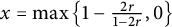 $x = \max \left \{1-\frac {2r}{1-2r},0\right \}$
.
$x = \max \left \{1-\frac {2r}{1-2r},0\right \}$
.
Theorem A.3 Let
 $\mathcal {T}$
denote the vertices of any triangle in
$\mathcal {T}$
denote the vertices of any triangle in
 $\mathbb {R}^2$
, and let
$\mathbb {R}^2$
, and let
 $\mathcal {T}(\alpha ,\lambda )$
be a triangle similar to
$\mathcal {T}(\alpha ,\lambda )$
be a triangle similar to
 $\mathcal {T}$
resulting from Lemma 2.11 for some
$\mathcal {T}$
resulting from Lemma 2.11 for some
 $\alpha $
,
$\alpha $
,
 $\lambda $
in
$\lambda $
in
 $\mathcal {R}$
. Let
$\mathcal {R}$
. Let
 $C\subset \mathbb {R}^2$
be a compact set generated by the system of balls
$C\subset \mathbb {R}^2$
be a compact set generated by the system of balls
 $\{S_I\}$
in the Euclidean norm such that C is r-uniformly dense for some
$\{S_I\}$
in the Euclidean norm such that C is r-uniformly dense for some
 $0<r<\frac {1}{2}$
. Suppose there exists distinct first-generation children
$0<r<\frac {1}{2}$
. Suppose there exists distinct first-generation children
 $S_{1_A}$
and
$S_{1_A}$
and
 $S_{1_B}$
,
$S_{1_B}$
,
 $1\leq 1_A<1_B\leq k_\emptyset $
, contained in
$1\leq 1_A<1_B\leq k_\emptyset $
, contained in
 $\bar {B}\left (0,\frac {1}{2}\right )$
such that
$\bar {B}\left (0,\frac {1}{2}\right )$
such that
 $$ \begin{align*} \max_{x\in S_{\ell}}\operatorname{\mathrm{dist}}(x,C) < \min_{\substack{1 \leq i\leq k_\emptyset\\i\neq \ell}}\operatorname{\mathrm{dist}} (S_i,S_\ell), \end{align*} $$
for
 $\ell =1_A,1_B$
. Further, suppose
$\ell =1_A,1_B$
. Further, suppose
 $$ \begin{align*}\tau\left( C,\{S_I\}\right) \geq \sqrt{\frac{\alpha^2+(1-\lambda)^2}{\alpha^2+\lambda^2}}\cdot \frac{3}{2(1-2r)},\end{align*} $$
then C contains the vertices of a similar copy of
 $\mathcal {T}$
.
$\mathcal {T}$
.
In order to guarantee the existence of countably many
 $3$
-term arithmetic progressions, we would need to apply Theorem A.2 at every level of the construction of
$3$
-term arithmetic progressions, we would need to apply Theorem A.2 at every level of the construction of
 $\{S_I\}$
; i.e., for all words I there exists at least two distinct
$\{S_I\}$
; i.e., for all words I there exists at least two distinct
 $\ell $
values such that
$\ell $
values such that
 $$ \begin{align*} \max_{x\in S_{I,\ell}}\operatorname{\mathrm{dist}}(x,C) < \min_{\substack{1 \leq i,j\leq k_I\\i\neq j}}\operatorname{\mathrm{dist}} (S_{I,i},S_{I,j}). \end{align*} $$
Acknowledgements
The authors thank Alex McDonald for illuminating conversations during the preparation of this article, as well as the anonymous referee for their valuable feedback.


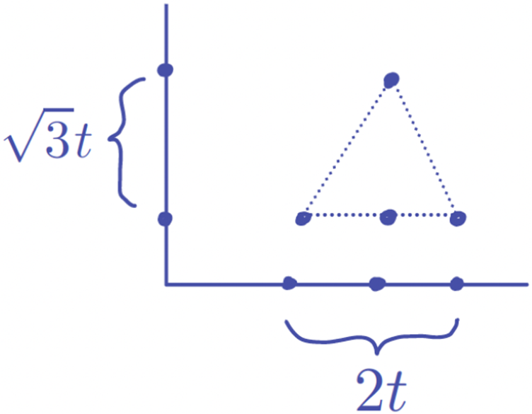


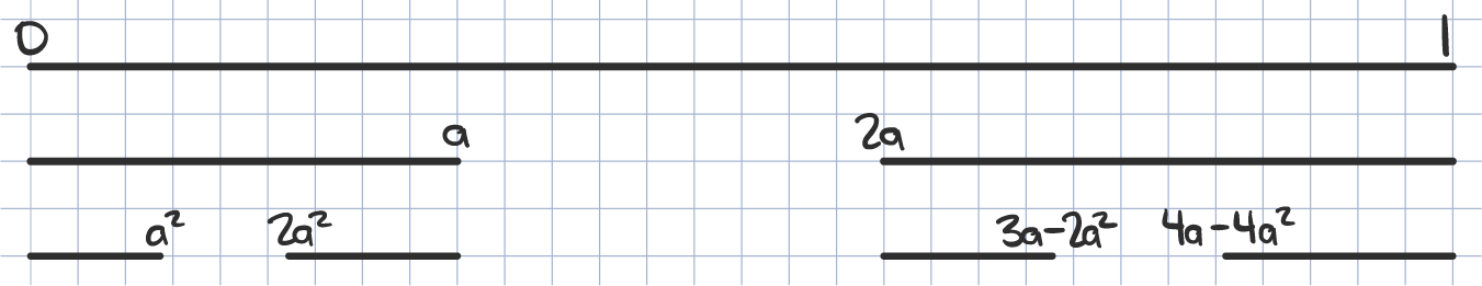


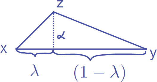


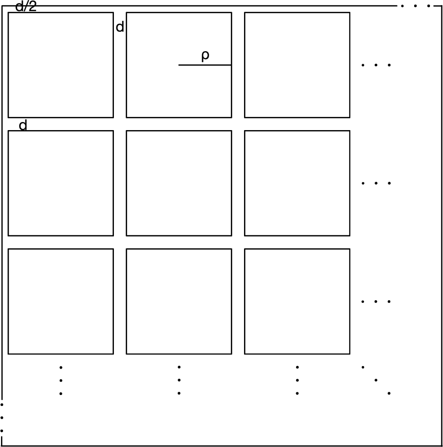


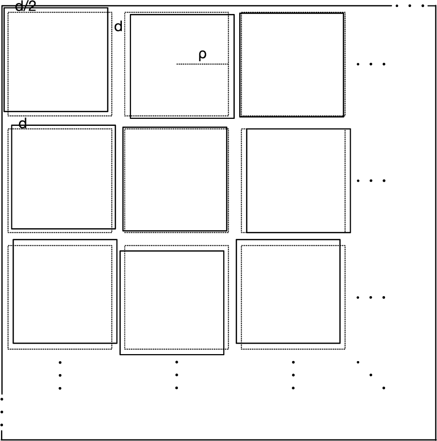


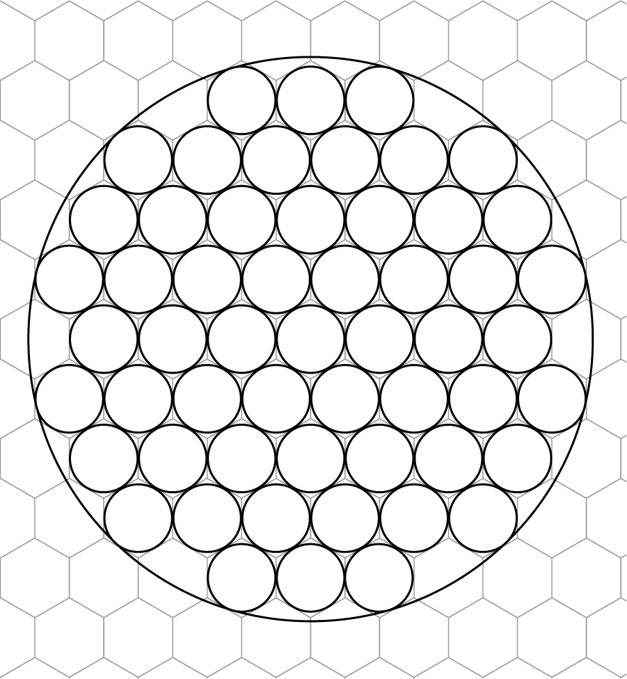


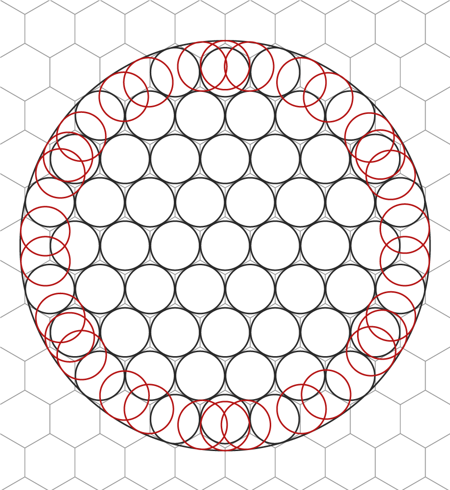


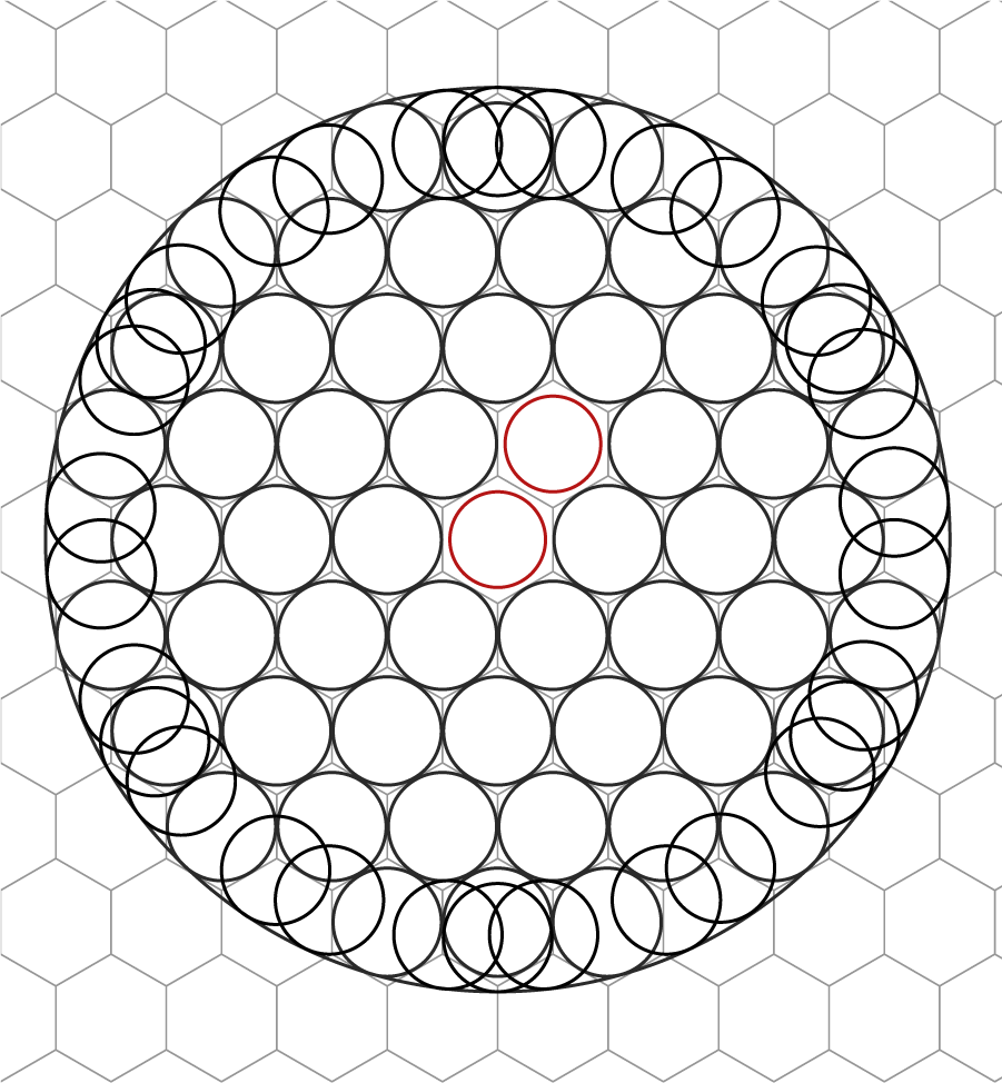


 Open access