




Introduction
Antarctic sea ice regulates climate by reflecting solar radiation and moderating air-sea gas exchange (Massom & Stammerjohn Reference Massom and Stammerjohn2010). On a local scale, the expulsion of salt during ice formation leads to the sinking of dense, highly saline Antarctic Bottom Water (AABW). Associated areas of upwelling bring nutrients to the surface, making the sea-ice zone an optimal habitat for marine life across all trophic levels (Massom & Stammerjohn Reference Massom and Stammerjohn2010). Despite the importance of Antarctic sea ice in the climate system, little is known about how its distribution has changed in response to the Holocene atmospheric temperature fluctuations observed in both coastal (Mulvaney et al. Reference Mulvaney, Triest and Alemany2014) and continental ice-core records (e.g. EPICA Community Members 2006). For example, an ice core from James Ross Island in the north-western Weddell Sea shows stable temperatures from 9200 to 2500 yr bp followed by pronounced cooling from 2500 to 600 yr bp (Mulvaney et al. Reference Mulvaney, Abram, Hindmarsh, Arrowsmith, Fleet and Triest2012). A proximal marine core (Vega Drift) suggests a long-term increase in annual sea-ice duration from 5000 to 1900 yr bp, potentially linked to enhanced sea-ice transport from the southern Weddell Sea (Barbara et al. Reference Barbara, Crosta, Leventer, Schmidt, Etourneau, Domack and Massé2016), as well as ‘unstable’ conditions from 1900 yr bp to present. However, there are few data available on sea ice for the southern and eastern Weddell Sea to understand the relationship between atmospheric temperatures and sea-ice extent. Here, we present a reconstruction of late Holocene sea-ice extent in the south-eastern Weddell Sea from proxies preserved in regurgitated seabird stomach-oil deposits.
Snow petrels (Pagodroma nivea) form colonies on ice-free terrain up to 440 km inland (Francis et al. Reference Francis, Wakefield, Jamieson, Phillips, Hodgson and Southwell2025). Snow petrels eject their proventricular stomach oil at nesting sites as a defence mechanism (Matthews Reference Matthews1949, Warham et al. Reference Warham, Watts and Dainty1976). Over time, the stomach oil builds up with a layered stratigraphy (Fig. 1c), providing a long-term record of their diet and indirect evidence of the sea-ice and open water habitats within their foraging range (e.g. McClymont et al. Reference McClymont, Bentley, Hodgson, Spencer-Jones, Wardley and West2022). Snow petrels will typically forage for fish, Antarctic krill and squid, which can be distinguished using biochemical signatures in their stomach-oil deposits (Ainley et al. Reference Ainley, Hobson, Crosta, Rau, Wassenaar and Augustinus2006, Berg et al. Reference Berg, Melles, Hermichen, McClymont, Bentley, Hodgson and Kuhn2019, Reference Berg, Emmerson, Heim, Buchta, Fromm and Glaser2023, McClymont et al. Reference McClymont, Bentley, Hodgson, Spencer-Jones, Wardley and West2022). Previous observations (Ainley et al. Reference Ainley, O’Connor and Boekelheide1984, Delord et al. Reference Delord, Kato, Tarroux, Orgeret, Cotté and Ropert-Coudert2020) suggest that snow petrels foraging at or within the sea-ice margin and coastal habitats are likely to consume a diet higher in fish (Hodum & Hobson Reference Hodum and Hobson2000, La Mesa et al. Reference La Mesa, Eastman and Vacchi2004), whereas snow petrels foraging in pelagic waters, beyond the continental shelf, are likely to consume a diet higher in Antarctic krill (Obst Reference Obst1985, Ainley et al. Reference Ainley, Hobson, Crosta, Rau, Wassenaar and Augustinus2006). Within high sea-ice concentrations (> 80%), strong winds at the ice-sheet margin or offshore upwelling zones can give rise to areas of open water described as ‘coastal’ or ‘sensible-heat’ polynyas, respectively (Stroeve et al. Reference Stroeve, Jenouvrier, Campbell, Barbraud and Delord2016), which also offer snow petrel foraging habitats (Ainley et al. Reference Ainley, O’Connor and Boekelheide1984). Modern snow petrel tracking shows foraging occurring between ~500 and > 1500 km from nests, with shorter distances (< 500 km) during the brood-guard phase, moderate distances (~500–1000 km) during egg incubation and much greater distances (> 1000 km) during the pre-laying and pre-breeding season (Wakefield et al. Reference Wakefield, McClymont, Descamps, Grecian, Hoelzel and Honan2025). However, snow petrels will not sustain a breeding colony if the sea-ice edge remains beyond their foraging range unless polynyas are present within the pack ice (e.g. Barbraud et al. Reference Barbraud, Weimerskirch, Guinet and Jouventin2000, Thor & Low Reference Thor and Low2011, Viola et al. Reference Viola, Wienecke, Green, Corney, Raymond and Southwell2023).
a. Overview map of the regional study area using data from the Scientific Committee on Antarctic Research (SCAR) Antarctic Digital Database 2023 (https://data.bas.ac.uk/items/e74543c0-4c4e-4b41-aa33-5bb2f67df389/), with main bathymetric and glaciological features surrounding 1401MUM1 (yellow circle) and snow petrel foraging ranges from 700 to 1000 km (dashed semicircles; Wakefield et al. Reference Wakefield, McClymont, Descamps, Grecian, Hoelzel and Honan2025). The Filchner-Ronne Ice Shelf and Berkner Island are labelled, as well as the nearby ice shelves. Present snow petrel colonies are shown (white circles; Francis et al. Reference Francis, Wakefield, Jamieson, Phillips, Hodgson and Southwell2025), as are local ice core records (ITASE IceReader: http://www.icereader.org/icereader/listData.jsp; Climate Change Institute Antarctic Ice Core Data: http://cci.icecoredata.org/Antarctica.html; WAIS Divide Project summary paper: https://www.nature.com/articles/nature12376) and grounded ice extents from 20 to 5 ka (Bentley et al. Reference Bentley, Cofaigh, Anderson, Conway, Davies and Graham2014). Summer sea-ice extent from the last 2 ka (Thomas et al. Reference Thomas, Allen, Etourneau, King, Severi and Winton2019) and median summer sea-ice extent (1981–2010; Crosta et al. Reference Crosta, Kohfeld, Bostock, Chadwick, Du Vivier and Esper2022) are shown. The inset map shows the study area within the context of the wider continent of Antarctica, and the dashed box shows the satellite image location of E. b. Map of the Theron Mountains with deposits shown at Marø and Coalseam cliffs. c. Photograph of 1401MUM1 after cutting in half showing millimetre-scale laminations, before analysis. d. Photograph of the Marø cliff face, where snow petrels will typically nest in rock crevices (photo credit: M. Bentley and D. Hodgson, 2015). e. Modern-day Moderate Resolution Imaging Spectroradiometer (MODIS) satellite imagery acquired December 2002 from the Terra satellite, showing the seasonal summer sea ice in the Weddell Sea and the presence of a band of thinner sea ice and coastal polynyas along the front of the Filchner-Ronne Ice Shelf (J. Descloitres, MODIS Rapid Response Team and NASA/GSFC: Weddell Sea image from Terra satellite, data acquired 12 December 2002, published 30 December 2002).

We use radiocarbon dating, lipid biomarkers (FAs, sterols and n-alkanols), stable isotopes and elemental information to decipher the past summer sea-ice foraging habitats of a snow petrel colony in the Theron Mountains, whose foraging range spans the eastern Weddell Sea (Fig. 1a). From this analysis, we reconstruct a high-resolution late Holocene record of changes in snow petrel diet to infer past changes in sea-ice extent and characteristics within their foraging range. We then compare these with marine sediment and ice-core proxy records to gain a better understanding of the relationship between climate and sea ice. Given the widespread distribution of snow petrel stomach-oil deposits in East Antarctica (e.g. Ainley et al. Reference Ainley, Hobson, Crosta, Rau, Wassenaar and Augustinus2006, Berg et al. Reference Berg, Melles, Hermichen, McClymont, Bentley, Hodgson and Kuhn2019, McClymont et al. Reference McClymont, Bentley, Hodgson, Spencer-Jones, Wardley and West2022, Stevenson et al. Reference Stevenson, Hodgson, Bentley, Gröcke and McClymont2025), there is potential for the methods applied here, alongside future recovery of new samples, to provide detailed reconstructions of changes to Antarctic sea-ice environments in regions where data are currently scarce.
Materials and methods
Regional context
Stomach-oil deposits were sampled at Marø Cliffs (79.039°S, 28.262°W) in the Theron Mountains (Fig. 1), situated ~250 km from the coast. Thermal-infrared satellite imagery from December 2002 (Fig. 1e) shows high frequencies of thin ice in the southern and eastern Weddell Sea, including areas of open water or polynyas within the sea ice and along the edge of the Filchner-Ronne Ice Shelf. Polynyas are formed where there is wind-driven Ekman transport and upwelling of warm, nutrient-rich water and at the ice front due to localized katabatic winds. Modern observations show coastal polynya(s) as large as 3516 ± 1420 km2 in the south-eastern Weddell Sea (Paul et al. Reference Paul, Willmes and Heinemann2015). Alternative foraging areas include ‘post-polynyas’ - locations where polynyas opened within the winter sea-ice pack and enabled early or high seasonal primary productivity (Arrigo et al. Reference Arrigo, van Dijken and Strong2015) - which remain biological hotspots attractive to seabirds year round (Brierley & Thomas Reference Brierley and Thomas2002). Polynyas at the ice-shelf front can also experience high productivity enhanced by iron from nearby coastal glacier melt (Arrigo et al. Reference Arrigo, van Dijken and Strong2015).
Stomach-oil deposits
We focused on deposit 1401MUM1 (79.049°S, 28.329°W; Fig. 1c), which had excellent preservation of internal millimetre-scale layering consisting of sub-parallel orange, yellow and brown laminations. One half of the deposit was preserved for non-destructive core scanning and archiving, and the other half was sub-sampled for geochemical analysis. Visual colour analysis was based on the Munsell colour system (Briggs et al. Reference Briggs2023).
Radiocarbon ( 14 C) analysis
A chronology was established from eight radiocarbon dates from the top and bottom of the deposit and at visually distinct layers or geochemical variations. Samples were digested in 1 M HCl (80°C, 2 h), washed free of mineral acid with deionized water, dried and homogenized. The total carbon in a known weight of the pre-treated sample was recovered as CO2 by heating with CuO in a sealed quartz tube. The gas was converted to graphite by Fe/Zn reduction. The results are reported as conventional radiocarbon years bp (relative to ad 1950) and % modern 14C to ± 1σ level, corrected to δ13C = −25‰ using a δ13C value obtained by measurement of a CO2 aliquot of the sample. The δ13C value was measured on a Thermo Fisher Delta V stable isotope mass spectrometer and represents the δ13C value of the pre-treated sample.
MARINE20 radiocarbon age calibration (Heaton et al. Reference Heaton, Köhler, Butzin, Bard, Reimer and Austin2020) was carried out using CALIB 14C (Stuiver & Reimer Reference Stuiver and Reimer1993). To account for the Southern Ocean marine reservoir effect, a ΔR of 670 ± 50 years was applied, derived from pre-bomb 14C ages at Hope Bay in the north-western Weddell Sea (Björck et al. Reference Björck, Hjort, Ingolfsson and Skog1991). This ΔR reflects a ‘no sea ice’ scenario as defined by Heaton et al. (Reference Heaton, Köhler, Butzin, Bard, Reimer and Austin2020), which is applicable to the late Holocene. The BACON (v2.3.9.1) package in R 3.6.0 (Blaauw & Christen Reference Blaauw and Christen2011) was used to generate an age-depth model.
Elemental analysis
Non-destructive elemental analysis was conducted by qualitative X-ray fluorescence (XRF) on a GeoTek core scanner (MSCL-XYZ) measuring at 1 mm intervals downcore using a rhodium source X-ray generator at 10 mm cross-core slit width. Counting time was 10 s for each of the four beams (Beam 1: no filter, 10 kV generator voltage; Beam 2: 25 μm silver filter, 20 kV generator voltage; Beam 3: 125 μm silver filter, 30 kV generator voltage; Beam 4: 625 μm copper filter, 50 kV generator voltage). The energies of the photons detected were between ~2 and 35 keV.
The data were first screened using the tidyverse package in R 3.6.0 (Wickham et al. Reference Wickham, Averick, Bryan, Chang, McGowan and François2019). Samples with poor data quality, system artefacts (e.g. Ag, Au, Rh) or missing or negative values were removed. Where elements appeared in more than one beam, the first beam was used. Cluster analysis was carried out using the rioja package (Juggins Reference Juggins2023), with a broken-stick model used to identify statistically significant clusters with similar geochemical characteristics (Bennett Reference Bennett1996). Principal component analysis (PCA) was performed in PAST3 (Hammer et al. Reference Hammer, Harper and Ryan2001) to identify the key relationships between the elemental, stable isotope, biomarker and total organic carbon (TOC) data.
Bulk stable isotope analysis
Contiguous subsamples were taken by 2 mm biopsy punch at 3 mm spacing. Stable isotopes were measured on a Costech elemental analyser (ECS 4010) connected to a Thermo Scientific Delta V Advantage isotope ratio mass spectrometer. Carbon isotope ratios (δ13C) were corrected for 17O and reported in standard delta (δ) notation in per mil (‰) relative to Vienna PeeDee Belemnite (VPDB). Nitrogen isotope ratios (δ15N) are reported against atmospheric nitrogen (AIR). Isotopic accuracy was monitored through multiple daily analysis of international (e.g. IAEA-600, IAEA-CH-3, IAEA-CH-6, IAEA-N-1, IAEA-N-2, NBS 19, USGS24, USGS40) and in-house standards. These standards provided a linear range for δ13C between −46‰ and +3‰ and for δ15N between −4.5‰ and +20.4‰. Analytical uncertainty was typically ± 0.1‰ (2 SD) for replicate analyses of the international standards and < 0.2‰ (2 SD) on replicate sample analysis. TOC and nitrogen data were obtained as part of the isotopic analysis using the internal standard, glutamic acid (40.82 wt% C, 9.52 wt% N).
Biomarker analysis
Biomarker subsamples were taken adjacent to the stable isotope subsamples. Lipid biomarkers were extracted from 0.05–0.9 g of sample using repeated ultra-sonication (3 × 15 min) with 4 ml of dichloromethane (DCM):methanol (MeOH) at a ratio of 3:1. Four internal standards were added (5α-androstan-3β-ol (0.02 g), 5α-androstane (0.02 g), 2-nonadecanone (0.08 g) and heptadecanoic acid (0.14 g of C17:0)) to each sample. After each sonication, samples were centrifuged for 2 min at 2000 rpm. The total lipid extract (TLE) was combined in round-bottom flasks and taken to dryness using a rotary evaporator. Between 20 and 45 mg of TLE were recovered from this process.
Once extracted, 1 ml KOH:MeOH (8% KOH) was added to the TLE, placed on a hotplate for 1 h at 70°C and left overnight to cool. Repeated rinses with 3 ml hexane extracted the neutral lipid fraction (e.g. alkanols and sterols). The remaining solution was acidified using hydrochloric acid (HCl), and FAs were recovered using repeated rinses of hexane. FAs were methylated to FA methyl esters (FAMEs) by adding 3 ml of 95:5 MeOH:HCl to each test tube, which were then foiled, capped and heated at 70°C for 12 h, then allowed to cool to room temperature. Finally, 4 ml of DCM-cleaned water was added and rinsed with repeated additions of 3 ml hexane:DCM (4:1). FAME fractions were then taken to dryness in a stream of N2.
FAMEs were diluted in 500 μl of hexane and injected into the gas chromatograph fitted with a flame ionization detector (GC-FID) or mass spectrometer (GC-MS). Samples were first screened by GC-FID using a RXi-5MS 60 m column with conditions as follows: 1 μl sample injection volume; splitless injection; injection temperature 280°C; split flow 50 ml/min; flow rate 2.3 ml/min, with oven temperature at 45°C hold for 1.2 min; ramp at 10°C/min to 160°C; ramp at 4°C/min to 310°C; hold at 310°C for 25 mins. Analysis by GC-MS used a 30 m FAMEWAX column with conditions as follows: 0.8 μl sample injection volume; programmable temperature vaporizing injection (PTV) splitless mode; injection temperature 230°C; split flow 15 ml/min; flow rate 1.5 ml/min, with oven temperature at 100°C hold for 3 min; ramp at 2°C/min to 230°C hold for 10 min. The MS settings were electron ionization (EI) mode; helium carrier gas; MS transfer line 230°C; ion source temperature 230°C; scan mode: mass range 38–600 (amu). Compound identification was performed using the National Institute of Standards and Technology (NIST) reference library. Biomarkers were quantified through reference to the internal standard using the total ion current (TIC) from the GC-MS.
To isolate fatty alcohols (FAlcs) and sterols, the neutral fraction was fractionated using flash column chromatography. A glass pipette was packed with 4 cm deactivated silica (heated 140°C for 16 h, with a silica pore size of 60 Å, 220–240 mesh particle size, 35–75 μm particle size; Sigma-Aldrich 60738-1KG). After column conditioning with hexane (×3 column volumes), the sample was added in 500 μl DCM. Elution occurred in the following order: hexane (Fraction 1, apolar compounds), DCM (Fraction 2, ketones), DCM:methanol (1:1; Fraction 3, polar compounds). All fractions were decanted and transferred into GC vials and evaporated to dryness in a stream of N2. Fraction 3 was then further derivatized to trimethylsilyl esters prior to analysis using 50 μl DCM and 50 μl BSTFA (N,O-Bis(trimethylsilyl)trifluoroacetamide) with 1% TMCS (chlorotrimethylsilane) heated for 1 h at 70°C and left overnight. Samples were evaporated to dryness and dissolved in hexane prior to analysis. GC-MS analysis used a Restek RXi-5MS (crossbond 5% diphenyl/95% dimethyl polysiloxane) column (60 m × 0.25 mm × 0.25 um) at 0.8 μl sample injection volume; PTV splitless mode; injection temperature at 280°C; split flow 23 ml/min; flow rate 2.3 ml/min, with oven temperature at 50°C hold for 2 min; ramp at 10°C/min to 200°C and then ramp at 3°C/min to 300°C and hold for 20 min. The MS settings were EI mode with helium carrier gas, MS transfer line 310°C and ion source temperature 300°C. The scan mode was set at mass range 50–550 (amu).
Rock analysis
To determine local bedrock chemistry, a sample of bedrock attached to 1401MUM1 was soaked in ethanol to remove stomach-oil residue (repeated three to four times). The sample was then crushed using a fly press, freeze dried for 48 h and ground to a fine, homogeneous powder using a ball mill. Organic matter was removed by adding 4 ml of 30% hydrogen peroxide to a ~0.5 g aliquot of rock. The sample was then digested for 4 h in 16 ml of Aqua Regia using a DigiPREP digestion block and subsequently diluted to 50 ml with deionized water and filtered at 0.45 μm. Elemental composition was determined using an Agilent Technologies 5100 inductively coupled plasma optical emission spectrometer (ICP-OES).
Results
Stratigraphy
1401MUM1 is laminated, with four different colour changes (Fig. 1c). The base (120–90 mm depth) is dark brown (Munsell hex code #342617ff), 90–45 mm is light yellow (Munsell hex code #5d4125ff) and 45–20 mm is dark brown/orange (Munsell hex code #3d260fff). The surface 20–0 mm is light yellow (Munsell hex code #947c58ff), possibly as a result of prolonged subaerial exposure. Sub-parallel laminations suggest stratigraphic accumulation of oils without major reworking of material. Some inclined unit boundaries and laminations observed closer to the nesting site (right side in Fig. 1c) suggest accumulation behind an obstacle (e.g. a rock). The XRF scan was conducted down the deposit centre to ensure parallel laminations were captured. Smaller black inclusions were also present (Fig. 1c), which we attribute to guano.
Radiocarbon analyses show a median calibrated (cal.) age of 1734 ± 210 cal. yr bp at the base of the deposit, 831 ± 178 cal. yr bp at the surface and no age reversals (Table I). The age-depth model is relatively linear (Fig. S1). The accumulation rate varies between ~9 and 18 mm/century.
Radiocarbon ages and calibrated calendar ages for deposit 1401MUM1. Ages were calibrated in BACON (v2.3.9.1; Blaauw & Christen Reference Blaauw and Christen2011) using the MARINE20 calibration (Heaton et al. Reference Heaton, Köhler, Butzin, Bard, Reimer and Austin2020) and the nearest Holocene ΔR of 670 ± 50 years (Björck et al. Reference Björck, Hjort, Ingolfsson and Skog1991).

XRF = X-ray fluorescence.
Elemental composition
Cluster analysis identified three significant units - Unit III (oldest) to Unit I (youngest) - broadly corresponding to the colour changes (Fig. 2a). Unit III (120–90 mm) is characterized by near-mean values (grey lines in Fig. 2) of Al, Si and Ti, below-mean values for Te, Br and Ni and above-mean values for Cu. Unit II (90–20 mm) is characterized by initially below-mean values for Al, Cu, Si and Ti, increasing throughout the unit to above-mean values. Te, Br and Ni are initially above-mean values but sharply decrease in the upper part of Unit II. Unit I (20–0 mm) is characterized by near-mean values of Al, Si, Te and Ti, below-mean values for Cu and above-mean values for Br and Ni. PCA analysis (Fig. 2b) shows Al, Fe, Si and Ti grouping together with strong negative loading on PC1 at depths corresponding to Units I and III. Br and Ni have a strong positive loading broadly corresponding to Unit II. PC1 accounts for just under 29% of the variance. Cu, Sn and Te have a positive loading along PC2, which accounts for 17% of the variance. The elemental composition of the bedrock clast incorporated into the deposit is dominated by Si, Ti, Ca and Al (Fig. 3).
a. Key elemental and trace metal X-ray fluorescence (XRF) results downcore for 1401MUM1. White stars indicate where radiocarbon dates were taken, with original data points at 1 mm spacing shown by the grey solid lines and 10 mm moving averages shown by the coloured lines. Vertical grey dashed lines indicate mean values, with Al = 150 counts per second (cps), Fe = 4000 cps, Ti = 500 cps, Cu = 85 cps, Te = 15 cps, Br = 200 cps and Ni = 40 cps. Cluster boundaries are determined by constrained hierarchical clustering analysis in the rioja package of R (Juggins 2020) compared to a broken-stick analysis (Bennett Reference Bennett1996). Three significant clusters (Units I–III) were identified based on the XRF data, with Unit II marked by horizontal shading. b. Principal component analysis (PCA) of the XRF data to identify key elemental relationships and different origins, shaded by sample depth. c. PCA of fatty acids, total organic carbon (TOC), Ti and stable isotope data, noting the contribution of fatty acids (positive loading along PC2) and degradation (negative loading along PC2). All PCAs were generated using PAST3 (Hammer et al. Reference Hammer, Harper and Ryan2001).

Accumulation rate, key fatty acid (FA) ratios, bulk δ13C and δ15N, total organic carbon (TOC), potential degradation proxies and PC2 (FA) for 1401MUM1 downcore. White stars indicate where dates were taken and grey dashed lines mark mean values. Cluster boundaries are determined by constrained hierarchical clustering analysis of the X-ray fluorescence (XRF) data in the rioja package of R (Juggins 2020) compared to a broken-stick analysis (Bennett Reference Bennett1996). Three significant clusters (Units I–III) were identified based on the XRF data, with Unit II marked by horizontal shading. PC2 is plotted to show peaks in the organic contribution (positive values) relative to degradation signals (negative values).

FA ratios, bulk stable isotopes and TOC
PCA analysis of FAs, bulk stable isotopes and TOC shows that PC1 accounts for 56% of the variance, with the positive loading largely driven by FAs and the negative loading by TOC, with a smaller influence of δ13C (Fig. 2c). PC2 is largely driven by differences in FA composition (~21% of the variance). A group of saturated and monounsaturated FAs (C14:0, C15:0, C16:0, C18:0, C18:1 and C18:2) have a positive loading at depths corresponding to Units III and II. The remaining FAs (C9:0, C13:0 and C16:1) have a strong negative loading at depths corresponding to Unit I. The relative contributions of C18:1 compared to the main saturated FAs (expressed as C18:1:C14:0, C18:1/(C18:1 + C16:0) and C18:1:C18:0) downcore (Fig. 3) have above-mean values in Unit III, decreasing to below-mean values in Unit II and near-mean values in Unit I. The contribution of C14:0 relative to C16:0, expressed as C14:0/(C14:0 + C16:0), is characterized as near-mean values in Units III, II and I, with a few deviations towards the top of Unit II.
δ13C and δ15N have broadly similar trends (Fig. 3). δ13C is characterized by above-mean (−29‰) values in Unit III, decreasing to below-mean values towards the top of Unit II and near-mean values in Unit I. δ15N is characterized by above-mean values in Unit III (14‰), decreasing to below-mean values from near the base of Unit II and continuing into Unit I. δ13C and δ15N have a positive loading on PC2 (Fig. 3c). TOC (Fig. 3) is characterized by below-mean percentages in Unit III and above-mean percentages in Units II and I. Expressed as a flux, TOC is low in Unit III, increases to its highest values at the base of Unit II, then declines through the rest of Unit II and into Unit I (Fig. 3).
Discussion
We first interpret the stomach-oil accumulation rate in relation to changes in snow petrel occupation history, then draw on both elemental and organic data to infer changes in snow petrel diet. Drawing on these interpretations, we infer sea-ice changes in the Weddell Sea during the late Holocene and explore links with regional palaeoclimate records.
Proxy interpretations drawing on fatty acid and X-ray fluorescence analysis.

Accumulation rate and occupation history
The stomach-oil accumulation rate is a proxy for changes in snow petrel nest occupation. Where snow petrels have good access to foraging grounds, more frequent and sustained nest occupation is expected, which would in turn lead to higher accumulation rates of stomach oils. However, the total accumulation rate might also be affected by minerogenic inputs (e.g. from locally eroded clasts or wind-blown dust; Li et al. Reference Li, Ginoux and Ramaswamy2008, Duprat et al. Reference Duprat, Kanna, Janssens, Roukaerts, Deman and Townsend2019). In Unit III, high inputs of Al, Fe and Si, which are also found in local bedrock (Fig. S3) and are attributed to minerogenic sources in other deposits (Berg et al. Reference Berg, Melles, Hermichen, McClymont, Bentley, Hodgson and Kuhn2019, McClymont et al. Reference McClymont, Bentley, Hodgson, Spencer-Jones, Wardley and West2022), suggest that the elevated accumulation rate here may be the result of higher inputs of bedrock and wind-blown inputs rather than high stomach-oil accumulation.
In contrast, the declining accumulation rate in upper Unit II into Unit I (Fig. 3) is marked by an overall decline in TOC, confirming that there was reduced oil accumulation during the late Holocene (Fig. 3). We interpret this pattern as representing a drop in regurgitations and intermittent stomach-oil deposition caused by foraging habitat lying relatively far from the nesting sites, which, in turn, made occupation more challenging.
Sea-ice signals in elemental data
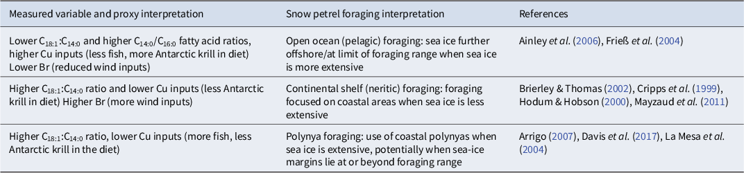
The elements Cu and Sn group separately to the minerogenic elements discussed earlier (Al, Si, Ti). As Cu is involved in the transport of oxygen-carrying hemocyanin in Antarctic krill (Wang & Zhu Reference Wang and Zhu2022), this group is most probably of organic, Antarctic krill-based origin, prominent in Unit III and the top of Unit II. Where the Cu concentration is lower in the top half of Unit II, this is interpreted as being due to both a reduction in the contribution of Antarctic krill species and a reduction in access to the pelagic waters where Antarctic krill tend to be found during the snow petrel breeding season (Table I; Siegel et al. Reference Siegel, Reiss, Dietrich, Haraldsson and Rohardt2013, Corsolini & Borghesi Reference Corsolini and Borghesi2017).
Br and Ni group separately to the organic or minerogenic groups (Fig. 2b). Although both elements are present in phytoplankton (e.g. John et al. Reference John, Liang, Pasquier, Holzer and Silva2024) and so might reflect direct inputs from stomach oils, Ni was not recorded as an element that is transported to breeding colonies by Antarctic seabirds and was argued to have a minerogenic source (Castro et al. Reference Castro, Neves, Francelino, Schaefer and Oliveira2021). As Ni was a minor contributor to the Theron Mountains bedrock (Fig. S3) and plots separately on the PCA from minerogenic inputs, atmospheric transport of dust could account for the presence of Ni within the deposit. Wind transport may also explain the Br signal (Table II). Bromide ions (Br-) from seawater become concentrated in sea ice as it forms, which can be released into the atmosphere as reactive bromine gases from ice or sea spray (Hara et al. Reference Hara, Osada, Yabuki, Takashima, Theys and Yamanouchi2018). Bromine compounds can also be transported over long distances by winds, particularly during the Antarctic spring when bromine explosion events are most active, suggesting bromine can be used as a wind proxy (Frieß et al. Reference Frieß, Hollwedel, König-Langlo, Wagner and Platt2004). In the lower half of Unit II, where bromine is above average but Cu and minerogenic element values are low, we suggest that the elevated Br reflects increased localized winds and a more extensive sea-ice pack (Table II). As the accumulation rate is high but Cu is low, we propose that the snow petrels had good access to foraging habitats, but that these were low in Antarctic krill. We suggest that this scenario could be explained by enhanced opening of sea ice under more intense wind action, close to the coast (i.e. as coastal polynyas; Table II). Where Br drops to below-mean values (Unit II, upper half), we suggest that reduced winds limited openings in the sea ice, so driving snow petrels further (> 1000 km) to the sea-ice edge and the pelagic, Antarctic krill-rich waters suggested by elevated Cu. During this extensive sea-ice scenario, the decrease in accumulation rate suggests that the Theron Mountains lay close to the limit of the foraging range, allowing wind-blown dust or bedrock to become entrained within 1401MUM1.
Linking biochemistry to snow petrel diet
We observe shifts in bulk stable isotopes, TOC and lipid biochemistry in 1401MUM1. To assess the interpretation of these trends in terms of diet and sea-ice environments, in this section we outline the links between modern biochemistry and the signals recorded in stomach-oil deposits (summarized in Table II).
Synthesis of key X-ray fluorescence, fatty acid (FA) and stable isotope results alongside regional palaeoclimate proxies. Units III–I marked by vertical dotted black lines. a. Fe (counts per second; cps) of 1401MUM1. b. Cu (cps) of 1401MUM1. c. C18:1/(C18:1 + C16:0) FA ratio. d. δ15N of 1401MUM1. e. δ13C of 1401MUM1. f. Record of sea-salt sodium (ssNa) flux from the EPICA Dronning Maud Land (EDML) ice core (75.0025 8°S, 0.0684 8°E; Fischer et al. Reference Fischer, Fundel, Ruth, Twarloh, Wegner and Udisti2007), implying winter sea ice (WSI). g. Diatom assemblages from Piston core JPC38, north-east (NE) Antarctic Peninsula, (63.717°S, 57.411°W), grouped according to their ecological affinities: cold/open water; wind/storminess and sea ice (Barbara et al. Reference Barbara, Crosta, Leventer, Schmidt, Etourneau, Domack and Massé2016). h. Ratio of highly branched isoprenoids (HBIs), [HBI:2]/[HBI:3], from Piston core JPC38, reflecting the relative contribution of sea-ice algae [HBI:2] vs open-water phytoplankton [HBI:3] to the sediment (Barbara et al. Reference Barbara, Crosta, Leventer, Schmidt, Etourneau, Domack and Massé2016). i. DML07 ice core xsSO42- flux (−75.58°S, 3.43°E; Thomas et al. Reference Thomas, Vladimirova, Tetzner, Emanuelsson, Chellman and Dixon2023). j. δ18O values of the EDML ice core, corrected for sea-level change to indicate changes in ocean water temperatures (EPICA Community Members 2006). k. Atmospheric CO2 record from Dronning Maud Land (Siegenthaler et al. Reference Siegenthaler, Monnin, Kawamura, Spahni, Schwander, Stauffer and Fischer2005). l. Hyperspectral ratio (R850/R900), a ratio of reflectance between 850 and 900 nm from a lake sediment record located on the sub-Antarctic Macquarie Island (54°S, 158°E), interpreted as changes in the strength of Southern Hemisphere (SH) westerlies (Saunders et al. Reference Saunders, Roberts, Perren, Butz, Sime and Davies2018). m. Accumulation (accum.) rate of 1401MUM1. SIC = sea-ice concentration.

The biochemistry of snow petrel stomach oil, derived from prey remains, is dominated by saturated FAs such as myristic acid (C14:0), palmitic acid (C16:0) and stearic acid (C18:0), which contribute to the energy content of the oil (Connan et al. Reference Connan, Cherel and Mayzaud2007, Berg et al. Reference Berg, Emmerson, Heim, Buchta, Fromm and Glaser2023). Monounsaturated FAs (C16:1, C18:1, C18:2) in stomach-oil deposits are typically lower in concentration than the original oils due to post-depositional degradation but are still a significant contribution (Berg et al. Reference Berg, Emmerson, Heim, Buchta, Fromm and Glaser2023). FAlcs, derived from the reduction of the carboxyl group in FAs, are also present in 1401MUM1 in both saturated and unsaturated forms (Fig. S2). Cholesterol, a vital element of animal cell membranes and in high abundance in copepods (Havlíčková et al. 2023), is present in 1401MUM1 in low concentrations (Fig. S2). The varying proportions of these compounds are indicative of changing contributions of marine prey to the snow petrel diet.
Major marine prey species for snow petrels include Antarctic krill (Euphausia superba), Antarctic lanternfish (Electronica antarctica), Antarctic silverfish (Pleuragramma antarcticum) and squid, with small contributions of ice krill (Euphausia crystallorophias; Ainley et al. Reference Ainley, O’Connor and Boekelheide1984, Ferretti et al. Reference Ferretti, Soave, Casaux and Coria2001, Fijn et al. Reference Fijn, Van Franeker and Trathan2012, Rodhouse Reference Rodhouse2013, Viola et al. Reference Viola, Wienecke, Green, Corney, Raymond and Southwell2023). Elevated concentrations of C16:0 compared to other saturated FAs could indicate increased squid uptake (Cripps et al. Reference Cripps, Watkins, Hill and Atkinson1999, Corsolini & Borghesi Reference Corsolini and Borghesi2017), whereas an increasing C18:1 concentration relative to C14:0 and C16:0 could indicate an increased uptake of fish (E. antarctica and P. antarcticum; Mayzaud et al. Reference Mayzaud, Chevallier, Tavernier, Moteki and Koubbi2011) relative to Antarctic krill (Table II; Cripps et al. Reference Cripps, Watkins, Hill and Atkinson1999).
Once regurgitated, lipid biomarkers may undergo post-depositional alteration, affecting their preservation signals as the oil accumulates. The oxidation of unsaturated FAs, decarboxylation and β-oxidation can modify these compounds, producing oxidative products and FAlcs (Warham et al. Reference Warham, Watts and Dainty1976). The chemical instability of the monounsaturated FAs C16:1 and C18:1 and the di-unsaturated FA C18:2 due to preferential oxidation can lead to lower concentrations that are not reflective of the original dietary contributions (Gyamfi et al. Reference Gyamfi, Ofori Awuah, Owusu and Patel2019). This process can be facilitated microbially, leading to elevated C13:0 and C15:0 concentrations (Volkman et al. Reference Volkman, Barrett, Blackburn, Mansour, Sikes and Gelin1998). Previous dietary studies of Southern Ocean seabirds (Connan et al. Reference Connan, Cherel and Mayzaud2007, Berg et al. Reference Berg, Emmerson, Heim, Buchta, Fromm and Glaser2023) have, however, identified low monounsaturated FA concentrations to be consistent with dietary shifts, so we consider both sources during our analysis.
Large shifts in bulk δ15N are observed in 1401MUM1, which range between 10‰ and 14‰ (0–65 mm) or > 14‰ (> 65 mm). Higher bulk δ15N values, typically by 2–3‰, can reflect a shift in foraging habitat towards lower latitudes (Rau et al. Reference Rau, Ainley, Bengston, Torres and Hopkins1992) or a trophic level shift (e.g. from Antarctic krill to fish; Cherel et al. Reference Cherel, Hobson, Guinet and Vanpe2007). In 1401MUM1, trophic shifts probably influenced the nitrogen isotope signal given the grouping of δ15N alongside dietary FAs (Fig. 2c). However, we recognize that additions of N-containing materials to the deposits may introduce mixed non-dietary/dietary signals. Snow petrels excrete nitrogenous waste, primarily in the form of uric acid, as a means of eliminating excess nitrogen from their bodies (Shatova et al. Reference Shatova, Wing, Gault-Ringold, Wing and Hoffmann2016, Wu et al. Reference Wu, Sheng, Liu, Zheng, Emslie and Yang2023). Therefore, as guano accumulates, both the %N and bulk δ15N increase (Nie et al. Reference Nie, Liu, Wen, Sun and Emslie2014), which will reduce the C/N ratio (Figs S2 & S5). However, we did not identify any relationship between bulk δ15N and C/N in Unit III or at the beginning of Unit II, so we discount guano as the cause of the elevated δ15N in both units (Figs S2 & S5; Liu et al. Reference Liu, Nie, Sun and Emslie2013, Wang et al. Reference Wang, Liu, Fang, Jin, Wu and Fu2020). An alternative source for N comes from local shale-rich bedrock, with values ranging from 5‰ to 15‰ (Holloway & Dahlgren Reference Holloway and Dahlgren2002). However, similarly high δ15N values (~18‰) have also been recorded in nearby fossilized stomach-oil deposits in the Heimefrontfjella range but where the local bedrock is granitic (Stevenson et al. Reference Stevenson, Hodgson, Bentley, Gröcke and McClymont2025). Comparable or higher values of δ15N have been observed in other Antarctic ornithogenic soils (e.g. Nie et al. Reference Nie, Liu, Wen, Sun and Emslie2014) where inputs are primarily from guano rather than oils. At 1401MUM1, as the shift in δ15N values between Units III and II is too large to be caused by a trophic shift and seems not to have been influenced by bedrock or guano contributions, further work is required to understand the controls on δ15N during the late Holocene period.
A predominantly mixed dietary signature is observed from the FAs at 1401MUM1, although changes to the relative contributions of Antarctic krill, fish and squid prey can be inferred downcore. A fish-dominant signature, as seen in Unit II (the lower half), is characterized by elevated FA C18:1/C14:0 ratios and C18:1/(C18:1 + C16:0) and a drop in Antarctic krill-derived Cu. Higher up in Unit II, elevated C14:0 and reduced C18:1 indicate greater Antarctic krill uptake, supported by a higher Cu content (Fig. 2) and falling δ15N (Fig. 3). This multi-proxy approach has allowed distinct prey shifts to be distinguished from the geochemical record.
Key dietary changes across Units III to I
The low TOC in Unit III (~120–90 mm) and presence of bedrock clasts (Fig. 2) suggest that the high accumulation rate here is driven by elevated minerogenic inputs. Intermittent stomach-oil deposition during this time suggests relatively sporadic nest occupation. The subsequent opportunity for enhanced oxidation or diagenesis of organic material has most probably also resulted in an overall loss of TOC and of monounsaturated FAs with dietary sources (Fig. 3). Of the dietary FAs, the increase in C18:1 relative to C14:0, C16:0 and C18:0 (Fig. 3), alongside above-average Cu (Fig. 2), is consistent with intermittent access to an Antarctic krill- and fish-based diet.
The bottom half of Unit II (~90–50 mm depth) is characterized by below-average Al, Fe, Ti and Cu values, suggesting a reduction in minerogenic and Antarctic krill inputs (Fig. 2). The significant Cu drop just beyond the Unit III–II transition suggests a sudden reduction in Antarctic krill consumption. This coincides with continued relatively elevated contributions of C18:1 (c.f. C18:1/C18:0 and C18:1/(C18:1 + C16:0); Figs 3 & S2) alongside an increase in δ15N (Fig. 3), implying a shift in diet towards E. antarctica and P. antarcticum (Corsolini & Borghesi Reference Corsolini and Borghesi2017). Higher TOC (45%) and low inputs of microbial FA (e.g. C13:0) in Unit II indicate a highly organic unit with low rates of degradation (Berg et al. Reference Berg, Emmerson, Heim, Buchta, Fromm and Glaser2023), driving the high accumulation rate and suggesting a period of high nest occupation.
The top half of Unit II (~50–20 mm depth) is marked by a rapid increase in minerogenic elements, a slow decline in C18:1 ratios (Fig. 3), reduced individual FA concentrations (Fig. S2) and depletion of δ13C. A lower accumulation rate compared to 90–50 mm implies a decline in regurgitations and decreased nest occupation. Although peaks in C13:0 FA and C15:0 FA occur in Unit II, the broadly positive PC2 score suggests that dietary FAs dominate the signal (Fig. 3). The slow decline in the proportion of C18:1 relative to C14:0 (Figs 3 & S2) highlights a longer-term trend of reduced fish in the diet across Units II–I. The rise in Cu above 40 mm (Fig. 2) and drop of δ15N to < 10‰ above 30 mm (Fig. 3) suggest Antarctic krill returning as a dominant prey species.
The onset of Unit I (~20–0 mm) records a decline in Cu compared to Unit II (Fig. 2), suggesting a reduction in the Antarctic krill contribution to the diet. This interpretation is supported by slightly elevated C18:1 FA concentrations (Fig. 3) compared to the tops of Units II and I. Both Cu and TOC (%) show a recovery to levels comparable to the top of Unit II at the very top of Unit I. Unit I is marked by a return to the very low TOC fluxes recorded in Unit III. The contribution of minerogenic elements remains low, suggesting that the reduced organic matter contributions are not due to additions of erosional material. The C13:0 FA peaks (Fig. 3) suggest that microbial activity might have impacted the top of the deposit since the abandonment of the nest through decomposition by bacteria and fungi via aerobic respiration and fermentation (Park et al. Reference Park, Ledesma-Amaro and Nicaud2020). As oil was still accumulating at the site, we suggest that Unit I represents a period of reduced nest occupancy.
Sea-ice variability in the southern Weddell Sea
We have determined that even during the late Holocene variations in snow petrel diet and occupation history occurred. Drawing on the modern associations of snow petrels with sea ice (e.g. Ainley et al. Reference Ainley, O’Connor and Boekelheide1984, Delord et al. Reference Delord, Kato, Tarroux, Orgeret, Cotté and Ropert-Coudert2020, Francis et al. Reference Francis, Wakefield, Jamieson, Phillips, Hodgson and Southwell2025, Honan et al. Reference Honan, Wakefield, Phillips, Grecian, Prince and Robert2025), we now assess what this tells us about the sea-ice history of the southern Weddell Sea and its relationship to regional climate changes and the history of the Antarctic ice sheet over the last ~2 ka.
Holocene sea ice in the Weddell Sea is influenced by broader regional changes in East Antarctic Ice Sheet (EAIS) extent, local and hemispheric atmospheric circulation patterns and oceanic influences (Crosta et al. Reference Crosta, Kohfeld, Bostock, Chadwick, Du Vivier and Esper2022). Following the Last Glacial Maximum (LGM), the main interval of ice-sheet retreat occurred ~9–8 ka (Hodgson et al. Reference Hodgson, Hogan, Smith, Smith, Hillenbrand and Graham2018, Suganuma et al. Reference Suganuma, Kaneda, Mas e Braga, Ishiwa, Koyama and Newall2022), with some evidence for readvance offshore of Coats Land after 2.5 ka (Siegert et al. Reference Siegert, Kingslake, Ross, Whitehouse, Woodward and Jamieson2019). Climate deterioration associated with increased sea ice in the Weddell Sea, northward shifts of westerlies and reduced upwelling has also been reconstructed from ~5.0 to 1.9 ka (Barbara et al. Reference Barbara, Crosta, Leventer, Schmidt, Etourneau, Domack and Massé2016) from Vega Drift, north-east Antarctic Peninsula (Fig. 4h). Proxy data suggest that the Southern Annular Mode (SAM) was broadly more positive than today at ~1 ka but has varied between positive and negative phases since then (e.g. Dätwyler et al. Reference Dätwyler, Neukom, Abram, Gallant, Grosjean and Jaques-Coper2018). Based on observations and reconstructions of sea-ice relationships with the SAM since 2000 (e.g. Fogt & Marshall Reference Fogt and Marshall2020, Schroeter et al. Reference Schroeter, O’Kane and Sandery2023), intervals of more positive SAM in the late Holocene should have been associated with sea-ice expansion, stronger westerly winds and poleward wind shifts, facilitating the transport of sea ice clockwise via the strengthened Weddell Gyre. In turn, ice-front polynyas would have developed at the Filchner-Ronne Ice Shelf margin (Fig. 1a).
The overall decline in the stomach-oil accumulation rate from 1.2 ka (Fig. 4m) indicates that sea-ice conditions increasingly limited foraging within range of the nest site, at the same time the north-east Antarctic Peninsula record shows an expansion of sea ice (Fig. 4g), an increase in the westerly winds in the sub-Antarctic (Fig. 4l) and neoglacial cooling (Fig. 4j; EPICA Community Members 2006, Barbara et al. Reference Barbara, Crosta, Leventer, Schmidt, Etourneau, Domack and Massé2016, Saunders et al. Reference Saunders, Roberts, Perren, Butz, Sime and Davies2018, Thomas et al. Reference Thomas, Vladimirova, Tetzner, Emanuelsson, Chellman and Dixon2023). Variability in the extent of the Filchner-Ronne Ice Shelf and its associated ice-front polynya probably determined the accessibility of foraging habitats at the edge of or within the summer sea ice. As we see lipid ratios changing throughout 1401MUM1 (Figs 3 & 4c), we hypothesize that these dietary changes denote fluctuations in foraging habitats caused by changes in the position and extent of these ice-front or sea-ice polynyas. In this section, we describe how this has resulted in the following key environmental changes, which also align with several of the palaeoclimate records shown in Fig. 4: 1) restricted pelagic foraging and reduced nest occupancy caused by unfavourable sea-ice conditions from ~1734 to 1370 cal. yr bp, 2) increased foraging access facilitated by a coastal polynya from ~1370 to 1180 cal. yr bp marked by the vertical shaded bar in Fig. 4 and 3) an overall reduction in foraging, accumulation rate and intermittent nest occupancy caused by increased sea-ice extent and polynya closure from ~1180 to 831 cal. yr bp.
Between ~1734 and 1370 cal. yr bp (Fig. 4), we suggest that a period of extended sea ice restricted pelagic foraging and nest occupation and is responsible for the low TOC flux (Fig. 3). Foraging in pelagic waters at a relatively distal sea-ice edge is supported by the increased contribution of Antarctic krill to the diet (Ferretti et al. Reference Ferretti, Soave, Casaux and Coria2001, Viola et al. Reference Viola, Wienecke, Green, Corney, Raymond and Southwell2023), as evidenced by the higher Cu concentrations in 1401MUM1 during this period (Fig. 4b). The < 2‰ fluctuations in δ13C are too minimal to reflect latitudinal variations in the sea-ice edge (Rau et al. Reference Rau, Ainley, Bengston, Torres and Hopkins1992). Instead, localized changes in sea-ice conditions might be responsible, as today we observe increases in δ13C within spring sea-ice melt (Dunbar & Leventer Reference Dunbar and Leventer1992).
From ~1370 to 1180 cal. yr bp (vertical shaded bar in Fig. 4), we suggest increased access to foraging areas and higher rates of nest occupation as evidenced by the peak in TOC flux (Fig. 3). The initially elevated C18:1 ratios (Fig. 4c) and low Cu (Fig. 4b) suggest a greater contribution of fish to the diet, consistent with elevated coastal productivity or polynyas (e.g. La Mesa et al. Reference La Mesa, Eastman and Vacchi2004, Arrigo Reference Arrigo2007, Davis et al. Reference Davis, Hofmann, Klinck, Piñones and Dinniman2017). The high sea-salt sodium flux in the EPICA Dronning Maud Land (EDML) ice core (Fig. 4f) and increased sea-ice species in diatom assemblages (Fig. 4g) suggest a regional increase in winter sea ice, suggesting that ice-front polynya(s) < 500 km from the Theron Mountains were the main foraging habitats during this period. These coastal polynyas (Fig. 1e) would have provided nearby prey access and may explain the fish-rich dietary signal during this period. During this same time interval, other records have shown a sharp decrease in the strength of the Southern Hemisphere Westerlies (SHWs; Fig. 4l; Saunders et al. Reference Saunders, Roberts, Perren, Butz, Sime and Davies2018) and an increase in sea-ice cover, which could reflect enhanced sea-ice export from the southern Weddell Sea (Barbara et al. Reference Barbara, Crosta, Leventer, Schmidt, Etourneau, Domack and Massé2016). Our dietary evidence for polynya foraging suggests that sea ice was extensive in both the north-eastern and southern Weddell Sea during this period. The large decrease in δ15N from ~20‰ to ~9‰ between ~1350 and 1230 cal. yr bp may be attributable to upwelling-related changes in nutrient availability (c.f. Michelson et al. Reference Michelson, Polito, Wunder, Emslie, McCarthy, Patterson and McMahon2023) or an increase in surface nitrate within the Antarctic Zone (c.f. Robinson & Sigman, Reference Robinson and Sigman2008). Reconstructions of increasing SHW intensity in the Southern Ocean from 1350 cal. yr bp (Saunders et al. Reference Saunders, Roberts, Perren, Butz, Sime and Davies2018) could account for enhanced wind-driven upwelling of CO2-rich Circumpolar Deep Water, leading to an increase in gross nitrate supply (Waugh Reference Waugh2014), but further work exploring the relative importance of the SHWs and Weddell Gyre dynamics is needed to assess the impact of this on baseline δ15N in the snow petrel foraging zone.
The period between ~1180 and 831 cal. yr bp suggests reduced accessibility to foraging habitat, as shown by the decreasing accumulation rate (Fig. 4m), continued decline in TOC flux (Fig. 3) and elevated minerogenic inputs (PC1; Fig. 4a). A localized sea-ice advance is consistent with cooling in the EDML δ18O record (Fig. 4j) and strong Weddell Gyre variability (Fig. S4f–I; Oerter et al. Reference Oerter, Graf, Meyer and Wilhelms2004, Masson-Delmotte et al. Reference Masson-Delmotte, Buiron, Ekaykin, Frezzotti, Gallée and Jouzel2011, Barbara et al. Reference Barbara, Crosta, Leventer, Schmidt, Etourneau, Domack and Massé2016). Above-average Cu values suggest an increasing reliance on Antarctic krill rather than fish (Figs 2 & 4b), and below-average C18:1 FA (Figs 3 & 4d) suggests foraging areas were displaced northwards from the ice front and into pelagic waters beyond the continental shelf. We suggest that between ~1180 and 831 cal. yr bp the decline in snow petrel nest occupancy corresponds to local sea-ice readvance in the Weddell Sea prompted by the regional neoglacial period (Mosley-Thompson Reference Mosley-Thompson, Jones, Bradley and Jouzel1996, Siegert et al. Reference Siegert, Kingslake, Ross, Whitehouse, Woodward and Jamieson2019). This put the snow petrels of the Theron Mountains at or close to their foraging limit, resulting in an overall decline in foraging success and nest occupancy.
Conclusions
Snow petrel stomach-oil accumulation rates and changes in TOC, stable isotope, FA and elemental compositions reflect changes in snow petrel occupation history and diet between ~1800 and 800 years ago. As with modern snow petrels, a mixed dietary signal dominates much of the time period. However, changes in the relative contributions of fish and Antarctic krill to the diet can be determined from geochemistry and linked to changes in Holocene climate and sea ice. Between ~1734 and 1370 cal. yr bp, low organic carbon flux indicates low occupation of the nest site, and distal (pelagic) sea-ice edge foraging is inferred from an increased contribution of Antarctic krill to the diet. From ~1370 to 1180 cal. yr bp, higher carbon fluxes indicate greater nest occupation. Increased fish in the diet and other palaeoclimate proxies are consistent with more extensive summer sea ice at this time, with snow petrels feeding in open water (polynyas) along the Filchner-Ronne Ice Shelf front. From ~1180 cal. yr bp, there was a reduction in nest occupation and a return to an Antarctic krill-dominated diet, linked to sea-ice advance associated with the neoglacial period seen in other regional palaeoclimate records.
Supplementary material
To view supplementary material for this article, please visit http://doi.org/10.1017/S0954102026100662.
Policy on prior publication
This manuscript is not under consideration, accepted for publication or in press within a different journal, book or similar entity elsewhere.
Acknowledgements
We thank the BAS field operations staff and pilots, who supported the work, along with Andy Hein and Al Davies, who helped with sampling. We thank Amanda Hayton, Kerry Strong and Martin West for laboratory support at Durham University and Robyn Pinder for rock composition analysis of rock samples within Theron Mountains deposits. We thank Professor Philippa Ascough at the NEIF Radiocarbon Laboratory (Scottish Universities Environmental Research Centre) for her support with radiocarbon dating.
Author contributions
CEP conceived the idea for the manuscript with input from MJB, DAH, DRG, AG and ELM. CEP undertook the data collection and analysis, with AG conducting rock analysis. CEP led the preparation and writing of the manuscript. All authors commented on the text and approved the final manuscript.
Financial support
This research has been supported by the Leverhulme Trust (RL-2019-023; CEP, ELM) and the European Research Council H2020 (ANTSIE (grant no. 864637); MJB, DAH, ELM). The deposit 1401MUM1 was collected as part of a NERC-funded study on past ice sheet and environmental change in Coats Land (Reference: NE/K003674/1).
Competing interests
The authors declare none.




 Open access

