


1. Introduction
Surface meltwater is present on the majority of Antarctica's ice shelves (e.g. Langley and others, Reference Langley, Leeson, Stokes and Jamieson2016; Kingslake and others, Reference Kingslake, Ely, Das and Bell2017; Macdonald and others, Reference Macdonald2019; Stokes and others, Reference Stokes, Sanderson, Miles, Jamieson and Leeson2019; Arthur and others, Reference Arthur, Stokes, Jamieson, Carr and Leeson2020a; Dell and others, Reference Dell2020; Banwell and others, Reference Banwell2021). It can act as a key control on ice-shelf stability (Lai and others, Reference Lai2020) and thus the contribution of Antarctica's grounded ice to global sea level rise (Rignot and others, Reference Rignot2004; Berthier and others, Reference Berthier, Scambos and Shuman2012; Furst and others, Reference Fürst2016). Surface meltwater is stored either in ponds within topographic depressions on top of impermeable ice surfaces (Bell and others, Reference Bell, Banwell, Trusel and Kingslake2018; Banwell and others, Reference Banwell, Willis, Macdonald, Goodsell and MacAyeal2019) or in firn pore spaces (Dunmire and others, Reference Dunmire2020; Montgomery and others, Reference Montgomery2020). When firn pore spaces become saturated, slush is formed and this may be particularly likely where firn overlies former blue ice areas or refrozen lakes, or where refreezing of infiltrated water has formed extensive ice layers at depth within the firn. Melting and refreezing of slush promotes firn air content depletion, thereby increasing its density and increasing an ice shelf's vulnerability to ponding (Kuipers Munneke and others, Reference Kuipers Munneke, Ligtenberg, Van Den Broeke and Vaughan2014; Hubbard and others, Reference Hubbard2016; Alley and others, Reference Alley, Scambos, Miller, Long and MacFerrin2018). Ponded water has been shown to drive ice-shelf collapse events through hydrofracture (Scambos and others, Reference Scambos, Hulbe and Fahnestock2003, Reference Scambos, Bohlander, Shuman and Skvarca2004; Banwell and others, Reference Banwell, MacAyeal and Sergienko2013; Banwell and MacAyeal, Reference Banwell and MacAyeal2015; Robel and Banwell, Reference Robel and Banwell2019) and therefore several studies have mapped the changing extent of ponded water on ice shelves (e.g. Arthur and others, Reference Arthur, Stokes, Jamieson, Carr and Leeson2020a, Reference Arthur, Stokes, Jamieson, Carr and Leeson2020b; Dell and others, Reference Dell2020; Spergel and others, Reference Spergel, Kingslake, Creyts, van Wessem and Fricker2021). Despite the potential role of water as slush in driving hydrofracture, there has been very little research investigating the changing extent of slush on ice shelves. This means that previous research will not only have underestimated total surface meltwater areas on Antarctic ice shelves, but also underestimated their potential vulnerability to hydrofracture and collapse.
Across Antarctic ice shelves, areas of ponded water and slush are more commonly observed near to grounding lines (Kingslake and others, Reference Kingslake, Ely, Das and Bell2017; Lenaerts and others, Reference Lenaerts2017). Here, katabatic and/or föhn winds facilitate snow erosion, exposing widespread areas of blue ice and lowering the surface albedo, which in turn amplifies surface melting (Kingslake and others, Reference Kingslake, Ely, Das and Bell2017; Lenaerts and others, Reference Lenaerts2017). The extent of surface melting is expected to increase as air temperatures rise throughout the 21st century (Trusel and others, Reference Trusel2015; IPCC, 2019), as demonstrated across the northern George VI Ice Shelf during the 2019/20 melt season, when sustained periods of warm air temperatures above 0°C led to a 32-year record-high melting (Banwell and others, Reference Banwell2021). It is, therefore, crucial to quantify the area and volume of surface meltwater on the surface of ice shelves, and to evaluate the potential impacts of this surface meltwater, including slush, on ice-shelf stability. Furthermore, producing time series of surface meltwater across ice shelves will allow current surface mass-balance models to be validated, potentially leading to improved projections of future meltwater evolution.
Remotely sensed data can be used to track surface water bodies (i.e. ponds and streams) across space and over time. At present, two key methodologies are used to map water bodies on Antarctic ice shelves: threshold-based mapping (e.g. Banwell and others, Reference Banwell2014; Dell and others, Reference Dell2020; Moussavi and others, Reference Moussavi2020) and machine learning (ML) (e.g. Dirscherl and others, Reference Dirscherl, Dietz, Kneisel and Kuenzer2020, Reference Dirscherl, Dietz, Kneisel and Kuenzer2021; Halberstadt and others, Reference Halberstadt2020). The former identifies water bodies where pixels exceed a reflectance threshold in specific bands or band combinations. Although most threshold-based approaches rely solely on an normalised difference water index of ice (NDWIice) threshold (e.g. Dell and others, Reference Dell2020; Williamson and others, Reference Williamson, Banwell, Willis and Arnold2018), Moussavi and others (Reference Moussavi2020) employ a multiple threshold approach to map surface lakes more accurately on a pan-Antarctic scale, achieving accuracies of >95 and >97% for Landsat 8 and Sentinel-2, respectively.
Despite the significance of slush for firn-air depletion and as a possible precursor to the formation of surface water bodies, little is known about its spatial–temporal trends across Antarctic ice shelves on intra-seasonal and inter-annual timescales. Previous research on the Nansen Ice Shelf utilised a threshold-based approach on cloud-free imagery to identify areas of slush as those with an NDWIice between 0.12 and 0.14 (Bell and others, Reference Bell2017). This approach is built upon the study of Yang and Smith (Reference Yang and Smith2013), who used NDWIice thresholds to map surface streams on the southwestern Greenland ice sheet. Yang and Smith (Reference Yang and Smith2013) commented on the difficulties of using remote sensing to distinguish between water and slush on the ice-sheet surface, as the high liquid water content of slush results in similar spectral reflectance values to water. However, Yang and Smith (Reference Yang and Smith2013) found that a low NDWIice threshold of 0.12 identified all water pixels, and a moderate NDWIice threshold of 0.14 helped to eliminate slush. Although this approach may perform well in particular locations, it cannot necessarily be applied across all Antarctic ice shelves given the spectral similarities of slush to surface water, blue ice and shaded snow (Moussavi and others, Reference Moussavi2020). As such, thresholds that are suitable in one scene may not be suitable in other scenes, and variable thresholds would be needed if this approach were to be applied across many scenes.
ML offers an alternative to the threshold-based approach, and typically utilises more spectral information than single or multi-band methodologies as ML methods can automatically determine which spectral information is valuable for making classification decisions. Although ML is more computationally expensive, cloud-based geoprocessing platforms such as Google Earth Engine (GEE) have made possible its application on a pan-Antarctic scale, without the need for local, high-performance computing clusters. Overall, ML has been shown to produce similar results to the threshold method when mapping surface water bodies on Antarctic ice shelves (Halberstadt and others, Reference Halberstadt2020). However, it has not been applied to the mapping of slush, and therefore the total area of all surface meltwater across Antarctic ice shelves remains underestimated.
This study, therefore, aims to use an ML methodology to develop a supervised classifier within GEE capable of detecting, and differentiating between slush and ponded surface water across all Antarctic ice shelves. To do this, we: (1) train a supervised classifier capable of lake and slush identification on six different Antarctic ice shelves; (2) validate the classifier by investigating the agreement with manual classification by a set of experts; and (3) apply the final classifier to the Roi Baudouin Ice Shelf (RBIS) for the period 2013–20 to identify spatial patterns and temporal variability in slush and ponded surface water.
2. Materials and methods
Here, we introduce the study areas used to train and validate the classifier. We also describe the steps taken to select and pre-process Landsat 8 Level 1 images used by the classifier. We then describe the methods used to build the classifier, before explaining how we validate it. Finally, we discuss how we apply the validated classifier to the RBIS.
2.1 Study areas
We trained and validated our methods on six individual ice shelves (Fig. 1); (i) Nivlisen, (ii) Roi Baudouin, (iii) Amery, (iv) Shackleton, (v) Nansen and (vi) George VI (Fig. 1; Table S.1). These ice shelves are characterised by a range of surface melt conditions and features, resulting in a wide variety of surface spectral characteristics. Additionally, all six ice shelves experience snow erosion driven by katabatic winds, which leads to the formation of extensive areas of blue ice at their grounding lines. The key information for each of these ice shelves is presented in Table 1.
Study area figure showing the six ice shelves selected for use in the unsupervised k-means clustering algorithm. Dashed coloured boxes indicate the location of the Landsat-8 training images for (a) Nivlisen, (b) Roi Baudouin, (c) Amery, (d) Shackleton, (e) Nansen and (f) George VI, with different coloured boxes indicating different paths/rows. Whilst images used in this Figure show training image locations, they are not necessarily the training images themselves, a record of images used is provided in Tabel S.1. Ice-shelf boundaries (from the SCAR Antarctic Digital Database) are marked by a solid black line on both the main and subset images. The central map of Antarctica is the Centre-Filled LIMA Mosaic (Bindschadler and others, Reference Bindschadler2008).

Study area details for the six ice shelves used in the unsupervised k-means clustering algorithm

2.2 Scene selection and pre-processing
Identical criteria and methods were used to select and pre-process suitable Landsat 8 scenes across both the training and validation steps of this methodology (Fig. 2). We first identified suitable image scenes for each study site by searching the Landsat 8 Level 1 image collection from 2013 to 2020, filtering for images with <40% cloud cover and >20° solar elevation (Halberstadt and others, Reference Halberstadt2020). Solar elevations >20° only were used to reduce the impact of shadowing (Halberstadt and others, Reference Halberstadt2020). Fourteen training images (two for each ice shelf, and an extra two for Nansen; see Section 2.3 for further explanation), and six separate validation images (one for each ice shelf) were then selected for the purpose of training and validating the classifier respectively (Table S.1). When choosing suitable training and validation images, we aimed to select a range of images that spanned the full austral melt season (1 November to 31 March) and that were acquired at a range of solar elevations (20.9° to 36.6°) (Table S.1). This approach ensured that we were training and validating the classifier using images with a wide range of spectral characteristics.
Workflow detailing the pre-processing, training, and validation steps for creating a supervised classifier to map slush and ponded water across Antarctic ice shelves using GEE.
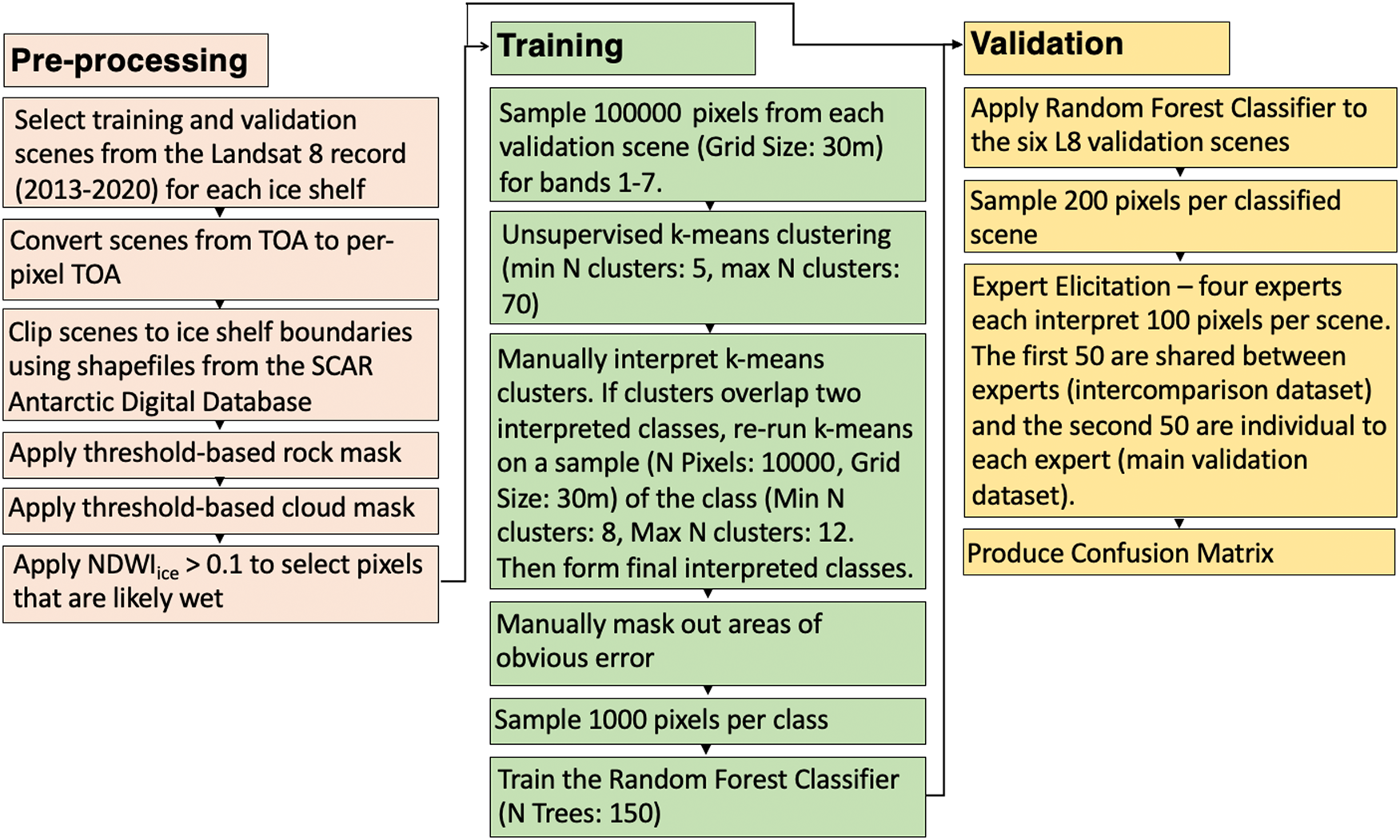
Scenes were pre-processed by converting to per-pixel top-of-atmosphere values (Dell and others, Reference Dell2020), and by clipping to the ice-shelf boundaries (from the SCAR Antarctic Digital Database). A rock mask was then applied to each scene, following the method of Moussavi and others (Reference Moussavi2020). This mask was then buffered by 1 km to ensure full removal of rock and rock shadow from each scene (Halberstadt and others, Reference Halberstadt2020). Clouds (including cirrus) and cloud shadows were identified and masked using the Landsat 8 Quality Assessment Bands, with a 4 km buffer applied to ensure full removal.
Finally, all pixels with an NDWIice > 0.1 were selected for further analysis. We note that in previous studies, to identify slush in addition to shallow and deep water, a threshold of 0.12 has been used (Yang and Smith, Reference Yang and Smith2013; Bell and others, Reference Bell2017). However, in our study, we lowered the NDWIice threshold to 0.1 to include more potentially wet pixels, which were then categorised as ‘slush’, ‘ponded water’ or ‘other’ by the classifier at a later stage. NDWIice was calculated using Landsat 8 bands 2 (blue) and 4 (red):

2.3 Training data generation and supervised classification
To generate training data and to train a supervised classifier, we followed the general methodology of Halberstadt and others (Reference Halberstadt2020), which we briefly summarise here. Training data were generated by applying an unsupervised k-means clustering algorithm (Arthur and Vassilvitskii, Reference Arthur and Vassilvitskii2007) in GEE, which identifies clusters of spectrally distinct pixels across a set of 14 scenes from bands 1–7 (Fig. 3c). The k-means clustering algorithm, which is the only supervised classification algorithm available in GEE, is widely used by the community and is robust, and for these reasons chosen for this study. Initial training data were generated using two image scenes per ice shelf. Our initial trained classifier produced significant misclassification errors over ‘dirty ice’ (i.e. ice that contains debris and/or sediment) regions; the inclusion of two additional Nansen Ice Shelf training scenes added ‘dirty ice’ training data and improved classifier performance.
Example workflow for the k-means clustering algorithm over the Nivlisen Ice Shelf (Landsat 8, 2016-12-27). (a) Base image of the Nivlisen Ice Shelf, the solid black line marks the ice-shelf area (from the SCAR Antarctic Digital Database), the dashed box shows the zoomed area featured in (b), (c) and (d). (b) True colour composite. (c) K-means clusters (shown as different colours). (d) Interpreted ponded water and slush classes, identified from the k-means clusters in (c). In total, ten k-means clusters were combined to form the ponded water class, and ten k-means clusters were combined to form the slush class.

The k-means clustering algorithm was executed by sampling 100 000 pixels from each image at the Landsat 8 native grid size of 30 m. We specified a minimum of 5 and a maximum of 70 clusters when running the k-means clustering algorithm. This maximum value was manually determined, and increasing the value further did not have an impact on the output of the clusterer, as the cluster typically returned no more than ~20 clusters. We then manually interpreted the resulting clusters and grouped them into interpreted classes: ponded water, slush and several others (including, but not limited to, blue ice, snow and dirty ice). The boundary between slush and ponded water was determined by the developer of the classifier, however the transitional and subjective nature of this distinction should be noted, and this boundary is therefore imperfect. In some cases, clusters identified using the k-means algorithm overlapped two interpreted classes. These clusters were therefore further subdivided using k-means (sampling 10 000 pixels at a grid size of 30 m, and specifying a minimum of 8 and maximum of 12 clusters) and the sub-clusters were assigned to an interpreted class. Once the final interpreted classes were formed, areas of mis-classification error were manually masked from the training data. We then randomly sampled 1000 pixels from each interpreted class, to form the final training dataset for all ice shelves combined. These data were then used to train a random forest classifier, implemented in GEE. Random forest classifiers use numerous tree predictors to generate a most-likely outcome (Breiman, Reference Breiman2001). The number of trees for this classifier was set to 150. The relative importance of each band within the random forest classifier was also determined within GEE.
2.4 Validation
The performance of the supervised classifier was validated using the validation dataset, which included one image scene for each of the six study areas. For each of the six validation scenes, the random forest classifier was applied (Fig. 4), and 250 classified pixels were randomly sampled from each scene. We then used expert elicitation (Bamber and Aspinall, Reference Bamber and Aspinall2013), where four glaciologists, who we call ‘experts’, were each asked to manually interpret a total of 100 pixels for each image scene, classifying them as either ‘ponded water’, ‘slush’ or ‘other’. Experts viewed each pixel within its surrounding spatial context, and were permitted to zoom in and out of the image. Furthermore, the experts were all familiar with looking at ice-sheet/-shelf surface hydrology using medium-resolution optical data, and were not directly involved with training the classifier. Experts were not given direction for the interpretation of pixels, to ensure that their interpretations were not biased by the individual who developed the classifier. Of the 100 pixels per image interpreted by each expert, the first 50 pixels for each of the six images were identical. These 300 pixels (the ‘intercomparison dataset’) were used to compare expert opinions to highlight the subjectivity of manually identifying slush and ponded water in satellite imagery. The second 50 pixels per image were unique to each expert, and comprised of the ‘main validation dataset’ (i.e. 1200 pixels in total).
Preliminary outputs from the supervised classifier, as applied to six Landsat 8 validation images for the (a) Nivlisen Ice Shelf, (b) RBIS, (c) Amery Ice Shelf, (d) Shackleton Ice Shelf, (e) Nansen Ice Shelf and (f) George VI Ice Shelf. Panels in column (i) show the pre-processed Landsat 8 RGB images to be classified, with the red boxes delineating close-up areas shown in panels in columns (ii) and (iii). Panels in column (ii) show the close up areas in RGB, and panels in column (iii) show the results for these areas produced by the supervised classifier, with blue = ponded water and green = slush.

For each pixel, in addition to providing an interpretation, each expert assigned a confidence score to reflect the certainty of their manual interpretation. The confidence score values were assigned as either: (1) low-confidence, (2) medium-confidence or (3) high-confidence (Bamber and Aspinall, Reference Bamber and Aspinall2013). These confidence scores provided a way to identify pixels that were likely classified with less accuracy by the experts, due to their uncertainty.
Finally, we present true positives and negatives, as well as false positives (errors of commission) and false negatives (errors of omission) as a confusion matrix (Stehman, Reference Stehman1997) to calculate the classifier accuracy (compared to the expert interpretations) for all pixels, as well as just for the high-confidence pixels. The overall classifier accuracy was calculated by summing all correctly classified pixels (true positive and true negatives) and dividing this sum by the total number of pixels sampled.
2.5 Application on the Roi Baudouin Ice Shelf
Once validated, the classifier was applied to the entire RBIS for Landsat 8 images from 2013 to 2020 to test how well the method upscaled through space and time. We filtered only for images with a solar elevation >20°, but accepted any level of cloud cover in order to utilise as much of the available imagery as possible, thereby increasing data coverage through space and time. These selected images were then pre-processed using the same steps that were applied in the training and validation phases (see Section 2.2). However, rather than processing individual scenes as we did previously, we created 15-day (bi-monthly) mosaiced products from the available scenes to maximise spatial coverage prior to applying the NDWIice > 0.1 filter. Each 15-day mosaiced product was produced using the ‘quality mosaic’ function in GEE, which used the pixel with the greatest NDWIice value for locations where pixels overlapped. For each melt season, the products start on 1 November, and continue in blocks of exactly 15 days until 31 March (or until 1 April for leap years). The supervised classifier was applied to each 15-day product, and the total areas of both slush and ponded water were calculated. For 15-day periods that did not have complete data coverage across the RBIS, we scaled slush and ponded water areas to the full ice-shelf area by calculating the area of slush or ponded water found within each 15-day product as a fraction of the visible ice-shelf area of each 15-day product, and then multiplying this fraction by the full ice-shelf area (Williamson and others, Reference Williamson, Banwell, Willis and Arnold2018; Banwell and others, Reference Banwell2021). In addition to the 15-day products that we exported from GEE, we compiled maximum melt extent maps for each meltseason in MATLAB (Williamson and others, Reference Williamson, Banwell, Willis and Arnold2018) to show each pixel that was covered by either slush, ponded meltwater or both slush and ponded meltwater.
3. Results
3.1 Classification accuracy based on expert elicitation
Table 2 shows the results from the intercomparison dataset for each scene in the validation dataset, which were interpreted by all four experts. The data shown include all interpreted pixels regardless of the associated confidence scores. Overall, the accuracy of the ponded water class is 78%, and the accuracy of the slush class is 71%. For the ponded water class, the experts all produced similar accuracy scores for the RBIS (8% spread), and more dissimilar scores for the Nansen Ice Shelf (30% spread), with a mean spread across all six ice shelves of just 6%. For the slush class, the experts are in the closest agreement over the George VI Ice Shelf (11% spread), and in least close agreement over the Nansen Ice Shelf (79% spread). As with the ponded water class, these discrepancies tend to cancel out between experts giving an overall mean spread across all ice shelves of just 5%. Table 3 shows the same data as Table 2, but only for the pixels for which the experts had ‘high-confidence’ in their interpretation.
Accuracy scores for the intercomparison dataset (the 50 pixels shared by all experts for each ice-shelf validation image), listed by expert

High-confidence accuracy scores for the intercomparison dataset , listed by expert

Table 4 shows the accuracy results for the classifier over the main validation dataset (where each expert interpreted 50 different pixels per ice-shelf). The accuracy for the ponded water class is 78% and for the slush class is 70%; these values are very similar to those produced by the intercomparison dataset. The classifier is most accurate at identifying ponded water for the Shackleton Ice Shelf (91%) and least accurate for the Amery Ice Shelf (61%). In contrast, the classifier is most accurate at identifying slush for the Nivlisen Ice Shelf (80%) and least accurate for the Nansen Ice Shelf (60%). The percentage of low confidence pixels ranges from 13% (Nivlisen and George VI ice shelves) to 28% (the Shackleton Ice Shelf).
Accuracy scores for the main validation dataset (the 200 individual pixels (50 per expert) for each ice-shelf validation image) for the ponded water and slush classes separately. The percentage of pixel confidence scores for each ice shelf are also given.

Table 5 shows the accuracy results for the main validation dataset using high-confidence pixels only. The mean accuracy for the ponded water class is 84% and for the slush class is 82%. Agreement between the experts and the classifier is greatest for ponded water over the Shackleton Ice Shelf (96%) and for slush over the Nivlisen Ice Shelf (92%). This agreement is lowest for ponded water over the Amery Ice Shelf (65%) and for slush over the RBIS (72%).
High-confidence accuracy scores for the main validation dataset for the ponded water and slush classes separately

For the ponded water class, Expert 2 had the lowest agreement with the classifier. This was due to the classifier designating certain pixels as ‘other’ (e.g. non-wet surface facies), whereas the expert interpreted the pixels to be ponded water. For the slush class, Expert 4 had the lowest agreement with the classifier, which classified certain pixels as ‘other’ that were interpreted to be slush by the expert.
3.2 Relative importance of input bands
The relative importance of each band within our supervised classifier was determined within GEE using the ‘.explain()’ function, and the results show that all bands contribute towards the classification of slush and ponded water (Table 6). However, band 5 (near-infrared) is of greatest importance for the supervised classifier, with an importance score of 20% (Table 6). Bands 1–4 (visible) and 6–7 (shortwave infrared 1 and 2) all have similar weightings, with importance scores ranging between 12 and 15%.
Relative importance of each of the Landsat 8 bands used by the supervised classifier

3.3 Application to the Roi Baudouin Ice Shelf
After applying the supervised classifier to the RBIS, two key datasets are produced: a raw (unscaled) dataset and a scaled dataset. The scaled dataset is produced to provide a better estimate of the total ice-shelf surface water area, as for many dates in this study, there is incomplete area-of-interest (AOI) coverage (Fig. 5). Of the 48 15-day periods presented in Fig. 5, 14 have a percentage AOI coverage below 50%. For the remainder of this paper, the scaled values only will be presented, however readers should remain aware of the potential for error when scaling up values across a full ice-shelf, because, for example, unscaled data with incomplete AOI coverage could already represent 100% of the total surface meltwater on the ice-shelf surface. Unscaled data are presented in Fig. S.1.
Time series data for slush and ponded water across the RBIS. Grey bars show the % AOI coverage for each 15-day period plotted. Lines show scaled areas of slush (green line) and ponded water (blue line) on the RBIS from 2013/14 to 2019/20, derived from supervised classification of 15-day Landsat 8 mosaic products created in GEE (see Section 2.5). Data are only plotted where ⩾20% coverage of the RBIS is met. X axis date labels indicate 1 January for each year.

The maximum areas of slush and ponded water are reached between 15 January–29 January 2016 (3.5 × 10⁹ m2) and 30 January–13 February 2017 (1.9 × 10⁹ m2), respectively (Fig. 5). In contrast, the lowest summer maximum areas of slush and ponded water occur between 15 January–29 January 2019 (slush) and 14 February–28 February 2019 (ponded water), reaching values of 5.7 × 10⁸ and 2.9 × 10⁸ m2, respectively. For all seven melt seasons, the total area of slush and ponded water is greatest in either January or February. Furthermore, for all melt seasons except for 2018/19, the greatest areas of slush and ponded water are observed in the same 15-day periods within each melt season. However, for the austral summer of 2018/19, the greatest total area of slush is recorded approximately a month prior to the greatest total area of ponded water (Fig. 5).
Overall, the absolute difference between the greatest areas of slush for each melt season is larger than the absolute difference between the greatest areas of ponded meltwater for each melt season, whereas the percentage change in ponded water is slightly greater than the percentage change in slush. Slush ranges from 5.7 × 10⁸ m2 between 15 January and 29 January 2019, to 3.5 × 10⁹ m2 between 15 January and 29 January 2016 (a 521% change in area), whereas ponded water varies from 2.9 × 10⁸ m2 between 14 February 2019 and 28 February 2019, to 1.9 × 10⁹ m2 between 30 January 2017 and 13 February 2017 (a 559% change in area) (Table S.2). Overall, slush dominates the total meltwater area across the RBIS, making up over half of the total meltwater area on 39 of the 48 15-day periods investigated, and on average accounts for 64% of the total meltwater area (Table S.2). From the 2014/15 melt season onwards, the percentage slush on the RBIS is greatest between 16 November and 30 December, when it accounts for between 84 and 96% of the total meltwater area.
Of the seven melt seasons investigated, the 2016/17 melt season has the greatest recorded total meltwater area, reaching 5 × 10⁹ m2 between 30 January and 13 February 2017. Of this total area, 62% is slush, and 38% is ponded water (Table S.2). Conversely, the melt season that had the lowest total meltwater area is 2019/20, with 7.5 × 10⁸ m2 between 15 January and 29 January 2019. Of that total area, 76% is slush and 24% is ponded water (Table S.2).
Figure 6 shows each of the 15-day data products that were produced within GEE for the 2016/17 melt season over the RBIS. In these 15-day products, we manually inspected each image and ignored errors of commission (false positives) across the central and distal regions of the ice shelf. Therefore, the following results focus on the true positive results for the 2016/17 season, which show meltwater in proximity to the ice shelf's grounding line. Little meltwater is detected between 1 November and 15 December 2016. However, from 16 December to 30 December 2016 onwards, areas of slush begin to develop near the grounding line in both the southeast and central southern parts. By early January (31 December 2016–14 January 2017) ponded water also begins to form among the areas of slush, and the areas of both classes increase until 30 January–13 February 2017, after which the areas of both classes begin to decrease (Figs 5 and 6). A number of the 15-day products for this melt season have data gaps resulting from cloud masking, or a lack of image scenes covering the area of interest. The percentage ice-shelf area coverage by imagery for the 2016/17 melt season ranges from 38% (30 January–13 February 2017) to 99% (1 December–15 December 2016) (Table S.2).
15-day melt products for the 2016/17 melt season across the RBIS. White areas are areas that have either been masked out or were not covered by imagery in the first instance. The red box in the 30 January 2017–13 February 2017 panel roughly denotes the area where errors of commission due to cloud and cloud shadows are generally found.

Data products from GEE were combined in MATLAB to produce maximum melt extents across the RBIS for each melt season (1 November–31 March) from 2013/14 to 2019/20 (Fig. 7). In every melt season, both slush and ponded water are present predominantly in the southeast of the ice shelf, towards the grounding line. This area of slush and ponded water is the most spatially extensive in 2016/17 and 2017/18 (Figs 7d, e), when it extends ~47 km from the grounding line towards the ice-shelf front. In this region, slush is more spatially extensive than ponded water. Ponded water is typically observed towards the northern edge of the melt zone (i.e. closer to the ice front) each year, and is often surrounded by slush (Fig. 7). Between 2013 and 2020, we find that 26% of all pixels that are covered by surface water are covered by both slush and ponded water at least once.
Maximum melt extent plots for each melt season, calculated by mosaicking all 15-day melt products for each melt season in MATLAB. Maximum areas of slush, ponded water and both (where both slush and ponded water are identified within the melt season) are mapped. Red boxes roughly delineate areas affected by data gaps in the 2014/15 and 2018/19 melt seasons.

4. Discussion
4.1 Classifier accuracy
The mean accuracies across all ice shelves of the ponded water and slush classes were 84% and 82%, respectively, when comparing the classifier's outputs to high-confidence expert interpretations (which comprised of 35% of all pixels within the main validation dataset) (Table 5). Over all ice shelves, the percentage of pixels that were classified with high confidence did not exceed 50% (Table 4), highlighting that even ‘experts’ are unable to classify all pixels with total confidence. Thus, although we use expert opinion to assess the accuracy of our classifier, each expert may be no more accurate than the classifier output itself. A solution to this would be to use ground-based multi- or hyper-spectral data from ice shelves as ground truth data. However, to the authors' knowledge, no such data currently exist.
By collecting four expert interpretations, we aimed to minimise the effects of bias that each expert may have, and to get a more holistic set of expert interpretations for each ice-shelf. The need for this approach was indicated by the spread between high-confidence pixels classified by experts for each ice-shelf in the intercomparison dataset (Table 3). For example, on the Nansen Ice Shelf, agreement between the experts and the classifier ranged from 50 to 100% for ponded water, and from 25 to 86% for slush. Although the accuracy assessment attempts to best mimic ground-truthing through the use of multiple experts, it should be noted that the classifier is trained predominantly by a single person (separate to the experts used to validate the classifier), and so the classifier may reflect the biases of that individual. In addition, although experts are able to interpret a pixel within its surrounding spatial context, including both the immediate surrounding pixels as well as those elsewhere on the ice-shelf, the classifier assesses the spectral characteristics of the pixel alone. This difference could be overcome by using object-based image analysis, however Halberstadt and others (Reference Halberstadt2020) found such methods had a lower overall accuracy in comparison with pixel-based methods for the classification of ponded water. In the future, research should look at collecting ground-based multi- or hyper-spectral data across ice shelves, which would facilitate a more robust assessment of this classifier's accuracy.
As previously mentioned, the main validation dataset for high-confidence pixels returned accuracy scores of 84% for ponded water and 82% for slush. Similar research for supervised classification of surface lakes only (i.e. not including slush) on Antarctic ice shelves achieved a mean pixel-based accuracy score of 93% (Halberstadt and others, Reference Halberstadt2020). Our slightly lower scores likely reflect the incorporation of slush into the classifier, in addition to the fact that we used a wider range of training sites. Furthermore, our validation techniques were different, as we validated the classifier against multiple expert opinions, as opposed to just one expert in Halberstadt and others (Reference Halberstadt2020).
In our study, agreement between the classifier and the expert interpretations for high-confidence pixels was greatest for ponded water over Shackleton (96%) and for slush over Nivlisen (92%). However, the classifier accuracy was lowest over Amery, achieving 65% accuracy for ponded water and 73% for slush. The majority of the classification errors on the Amery Ice Shelf in particular appear to have resulted from topographic shadows being incorrectly classified as either slush or ponded water (Fig. 4). Additionally, on the validation image for the Amery Ice Shelf, there were examples of ponded water covered by a thin ice layer (Fig. 4). The classifier tended to classify these areas as slush, as the thin ice layer adjusted the spectral properties of each pixel, whereas the experts differed in their interpretations and often interpreted them as ponded water or other.
Another source of classifier error was subjectivity when defining the slush/ponded-water boundary. Although the classifier utilised training data to determine the slush/ponded-water boundary, comparing classifier results with expert interpretations revealed some disagreement. However, we note that this disagreement is likely no greater than disagreement between the experts themselves, resulting from individual subjectivity, as neither the experts nor the classifier were consistently more or less conservative when marking the slush/ponded-water boundary. Again, considering future research, without ground-based multi- or hyper-spectral data it would be difficult to further improve such estimations of the slush/ponded-water boundary.
A final source of classifier-error was errors of commission resulting from cloud and cloud shadows and this is discussed separately in Section 4.4.
4.2 Comparison to NDWIice
Although threshold-based methods have been used for the identification of deep surface meltwater bodies (e.g. surface lakes and streams) on Antarctic ice shelves (e.g. Banwell and others, Reference Banwell2014; Bell and others, Reference Bell2017; Kingslake and others, Reference Kingslake, Ely, Das and Bell2017; Stokes and others, Reference Stokes, Sanderson, Miles, Jamieson and Leeson2019; Dell and others, Reference Dell2020; Moussavi and others, Reference Moussavi2020), no prior studies have also attempted to map slush across an entire ice-shelf for multiple melt seasons. Upscaling slush identification through space and time using simple threshold-based mapping approaches would lead to significant errors of omission and commission, owing to the spectral similarities between slush and other surface facies (e.g. lakes, blue ice and dirty ice) (Fig. 8). For example, we found that applying NDWIice thresholds of >0.12 and ⩽0.14 for slush and >0.14 for ponded water (following Yang and Smith, Reference Yang and Smith2013 and Bell and others, Reference Bell2017) over the Shackleton Ice Shelf led to large errors of omission for slush when compared to the classifier output, due to confusion between ponded water and slush (Fig. 8). In contrast, applying these NDWIice thresholds over the Nansen Ice Shelf led to errors of commission for slush, due to confusion between blue ice and slush (Fig. 8). On the George VI Ice Shelf, however, the differences between the threshold method and the classifier output were small, although even here the threshold method tended to underestimate slush area compared to the classifier (Fig. 8).
Outputs from the supervised classifier and from NDWIice thresholding applied to sections of the validation images (as shown in Fig. 4) for Shackleton, Nansen and George VI ice shelves. Panels show the base RGB images, the area classified using the supervised classifier developed in this study and the area classified using NDWIice thresholds, where slush is >0.12 and ⩽ 0.14 and ponded water is > 0.14.

The limitations of the NDWIice method that we have described above were overcome through our supervised classifier, as it was trained using seven Landsat 8 bands (bands 1–7) as opposed to just two (bands 2 and 4) for NDWIice, and it was therefore better able to distinguish between surface classes using a broader range of spectral information. For our classifier, the near infrared band (band 5) was found to be the most important when distinguishing between classes (Table 6). This is likely related to the low reflectivity of water in near-infrared wavelengths (Work and Gilmer, Reference Work and Gilmer1976; Yang and others, Reference Yang, Wang, Zhao and Guo2011). Overall, although simple threshold-based methods seem capable of accurately classifying ponded meltwater on ice shelves, classifying surface facies such as slush, which have similar spectral properties to much of their surroundings, requires more spectral information. Although threshold-based approaches do not exclude the use of more spectral information, the manual selection of each threshold is arduous. ML overcomes this as it is able to determine which spectral information is of value for each classification based upon the training data.
4.3 Evolution of slush and ponded water over the Roi Baudouin Ice Shelf
To demonstrate the potential of our supervised classifier for pan-Antarctic identification of slush and ponded water over time, we applied it across the RBIS for the Landsat 8 images between 2013 and 2020. Of the seven melt seasons investigated (2013/14 to 2019/20), the greatest total meltwater extent (5.0 × 10⁹ m2) was recorded between 30 January and 13 February 2017. This observation is broadly corroborated by Halberstadt and others (Reference Halberstadt2020) who classified surface lakes on the RBIS over a number of image scenes between 2013 and 2018, and found peak melt area on the 25th February 2017. Furthermore, our findings align with studies on the Amery Ice Shelf, where threshold-based methods (Moussavi and others, Reference Moussavi2020) and ML methods (Halberstadt and others, Reference Halberstadt2020) were used to calculate the area of surface lakes over a single path/row. Similarly to Moussavi and others (Reference Moussavi2020), although we identified marked inter-annual variability in both slush and ponded water areas, we found the intra-seasonal trends for inferred meltwater storage to be fairly consistent.
As slush (which may be saturated firn or saturated snow overlying blue ice, refrozen lakes, or extensive ice layers of refrozen previously infiltrated water) accounted for an average of 64% of the total meltwater area on the RBIS over the full study period, our findings highlight the importance of accurately mapping slush extent in addition to ponded water extent when investigating surface meltwater on Antarctic ice shelves. Most research until this point has focused on meltwater stored in surface lakes, owing to their significance for potential hydrofracture-induced ice-shelf collapse. For example, a study by Stokes and others (Reference Stokes, Sanderson, Miles, Jamieson and Leeson2019) identified >1300 km2 of surface meltwater held in surface lakes across East Antarctica in January 2017. Based on our findings, in January 2017, the mean proportion of slush on the RBIS was 59%. Although the proportion of slush on other East Antarctic ice shelves has not yet been quantified, our observations of the proportion of slush across the RBIS highlight the need to account for slush when calculating total surface meltwater areas, and it is likely that the total area of meltwater across East Antarctica far exceeds the 1300 km2 of ponded meltwater that has been reported by Stokes and others (Reference Stokes, Sanderson, Miles, Jamieson and Leeson2019).
We found that the proportion of slush relative to ponded meltwater across the RBIS was greatest between 16 November and 30 December each melt season (excluding 2013/14, when it was greatest between 15 January and 29 January 2014). Although no previous literature has mapped the extent of slush on an interannual timescale, Bell and others (Reference Bell2017) used a simple NDWIice threshold to identify slush on a small area of the Nansen Ice Shelf in the 2013/14 melt season. They found the area of slush was greatest on 26th December 2013 and then gradually declined throughout early January 2014 (Bell and others, Reference Bell2017). Although this trend contradicts our findings for the 2013/14 season on the RBIS, it corroborates the trends we identify through the remaining six melt seasons (2014/15 to 2019/20). Bell and others (Reference Bell2017) suggested that the expansive slush identified on the Nansen Ice Shelf in December coalesced to form ponded meltwater by early January. We propose that a similar transition occurred across the RBIS, as the percentage of the total meltwater on the ice–shelf held in slush generally fell from the end of December and into early January, and an increasing amount of melt was therefore held in water bodies.
For surface meltwater to pond, the underlying surface needs to be impermeable, and is likely, therefore, to be either blue ice or saturated firn (slush). Based on the results presented here (Fig. 7) many pixels that are classified as ponded water are also classified as slush at least once in the melt season. Over the full study period (2013–2020), 26% of all water-covered pixels are occupied by slush and ponded water at least once. In these locations, therefore, it is likely that as melt increases throughout the melt season, the firn layer becomes increasingly saturated and water can no longer percolate into the firn pack, which results in ponding at the surface, and lateral transfer of meltwater across the ice shelf surface. However, we also note that some pixels are classified as only ponded water during a melt season, and were therefore not preceded by slush (Fig. 7). Evidence for this is seen in all melt seasons and is particularly prominent towards the central grounding line. We postulate that these areas of ponded water are filling depressions within blue ice surfaces or are forming on top of melt ponds which may have refrozen.
Exposed blue ice surfaces have been identified previously in proximity to the Roi Baudouin grounding line, and result from katabatic winds which cause snow erosion and an increase in near-surface temperatures as winds cause mixing in the stable boundary layer and adiabatic warming (Vihma and others, Reference Vihma, Tuovinen and Savijärvi2011; Lenaerts and others, Reference Lenaerts2017). Lenaerts and others (Reference Lenaerts2017) attributed a doubling in summer surface melt at the grounding line to the katabatic winds, and they also noted that the exposed blue ice surfaces will contribute to further melt, as they have a lower surface albedo than snow-covered surfaces. These processes help to explain the main patterns of ponded meltwater that we observe across the RBIS, as ponded meltwater is clustered near to the grounding line (Figs 6 and 7).
4.4 Errors arising from cloud and cloud shadows
In both the validation dataset and the larger Roi Baudouin dataset, errors of commission due to cloud and cloud shadows are evident (Figs 4–6), which highlights a limitation of our classifier. For example, from 31 December 2016 to 14 January 2017, and through to the end of the melt season, errors of commission are identified over the central and distal regions of the RBIS (e.g. see red panel in Fig. 6). Similar errors are identified within the maximum melt extent products (Fig. 7). This limitation has also been found in similar previous research (e.g. Halberstadt and others, Reference Halberstadt2020), with errors resulting from imperfect cloud-masking methods.
The transient nature of cloud and cloud shadows mean that these errors of commission will have a low persistence over entire melt seasons. This is demonstrated in Fig. 9, which shows the number of times over the full study period that a pixel is classified as either slush or ponded water over the RBIS. The errors of commission in the central and distal regions of the ice-shelf have a persistence score of one (Fig. 9, grey pixels), meaning that each pixel was classified as water at only a single point in time. In contrast, areas of extensive meltwater towards the southeast and central southern grounding line generally have higher persistence values (Fig. 9). Therefore, a potential solution to errors of commission resulting from cloud and cloud shadows when looking at maximum melt products for each melt season would be to filter out pixels with a persistence of one. However, this would lead to the removal of some true positives, where water has been correctly classified at its maximum extent for the melt season, but for only a single point in time. Future research is needed to develop methods to reduce the errors of commission introduced by clouds, either at the pre-processing stage prior to classifier development, or post classifier application. Meanwhile, our maximum melt extents (Fig. 7) are likely to be overestimates.
Heatmap showing the number of times (i.e. persistency scores) each pixel is classified as (a) slush, (b) ponded water and (c) either slush or ponded water over all of the 15-day products produced for the full study period (2013–20).

5. Conclusions
We have presented an ML method that is capable of accurately classifying slush and ponded water across Antarctic ice shelves using the Landsat 8 record from 2013 to 2020. This is achieved by using a random forest classifier, which is trained using spectral data from six different ice shelves around the continent. The classifier performs well across all ice shelves throughout multiple melt seasons, achieving mean accuracies of 84% for ponded water and 82% for slush. Although the classifier encounters errors when defining the slush/ponded-water boundary, we also find that experts disagree on where this boundary should lie, and it is therefore likely that the extent of slush cannot be more accurately mapped without the collection of ground-truthed data. Errors of commission caused by cloud and cloud shadows are the main source of error associated with this method. Future research should look at improving cloud-masking approaches before applying the classifier, or developing a means of filtering out false positives caused by clouds after the classifier has been applied. In this way, it will be possible to produce accurate time series of slush and ponded meltwater extents across all Antarctic ice shelves.
Finally, we applied the classifier to the RBIS for the 2013/14 to 2019/20 melt seasons in order to produce a time series of slush and ponded melt extent. For each melt season, many of the pixels classified as ponded water were also classified as slush; an observation that likely captures the saturation of firn and subsequent formation of surface ponds as the melt season progresses. On average slush accounted for around two-thirds of the total meltwater extent. This highlights the need to map slush in addition to ponded water on ice shelves over a pan-Antarctic scale, to ensure we do not underestimate the area of surface meltwater. The accurate time series data produced by this method, which captures all surface meltwater across Antarctic ice shelves should be used to validate and improve surface mass-balance models.
Supplementary material
The supplementary material for this article can be found at https://doi.org/10.1017/jog.2021.114
Acknowledgements
We thank Mahsa Moussavi for her guidance throughout this project. Rebecca L. Dell was funded by a Natural Environment Research Council (NERC) Doctoral Training Partnership Studentship (CASE with the British Antarctic Survey, grant no. NE/L002507/1). Alison F. Banwell received support from the U.S. National Science Foundation (NSF) under award no. 1841607 to the University of Colorado Boulder. Ian Willis was supported by the UK Natural Environment Research Council under NE/T006234/1 awarded to the University of Cambridge.
Data availability
Ice-shelf boundaries were downloaded from the SCAR Antarctic Digital Database. Key code is available in the Apollo – University of Cambridge Repository (https://doi.org/10.17863/CAM.77156). Please note that as the code is run in Google Earth Engine, extremely minor differences may occur between runs, due to floating point errors.


 Open access