


Introduction
Wildlife viewing is an important yet often underappreciated ecosystem service. Recent national surveys indicate that it has widespread appeal, with over half of U.S. residents engaging in viewing-associated activities annually, which range from backyard bird watching to maintaining land to benefit wildlife (USDOI 2022). Recreational interactions like these contribute to well-being in ways measurable through nonmarket valuation techniques. Such information about economic values can complement wildlife value orientation scales (e.g., assessing mutualism versus utilitarianism) traditionally used by decision-makers to assess the social consequences of management strategies (Fulton et al. Reference Fulton, Manfredo and Lipscomb1996; Manfredo et al. Reference Manfredo, Teel and Bright2003; Teel and Manfredo Reference Teel and Manfredo2010).
The goal of this paper is to address a persistent challenge in the nonmarket valuation of wildlife viewing. Many wildlife populations are mobile because animals can move from one site to another. Consequently, disturbances or management changes targeted at one site can alter conditions at other sites, resulting in a mix of direct and incidental welfare effects. Such changes can arise due to hunting and habitat loss. Hunting pressure can push populations into non-hunting areas, and habitat loss can lower populations in surrounding sites (Newbold and Massey Reference Newbold and Massey2010; Sanchirico and Wilen Reference Sanchirico and Wilen2001). Basic welfare calculation simulates changes at one or more policy sites without accounting for indirect changes elsewhere. While this may be appropriate for site attributes that lack spillover effects, valuing wildlife requires a more sophisticated approach to modeling and valuation.
This paper examines the role of wildlife mobility in nonmarket valuation using a coupled system of recreation demand and wildlife connectivity. The models in this system allow us to structurally identify the welfare effect of a disturbance at a policy site while accounting for connectivity. Wildlife spatially adjust, or sort, to a new equilibrium, which in turn affects wildlife viewers. This stands in contrast to the basic approach that ignores adjustments that occur away from the policy site. We compare the effects of various disturbances using coupled and uncoupled models in order to shed light on the amount of bias that arises from ignoring connectivity.
This paper makes two contributions to the nonmarket valuation literature. First, it examines how changes in wildlife abundance affect recreation demand in the context of spillovers. Little prior research accounts for spillovers beyond visitor substitution effects, despite evidence that ignoring ecological connectivity can introduce substantial bias (Newbold and Massey Reference Newbold and Massey2010). Second, our investigation focuses on values for wildlife abundance using revealed preference data. In contrast, most prior studies leverage measures of hypothetical abundance generated from choice experiments (Aanesen et al. Reference Aanesen, Armstrong, Czajkowski, Falk-Petersen, Hanley and Navrud2015; Armstrong et al. Reference Armstrong, Aanesen, van Rensburg and Sandorf2019; Lew et al. Reference Lew, Layton and Rowe2010; Myers et al. Reference Myers, Parsons and Edwards2010) or simple presence-absence indicators (Boyle Reference Boyle1989; Kolstoe and Cameron Reference Kolstoe and Cameron2017; Navrud and Mungatana Reference Navrud and Mungatana1994), though there are exceptions (Melstrom et al. Reference Melstrom, Lupi, Esselman and Stevenson2015). Our application measures local abundance using seasonal visitor observations across a large number of sites. The granularity of this data allows the analysis to shed light on the degree to which values scale with changes in abundance.
We parameterize the system using data from the eBird project. This application extends prior research on the value of birding (e.g., Jayalath et al. Reference Jayalath, Lloyd-Smith and Becker2023; Kolstoe and Cameron Reference Kolstoe and Cameron2017) by explicitly accounting for connectivity. We find that a 50% reduction in sandhill cranes at state wildlife areas in Indiana results in an annual loss of about $79,000 based on an uncoupled system and $60,000 or $72,000 in the coupled system, depending on how we model connectivity. This implies that research ignoring ecological connectivity could overestimate losses by as much as one-third. Our policy simulations also confirm the importance of presence-absence measures used in prior work: we show that willingness to pay to avoid losses increases substantially when the local abundance of a species moves from partial loss to complete elimination.
A coupled system of recreation demand and wildlife connectivity
This section describes our approach to modeling wildlife viewing and connectivity. We begin by constructing a conventional random utility maximization (RUM) model of recreational behavior. We then develop a model of connectivity to link what visitors see at viewing sites to wildlife mobility. Site choice decisions are a function of two population distributions – people and animals – which policy actions can “disturb.” Modelling connectivity in this way allows us to structurally identify the effects of local but mobile wildlife abundance on recreation demand. After parameterizing the models with an application to birding, we consider scenarios that disturb conditions at a set of policy sites to varying degrees, which consequently alters the equilibrium distribution of wildlife across the entire study region.
The RUM model takes the form ${U_{ij}} = \gamma {a_j} + \beta {x_j} - \rho t{c_{ij}} + {\epsilon _{ij}}$
where ${a_j}$
is local wildlife abundance,
${a_j}$
is local wildlife abundance, ${x_j}$
accounts for other site-specific attributes,
${x_j}$
accounts for other site-specific attributes, $t{c_{ij}}$
is the cost of traveling from residential location i to site j, and
$t{c_{ij}}$
is the cost of traveling from residential location i to site j, and ${\epsilon _{ij}}$
is the error. If individuals choose the site with the most utility and
${\epsilon _{ij}}$
is the error. If individuals choose the site with the most utility and ${\epsilon _{ij}}$
is distributed Type I extreme value, then the probability of choosing site j is
${\epsilon _{ij}}$
is distributed Type I extreme value, then the probability of choosing site j is ${P_{ij}} = {{{e^{\gamma {a_j} + \beta {x_j} - \rho t{c_{ij}}}}} \over {\sum\nolimits_{k = 1}^{J + 1} {{e^{\gamma {a_k} + \beta {x_k} - \rho t{c_{ik}}}}} }}$
where $J + 1$
includes
$J + 1$
includes $J$
sites plus the option to stay home. We index the stay-home option as site J + 1.
$J$
sites plus the option to stay home. We index the stay-home option as site J + 1.
We approach wildlife connectivity through the framework of an equilibrium sorting model. Individual animals are mobile but find it optimal make a single “site choice” until habitat conditions change. This decision is not random; all else equal, we expect that animals prefer locations that support a high survival rate. Suppose that utility for animal l takes the form $U_{lj}^W = {\delta _j} + {\eta _{lj}}$
where ${\delta _j}$
is an index that converts habitat quality to a measure of the average benefit of site j and
${\delta _j}$
is an index that converts habitat quality to a measure of the average benefit of site j and ${\eta _{lj}}$
is an idiosyncratic benefit specific to animal l and site j. Animals that move from site A to B experience a change of utility given by
${\eta _{lj}}$
is an idiosyncratic benefit specific to animal l and site j. Animals that move from site A to B experience a change of utility given by $U_{lB}^W - U_{lA}^W = {\delta _B} - {\delta _A} - \mu dis{t_{AB}} + {\eta _{lB}} - {\eta _{lA}}$
where $dis{t_{AB}}$
is the distance between A and B. The idea here is that moving is costly because it requires expending energy, which animals will trade off with habitat quality at rate
$dis{t_{AB}}$
is the distance between A and B. The idea here is that moving is costly because it requires expending energy, which animals will trade off with habitat quality at rate $\mu $
. If
$\mu $
. If ${\eta _{lj}}$
is distributed Type I extreme value, then the probability of moving takes the form
${\eta _{lj}}$
is distributed Type I extreme value, then the probability of moving takes the form $P_B^W = {{{e^{{\delta _B} - {\delta _A} - \mu dis{t_{AB}}}}} \over {\sum\nolimits_{k = 1}^J {{e^{{\delta _k} - {\delta _A} - \mu dis{t_{ak}}}}} }}\forall k \in \left\{ {1, \ldots, J} \right\}$
This probability is analogous to the survival function that Newbold and Massey (Reference Newbold and Massey2010) use to characterize mobile wildlife. If local abundance is ${a_l}$
, then the resulting population change takes the form
${a_l}$
, then the resulting population change takes the form ${a_B} = \sum\nolimits_A^J {{{{e^{{\delta _B} - {\delta _A} - \mu dis{t_{AB}}}}} \over {\sum\nolimits_{k = 1}^J {{e^{{\delta _k} - {\delta _A} - \mu dis{t_{Ak}}}}} }}} {a_A}.$
In equilibrium, local abundance is the fixed point of the system implied by Equation (6).
We consider two possible parameterizations of Equation (6). First, we set $\mu $
to zero and
$\mu $
to zero and ${\delta _j} = {\rm{ln}}\left( {{a_j}} \right)$
. Not only is
${\delta _j} = {\rm{ln}}\left( {{a_j}} \right)$
. Not only is ${a_j}$
likely a good proxy for habitat quality, but this functional specification also means that the predicted distribution from Equation (6) collapses to the status quo distribution, i.e. animals prefer the current local abundance equilibrium. This parameterization, however, turns off the role that distance can play in connectivity. Therefore, we also consider a specification in which
${a_j}$
likely a good proxy for habitat quality, but this functional specification also means that the predicted distribution from Equation (6) collapses to the status quo distribution, i.e. animals prefer the current local abundance equilibrium. This parameterization, however, turns off the role that distance can play in connectivity. Therefore, we also consider a specification in which $\mu = 1$
,
$\mu = 1$
, $dis{t_{AB}}$
is measured in miles, and
$dis{t_{AB}}$
is measured in miles, and ${\delta _j}$
is the solution to a contraction mapping that produces
${\delta _j}$
is the solution to a contraction mapping that produces ${a_B} = {a_A}$
. The contraction mapping produces a parameterization in which the predicted distribution in equilibrium again collapses to the observed distribution.
${a_B} = {a_A}$
. The contraction mapping produces a parameterization in which the predicted distribution in equilibrium again collapses to the observed distribution.
Distance is an important component in connectivity analysis, and we acknowledge that the relationship between distance and wildlife mobility is probably more complex than Equation (6). The relationship could be nonlinear, or linear but weaker than we assume. Comparing welfare estimates across coupled and uncoupled systems, though, sheds light on the sensitivity of the results to alternative ways of modeling the effect of distance. We show that the distance-adjusted connectivity model produces welfare estimates that fall between two bounds: those from the coupled system with no distance effect and the uncoupled system that ignores connectivity altogether. This bounding indicates that our qualitative conclusions would remain unchanged with a more complex distance-based connectivity analysis.
Using the estimates from the RUM and wildlife connectivity models, the formula measuring willingness to pay (WTP) for a change in local abundance is $WT{P_i} = {{\ln \left( {\sum\nolimits_j {{e^{\gamma {a_j} + \beta {x_j} - \rho t{c_{ij}}}}} } \right) - \ln \left( {\sum\nolimits_j^{} {{e^{\gamma a_j^* + \beta {x_j} - \rho t{c_{ij}}}}} } \right)} \over \rho }$
where $a_j^*$
measures local abundance after the disturbance. The average WTP across all choice occasions in the sample is
$a_j^*$
measures local abundance after the disturbance. The average WTP across all choice occasions in the sample is $\overline {WTP} = \mathop \sum \nolimits_{i = 1}^N WT{P_i}/N\;$
, where
$\overline {WTP} = \mathop \sum \nolimits_{i = 1}^N WT{P_i}/N\;$
, where $N$
is the sample size. One can calculate the total welfare change in the study area as
$N$
is the sample size. One can calculate the total welfare change in the study area as $TWTP = \overline {WTP} \times \left( {\mathop \sum \nolimits_{j = 1}^{J + 1} visit{s_j}} \right)$
, where
$TWTP = \overline {WTP} \times \left( {\mathop \sum \nolimits_{j = 1}^{J + 1} visit{s_j}} \right)$
, where $\mathop \sum \nolimits_{j = 1}^{J + 1} visit{s_j}$
is the number of choice occasions in the population. In the application below, we calculate the welfare effects of hypothetical disturbances involving 5%, 10%, 25%, 50%, 95% and 100% reductions in abundance at selected sites.
$\mathop \sum \nolimits_{j = 1}^{J + 1} visit{s_j}$
is the number of choice occasions in the population. In the application below, we calculate the welfare effects of hypothetical disturbances involving 5%, 10%, 25%, 50%, 95% and 100% reductions in abundance at selected sites.
Application
This section describes an application of the coupled system to birding, which is the most popular wildlife viewing activity in the United States. Away-from-home birders average 34 days of birding annually, making them avid travelers (USDOI 2022). Birding has been the subject of several valuation studies (Jayalath et al. Reference Jayalath, Lloyd-Smith and Becker2023; Kolstoe and Cameron Reference Kolstoe and Cameron2017; Roberts et al. Reference Roberts, Devers, Knoche, Padding and Raftovich2017). Melstrom et al. (Reference Melstrom, Nielsen and Reeling2024) estimates WTP for changes in sandhill crane (Antigone canadensis) abundance at three sites in Indiana. We extend this work by including connectivity effects and expanding the study area to sites across Indiana.
Background
Indiana provides a useful setting to study wildlife population spillovers. The state lies within the Mississippi Flyway, a major migration route running from Canada to the Gulf of America (Gulf of Mexico), and hosts a mix of permanent and migratory species. Birders have access to several hundred local, state, and federal parks, which often permit hunting, such as in state wildlife areas. Evidence indicates that hunting disturbs and redistributes bird populations. Migratory birds tend to avoid permitted hunting areas, leading to lower densities relative to protected sites (Dinges et al. Reference Dinges, Webb and Vrtiska2015; Madsen and Fox Reference Madsen and Fox1995). This redistribution reduces birding opportunities at hunting sites while potentially increasing them elsewhere.
State wildlife managers believe that hunting pressure leads to migratory-induced population shifts that are more pronounced than the actual losses from harvest. For a species like the currently protected sandhill crane, managers anticipate minimal reductions if the state decides to allow hunting. Neighboring Kentucky’s sandhill crane harvest program has remained modest since its 2011 inception, averaging just 857 hunting tags and 101 birds annually (Seamans Reference Seamans2023). Indiana is home to several key stopping points and viewing areas for sandhill cranes (Greene Reference Greene2020; Zorn Reference Zorn2021). Birders value the birds’ large size, loud calls, and large flocks, which can number in the thousands. Consequently, managers’ primary concern is that hunting would disturb viewing opportunities around popular wildlife areas. Our estimates reveal the potential welfare consequences of reductions in local crane abundance at these sites.
Data
Our application relies on eBird, a community science project that monitors bird species developed and managed by the Cornell Lab of Ornithology. Amateur and professional volunteers use eBird’s mobile phone application to describe bird sightings in the form of checklists, which they submit after a site visit known as a “sampling event.” Checklists record the species volunteers identify by sight or sound. Anonymized checklist data is publicly available and contains the name of identified species, number observed, location, date, travel protocol, personal identifier, group identifier if the volunteer was part of a group, and a sampling event ID code. For additional details on the eBird database, see Sullivan et al. (Reference Sullivan, Aycrigg, Barry, Bonney, Bruns, Cooper, Damoulos, Dhondt, Dietterich, Farnsworth, Fink, Fitzpatrick, Fredericks, Gerbrach, Gomes, Hochachka, Iliff, Lagoze, La Sorte, Merrifield and Kelling2014).
We narrow the data to sampling events at public “hotspots” in Indiana. eBird recommends grouping hotspots in close proximity because they are often simply different habitats (e.g., fields, forests) in the same named location. Interviews with eBird users confirm that many hotspots are not interpreted as distinct sites. We group hotspots that share a common name and management authority. An exception are hotspots that share a name and management authority but are located in different counties, which we separated in order to minimize aggregation bias (Parsons and Needelman Reference Parsons and Needelman1992). This approach prevents artificially grouping geographically distinct locations that visitors perceive as different sites due to distance. We measure visitation by counting the number of sampling events in 2021 and 2022, each divided into two periods, which includes fall migration (September–December) and rest-of-year (January–August). We separate fall migration from rest-of-year because birding and particularly sandhill crane viewing is more popular in the fall (A. Phelps, Indiana DNR, personal communication). These counts include only sampling events that submitted a checklist indicating that the trip was taken primarily for the purpose of birding. Figure 1 maps birding sites and total visits (from 2021 and 2022) in the data.
Public birding sites and hunting lands in Indiana.

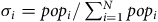
We construct several bird-related site attributes (Table 1). This includes a count of all species (species richness), a count of species of state concern, and one count each of species in the Gruiformes (which includes cranes) and Anatidae (which includes ducks and geese) taxonomic orders. We also include measures of local abundance for sandhill cranes, mallards (Anas platyrhynchos), and snow geese (Anser caerulescens). Our policy scenarios focus on changes in crane abundance. Mallards and snow geese serve as controls in the model to address concerns that crane abundance correlates with other migratory birds.
Summary statistics of Indiana bird watchers and site attributes

Attribute statistics calculated using 756 sites derived from eBird hotspots across four seasons in 2021 and 2022. The number of site observations is 2,499 after filtering out sites with zero visits.
We measure local abundance conditional on individual checklist characteristics. This is important because reported bird counts can vary from person to person due to differences in time on site, time of day, etc., making the counts susceptible to individual error. To account for this error, we follow Liang et al. (Reference Liang, Rudik, Zou, Johnston, Rodewald and Kling2020) and model abundance according to $\ln \left( {{b_{jtrh}}} \right) = {\beta _0} + {\beta _1}hour{s_{jtr}} + {\beta _2}protoco{l_{jtr}} + {\beta _3}observer{s_{jtr}} + {\zeta _h} + {{\rm{\Gamma }}_{jt}} + {\epsilon _{jtr}}$
where ${b_{jtrh}}$
is the number of birds reported at site j in season t by individual r at time h. The right-hand side includes trip duration (
${b_{jtrh}}$
is the number of birds reported at site j in season t by individual r at time h. The right-hand side includes trip duration ( $hour{s_{jtr}}$
), the purpose of the trip (
$hour{s_{jtr}}$
), the purpose of the trip ( $protoco{l_{jtr}}$
), the number of observers (
$protoco{l_{jtr}}$
), the number of observers ( $observer{s_{jtr}}$
), and hourly fixed effects (
$observer{s_{jtr}}$
), and hourly fixed effects ( ${\zeta _h}$
) for time of day. We use the site-by-season fixed effects as the measure of local abundance (i.e.
${\zeta _h}$
) for time of day. We use the site-by-season fixed effects as the measure of local abundance (i.e. ${{\rm{\Gamma }}_{jt}} \equiv {a_{jt}}$
) in the RUM and connectivity models.
${{\rm{\Gamma }}_{jt}} \equiv {a_{jt}}$
) in the RUM and connectivity models.
Next, we calculate travel costs between residential locations and sites according to $t{c_{ij}} = 2\left[ {mc \times dis{t_{ij}} + {1 \over 2} \times \left( {incom{e_i}/2000} \right) \times t{t_{ij}}} \right]$
where $mc$
is a per-mile driving cost,
$mc$
is a per-mile driving cost, $dis{t_{ij}}$
is distance and
$dis{t_{ij}}$
is distance and $t{t_{ij}}$
is travel time, and
$t{t_{ij}}$
is travel time, and $\left( {incom{e_i}/2000} \right) \times t{t_{ij}}/2$
measures the value of travel time (VOTT). We use AAA’s Your Driving Cost report to calculate
$\left( {incom{e_i}/2000} \right) \times t{t_{ij}}/2$
measures the value of travel time (VOTT). We use AAA’s Your Driving Cost report to calculate $mc$
by subtracting the average cost of driving 10,000 miles from the cost of driving 15,000 miles and then dividing by 5,000. This calculation implicitly accounts for fuel and mileage-related depreciation. We measure distance and travel time using the fastest driving route. We use ZIP codes for residential locations and calculate VOTT by dividing the median household income in a ZIP code by 2,000 multiplied by one-half, which assumes working 2,000 hours in a year and that travel time is valued at one-half the wage rate. We also present estimates with VOTT set at one-third the wage rate.
$mc$
by subtracting the average cost of driving 10,000 miles from the cost of driving 15,000 miles and then dividing by 5,000. This calculation implicitly accounts for fuel and mileage-related depreciation. We measure distance and travel time using the fastest driving route. We use ZIP codes for residential locations and calculate VOTT by dividing the median household income in a ZIP code by 2,000 multiplied by one-half, which assumes working 2,000 hours in a year and that travel time is valued at one-half the wage rate. We also present estimates with VOTT set at one-third the wage rate.
To extrapolate the welfare loss in the eBird sample to the Indiana population per year, we estimate annual away-from-home birding trips using the 2022 National Survey of Fishing, Hunting, and Wildlife-Associated Recreation’s (NSFHWAR) estimate of 257 million days in the United States, assuming all trips are day trips and that 2% of these occur in Indiana, which is proportional to population. We then reduce the estimate by 50% to account for the fact that only half of birding activity occurs at hotspots based on proportions in the eBird sample.
Estimation
This section describes our approach to estimating the RUM model. The conventional approach uses conditional logit regression and individual choice data (Haab and McConnell 2002). We, however, use a mathematical technique to leverage aggregate choice data (Melstrom and Reeling Reference Melstrom and Reeling2024). This approach is necessary because individual-level trips are unavailable in the eBird data due to the suppression of home addresses. Researchers who want to develop a similar coupled model in other contexts can choose the conventional individual-level approach, our aggregate approach, or some other method depending on data availability and research objectives.
We begin by constructing visitation shares ${s_j} = {{visit{s_j}} \over {\sum\nolimits_{j = 1}^{J + 1} v isit{s_j}}}$
from total site visits, which we use to fill in the left-hand side of
${s_j} = {{visit{s_j}} \over {\sum\nolimits_{j = 1}^{J + 1} v isit{s_j}}}$
from total site visits, which we use to fill in the left-hand side of ${s_j} = \sum\nolimits_{i = 1}^N {{{{e^{{\xi _j} - \rho t{c_{ij}}}}} \over {\sum\nolimits_{j = 1}^J {{e^{{\xi _j} - \rho t{c_{ij}}}}} }}} {\sigma _i}$
where ${\xi _j} = \gamma {a_j} + \beta {x_j}$
is site-specific utility and
${\xi _j} = \gamma {a_j} + \beta {x_j}$
is site-specific utility and ${\sigma _i} = po{p_i}/\mathop \sum \nolimits_{i = 1}^N po{p_i}$
is the population share in ZIP code i = 1, …, N.Footnote
1
We fill in the population shares using estimates from the American Community Survey (ACS) multiplied by the birding participation rates in Carver (Reference Carver2009), which vary according to ZIP code median household income. Equation (9) produces a system of J + 1 equations with J + 2 unknown parameters, including the site-specific utility
${\sigma _i} = po{p_i}/\mathop \sum \nolimits_{i = 1}^N po{p_i}$
is the population share in ZIP code i = 1, …, N.Footnote
1
We fill in the population shares using estimates from the American Community Survey (ACS) multiplied by the birding participation rates in Carver (Reference Carver2009), which vary according to ZIP code median household income. Equation (9) produces a system of J + 1 equations with J + 2 unknown parameters, including the site-specific utility ${\xi _j}$
and travel cost coefficient
${\xi _j}$
and travel cost coefficient $\rho $
, so the system is underidentified. To achieve identification, we add
$\rho $
, so the system is underidentified. To achieve identification, we add $\widehat {dis{t_{{j^*}}}} = \sum\nolimits_{i = 1}^N {{{{e^{{\nu _{{j^*}}} - \rho t{c_{i{j^*}}}}}} \over {\sum\nolimits_{j = 1}^J {{e^{{\nu _j} - \rho t{c_{ij}}}}} }}}\ {\sigma _i}{{dis{t_{i{j^*}}}} \over \psi }$
where ${j^*}$
are locations with observed travel distances,
${j^*}$
are locations with observed travel distances, $dis{t_{i{j^*}}}$
are the distances to
$dis{t_{i{j^*}}}$
are the distances to ${j^*}$
, and
${j^*}$
, and $\psi $
is the fraction of choice occasions that do not stay home. We acquired travel data on Muscatatuck National Wildlife Refuge (MNWR) visitors, which includes three birding sites in Indiana. A 2010 MNWR visitor survey found that the average local visitor (73% of visitors) drove 16 miles while the average nonlocal visitor (27% of visitors) drove 131 miles (Sexton et al. undated). This indicates that the average one-way travel distance to MNWR is 47.05 miles.
$\psi $
is the fraction of choice occasions that do not stay home. We acquired travel data on Muscatatuck National Wildlife Refuge (MNWR) visitors, which includes three birding sites in Indiana. A 2010 MNWR visitor survey found that the average local visitor (73% of visitors) drove 16 miles while the average nonlocal visitor (27% of visitors) drove 131 miles (Sexton et al. undated). This indicates that the average one-way travel distance to MNWR is 47.05 miles.
We solve for the parameters in Equations (9) and (10) by starting with a guess of the ${\xi _j}$
s and
${\xi _j}$
s and $\rho $
and then updating the
$\rho $
and then updating the ${\xi _j}$
s using contraction mapping. Once the contraction mapping ends within a tolerance of 102−8, we use bisection to search for
${\xi _j}$
s using contraction mapping. Once the contraction mapping ends within a tolerance of 102−8, we use bisection to search for $\rho $
, repeating the contraction mapping with each guess of
$\rho $
, repeating the contraction mapping with each guess of $\widehat {dis{t_{{j^*}}}}$
until it produces the one-way travel distance of 47.05 for MNWR visitors within a tolerance of 10−3. We repeat this process for each season, which produces a panel of
$\widehat {dis{t_{{j^*}}}}$
until it produces the one-way travel distance of 47.05 for MNWR visitors within a tolerance of 10−3. We repeat this process for each season, which produces a panel of ${\xi _{}}$
and
${\xi _{}}$
and ${\rho _t}$
. To account for potential scale differences in the pooled data, we use
${\rho _t}$
. To account for potential scale differences in the pooled data, we use $\rho $
in fall 2021 as the travel cost effect and thus re-scale each
$\rho $
in fall 2021 as the travel cost effect and thus re-scale each ${\xi _{jt}}$
by
${\xi _{jt}}$
by $\rho /{\rho _t}$
. We then regress
$\rho /{\rho _t}$
. We then regress ${\tilde \xi _{jt}} \equiv {\xi _{jt}}\rho /{\rho _t}$
on the site attributes along with a set of fixed effects according to
${\tilde \xi _{jt}} \equiv {\xi _{jt}}\rho /{\rho _t}$
on the site attributes along with a set of fixed effects according to ${\tilde \xi _{jt}} = \tilde \gamma {a_{jt}} + \tilde \beta {x_{jt}} + {\phi _{jt}} + {\eta _{jt}}$
where ${a_{jt}}$
includes the measures of local abundance (sandhill cranes, snow geese and mallards),
${a_{jt}}$
includes the measures of local abundance (sandhill cranes, snow geese and mallards), ${x_{jt}}$
includes the four counts of species richness (total, imperiled, Gruiformes and Anatidae) as well as dummy variables for federal and state managed sites,
${x_{jt}}$
includes the four counts of species richness (total, imperiled, Gruiformes and Anatidae) as well as dummy variables for federal and state managed sites, ${\phi _{jt}}$
are stay home-by-season fixed effects that allow for shifts in participation from one season to the next, and
${\phi _{jt}}$
are stay home-by-season fixed effects that allow for shifts in participation from one season to the next, and ${\eta _{jt}}$
is error. We estimate Equation (11) using ordinary least squares with standard errors clustered on sites.
${\eta _{jt}}$
is error. We estimate Equation (11) using ordinary least squares with standard errors clustered on sites.
Results
RUM model estimates
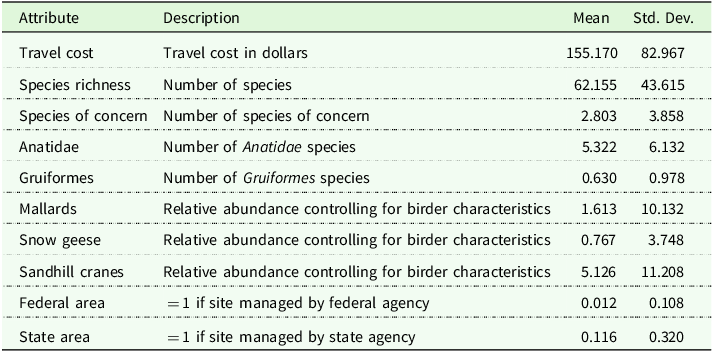
The RUM model indicates that birders derive utility from sandhill cranes and species richness, but not from the abundance of other species or the presence of endangered species (Table 2). Column (1) presents the preference parameters in our benchmark specification. The coefficient on number of species is positive (p < 0.001), implying that a person is more likely to visit a site with a greater variety of birds. The coefficient on Anatidae is not significantly different from zero, suggesting there may be no premium associated with the presence of ducks and geese. This implies that the presence of an additional Anatidae species contributes about as much to utility as another species, on average. The positive coefficient on Gruiformes (p = 0.023) means that birders put a premium on sites that attract cranes. The negative coefficient on species of concern (p < 0.001) may appear counterintuitive, as one might expect that birders would prefer rare species. However, this estimate could reflect the challenge of observing rare birds; sites with threatened or endangered species can have poor visibility, restricted access, or require more specialized knowledge and patience to successfully spot birds. The average birder may prefer sites with more reliable and accessible viewing experiences. None of the abundance coefficients – for mallards, snow geese, or sandhill cranes – are significantly different from zero.
RUM model parameters

Travel cost standard error calculated using a parametric bootstrap around the contraction mapping; other standard errors calculated using regression and clustered on counties in parentheses. *p < 0.10, **p < 0.05, ***p < 0.01.
The other columns add different varieties of fixed effects to control for potential confounders. Column (2) includes site fixed effects to control for time-invariant site characteristics. Otherwise, no comprehensive database exists for attributes such as parking access, entry fees, trail length, and site-specific conservation measures. Including site fixed effects controls for these potential confounders and shifts identification to within-site temporal variation. Most coefficients maintain their sign and significance level, except for crane abundance, which turns significantly positive (p = 0.013). Controlling for omitted characteristics produces estimates that indicate birders prefer greater crane populations on the margin. Converting this preference to monetary terms by dividing the crane parameter by the travel cost parameter yields a WTP of $0.09 for a one-unit increase in relative abundance, or $0.98 for an increase of one standard deviation (roughly tripling abundance at the mean).
Column (3) replaces the site fixed effects with county-by-season effects, allowing us to identify preferences from variation in richness and abundance across sites within the same county and season. The estimates remain largely similar to those in column (2), providing additional evidence that birders prefer sites with cranes. Converted to monetary terms, the crane preference equates to a WTP of $0.08 for a one-unit increase in relative abundance or $0.90 for a one standard deviation increase.
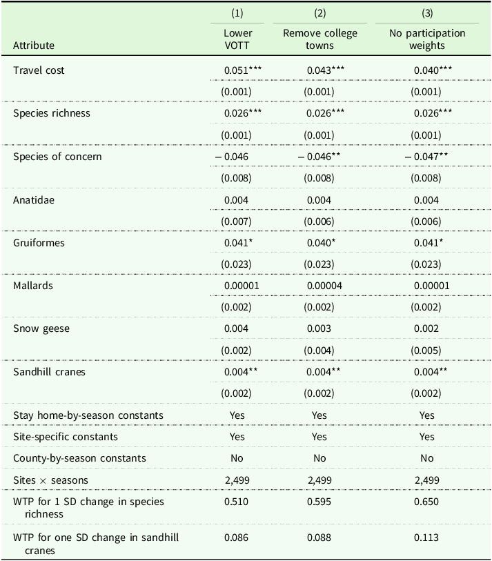
Now consider the model with site fixed effects under alternative assumptions (Table 3). One concern is that the estimates will be sensitive to VOTT, so column (1) reduces VOTT from one-half to one-third the wage rate. Only the travel cost parameter noticeably changes, implying a WTP of $0.08 for a one-standard deviation increase in crane abundance. Another concern is that eBird volunteers are disproportionately scientists and academics, which could skew birding activity toward college towns. Column (2) addresses this concern by removing sites in the same ZIP code as Indiana’s largest universities.Footnote 2 Estimates are practically unchanged. Finally, we examine sensitivity to the assumed population distribution by removing participation weights; now the modeled travel flows are based on the residential locations of the entire population rather than birders. This produces a lower travel cost parameter and a WTP of $0.11 for a one-unit increase in crane abundance. Not shown but available upon request are several additional regressions that show results are largely insensitive to controlling for the local abundance of other species; only the effect of cranes comes out significantly positive in these regressions. The results are also insensitive to re-scaling the estimates using the travel cost parameter from fall 2022 rather than fall 2021.
Sensitivity analysis of RUM model assumptions

Travel cost standard error calculated using a parametric bootstrap around the contraction mapping; other standard errors calculated using regression and clustered on counties in parentheses. *p < 0.10, **p < 0.05, ***p < 0.01.
To summarize, the RUM model shows that birders prefer locations with more species and greater crane abundance after controlling for a large set of potential confounders. They reveal no preference for other types of waterbirds, which suggests that population abundance is a key driver for only some species.
The welfare effects of crane population movements
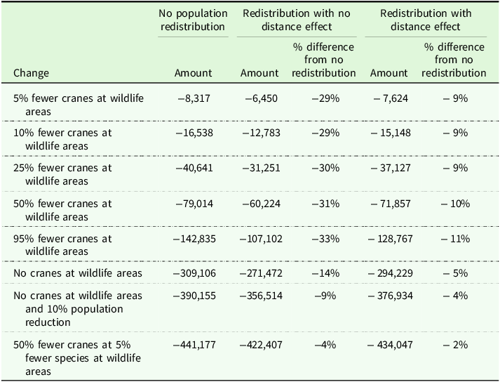
We now consider the welfare estimates from eight changes in local crane abundance (Table 4). The first five changes simulate a hypothetical crane hunt centered around state wildlife areas, which would reduce local abundance near these sites with statewide population held constant.Footnote 3 The first column considers the direct effects, without coupling the RUM and connectivity models. Birder WTP is just over $8,300 to avoid a 5% reduction in cranes, $16,500 for a 10% reduction, and $79,000 for a 50% reduction. These estimates indicate that smaller changes at state wildlife areas (which we think is a realistic representation of how local abundance would likely respond to hunting) reduce welfare by only a few thousand dollars, although losses do grow with larger changes in local abundance.
Welfare changes (in 2022 $) under alternative population models for sandhill cranes

Note: These wildlife areas include 22 sites.
The second column shows the estimates when we account for spatial connectivity using Equation (6) with the distance effect turned off ( $\mu = 0$
). This redistributes the reduction based purely on abundance at other sites. Although the biological loss and gain exactly offset each other, nevertheless there are welfare consequences: a loss of $6,500 for a 5% reduction, $12,800 for a 10% reduction, and $60,200 for a 50% reduction. Accounting for connectivity produces smaller estimates than the direct effects alone.
$\mu = 0$
). This redistributes the reduction based purely on abundance at other sites. Although the biological loss and gain exactly offset each other, nevertheless there are welfare consequences: a loss of $6,500 for a 5% reduction, $12,800 for a 10% reduction, and $60,200 for a 50% reduction. Accounting for connectivity produces smaller estimates than the direct effects alone.
The third column presents the estimates using Equation (6) with the distance effect turned on ( $\mu = 1$
). Now the economic losses are $7,600 for a 5% reduction, $15,100 for a 10% reduction, and $71,900 for a 50% reduction. This version of the connectivity model implies that re-sorting cranes are willing to trade off distance for habitat quality, some moving to nearby sites with minimal prior crane abundance, which tend to attract fewer birders. Losses are therefore larger than those in the second column because cranes are redistributing to less desirable sites for bird watchers.
$\mu = 1$
). Now the economic losses are $7,600 for a 5% reduction, $15,100 for a 10% reduction, and $71,900 for a 50% reduction. This version of the connectivity model implies that re-sorting cranes are willing to trade off distance for habitat quality, some moving to nearby sites with minimal prior crane abundance, which tend to attract fewer birders. Losses are therefore larger than those in the second column because cranes are redistributing to less desirable sites for bird watchers.
The final three scenarios in Table 5 simulate more substantial changes in crane abundance as well as species richness. The first completely eliminates cranes, which affects utility both through a reduction in local abundance and the removal of a species. This produces a welfare loss of $271,000 to $309,000, depending on how we model connectivity. One concern is that a significant redistribution of cranes could reduce survival rates, lowering the statewide population. The next scenario investigates this concern by pairing local elimination with a 10% population decline. This produces a larger welfare loss of $357,000 to $390,000. Finally, recognizing that crane hunting could disturb other wildlife through habitat disruption, the last scenario combines a 50% crane reduction with a 5% decline in species richness at state wildlife areas. This produces the largest welfare loss across all scenarios: $422,000 to $441,000.
Discussion
Ignoring connectivity in wildlife viewing produces upwardly biased losses following targeted reductions in local abundance. Losses in our application are lower once we account for spatial connectivity. The bias ranges from 9% for 5% fewer cranes at state wildlife areas to 34% for a 95% reduction, depending on how we model connectivity.
This bias is consistent with Newbold and Massey (Reference Newbold and Massey2010), who find that failing to structurally model spatially and temporally endogenous wildlife leads to overestimates of willingness to pay to avoid reductions in habitat quality. Their simulations show values ignoring spillovers can be several times larger than the true value, depending on the sophistication of the connectivity model.
Our analysis shows that the bias from ignoring connectivity can be small if wildlife redistribute with distance-dependent behavior. For example, 5% fewer cranes at state wildlife areas produces a loss of $8,300 ignoring connectivity effects, $7,600 with a distance effect and $6,500 without it. Our empirical analysis does not identify the effect of distance, so the actual welfare loss could be closer to or further from $8,300. If nearby sites are better substitutes than distant ones, omitting distance from the connectivity model will underestimate the welfare loss, providing a lower bound.
Overlooking wildlife connectivity may not always lead to upwardly biased welfare estimates. One potential criticism is that the analysis oversimplifies connectivity while failing to account for population dynamics. Habitat loss can impact local abundance as well as overall population. If changes at targeted sites lower abundance at other sites, for example because of critical habitat loss, then conventional estimates could be biased downward. This is why we considered a scenario with a 10% statewide population reduction, although this is a static assumption rather than an endogenously determined outcome. A more sophisticated approach would integrate species-level responses to habitat changes and metapopulation dynamics. Consequently, the true welfare impacts of crane hunting could differ from our estimates, particularly over longer time horizons as the population adapts to new ecological conditions. The direction and magnitude of this bias remain uncertain – the crane population could experience a severe decline if critical habitat thresholds are crossed, or alternatively, their adaptability leads to a complete recovery. Indeed, sandhill crane populations have demonstrated resilience, rebounding significantly from 20th-century lows (Lacy et al. Reference Lacy, Barzen, Moore and Norris2015). This resilience suggests that the welfare losses reported here could attenuate over time because the population will recover.
Another potential criticism is that our application finds greatly reducing the population of an important species at state wildlife areas impacts welfare only up to several hundred thousand dollars per year – an amount that may seem modest. However, this estimate needs to be contextualized. First, state wildlife areas host twice as many species as the average site and species richness is an important driver of visitation. Crane abundance may matter to birders, but cranes are just one among many species and thus their removal tends to affect welfare incrementally rather than substantially. Second, state wildlife areas are remote, rural locations which limits their accessibility, accounting for less than 1% of eBird trips in Indiana. Of these, the RUM model indicates that only a fraction would shift to other sites following a major population decline.Footnote 4 Third, the welfare calculations capture only use values from viewing activities, which is just one component of cranes’ total economic value. There will of course be non-use values for species that hold cultural significance like cranes.Footnote 5
Species richness is a valuable site attribute, and the presence of cranes is more valuable than large increases in local abundance. WTP more than doubles from $107,000–$143,000 to avoid a 95% reduction to $271,000–$309,000 to avoid complete elimination. This disproportionate jump, driven by a shift from crane presence to absence, highlights the discrete value birders place on species presence. Losses also increase substantially when other species are absent from a site. When a 50% crane reduction in our application is accompanied by a 5% decline in overall species richness, WTP increases from $60,000–$79,000 to $422,000–$441,000.Footnote 6
How do the estimates in our application line up with prior research? We can compare values for species richness and site access, both of which can be found in the literature. The richness and travel cost parameters in our model indicate that WTP is $0.60 per trip for an additional species and $22.96 per trip for site access. Using eBird data from Alberta, Jayalath et al. (Reference Jayalath, Lloyd-Smith and Becker2023) estimate WTP at CAN$0.68 (US$0.64 in 2022 dollars) per trip for an additional species and CAN$36.30 (US$34.10 in 2022 dollars) per trip for site access. Adjusted for inflation, Aiken (Reference Aiken2009) estimates the value of wildlife viewing in Indiana is $40.23 per trip, while Huber and Sexton (Reference Huber and Sexton2019) find WTP is $80.15 per day for crane viewing sites in New Mexico. Melstrom et al. (Reference Melstrom, Nielsen and Reeling2024) report WTP is $0.58 per trip for an additional species and $27.67 per day for three wildlife areas in Indiana. Our WTP estimates for species richness align closely with other studies, while our estimate of site access falls on the low end of previous estimates.
We acknowledge that wildlife can respond to disturbances in different ways, including behavioral responses (like avoidance, emigration, and changes in the timing or amount of activity) and demographic responses (changes in mortality, recruitment) (Sergio et al. Reference Sergio, Blas and Hiraldo2018). We model birdwatcher utility as a function of abundance at a particular site; hence, the relevant responses are those that manifest as changes in the number of birds or mix of species seen. Our modeling framework can flexibly accommodate many different response types, depending on the type of wildlife and disturbance being modeled. For example, wildlife may adjust to seasonal disturbances (like hunting) by altering the timing of migration through a site. We could simulate this in a manner very similar to the population shocks we describe here (reducing abundance at hunting sites during the season, with sorting to determine emigration to alternative sites). Wildlife populations may also adjust via maladaptive site fidelity – i.e., by failing to relocate and instead reducing in number following a disturbance. This is akin to the shocks prior work simulates (a reduction in abundance at a specific site without compensatory increases in spatially connected sites).
Before concluding, we should note that using eBird data in our application to measure visitation patterns comes with limitations. First, eBird users represent a subset of birders who may be more dedicated and avid than the average birdwatcher. This could bias the sample toward more distant, non-local trips if eBird users tend to travel farther (Cameron and Kolstoe Reference Cameron and Kolstoe2022). Second, eBird checklists may not accurately reflect overall visitation since users might preferentially submit observations from locations with charismatic species while underreporting visits to sites with common birds. The temporal patterns of data submission could also be skewed, as users may be more likely to submit checklists during peak migration periods or organized events like the Christmas Bird Count. Furthermore, variations in cell phone coverage and internet access could affect submission rates, potentially underrepresenting more remote locations. Finally, there may be cultural and regional differences in eBird adoption rates that challenge extrapolating visitation patterns from eBird to all birders, particularly in areas where the platform has lower participation rates or where different viewing behaviors prevail.
Conclusion
This study showed that nonmarket valuation of wildlife viewing is sensitive to ecological connectivity and wildlife mobility. When disturbances or management changes occur at one site, they can alter wildlife distributions and viewing opportunities elsewhere. We examined the potential for valuation bias by pairing models of recreation demand and wildlife connectivity.
Our results showed that conventional approaches that ignore connectivity overestimate welfare losses. The bias was as high as 34% in our empirical application, which indicates that in some contexts the additional complexity of modeling wildlife mobility could yield large improvements in valuation accuracy. It also indicates that in situ redistribution to alternative sites only partially mitigates the welfare effect of a disturbance at one site.
Overlooking wildlife connectivity does not necessarily produce upwardly biased welfare estimates. Our research focused on spatial connectivity and did not consider population dynamics, which is another source of bias. Habitat loss at one site could cause a decline in local abundance at connected sites. Conventional estimates in this case could be biased downward. It is also possible that wildlife redistribution and population dynamics could lead to offsetting effects at connected sites.
Our application measured site preferences using visitation, species richness, and abundance data from eBird. Indiana birders prefer sites characterized by greater richness and more abundant sandhill crane populations. Birders were willing to pay $0.60 per trip for an additional species and $0.98 per trip for a one-standard-deviation increase in crane abundance. Policy simulations showed that displacing 50% of cranes from state wildlife areas would generate economic losses of $60,000 to $79,000 per year, depending on how displaced birds redistribute to alternative sites. This range jumps to $422,000 to $441,000 if the loss is accompanied by a 5% reduction in the number of species. These estimates underscore that both presence-absence and abundance are economically meaningful drivers of wildlife values and that presence-absence effects are particularly important.
Research that measures wildlife values and accounts for spatial connectivity is becoming more important as wildlife management incorporates economic considerations. Future research could explore other species and conservation policies. Additional research comparing the preferences of eBird users to other recreationists would also be valuable. Although our application integrated macro-level data from a visitor survey in one part of the study region, integrating microdata from a representative household survey could lead to more precise estimates while shedding additional light on the generalizability of eBird users.
Data availability statement
Data and code are available from the corresponding author.
Funding statement
This project was funded by a Wildlife Restoration program grant W-49-R-05 in cooperation with the Indiana Department of Natural Resources, Division of Fish & Wildlife, and the US Fish & Wildlife Service. The authors would like to thank Adam Phelps for helpful comments and Caitlyn Smith for research assistance.
Competing interests
Melstrom, Edmonds, and Reeling declare none.


 Open access