


1. Introduction
As a granular material constituted of an interconnected network of ice grains, snow has a complex mechanical behaviour influenced both by the material properties of ice and by its intrinsic microstructure. As a homogeneous material, ice can show both brittle and ductile behaviour, depending on the external conditions as strain rate for instance (Schulson, Reference Schulson1990). It also exhibits temperature-dependant creep behaviour (Barnes and others, Reference Barnes, Tabor and Walker1971). From a microscopic perspective, snow exhibits diverse microstructures initially dictated by the meteorological conditions at snowfall but evolving over time under the influence of the environmental constraints. This so-called snow metamorphism is mostly driven by the temperature and its gradient within the snow layer. Under specific climatic conditions, snow metamorphism leads to the transformation of snowflakes into bonded spherical ice grains (Fierz, Reference Fierz2009; Calonne and others, Reference Calonne, Flin, Geindreau, Lesaffre and du Roscoat2014) which normally goes along with a snow densification (Kojima, Reference Kojima1967).
Modelling the mechanical behaviour of snow is of great interest in various fields, from avalanche prediction and mitigation (Nicot, Reference Nicot2004; Gaume and others, Reference Gaume, Chambon, Eckert, Naaim and Schweizer2015), winter sports equipment (Fauve and others, Reference Fauve, Rhyner, Lüthi, Schneebeli and Lehning2008), to snow tire design (Shoop and others, Reference Shoop, Kestler and Haehnel2006; Lee, Reference Lee2013; Hjort and others, Reference Hjort, Eriksson and Bruzelius2017). Two kinds of approaches are widely adopted for snow modelling, namely continuum-based and particle-based methods. Particle-based methods have the advantage of explicitly accounting for the characteristics of snow microstructure. They are based on an individual representation of grains, mostly through the discrete element method (DEM) (Cundall and Strack, Reference Cundall and Strack1979; Radjai and others, Reference Radjai, Wolf, Jean and Moreau1998; Luding, Reference Luding2008; Smilauer, Reference Smilauer2010). DEM has already been used for snow by modelling the ice grains as discrete particles connected by ice bonds (Johnson and Hopkins, Reference Johnson and Hopkins2005; Mede and others, Reference Mede, Chambon, Hagenmuller and Nicot2018; Mulak and Gaume, Reference Mulak and Gaume2019; Willibald and others, Reference Willibald, Scheuber, Löwe, Dual and Schneebeli2019; Bobillier and others, Reference Bobillier, Bergfeld, Dual, Gaume, van Herwijnen and Schweizer2021; Kabore and others, Reference Kabore, Peters, Michael and Nicot2021; Peters and others, Reference Peters, Kabore, Michael and Nicot2021) or to represent snow elements (Gaume and others, Reference Gaume, van Herwijnen, Chambon, Birkeland and Schweizer2015). In return for taking effective account of the effect of the microstructure, DEM is computationally costly, which limits its ability to model large scale systems. As an alternative to discrete numerical methods, continuum-based approaches of snow include the finite element method (Meschke and others, Reference Meschke, Liu and Mang1996; Podolskiy and others, Reference Podolskiy, Chambon, Naaim and Gaume2013; Fourteau and others, Reference Fourteau, Freitag, Malinen and Löwe2024), the finite difference method (Dent and Lang, Reference Dent and Lang1980), the material point method (Gaume and others, Reference Gaume, Gast, Teran, van Herwijnen and Jiang2018, Reference Gaume, van Herwijnen, Gast, Teran and Jiang2019; Trottet, Reference Trottet2022) and the smooth particles hydrodynamics (El-Sayegh and El-Gindy, Reference El-Sayegh and El-Gindy2019) among others. In these methods, snow is modelled as a continuous medium and its material behaviour is accounted for by a constitutive relation. For example, a Drucker-Prager (Haehnel and Shoop, Reference Haehnel and Shoop2004; Lee, Reference Lee2009; Gaume and others, Reference Gaume, Chambon, Naaim, Eckert, Bonelli, Dascalu and Nicot2011; Blatny and others, Reference Blatny, Löwe and Gaume2023) or a modified Cam-Clay (Gaume and others, Reference Gaume, Gast, Teran, van Herwijnen and Jiang2018; Guillet and others, Reference Guillet, Blatny, Trottet, Steffen and Gaume2023) constitutive material laws are widely used in the field of snow avalanche modelling. Such approaches are usually significantly less time-consuming than DEM, meaning that they can address large scale systems. However, the constitutive relations implemented are generally phenomenological and therefore do not explicitly account for the snow microstructure, which makes them harder to calibrate. However, recent works have highlighted the importance of incorporating snow microstructure into constitutive models to more accurately capture its mechanical behaviour (Blatny and others, Reference Blatny, Löwe, Wang and Gaume2021, Reference Blatny, Löwe and Gaume2023).
In this paper, we propose a continuum approach based on a constitutive material model that incorporates explicitly the discrete microstructure of snow, thus combining the advantages of both modelling strategies. To this end, the 3-D H-model (Nicot and Darve, Reference Nicot and Darve2011; Xiong and others, Reference Xiong, Nicot and Yin2017) is extended to snow, considered as an assembly of spherical ice particles connected by ice bonds. This model was originally introduced for soil modelling in dry (Wautier, Reference Wautier2021) and partially saturated conditions (Xiong, Reference Xiong2021). The ability of the H-model to be used at large scale has been demonstrated by Xiong and others (Reference Xiong, Yin and Nicot2019), where the 3-D H-model is used to model geotechnical problems. In this approach, a granular material is described as a distribution of mesostructures formed by a few grains. The collection of these mesostructures (denoted H-cells in the following) in various configurations provides a statistical description of the microstructure. From the individual mechanical response of each mesostructure, the material constitutive relation can be formulated in a continuum framework by statistical homogenization. In the hereafter presented extension of the 3-D H-model, the particles forming the H-cells represent ice grains with an interparticle contact law specifically suited to ice. The latter was developed to capture the ice bond evolution as well as the ice grain contact and is partly based on a previous work (Kabore and others, Reference Kabore, Peters, Michael and Nicot2021). As many engineering applications (vehicles moving on snow, winter sports, …) imply short-term time scales and fast loading, only the brittle behaviour of ice will be considered in the following. Since density is one of the most important parameters in snow behaviour, special attention is brought to the relationship between the geometry of the mesostructures in the H-model and the macroscopic density. The influence of the aging of snow before the mechanical loading and its impact on the calibration of the numerical parameter are also investigated. Finally, the capacity of the model to account for varying conditions such as the temperature and the loading rate is demonstrated.
2. Multi-scale model for snow
The H-model was initially developed for granular soils, first in two dimensions (Nicot and Darve, Reference Nicot and Darve2011; Veylon and others, Reference Veylon, Nicot, Zhu and Darve2018) before being extended to three dimensions (Xiong and others, Reference Xiong, Nicot and Yin2017). It has been progressively extended to capture additional physical phenomena, such as the existence of capillary forces in unsaturated soils (Wautier, Reference Wautier2021; Xiong, Reference Xiong2021), or erosion by suffusion (Ma and others, Reference Ma, Wautier and Nicot2022). Here, further extension of the 3-D H-model to snow modelling relies on implementing a specific customized contact law for ice bonds, restricting the scope of the study to fast loading conditions (strain rate above  ${10^{ - 4}}{{\text{s}}^{ - 1}}{ }$), so that the ice behaviour can be assumed to be exclusively brittle (Schulson, Reference Schulson1990).
2.1. A multi-scale constitutive model for granular materials: the 3-D H-model
Contrary to phenomenological approaches, multi-scale models introduce a statistical homogenization process, which consists in inferring the mechanical behaviour of a given material from the constitutive properties taking place at a smaller microscopic scale (Wautier, Reference Wautier2021). More precisely, the material constitutive law is obtained from the weighted averaged behaviours of several mesostructures, which are each constituted by a set of grains. First conceptualized by Satake (Reference Satake1992) and later explored by Kruyt and Rothenburg (Reference Kruyt and Rothenburg1996), grain loops are an example of such mesostructures in a 2-D granular assembly. In principle, these loops enable a geometrical description through a particle graph paving the space and have been shown to be a powerful tool to explain the behaviour of granular materials based on local physics. Namely, it has been observed that grain loops containing more than six grains within a granular material can serve as a meaningful descriptor for the material scale behaviour (Zhu and others, Reference Zhu, Veylon, Nicot and Darve2016, Reference Zhu, Nicot and Darve2016a, Reference Zhu, Nicot and Darve2016b; Liu and others, Reference Liu, Nicot and Zhou2018). These results support the physical suitability of the H-model in which the microstructure is described as a collection of either hexagonal grain assemblies in the 2-D H-model (Nicot and Darve, Reference Nicot and Darve2011) or bi-hexagonal grain assemblies in the 3-D H-model (Xiong and others, Reference Xiong, Nicot and Yin2017).
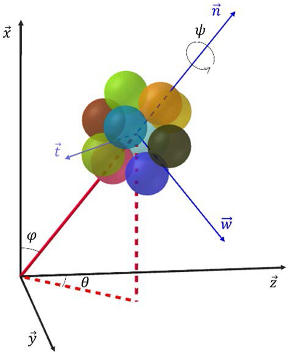
The tridimensional bi-hexagonal mesostructure is formed of two perpendicular hexagons as represented in Fig. 1. Each H-cell has an orientation in space, characterized by the three Euler angles  $\varphi $, $\theta $ and $\psi $ with respect to the global reference frame. The distribution of this orientation $\omega \left( {\theta ,\varphi ,\psi } \right){ }$ describes the initial anisotropy of the microstructure. The two hexagons of the mesostructure are supposed to remain in orthogonal planes over any loading. The planar geometry of the two hexagons is shown in Fig. 2. By adopting symmetry assumptions in the cell geometry, each hexagon can be parameterized by only two intergranular distances (
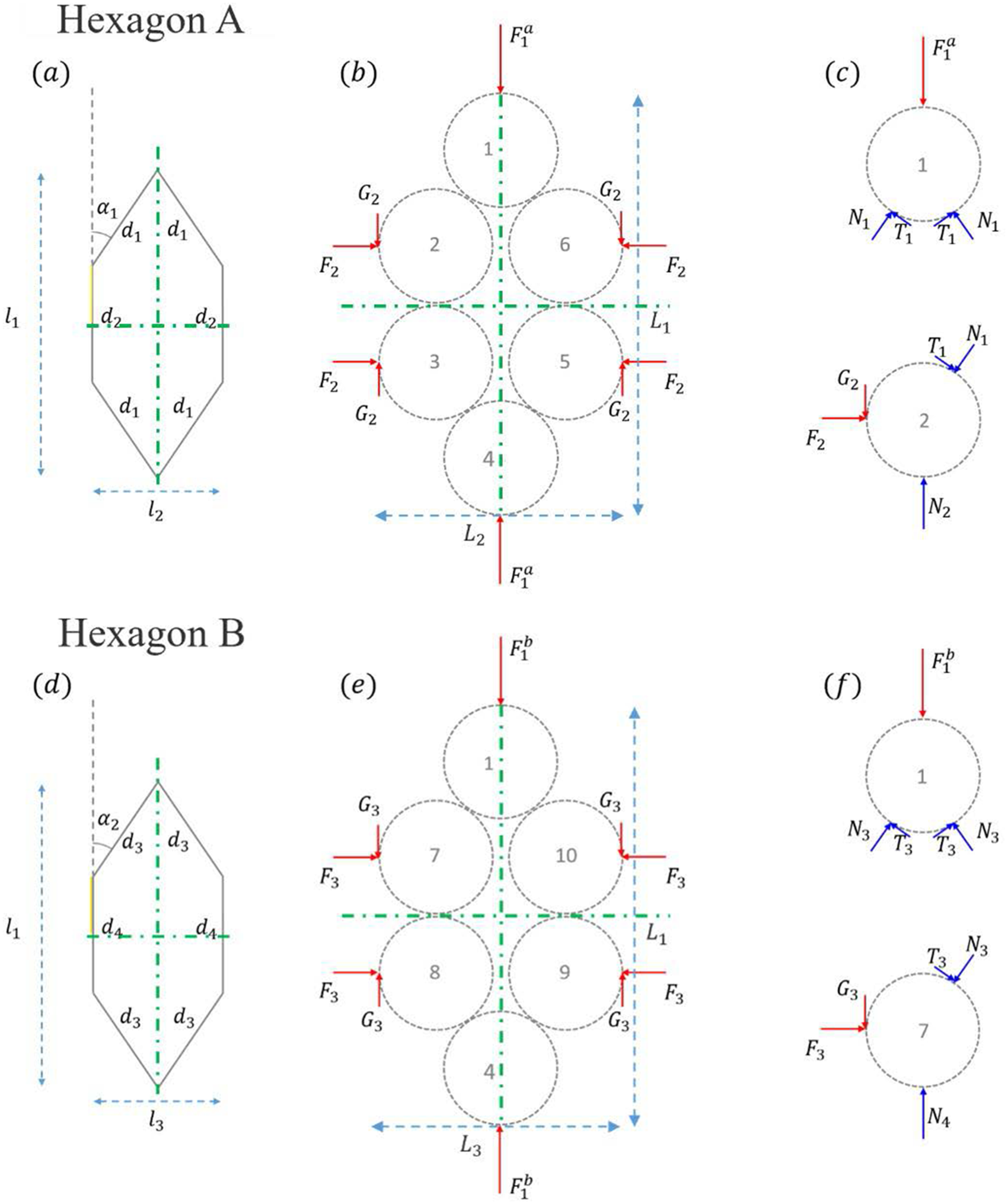
 ${d_1}$ and ${d_2}$ in hexagon A, and ${d_3}$ and ${d_4}$ in hexagon B) and an opening angle ( ${\alpha _1}$ in hexagon A and ${\alpha _2}$ in hexagon B). The symmetries in the cell allow to consider only four different contact points, between grains 1–2, 2–3, 1–7 and 7–8. To maintain the overall symmetry assumption in the cell geometry, equality is also imposed between the various forces within the cell: ${F_{\text{i}}}$ and ${G_{\text{i}}}$, representing the normal and tangential external forces in the three directions of the space, and ${N_{\text{i}}}$ and ${T_{\text{i}}}$, representing the normal and tangential contact forces at the four different contact points between the grains, as described in Fig. 2. The external vertical force on grain 1 can be decomposed into two terms $F_1^a$ and $F_1^b$, which respectively insure the equilibrium of hexagons A and B.
3-D bi-hexagonal mesostructure in the global reference frame with the definition of the Euler angles.
Schematic representation of the two hexagonal grain configurations constituting the 3-D H-cell showing: (a, d) geometry of the hexagons, (b, e) external forces on the hexagons and (c, f) equilibrium of forces on the grains. The dashed-dotted green lines represent the symmetry axis in the considered plane.
Depending on the loading of the cells, some contacts between grains can appear or be lost. Appendices C and D describe these potential cases in detail.
The overall homogenization scheme used for the H-model, as summarized in Fig. 3, allows connecting continuum/macroscale and particle/microscale descriptions of the material. An incremental constitutive relation linking the global incremental strain tensor  ${{\delta }}\underline {\underline {\boldsymbol{\varepsilon }} } $ to the global incremental stress ${{\delta }}\underline {\underline {\boldsymbol{\sigma }} } $ is thus implicitly derived. In the following, we briefly review the main steps of this homogenization scheme.
Schematic representation of overall sequence of the 3-D H-model methodology.

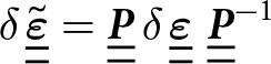
The model assumes strain homogeneity such that the same macroscopic strain is applied in all H-cells. Consequently, the local incremental strain tensor  ${{\delta }}\underline {\underline {\widetilde {\boldsymbol{\varepsilon }}} } $ in each H-cell is expressed in the local frame as
 \begin{equation}{{\delta }}\,\underline {\underline {\widetilde {\boldsymbol{\varepsilon }}} } = \underline {\underline {\boldsymbol{P}} }\,{{\delta }}\,\underline {\underline {\boldsymbol{\varepsilon }} } \,\,{ }{\underline {\underline {\boldsymbol{P}} } ^{ - 1}}\end{equation}
 with  $\underline {P}$ being the rotation matrix between the global and local frames:
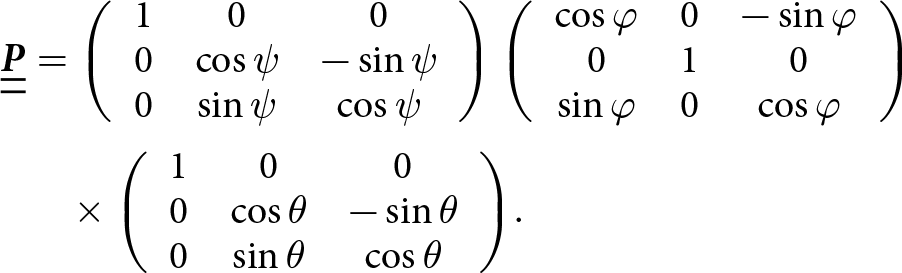 \begin{align}\underline {\underline {\boldsymbol{P}} }& = \left( {\begin{array}{*{20}{c}}
1&0&0 \\
0&{\cos \psi }&{ - \sin \psi } \\
0&{\sin \psi }&{\cos \psi }
\end{array}} \right)\left( {\begin{array}{*{20}{c}}
{\cos \varphi }&0&{ - \sin \varphi } \\
0&1&0 \\
{\sin \varphi }&0&{\cos \varphi }
\end{array}} \right)\nonumber\\ &\quad{}\times\left( {\begin{array}{*{20}{c}}
1&0&0 \\
0&{\cos \theta }&{ - \sin \theta } \\
0&{\sin \theta }&{\cos \theta }
\end{array}} \right)\!.\end{align}
\begin{align}\underline {\underline {\boldsymbol{P}} }& = \left( {\begin{array}{*{20}{c}}
1&0&0 \\
0&{\cos \psi }&{ - \sin \psi } \\
0&{\sin \psi }&{\cos \psi }
\end{array}} \right)\left( {\begin{array}{*{20}{c}}
{\cos \varphi }&0&{ - \sin \varphi } \\
0&1&0 \\
{\sin \varphi }&0&{\cos \varphi }
\end{array}} \right)\nonumber\\ &\quad{}\times\left( {\begin{array}{*{20}{c}}
1&0&0 \\
0&{\cos \theta }&{ - \sin \theta } \\
0&{\sin \theta }&{\cos \theta }
\end{array}} \right)\!.\end{align} The changes in the H-cell lengths  ${{\delta }}{L_{\text{i}}}$ can be deduced from the diagonal coefficients of the local incremental strain tensor and the external length of the H-cell ${L_{\text{i}}}$, as defined in Fig. 2:
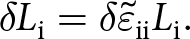 \begin{equation}{{\delta }}{L_{\text{i}}} = {{\delta }}{\tilde \varepsilon _{{\text{ii}}}}{L_{\text{i}}}.\end{equation}
The evolution of the H-cell geometry depends directly on the variations of the H-cell lengths and on the force balance applied to the mesostructure. The geometrical compatibility equations read:
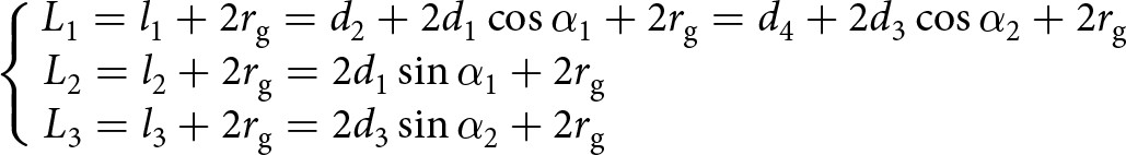 \begin{align}\left\{ \!\!{\begin{array}{*{20}{c}}
{{L_1} = {l_1} + 2{r_{\text{g}}} = {d_2} + 2{d_1}\cos {\alpha _1} + 2{r_{\text{g}}} = {d_4} + 2{d_3}\cos {\alpha _2} + 2{r_{\text{g}}}} \\
\!\!\!\!\!\!\!\!\!\!\!\!\!\!\!\!\!\!\!\!\!\!\!\!\!\!\!\!\!\!\!\!\!\!\!\!\!\!\!\!\!\!\!\!\!\!\!\!\!\!\!\!\!\!\!\!\!\!\!\!\!\!\!\!\!\!\!\!\!\!\!\!{{L_2} = {l_2} + 2{r_{\text{g}}} = 2{d_1}\sin {\alpha _1} + 2{r_{\text{g}}}{ }} \\
\!\!\!\!\!\!\!\!\!\!\!\!\!\!\!\!\!\!\!\!\!\!\!\!\!\!\!\!\!\!\!\!\!\!\!\!\!\!\!\!\!\!\!\!\!\!\!\!\!\!\!\!\!\!\!\!\!\!\!\!\!\!\!\!\!\!\!\!\!\!\!\!{{L_3} = {l_3} + 2{r_{\text{g}}} = 2{d_3}\sin {\alpha _2} + 2{r_{\text{g}}}{ }}
\end{array}} \right.\nonumber\\ \end{align}
\begin{align}\left\{ \!\!{\begin{array}{*{20}{c}}
{{L_1} = {l_1} + 2{r_{\text{g}}} = {d_2} + 2{d_1}\cos {\alpha _1} + 2{r_{\text{g}}} = {d_4} + 2{d_3}\cos {\alpha _2} + 2{r_{\text{g}}}} \\
\!\!\!\!\!\!\!\!\!\!\!\!\!\!\!\!\!\!\!\!\!\!\!\!\!\!\!\!\!\!\!\!\!\!\!\!\!\!\!\!\!\!\!\!\!\!\!\!\!\!\!\!\!\!\!\!\!\!\!\!\!\!\!\!\!\!\!\!\!\!\!\!{{L_2} = {l_2} + 2{r_{\text{g}}} = 2{d_1}\sin {\alpha _1} + 2{r_{\text{g}}}{ }} \\
\!\!\!\!\!\!\!\!\!\!\!\!\!\!\!\!\!\!\!\!\!\!\!\!\!\!\!\!\!\!\!\!\!\!\!\!\!\!\!\!\!\!\!\!\!\!\!\!\!\!\!\!\!\!\!\!\!\!\!\!\!\!\!\!\!\!\!\!\!\!\!\!{{L_3} = {l_3} + 2{r_{\text{g}}} = 2{d_3}\sin {\alpha _2} + 2{r_{\text{g}}}{ }}
\end{array}} \right.\nonumber\\ \end{align} with  ${L_{\text{i}}}$ the lengths of the smallest peripheral parallelepiped volume, ${l_{\text{i}}}$ the lengths of the hexagons defined by the centres of the grains and ${r_{\text{g}}}$ the grain radius.
Differential variation of Eqn (4) provides three equations relating the variations of the H-cell lengths  ${{\delta }}{L_{\text{i}}}$ to the variations of both the intergranular distances ${{\delta }}{d_{\text{i}}}$ and the opening angles ${{\delta }}{\alpha _{\text{i}}}:$
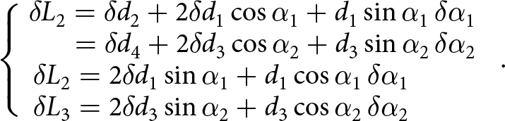 \begin{equation}\left\{\kern-8pt\begin{array}{c}\;\;\delta L_2=\delta d_2+2\delta d_1\cos\alpha_1+d_1\sin\alpha_1\,\delta\alpha_1\\\;\;\;\;\;\;\;\;=\delta d_4+2\delta d_3\cos\alpha_2+d_3\sin\alpha_2\,\delta\alpha_2\\\delta L_2=2\delta d_1\sin\alpha_1+d_1\cos\alpha_1\,\delta\alpha_1\;\;\;\;\;\;\;\\\delta L_3=2\delta d_3\sin\alpha_2+d_3\cos\alpha_2\,\delta\alpha_2\;\;\;\;\;\;\;\end{array}\right..\!\\\end{equation}
Considering the balance of forces and momentum for the grains 2 and 7 provides:
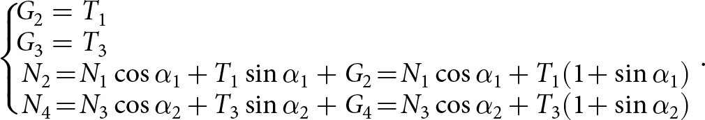 \begin{align}\left\{ \!\!{\begin{array}{c}
\!\!\!\!\!\!\!\!\!\!\!\!\!\!\!\!\!\!\!\!\!\!\!\!\!\!\!\!\!\!\!\!\!\!\!\!\!\!\!\!\!\!\!\!\!\!\!\!\!\!\!\!\!\!\!\!\!\!\!\!\!\!\!\!\!\!\!\!\!\!\!\!\!\!\!\!\!\!\!\!\!\!\!\!\!\!\!\!\!\!\!\!\!\!\!\!\!\!\!\!\!\!\!\!\!\!\!\!\!\!\!\!\!\!\!\!\!\!\!\!\!\!\!\!\!\!\!\!{{G_2} = {T_1}\,} \\
\!\!\!\!\!\!\!\!\!\!\!\!\!\!\!\!\!\!\!\!\!\!\!\!\!\!\!\!\!\!\!\!\!\!\!\!\!\!\!\!\!\!\!\!\!\!\!\!\!\!\!\!\!\!\!\!\!\!\!\!\!\!\!\!\!\!\!\!\!\!\!\!\!\!\!\!\!\!\!\!\!\!\!\!\!\!\!\!\!\!\!\!\!\!\!\!\!\!\!\!\!\!\!\!\!\!\!\!\!\!\!\!\!\!\!\!\!\!\!\!\!\!\!\!\!\!\!\!{{G_3} = {T_3}\,} \\
\!{{N_2} \!=\! {N_1}\cos {\alpha _1} \,{+}\, {T_1}\sin {\alpha _1} + {G_2} \!=\! {N_1}\cos {\alpha _1} \,{+}\, {T_1}( {1 \!+ \sin {\alpha _1}} )} \\
\!{{N_4} \!=\! {N_3}\cos {\alpha _2} \,{+}\, {T_3}\sin {\alpha _2} + {G_4} \!=\! {N_3}\cos {\alpha _2} \,{+}\, {T_3}( {1 \!+ \sin {\alpha _2}} )}
\end{array}} \right.\!\!\!.\!\!\!\nonumber\\ \end{align}
\begin{align}\left\{ \!\!{\begin{array}{c}
\!\!\!\!\!\!\!\!\!\!\!\!\!\!\!\!\!\!\!\!\!\!\!\!\!\!\!\!\!\!\!\!\!\!\!\!\!\!\!\!\!\!\!\!\!\!\!\!\!\!\!\!\!\!\!\!\!\!\!\!\!\!\!\!\!\!\!\!\!\!\!\!\!\!\!\!\!\!\!\!\!\!\!\!\!\!\!\!\!\!\!\!\!\!\!\!\!\!\!\!\!\!\!\!\!\!\!\!\!\!\!\!\!\!\!\!\!\!\!\!\!\!\!\!\!\!\!\!{{G_2} = {T_1}\,} \\
\!\!\!\!\!\!\!\!\!\!\!\!\!\!\!\!\!\!\!\!\!\!\!\!\!\!\!\!\!\!\!\!\!\!\!\!\!\!\!\!\!\!\!\!\!\!\!\!\!\!\!\!\!\!\!\!\!\!\!\!\!\!\!\!\!\!\!\!\!\!\!\!\!\!\!\!\!\!\!\!\!\!\!\!\!\!\!\!\!\!\!\!\!\!\!\!\!\!\!\!\!\!\!\!\!\!\!\!\!\!\!\!\!\!\!\!\!\!\!\!\!\!\!\!\!\!\!\!{{G_3} = {T_3}\,} \\
\!{{N_2} \!=\! {N_1}\cos {\alpha _1} \,{+}\, {T_1}\sin {\alpha _1} + {G_2} \!=\! {N_1}\cos {\alpha _1} \,{+}\, {T_1}( {1 \!+ \sin {\alpha _1}} )} \\
\!{{N_4} \!=\! {N_3}\cos {\alpha _2} \,{+}\, {T_3}\sin {\alpha _2} + {G_4} \!=\! {N_3}\cos {\alpha _2} \,{+}\, {T_3}( {1 \!+ \sin {\alpha _2}} )}
\end{array}} \right.\!\!\!.\!\!\!\nonumber\\ \end{align}Differentiating these last two equilibrium equations yields:
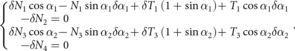 \begin{align}\left\{\kern-5pt {\begin{array}{l}
\delta {N_1}\cos {\alpha _1} \!- {N_1}\sin {\alpha _1}\delta {\alpha _1} \!+ \delta {T_1}\left( {1 + \sin {\alpha _1}} \right) \!+ {T_1}\cos {\alpha _1}\delta {\alpha _1} \\ \quad - \delta {N_2} = 0 \\
\delta {N_3}\cos {\alpha _2} \!- {N_3}\sin {\alpha _2}\delta {\alpha _2} \!+ \delta {T_3}\left( {1 + \sin {\alpha _2}} \right) \!+ {T_3}\cos {\alpha _2}\delta {\alpha _2}\\ \quad- \delta {N_4} = 0
\end{array}} \right.\!\!\!.\!\!\!\nonumber\\ \end{align}
\begin{align}\left\{\kern-5pt {\begin{array}{l}
\delta {N_1}\cos {\alpha _1} \!- {N_1}\sin {\alpha _1}\delta {\alpha _1} \!+ \delta {T_1}\left( {1 + \sin {\alpha _1}} \right) \!+ {T_1}\cos {\alpha _1}\delta {\alpha _1} \\ \quad - \delta {N_2} = 0 \\
\delta {N_3}\cos {\alpha _2} \!- {N_3}\sin {\alpha _2}\delta {\alpha _2} \!+ \delta {T_3}\left( {1 + \sin {\alpha _2}} \right) \!+ {T_3}\cos {\alpha _2}\delta {\alpha _2}\\ \quad- \delta {N_4} = 0
\end{array}} \right.\!\!\!.\!\!\!\nonumber\\ \end{align} The contact forces are related to the H-cell geometrical parameters through a contact law. In the general case of a visco-elastic contact, a generic form of the contact law at a given contact  ${\text{i}}$ reads:
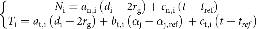 \begin{equation}\left\{\kern-5pt {\begin{array}{l}
\qquad\qquad{{N_{\text{i}}} = {a_{{\text{n}},{\text{i}}}}\left( {{d_{\text{i}}} - 2{r_{\text{g}}}} \right) + {c_{{\text{n}},{\text{i}}}}\left( {t - {t_{{\text{ref}}}}} \right)\,\,\,\,\,\,\,\,\,\,\,\,\,\,\,\,\,\,\,\,\,\,\,\,\,\,\,\,\,\,\,\,\,} \\
{{T_{\text{i}}} = {a_{{\text{t}},{\text{i}}}}\left( {{d_{\text{i}}} - 2{r_{\text{g}}}} \right) + {b_{{\text{t}},{\text{i}}}}\left( {{\alpha _{\text{j}}} - {\alpha _{{\text{j}},{\text{ref}}}}} \right)\, + {c_{{\text{t}},{\text{i}}}}\left( {t - {t_{ref}}} \right)}
\end{array}} \right.\end{equation}
\begin{equation}\left\{\kern-5pt {\begin{array}{l}
\qquad\qquad{{N_{\text{i}}} = {a_{{\text{n}},{\text{i}}}}\left( {{d_{\text{i}}} - 2{r_{\text{g}}}} \right) + {c_{{\text{n}},{\text{i}}}}\left( {t - {t_{{\text{ref}}}}} \right)\,\,\,\,\,\,\,\,\,\,\,\,\,\,\,\,\,\,\,\,\,\,\,\,\,\,\,\,\,\,\,\,\,} \\
{{T_{\text{i}}} = {a_{{\text{t}},{\text{i}}}}\left( {{d_{\text{i}}} - 2{r_{\text{g}}}} \right) + {b_{{\text{t}},{\text{i}}}}\left( {{\alpha _{\text{j}}} - {\alpha _{{\text{j}},{\text{ref}}}}} \right)\, + {c_{{\text{t}},{\text{i}}}}\left( {t - {t_{ref}}} \right)}
\end{array}} \right.\end{equation} with  ${a_{{\text{n}},{\text{i}}}}$, ${c_{{\text{n}},{\text{i}}}},$ ${a_{{\text{t}},{\text{i}}}}$, ${b_{{\text{t}},{\text{i}}}}$ and ${c_{{\text{t}},{\text{i}}}}$ being independent of the geometry. The ${a_{{\text{n}},{\text{i}}}}$ and the ${a_{{\text{t}},{\text{i}}}}$ coefficients are stiffness terms expressing the evolution of the intergranular distance in terms of the incremental contact forces (normal and tangential respectively). The coefficients ${b_{{\text{t}},{\text{i}}}}$ link the tangential contact force to the evolution of the opening angle. The coefficients ${c_{{\text{n}},{\text{i}}}}$ and ${c_{{\text{t}},{\text{i}}}}$ are viscosity terms, which depend on the contact loading. Note that ${\alpha _{{\text{i}},{\text{ref}}}}$ denotes the opening angle at the beginning of the loading at time ${t_{{\text{ref}}}}$. The contact law specifically developed for snow will be detailed in the next section.
Differentiation of Eqn (8) provides a generic incremental form of the contact law:
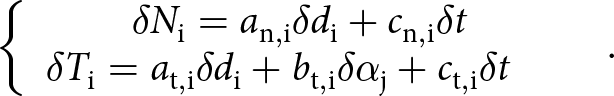 \begin{equation}\left\{ {\begin{array}{l}
\quad\,\,\,\,\,\,\,{\delta {N_{\text{i}}} = {a_{{\text{n}},{\text{i}}}}\delta {d_{\text{i}}} + {c_{{\text{n}},{\text{i}}}}\delta t\,\,\,\,\,\,\,\,\,\,\,\,\,\,\,\,} \\
{\delta {T_{\text{i}}} = {a_{{\text{t}},{\text{i}}}}\delta {d_{\text{i}}} + {b_{{\text{t}},{\text{i}}}}\delta {\alpha _{\text{j}}} + {c_{{\text{t}},{\text{i}}}}\delta t}
\end{array}} \right..\end{equation}
\begin{equation}\left\{ {\begin{array}{l}
\quad\,\,\,\,\,\,\,{\delta {N_{\text{i}}} = {a_{{\text{n}},{\text{i}}}}\delta {d_{\text{i}}} + {c_{{\text{n}},{\text{i}}}}\delta t\,\,\,\,\,\,\,\,\,\,\,\,\,\,\,\,} \\
{\delta {T_{\text{i}}} = {a_{{\text{t}},{\text{i}}}}\delta {d_{\text{i}}} + {b_{{\text{t}},{\text{i}}}}\delta {\alpha _{\text{j}}} + {c_{{\text{t}},{\text{i}}}}\delta t}
\end{array}} \right..\end{equation}Combining Eqns (5), (7) and (9) results in two sets of equations that provide the changes in the intergranular distances and in the opening angles as a function of the changes in the H-cell lengths:
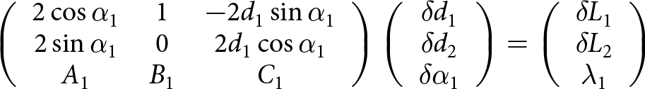 \begin{equation}\left( {\begin{array}{*{20}{c}}
{2\cos {\alpha _1}}&1&{ - 2{d_1}\sin {\alpha _1}} \\
{2\sin {\alpha _1}}&0&{2{d_1}\cos {\alpha _1}} \\
{{A_1}}&{{B_1}}&{{C_1}}
\end{array}} \right)\left( {\begin{array}{*{20}{c}}
{\delta {d_1}} \\
{\delta {d_2}} \\
{\delta {\alpha _1}}
\end{array}} \right) = \left( {\begin{array}{*{20}{c}}
{\delta {L_1}} \\
{\delta {L_2}} \\
{{\lambda _1}}
\end{array}} \right)\end{equation}
\begin{equation}\left( {\begin{array}{*{20}{c}}
{2\cos {\alpha _1}}&1&{ - 2{d_1}\sin {\alpha _1}} \\
{2\sin {\alpha _1}}&0&{2{d_1}\cos {\alpha _1}} \\
{{A_1}}&{{B_1}}&{{C_1}}
\end{array}} \right)\left( {\begin{array}{*{20}{c}}
{\delta {d_1}} \\
{\delta {d_2}} \\
{\delta {\alpha _1}}
\end{array}} \right) = \left( {\begin{array}{*{20}{c}}
{\delta {L_1}} \\
{\delta {L_2}} \\
{{\lambda _1}}
\end{array}} \right)\end{equation}and
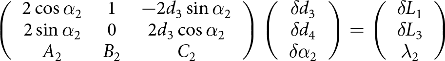 \begin{equation}\left( {\begin{array}{*{20}{c}}
{2\cos {\alpha _2}}&1&{ - 2{d_3}\sin {\alpha _2}} \\
{2\sin {\alpha _2}}&0&{2{d_3}\cos {\alpha _2}} \\
{{A_2}}&{{B_2}}&{{C_2}}
\end{array}} \right)\left( {\begin{array}{*{20}{c}}
{\delta {d_3}} \\
{\delta {d_4}} \\
{\delta {\alpha _2}}
\end{array}} \right) = \left( {\begin{array}{*{20}{c}}
{\delta {L_1}} \\
{\delta {L_3}} \\
{{\lambda _2}}
\end{array}} \right)\end{equation}
\begin{equation}\left( {\begin{array}{*{20}{c}}
{2\cos {\alpha _2}}&1&{ - 2{d_3}\sin {\alpha _2}} \\
{2\sin {\alpha _2}}&0&{2{d_3}\cos {\alpha _2}} \\
{{A_2}}&{{B_2}}&{{C_2}}
\end{array}} \right)\left( {\begin{array}{*{20}{c}}
{\delta {d_3}} \\
{\delta {d_4}} \\
{\delta {\alpha _2}}
\end{array}} \right) = \left( {\begin{array}{*{20}{c}}
{\delta {L_1}} \\
{\delta {L_3}} \\
{{\lambda _2}}
\end{array}} \right)\end{equation}with
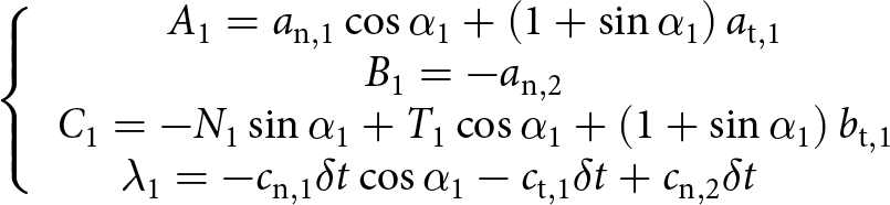 \begin{equation}\left\{ {\begin{array}{*{20}{c}}
{{A_1} = {a_{{\text{n}},1}}\cos {\alpha _1} + \left( {1 + \sin {\alpha _1}} \right){a_{{\text{t}},1}}} \\
\!\!\!{{B_1} = - {a_{{\text{n}},2}}} \\
{{C_1} = - {N_1}\sin {\alpha _1} + {T_1}\cos {\alpha _1} + \left( {1 + \sin {\alpha _1}} \right){b_{{\text{t}},1}}} \\
\!\!\!\!\!\!\!\!\!\!{{\lambda _1} = - {c_{{\text{n}},1}}\delta t\cos {\alpha _1} - {c_{{\text{t}},1}}\delta t + {c_{{\text{n}},2}}\delta t}
\end{array}} \right.\end{equation}
\begin{equation}\left\{ {\begin{array}{*{20}{c}}
{{A_1} = {a_{{\text{n}},1}}\cos {\alpha _1} + \left( {1 + \sin {\alpha _1}} \right){a_{{\text{t}},1}}} \\
\!\!\!{{B_1} = - {a_{{\text{n}},2}}} \\
{{C_1} = - {N_1}\sin {\alpha _1} + {T_1}\cos {\alpha _1} + \left( {1 + \sin {\alpha _1}} \right){b_{{\text{t}},1}}} \\
\!\!\!\!\!\!\!\!\!\!{{\lambda _1} = - {c_{{\text{n}},1}}\delta t\cos {\alpha _1} - {c_{{\text{t}},1}}\delta t + {c_{{\text{n}},2}}\delta t}
\end{array}} \right.\end{equation}and
 \begin{equation}\left\{ {\begin{array}{*{20}{c}}
{\,{A_2} = {a_{{\text{n}},3}}\cos {\alpha _2} + \left( {1 + \sin {\alpha _2}} \right){a_{{\text{t}},3}}} \\
\!\!{{B_2} = - {a_{{\text{n}},4}}} \\
{{C_2} = - {N_3}\sin {\alpha _2} + {T_3}\cos {\alpha _2} + \left( {1 + \sin {\alpha _2}} \right){b_{{\text{t}},2}}} \\
\!\!\!\!\!\!\!\!\!\!\!\!{{\lambda _2} = - {c_{{\text{n}},3}}\delta t\cos {\alpha _2} - {c_{{\text{t}},3}}\delta t + {c_{{\text{n}},4}}\delta t}
\end{array}} \right..\end{equation}
\begin{equation}\left\{ {\begin{array}{*{20}{c}}
{\,{A_2} = {a_{{\text{n}},3}}\cos {\alpha _2} + \left( {1 + \sin {\alpha _2}} \right){a_{{\text{t}},3}}} \\
\!\!{{B_2} = - {a_{{\text{n}},4}}} \\
{{C_2} = - {N_3}\sin {\alpha _2} + {T_3}\cos {\alpha _2} + \left( {1 + \sin {\alpha _2}} \right){b_{{\text{t}},2}}} \\
\!\!\!\!\!\!\!\!\!\!\!\!{{\lambda _2} = - {c_{{\text{n}},3}}\delta t\cos {\alpha _2} - {c_{{\text{t}},3}}\delta t + {c_{{\text{n}},4}}\delta t}
\end{array}} \right..\end{equation}The incremental contact forces can be obtained from the incremental intergranular distances and opening angles according to the incremental contact law (9).
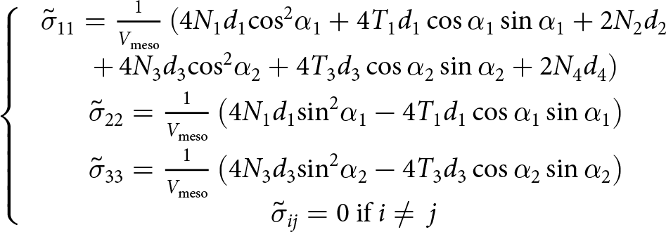
Continuing with the continuum formulation, the Love–Weber formula (Love, Reference Love1892) expresses the local stresses  $\underline {\underline {\widetilde {\boldsymbol{\sigma }}} } $ at the scale of the H-cell from the updated contact forces ${N_{\text{i}}}\left( t \right) = {N_{\text{i}}}\left( {t - {{\delta }}t} \right) + {{\delta }}{N_{\text{i}}}$ and ${T_{\text{i}}}\left( t \right) = {T_{\text{i}}}\left( {t - {{\delta }}t} \right) + {{\delta }}{T_{\text{i}}}$
 \begin{align}\left\{ {\begin{array}{*{20}{c}}
{\,{{\tilde \sigma }_{11}} = \frac{1}{{{V_{{\text{meso}}}}}}\left( {4{N_{\text{1}}}{d_1}{{\cos }^2}{\alpha _1} + 4{T_1}{d_1}\cos {\alpha _1}\sin {\alpha _1} + 2{N_2}{d_2}} \right.} \\[5pt]
{\left. {+\,4{N_{\text{3}}}{d_3}{{\cos }^2}{\alpha _2} + 4{T_3}{d_3}\cos {\alpha _2}\sin {\alpha _2} + 2{N_4}{d_4}} \right)} \\[3pt]
{\,{{\tilde \sigma }_{22}} = \frac{1}{{{V_{{\text{meso}}}}}}\left( {4{N_{\text{1}}}{d_1}{{\sin }^2}{\alpha _1} - 4{T_1}{d_1}\cos {\alpha _1}\sin \alpha_1} \right)} \\[7pt]
{\,{{\tilde \sigma }_{33}} = \frac{1}{{{V_{{\text{meso}}}}}}\left( {4{N_{\text{3}}}{d_3}{{\sin }^2}{\alpha _2} - 4{T_3}{d_3}\cos {\alpha _2}\sin \alpha_2} \right)}\\
{\tilde \sigma}_{ij}=0\ {\text{if}}\ i\neq\ j\\
\end{array}} \right.\nonumber\\ \end{align}
\begin{align}\left\{ {\begin{array}{*{20}{c}}
{\,{{\tilde \sigma }_{11}} = \frac{1}{{{V_{{\text{meso}}}}}}\left( {4{N_{\text{1}}}{d_1}{{\cos }^2}{\alpha _1} + 4{T_1}{d_1}\cos {\alpha _1}\sin {\alpha _1} + 2{N_2}{d_2}} \right.} \\[5pt]
{\left. {+\,4{N_{\text{3}}}{d_3}{{\cos }^2}{\alpha _2} + 4{T_3}{d_3}\cos {\alpha _2}\sin {\alpha _2} + 2{N_4}{d_4}} \right)} \\[3pt]
{\,{{\tilde \sigma }_{22}} = \frac{1}{{{V_{{\text{meso}}}}}}\left( {4{N_{\text{1}}}{d_1}{{\sin }^2}{\alpha _1} - 4{T_1}{d_1}\cos {\alpha _1}\sin \alpha_1} \right)} \\[7pt]
{\,{{\tilde \sigma }_{33}} = \frac{1}{{{V_{{\text{meso}}}}}}\left( {4{N_{\text{3}}}{d_3}{{\sin }^2}{\alpha _2} - 4{T_3}{d_3}\cos {\alpha _2}\sin \alpha_2} \right)}\\
{\tilde \sigma}_{ij}=0\ {\text{if}}\ i\neq\ j\\
\end{array}} \right.\nonumber\\ \end{align} where  ${V_{{\text{meso}}}}$ is the external volume of the mesostructure (Wautier, Reference Wautier2021). Finally, a statistical homogenization of the stresses over the complete H-cell collection provides the stress tensor $\underline {\underline {\boldsymbol{\sigma }} } $ in the global frame:
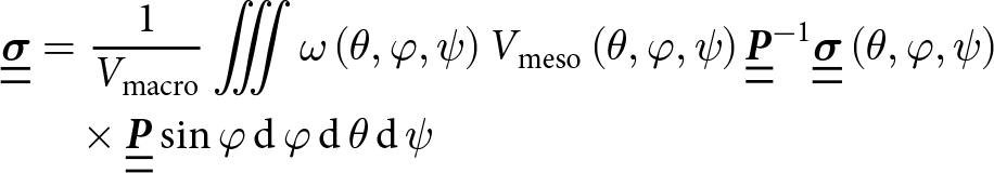 \begin{align}\underline {\underline {\boldsymbol{\sigma }} } &= \frac{1}{{{V_{{\text{macro}}}}}}\iiint \omega \left( {\theta ,\varphi ,\psi } \right){V_{{\text{meso}}}}\left( {\theta ,\varphi ,\psi } \right){{\underline {\underline {\boldsymbol{P}} } }^{ - 1}}{ }\underline {\underline {\boldsymbol{\sigma }} } \left( {\theta ,\varphi ,\psi } \right){ } \nonumber\\ &\quad\times\underline {\underline {\boldsymbol{P}} } \sin \varphi\,{\text{d}}\,\varphi\,{\text{d}}\,\theta\,{\text{d}}\,\psi \end{align}
 where  $\omega \left( {\theta ,\varphi ,\psi } \right)$ is the probability density function of the H-cell distribution, which satisfies:
 \begin{equation}\iiint {\omega \left( {\theta ,\varphi ,\psi } \right)\sin \varphi\,{\text{d}}\,\varphi\,{\text{d}}\,\theta\,{\text{d}}\,\psi } = 1\end{equation}
 and  ${V_{{\text{macro}}}}$ is the total volume of the distribution of H-cells given by:
 \begin{equation}{V_{{\text{macro}}}} = \iiint {\omega \left( {\theta ,\varphi ,\psi } \right){V_{{\text{meso}}}}\left( {\theta ,\varphi ,\psi } \right)\sin \varphi\,{\text{d}}\,\varphi\,{\text{d}}\,\theta\,{\text{d}}\,\psi}.\end{equation}
Eventually, we obtain a multi-scale constitutive model that relates the total stress to the global strain under an incremental formalism (Fig. 3). The hypothesis of non-correlated mesostructures inferred by the statistical homogenization, and the hypothesis on the geometry of the mesostructure could lead to an error, but previous works on the H-model (Nicot and Darve, Reference Nicot and Darve2011; Xiong and others, Reference Xiong, Nicot and Yin2017; Veylon and others, Reference Veylon, Nicot, Zhu and Darve2018; Wautier, Reference Wautier2021; Xiong, Reference Xiong2021; Deng, Reference Deng2022; Liu and others, Reference Liu, Nicot, Wautier and Darve2024) have proven that this error is not significant.
2.2. Contact law between ice grains
In the extended version of the 3-D H-model proposed hereafter, the snow constitutive features are accounted for by introducing a specific contact law between the ice grains of each hexagon of a H-cell. In the context of the snow-H-model, the history of a contact is supposed to be the following:
(i) The ice grains have undergone metamorphism processes which progressively round their shape (Fierz, Reference Fierz2009). Ice grains are thus assumed to be spherical.
(ii) Thermodynamic sintering has created viscous ice bonds at all contacts between ice grains (Kabore and others, Reference Kabore, Peters, Michael and Nicot2021) (Peters and others, Reference Peters, Kabore, Michael and Nicot2021). Each ice bond is assumed to be incompressible (Lipovsky, Reference Lipovsky2022), meaning that its volume originates only from the prior sintering conditions, such as temperature and sintering time (Szabo and Schneebeli, Reference Szabo and Schneebeli2007).
(iii) Bond creation processes are supposed to be slow compared to the loading rates considered in the targeted applications ( $\dot \varepsilon { } \geqslant {10^{ - 4}}{ }{{\text{s}}^{ - 1}}$). Consequently, if an ice bond fails during the stress loading, it has no time to reform, and the contact becomes cohesionless until the end of the loading.

Based on these assumptions, the contact law to be developed in the snow-H-model must account for both bonded and unbonded contacts between spherical ice grains.
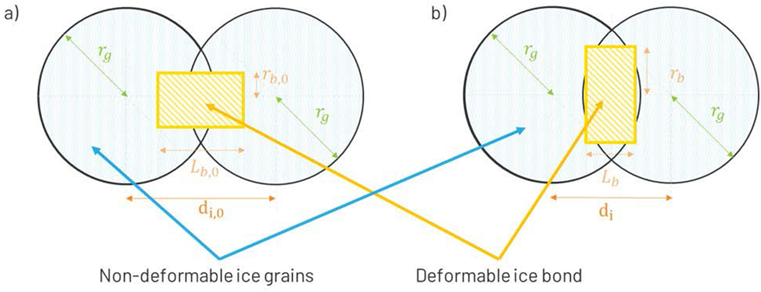
Grains in contact are assumed to be initially bonded by a cylindrical ice bridge resulting from prior snow metamorphism (Fig. 4). The bridge is characterized by its radius  ${r_{\text{b}}}$ and its length ${L_{\text{b}}}$, with ${r_{{\text{b}},0}}$ and ${L_{{\text{b}},0}}$ their respective values at the initial time step. Note that the initial bond geometry before loading created by prior thermodynamic sintering can be changed through its initial radius, enabling the modelling of different snow types (Szabo and Schneebeli, Reference Szabo and Schneebeli2007). During mechanical loading, the strain is assumed to be localized into the cylindrical ice bonds while the spherical ice grains are assumed perfectly rigid so that the strain is fully concentrated within the bond.
Schematic representation of a bonded contact: (a) initially after snow metamorphism and before loading; (b) during the loading. The yellow hatched zones represent the deformable ice bond, and the blue dotted zones represent the non-deformable parts of the ice grains.
The deformable bond between two ice grains is modelled by a Maxwell elasto-viscoplastic beam on the basis of the work of Kabore and others (Reference Kabore, Peters, Michael and Nicot2021) and Peters and others (Reference Peters, Kabore, Michael and Nicot2021). The main discrepancy with this model lies in the absence of grain rotation in the H-model which leads to the lack of torsion and bending in the ice beam. The creep behaviour of ice, which can be dominant during loading, is accounted for by introducing viscoplasticity in the bond.
The total normal bond strain  $\varepsilon_{{\text{b}},{\text{n}}}^{{\text{tot}}}$ can be split into an elastic part $\varepsilon_{{\text{b}},{\text{n}}}^{\text{e}}$ and a viscoplastic part $\varepsilon _{{\text{b}},{\text{n}}}^{{\text{vp}}}$:
 \begin{equation}\varepsilon _{{\text{b}},{\text{n}}}^{{\text{tot}}} = \varepsilon _{{\text{b}},{\text{n}}}^{{\text{vp}}} + \varepsilon _{{\text{b}},{\text{n}}}^{\text{e}}\end{equation}
 The viscoplastic deformation accounts for the well-known creep behaviour of ice since the creep rate  $\dot \varepsilon _{{\text{b}},{\text{n}}}^{{\text{vp}}}$ in the bond direction is related to the normal stress ${\sigma _{{\text{b}},{\text{n}}}}$ by Glen’s law (Barnes and others, Reference Barnes, Tabor and Walker1971):
 \begin{equation}\dot \varepsilon _{{\text{b}},{\text{n}}}^{{\text{vp}}} = \frac{{{{\delta }}\varepsilon _{{\text{b}},{\text{n}}}^{{\text{vp}}}}}{{{{\delta }}t}} = A\left( {{T_{{\text{emp}}}}} \right)\sigma _{{\text{b}},{\text{n}}}^m\end{equation}
 where  $A\left( {{T_{{\text{emp}}}}} \right)$ is a temperature dependent coefficient, and $m$ is an exponent generally close to 3 (Barnes and others, Reference Barnes, Tabor and Walker1971).
Finally, the elastic normal deformation is simply proportional to the normal stress. Due to the adhesion of the bond on the ice grains (which prevents the bond from expanding laterally around the contact points), using Young’s modulus  $E\,$ would underestimate the stiffness of the bond/grains assembly. Thus, the oedometer coefficient of ice ${E_{{\text{oedo}}}}$ is used instead to better reflect the lateral geometrical constraints:
 \begin{equation}{\sigma _{{\text{b}},{\text{n}}}} = \frac{{E\left( {1 - \nu } \right)}}{{\left( {1 + \nu } \right)\left( {1 - 2\nu } \right)}}\varepsilon _{{\text{b}},{\text{n}}}^{\text{e}} = {E_{{\text{oedo}}}}\varepsilon _{{\text{b}},{\text{n}}}^{\text{e}}\end{equation}
 with  $\nu $ the Poisson’s ratio of ice.
The normal strain in the bond can be expressed as a function of the bond length, thanks to the strain localization assumption:
 \begin{equation}\varepsilon _{{\text{b}},{\text{n}}}^{{\text{tot}}} = - \frac{{{L_{\text{b}}} - {L_{{\text{b}},0}}}}{{{L_{{\text{b}},0}}}}\end{equation}
 with  ${L_{\text{b}}}$ and ${L_{{\text{b}},0}}$ being the bond length, respectively, at the current time and at the beginning of the loading. It should be noted that compression and contraction are counted positive.
The normal stress can be related to the normal contact force  ${N^{\text{b}}}$ as follows:
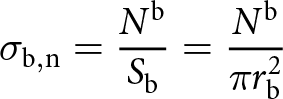 \begin{equation}{\sigma _{{\text{b}},{\text{n}}}} = \frac{{{N^{\text{b}}}}}{{{S_{\text{b}}}}} = \frac{{{N^{\text{b}}}}}{{{{\pi }}r_{\text{b}}^2}}\end{equation}
 where  ${r_{\text{b}}}$ is the radius of the cylindrical bond and ${S_{\text{b}}}$ its section.
As the bond is the only deformable element in the bonded ice grain model, the incremental bond length  ${{\delta }}{L_{\text{b}}}$ is directly equal to the incremental intergranular distance ${{\delta }}d$:
 \begin{equation}{{\delta }}{L_{\text{b}}} = {{\delta }}d\end{equation}
Eventually, the incompressibility condition, together with the volume conservation of the ice bond, read:
 \begin{equation}{{\pi }}{r_{\text{b}}}^2{L_{\text{b}}} = {{\pi }}{r_{{\text{b}},0}}^2{L_{{\text{b}},0}}\end{equation}
 By combining Eqns (18)–(24), the contact law relating the incremental normal contact force  ${{\delta }}{N^{\text{b}}}$ to the incremental intergranular distance ${{\delta }}d$ can be obtained:
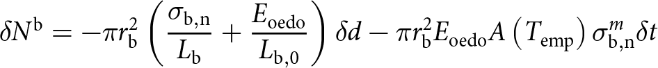 \begin{align}{{\delta }}{N^{\text{b}}} = - {{\pi }}r_{\text{b}}^2\left( {\frac{{{\sigma _{{\text{b}},{\text{n}}}}}}{{{L_{\text{b}}}}} + \frac{{{E_{{\text{oedo}}}}}}{{{L_{{\text{b}},0}}}}} \right){{\delta }}d - {{\pi }}r_{\text{b}}^2{E_{{\text{oedo}}}}A\left( {{T_{{\text{emp}}}}} \right)\sigma _{{\text{b}},{\text{n}}}^m{{\delta }}t\nonumber\\ \end{align}
 Likewise, the incremental tangential contact force can be expressed as a function of the incremental intergranular distance and of the variation of the bond direction, characterized by  ${{\delta }}\alpha $:
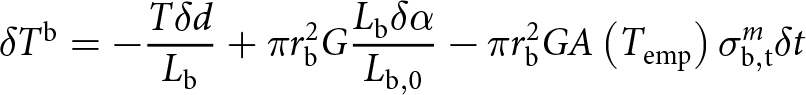 \begin{equation}{{\delta }}{T^{\text{b}}} = - \frac{{T{{\delta }}d}}{{{L_{\text{b}}}}} + {{\pi }}r_{\text{b}}^2G\frac{{{L_{\text{b}}}{{\delta }}\alpha }}{{{L_{{\text{b}},0}}}} - {{\pi }}r_{\text{b}}^2GA\left( {{T_{{\text{emp}}}}} \right)\sigma _{{\text{b}},{\text{t}}}^m{{\delta }}t\end{equation}
 with  $G = \frac{E}{{2\left( {1 + \nu } \right)}}$ the shear modulus of ice. The way to obtain this expression using Glen’s law is detailed in Appendix A.
During the loading, stresses increase in the bond, which can lead to its failure. In our approach, only brittle failure is accounted for as the strain rate in the targeted engineering applications is supposed to be high enough ( $\dot \varepsilon \geqslant {10^{ - 4}}{{\text{s}}^{ - 1}}$). Brittle bond failure occurs as soon as one of the following conditions is met:
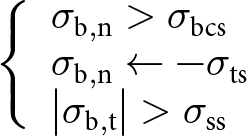 \begin{equation}\left\{ {\begin{array}{l}
{{\sigma _{{\text{b}},{\text{n}}}} \gt {\sigma _{{\text{bcs}}}}} \\
{{\sigma _{{\text{b}},{\text{n}}}} \leftarrow - {\sigma _{{\text{ts}}}}} \\
{\left| {{\sigma _{{\text{b}},{\text{t}}}}} \right| \gt {\sigma _{{\text{ss}}}}}
\end{array}} \right.\end{equation}
\begin{equation}\left\{ {\begin{array}{l}
{{\sigma _{{\text{b}},{\text{n}}}} \gt {\sigma _{{\text{bcs}}}}} \\
{{\sigma _{{\text{b}},{\text{n}}}} \leftarrow - {\sigma _{{\text{ts}}}}} \\
{\left| {{\sigma _{{\text{b}},{\text{t}}}}} \right| \gt {\sigma _{{\text{ss}}}}}
\end{array}} \right.\end{equation} where  ${\sigma _{{\text{b}},{\text{n}}}}$ is the normal stress in the bond, which is positive in compression, ${\sigma _{{\text{b}},{\text{t}}}}$ is the shear stress in the bond. ${\sigma _{{\text{bcs}}}}$, ${\sigma _{{\text{ts}}}}$ and ${\sigma _{{\text{ss}}}}$ are respectively the compression, tensile and shear strength of ice (see Figure 5). The expression of the brittle strengths of the ice bonds is given by Michael (Reference Michael2014) and Kabore and others (Reference Kabore, Peters, Michael and Nicot2021):
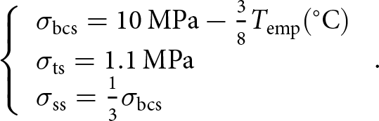 \begin{equation}\left\{ {\begin{array}{l}
{{\sigma _{{\text{bcs}}}} = 10\,\text{MPa} - \frac{3}{8}{T_{{\text{emp}}}}{(^ \circ }\text{C})} \\
{{\sigma _{{\text{ts}}}} = 1.1\,\text{MPa}\,\,\,\,\,\,\,\,\,\,\,\,\,\,\,\,\,\,\,\,\,\,\,\,\,\,} \\
{{\sigma _{{\text{ss}}}} = \frac{1}{3}{\sigma _{{\text{bcs}}}}\,\,\,\,\,\,\,\,\,\,\,\,\,\,\,\,\,\,\,\,\,\,\,\,\,\,\,\,\,\,\,}
\end{array}} \right..\end{equation}
\begin{equation}\left\{ {\begin{array}{l}
{{\sigma _{{\text{bcs}}}} = 10\,\text{MPa} - \frac{3}{8}{T_{{\text{emp}}}}{(^ \circ }\text{C})} \\
{{\sigma _{{\text{ts}}}} = 1.1\,\text{MPa}\,\,\,\,\,\,\,\,\,\,\,\,\,\,\,\,\,\,\,\,\,\,\,\,\,\,} \\
{{\sigma _{{\text{ss}}}} = \frac{1}{3}{\sigma _{{\text{bcs}}}}\,\,\,\,\,\,\,\,\,\,\,\,\,\,\,\,\,\,\,\,\,\,\,\,\,\,\,\,\,\,\,}
\end{array}} \right..\end{equation}Different modes of bond failure (tensile, compression and shear). Note that potential additional failure modes by bending and torsion are not accounted for as rotation of the grains is not possible in the H-model.

When bond failure occurs, the contact law between the ice grains is reduced to a simple elasto-plastic law:
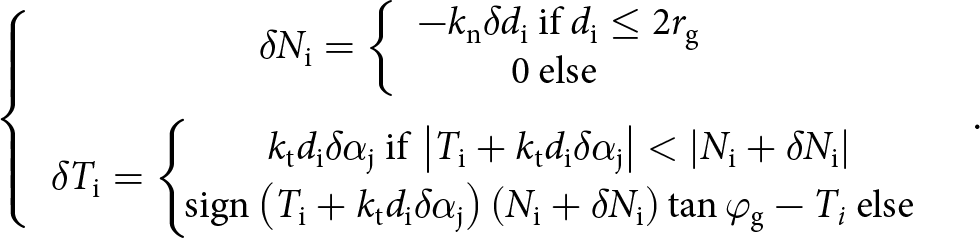 \begin{align}\left\{ {\begin{array}{c}
{\delta {N_{\text{i}}} = \left\{ {\begin{array}{*{20}{c}}
{- {k_{\text{n}}}{{\delta }}{d_{\text{i}}}{\text{ if }}{d_{\text{i}}} \leq 2{r_{\text{g}}}} \\
{0{\text{ else }}}
\end{array}} \right.\,} \\[12pt]
{\delta {T_{\text{i}}} = \left\{ {\begin{array}{*{20}{c}}
{{k_{\text{t}}}{d_{\text{i}}}{{\delta }}{\alpha _{\text{j}}}{\text{ if }}\left| {{T_{\text{i}}} + {k_{\text{t}}}{d_{\text{i}}}{{\delta }}{\alpha _{\text{j}}}} \right| \lt \left| {{N_{\text{i}}} + {{\delta }}{N_{\text{i}}}} \right|{ }} \\[3pt]
{\!\!\!\!{\text{sign}}\left( {{T_{\text{i}}} + {k_{\text{t}}}{d_{\text{i}}}{{\delta }}{\alpha _{\text{j}}}} \right)\left( {{N_{\text{i}}} + {{\delta }}{N_{\text{i}}}} \right)\tan {\varphi _{\text{g}}} - {T_i}{\text{ else}}}
\end{array}} \right.}
\end{array}} \right..\nonumber\\ \end{align}
\begin{align}\left\{ {\begin{array}{c}
{\delta {N_{\text{i}}} = \left\{ {\begin{array}{*{20}{c}}
{- {k_{\text{n}}}{{\delta }}{d_{\text{i}}}{\text{ if }}{d_{\text{i}}} \leq 2{r_{\text{g}}}} \\
{0{\text{ else }}}
\end{array}} \right.\,} \\[12pt]
{\delta {T_{\text{i}}} = \left\{ {\begin{array}{*{20}{c}}
{{k_{\text{t}}}{d_{\text{i}}}{{\delta }}{\alpha _{\text{j}}}{\text{ if }}\left| {{T_{\text{i}}} + {k_{\text{t}}}{d_{\text{i}}}{{\delta }}{\alpha _{\text{j}}}} \right| \lt \left| {{N_{\text{i}}} + {{\delta }}{N_{\text{i}}}} \right|{ }} \\[3pt]
{\!\!\!\!{\text{sign}}\left( {{T_{\text{i}}} + {k_{\text{t}}}{d_{\text{i}}}{{\delta }}{\alpha _{\text{j}}}} \right)\left( {{N_{\text{i}}} + {{\delta }}{N_{\text{i}}}} \right)\tan {\varphi _{\text{g}}} - {T_i}{\text{ else}}}
\end{array}} \right.}
\end{array}} \right..\nonumber\\ \end{align} In the absence of ice bond, the normal stiffness  ${k_{{\text{n}},{\text{i}}}}$ between ice grains at contact $i\,$ evolves with grain interpenetration (see justification in Appendix B):
 \begin{equation}{k_{{\text{n}},{\text{i}}}} = {E_{{\text{ice}}}}\frac{{{\pi }}}{2}\left( {{r_{\text{g}}} - \frac{{d_{\text{i}}^2}}{{4{r_{\text{g}}}}}} \right).\end{equation}
2.3. Extension of the 3-D H-model to snow
The relationship between the incremental contact forces and the changes in the local kinematics (including the intergranular distances between two ice grains and the contact direction) has been previously established in Section 2.2, both for a bonded contact (Eqns (25) and (26)) and after failure of the ice bond (Eqn (29)). The incremental normal contact force in Eqns (25) and (29) and the incremental tangential force in Eqns (26) and (29) can be written generically as in Eqn (9), with the corresponding coefficients:
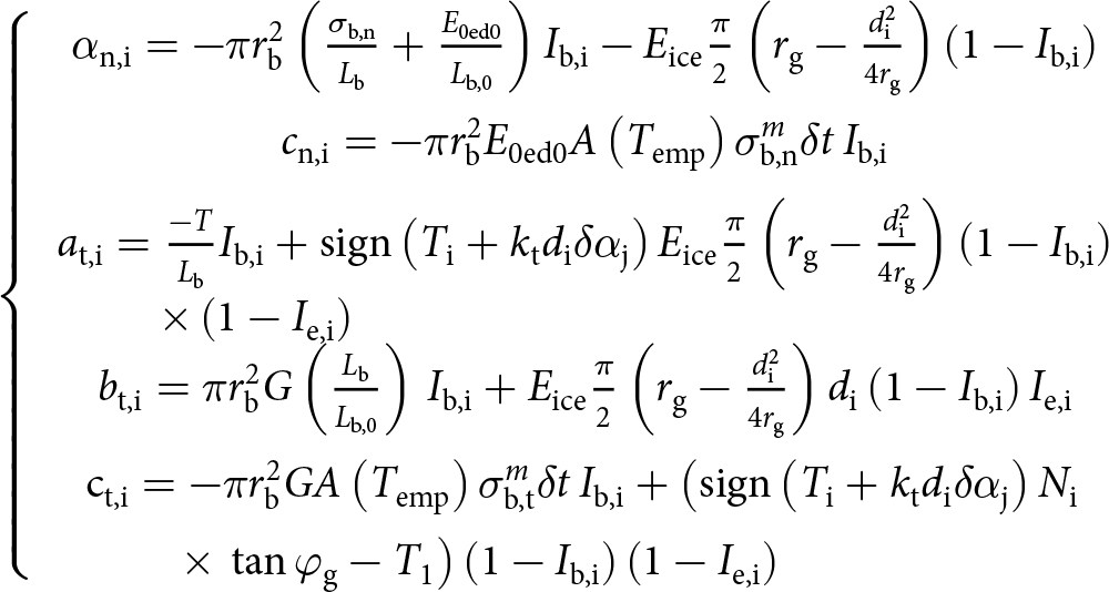 \begin{align}\left\{ {\begin{array}{*{20}{c}}
{\alpha _{{\text{n,i}}}} = - {{\pi }}r_{\text{b}}^2\left( {\frac{{{\sigma _{{\text{b,n}}}}}}{{{L_{\text{b}}}}} + \frac{{{E_{{\text{0ed0}}}}}}{{{L_{{\text{b,0}}}}}}} \right){I_{{\text{b,i}}}} - {E_{{\text{ice}}}}\frac{{{\pi }}}{2}\left( {{r_{\text{g}}} - \frac{{d_{\text{i}}^2}}{{4{r_{\text{g}}}}}} \right) \left( {1 - {I_{{\text{b,i}}}}} \right) \\[10pt]
{{c_{{\text{n,i}}}} = - {{\pi }}r_{\text{b}}^2{E_{{\text{0ed0}}}}A\left( {{T_{{\text{emp}}}}} \right)\sigma _{{\text{b,n}}}^m\delta t\,{I_{{\text{b,i}}}}} \\[7pt]
{a_{{\text{t,i}}}} = \frac{-T}{{{L_{\text{b}}}}}{I_{{\text{b,i}}}} + {\text{sign}}\left( {{T_{\text{i}}} + {k_{\text{t}}}{d_{\text{i}}}\delta {\alpha _{\text{j}}}} \right){E_{{\text{ice}}}}\frac{{{\pi }}}{2}\left( {{r_{\text{g}}} - \frac{{d_{\text{i}}^2}}{{4{r_{\text{g}}}}}} \right)\left( {1 - {I_{{\text{b,i}}}}} \right)\\ \times\left( {1 - {I_{{\text{e,i}}}}} \right)\quad\qquad\qquad\qquad\qquad\qquad\qquad\qquad\quad \\
{b_{{\text{t,i}}}} = {{\pi }}r_{\text{b}}^2G\left( {\frac{{{L_{\text{b}}}}}{{{L_{{\text{b,0}}}}}}} \right)\,{I_{{\text{b,i}}}} + {E_{{\text{ice}}}}\frac{{{\pi }}}{2}\left( {{r_{\text{g}}} - \frac{{d_{\text{i}}^2}}{{4{r_{\text{g}}}}}} \right){d_{\text{i}}}\left( {1 - {I_{{\text{b,i}}}}} \right){I_{{\text{e,i}}}} \\[10pt]
{{\text{c}}_{{\text{t,i}}}} = - {{\pi }}r_{\text{b}}^2GA\left( {{T_{{\text{emp}}}}} \right)\sigma _{{\text{b,t}}}^m\delta t\,{I_{{\text{b,i}}}} + \left( {\text{sign}}\left( {{T_{\text{i}}} + {k_{\text{t}}}{d_{\text{i}}}\delta {\alpha _{\text{j}}}} \right){N_{\text{i}}} \right.\\[6pt] \quad{} \times\left.{\text{tan}}\,{\varphi _{\text{g}}} - {T_{\text{1}}} \right)\left( {1 - {I_{{\text{b,i}}}}} \right)\left( {1 - {I_{{\text{e,i}}}}} \right)\qquad\qquad\quad\quad\quad
\end{array}} \right.\nonumber\\ \end{align}
\begin{align}\left\{ {\begin{array}{*{20}{c}}
{\alpha _{{\text{n,i}}}} = - {{\pi }}r_{\text{b}}^2\left( {\frac{{{\sigma _{{\text{b,n}}}}}}{{{L_{\text{b}}}}} + \frac{{{E_{{\text{0ed0}}}}}}{{{L_{{\text{b,0}}}}}}} \right){I_{{\text{b,i}}}} - {E_{{\text{ice}}}}\frac{{{\pi }}}{2}\left( {{r_{\text{g}}} - \frac{{d_{\text{i}}^2}}{{4{r_{\text{g}}}}}} \right) \left( {1 - {I_{{\text{b,i}}}}} \right) \\[10pt]
{{c_{{\text{n,i}}}} = - {{\pi }}r_{\text{b}}^2{E_{{\text{0ed0}}}}A\left( {{T_{{\text{emp}}}}} \right)\sigma _{{\text{b,n}}}^m\delta t\,{I_{{\text{b,i}}}}} \\[7pt]
{a_{{\text{t,i}}}} = \frac{-T}{{{L_{\text{b}}}}}{I_{{\text{b,i}}}} + {\text{sign}}\left( {{T_{\text{i}}} + {k_{\text{t}}}{d_{\text{i}}}\delta {\alpha _{\text{j}}}} \right){E_{{\text{ice}}}}\frac{{{\pi }}}{2}\left( {{r_{\text{g}}} - \frac{{d_{\text{i}}^2}}{{4{r_{\text{g}}}}}} \right)\left( {1 - {I_{{\text{b,i}}}}} \right)\\ \times\left( {1 - {I_{{\text{e,i}}}}} \right)\quad\qquad\qquad\qquad\qquad\qquad\qquad\qquad\quad \\
{b_{{\text{t,i}}}} = {{\pi }}r_{\text{b}}^2G\left( {\frac{{{L_{\text{b}}}}}{{{L_{{\text{b,0}}}}}}} \right)\,{I_{{\text{b,i}}}} + {E_{{\text{ice}}}}\frac{{{\pi }}}{2}\left( {{r_{\text{g}}} - \frac{{d_{\text{i}}^2}}{{4{r_{\text{g}}}}}} \right){d_{\text{i}}}\left( {1 - {I_{{\text{b,i}}}}} \right){I_{{\text{e,i}}}} \\[10pt]
{{\text{c}}_{{\text{t,i}}}} = - {{\pi }}r_{\text{b}}^2GA\left( {{T_{{\text{emp}}}}} \right)\sigma _{{\text{b,t}}}^m\delta t\,{I_{{\text{b,i}}}} + \left( {\text{sign}}\left( {{T_{\text{i}}} + {k_{\text{t}}}{d_{\text{i}}}\delta {\alpha _{\text{j}}}} \right){N_{\text{i}}} \right.\\[6pt] \quad{} \times\left.{\text{tan}}\,{\varphi _{\text{g}}} - {T_{\text{1}}} \right)\left( {1 - {I_{{\text{b,i}}}}} \right)\left( {1 - {I_{{\text{e,i}}}}} \right)\qquad\qquad\quad\quad\quad
\end{array}} \right.\nonumber\\ \end{align} where  ${\text{i}}$ stands for the number of the considered contact, as defined in Fig. 2. ${I_{{\text{b}},{\text{i}}}}$ is a bond indicator equal to one when the ice bond at contact ${\text{i}}$ exists, and zero otherwise. ${I_{{\text{e}},{\text{i}}}}$ is a similar indicator which is equal to one in a nonbonded elastic contact, and zero otherwise. The ice contact law defined by these coefficients can be implemented readily within the standard computation scheme of the H-model. Some additional improvements of the model in relation with the creation and the loss of contacts in the H-cell are described in Appendix C and D.
3. Homogeneous compression test simulations
In this section, the snow-H-model is validated at the representative elementary volume (REV) scale against experimental tests by (Abele and Gow, Reference Abele and Gow1976) conducted for different snow types. The numerical parameters are tuned to match the experimental stress/strain curves as closely as possible. This calibration procedure enables to identify the snow density range over which the model can capture the mechanical response of snow.
3.1. Confined compression test
In Abele and Gow (Reference Abele and Gow1976), several confined compression tests were performed on different snow samples. In practice, natural snow was collected in cylindrical containers and compacted at temperatures ranging between  $ - 7^\circ {\text{C}}$ and $ - 1^\circ {\text{C}}$. The snow samples were then stored for 0.1–7 days before being tested under oedometer conditions at a constant temperature between $ - 34^\circ {\text{C}}$ and $ - 1^\circ {\text{C}}$. The storage duration prior to testing is referred to as the snow age in the following. During the compression test, a vertical velocity of
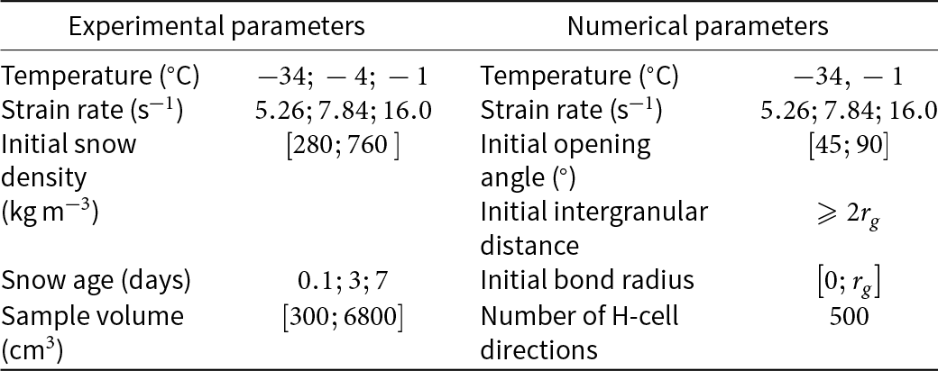
  $40{\text{ cm}}/{\text{s}}$ was applied to the top of the sample, while lateral deformations were kept constant. The experimental parameters are summarized in the first two columns of Table 1. The initial snow density of each sample was determined from the original volume and after measurement of the final sample weight.
Experimental (left) and numerical parameters (right) for confined compression tests on snow (Abele and Gow, Reference Abele and Gow1976)
3.2. Calibration against experimental results
The extension of the 3-D H-model to snow is implemented in a stand-alone Python code which is used to run REV scale tests under strain-controlled conditions. The compression tests under lateral confining from Abele and Gow (Reference Abele and Gow1976) are reproduced with this code.
Some of the experimental parameters of the experiments such as the snow temperature and the strain rate can be directly used in the simulations. However, the initial snow density and the snow age are not explicit input parameters for the 3-D H-model. The experimental snow age is only indirectly related to the initial bond radius  ${{\text{r}}_{{\text{b}},0}}$ (Szabo and Schneebeli, Reference Szabo and Schneebeli2007) and the initial density derives from the initial geometry of the H-cells. The latter is determined by the initial opening angle
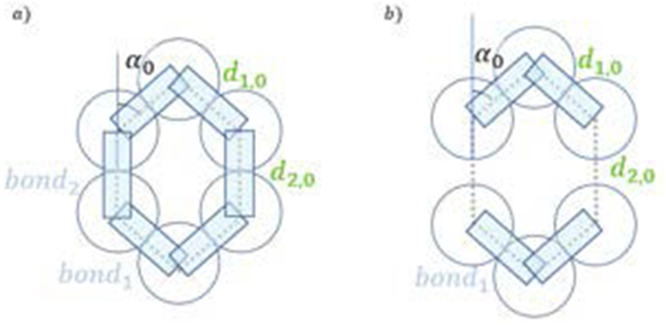
  ${\alpha _{1,0}} = {\alpha _{2,0}} = {\alpha _0}$ which can be varied to modify the initial density. Unlike the original H-model for sand, some grains may not necessarily be in contact in the snow-H-model (see Fig. 6), to account for large porosity values in snow. A new parameter is then introduced: the initial inter-granular distance ${d_{2,0}}$ (see Fig. 6 where ${d_{2,0}} = {d_{4,0}} \geq 2{r_{\text{g}}}$ and Appendix D). In the case where ${d_{2,0}} = {d_{4,0}} \geq 2{r_{\text{g}}}$, the connectivity of forces within the cell is maintained through contact with neighbouring cells. This is reflected by the external force $F_1^a$ being balanced by the tangential external force ${G_2}$ (see Fig. 2), resulting in the equilibrium of the two half cells (see Appendix D). As a result, the initial density in the experiments can be accounted for by calibrating the two numerical parameters ${d_{2,0}}$ and ${\alpha _0}$. The sintering time before loading is included in the snow-H-model from the initial bond radius ${r_{{\text{b}},0}}$, which is capped by the grain radius. The numerical parameters and their range of variation are summarized in the last two columns of Table 1.
Initial configurations of a hexagonal mesostructure: (a) 2-D representation of a ten-grain H-cell with  ${d_{2,0}} = {d_{1,0}} = 2{r_{\text{g}}}$ and initial ice bonds ${\text{bon}}{{\text{d}}_1}$ and ${\text{bon}}{{\text{d}}_2}$; (b) 2-D representation of two separated five-grain mesostructure with ${d_{1,0}} = 2{r_{\text{g}}}$, ${d_{2,0}} \gt 2{r_{\text{g}}}$ and initial bonds ${\text{bon}}{{\text{d}}_1}$.
The first objective of the calibration step is to determine the initial value of the three numerical parameters describing both the geometry and the sintering state of the H-cell, namely the opening angle  ${\alpha _0}$, the intergranular distance ${d_{2,0}}$ and the bond radius ${r_{{\text{b}},0}}$. To this end, stress–strain curves for different initial parameters are systematically compared to the experimental curves by Abele and Gow (Reference Abele and Gow1976). The best fitting triplet $\left( {{\text{denoted by the index bf}}} \right)$ in the parameter set ${{\Omega }}$ given in Table 1 corresponds to the triplet ${\left( {{\alpha _0},{d_{2,0}},{r_{{\text{b}},0}}} \right)_{{\text{bf}}}}$ which verifies:
 \begin{equation}{\text{err}}{\left( {{\alpha _0},{d_{2,0}},{r_{{\text{b}},0}}} \right)_{{\text{bf}}}} = \mathop {\min }\limits_{{\Omega }} \left( {{\text{err}}\left( {{\alpha _0},{d_{2,0}},{r_{{\text{b}},0}}} \right)} \right)\end{equation}
 with  ${\text{err}}$ being a relative error gap function defined by:
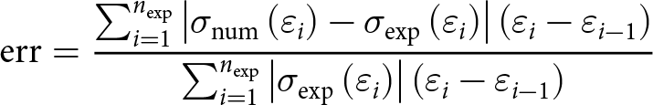 \begin{equation}{\text{err}} = \frac{{{{\mathop \sum}}_{i = 1}^{{n_{{\text{exp}}}}}\left| {{\sigma _{{\text{num}}}}\left( {{\varepsilon _i}} \right) - {\sigma _{{\text{exp}}}}\left( {{\varepsilon _i}} \right)} \right|\left( {{\varepsilon _i} - {\varepsilon _{i - 1}}} \right)}}{{{{\mathop \sum }}_{i = 1}^{{n_{{\text{exp}}}}}\left| {{\sigma _{{\text{exp}}}}\left( {{\varepsilon _i}} \right)} \right|\left( {{\varepsilon _i} - {\varepsilon _{i - 1}}} \right)}}\end{equation}
 In Eqn (33), the numerator corresponds to the cumulated area between the numerical and experimental curves in the axial stress–strain space  $\left( {\sigma ,\varepsilon } \right)$, whereas the denominator corresponds to the area below the experimental curve. ${n_{{\text{exp}}}}$ is the number of points taken from the experimental stress–strain curve, ${\varepsilon _i}$ is the strain at the ith point of the experimental curve, ${\sigma _{{\text{num}}}}$ is the stress obtained with the 3-D H-model and ${\sigma _{{\text{exp}}}}$ is the experimental one.
The parameter set in  ${{\Omega }} = \{ {( {{\alpha _0},{d_{2,0}},{r_{{\text{b}}0}}} ) \in [ {{{45}^ \circ };{{90}^ \circ }} ] \times }$ ${[ {2{ }{r_{\text{g}}};{ }3.6{ }{r_{\text{g}}}} ] \times [ {0.05{ }{r_{\text{g}}};0.9{ }{r_{\text{g}}}} ]} \}$ has been explored for experimental curves corresponding to a density between $470{\text{ kg}}/{{\text{m}}^3}$ and $640{\text{ kg}}/{{\text{m}}^3}$. The stress–strain curves of the experimental data and the corresponding best fitting numerical curves in ${{\Omega }}$ are reported in Fig. 7.
Stress–strain curves for confined compression test: experimental results from Abele and Gow (Reference Abele and Gow1976) and best fitting numerical curves obtained with the 3-D H-model.

Table 2 reports the best fit parameters with the initial density of the experimental specimens increasing from  $470{\text{ kg}}/{{\text{m}}^3}$ to $640{\text{ kg}}/{{\text{m}}^3}$. The relative error gap, as defined in Eqn (33), ranges between $1.4{ }$% and $12.3{\text{\% }}$.
Parameters giving the best fit for each experimental curve in  $\boldsymbol{\Omega} = \left[ {{{45}^ \circ };{{90}^ \circ }} \right] \times \left[ {2\,{r_g};\,3.6\,{r_g}} \right] \times \left[ {0.05\,{r_g};0.9\,{r_g}} \right].$
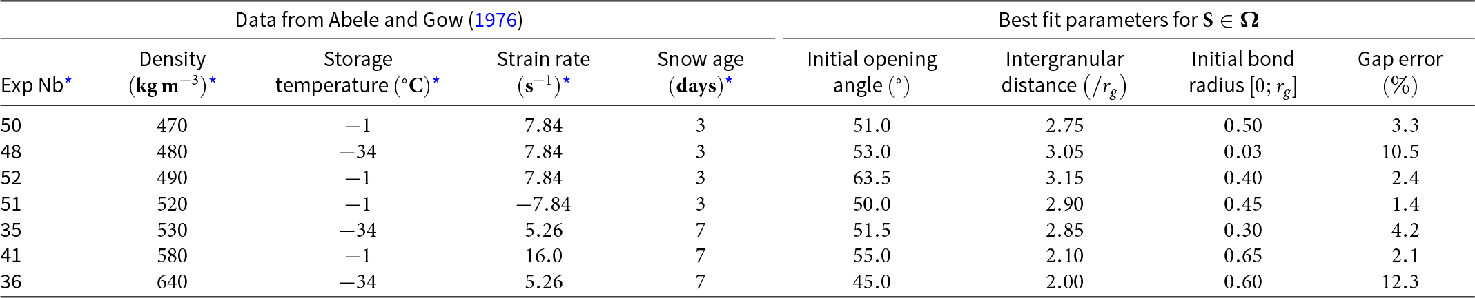
* Data from Abele and Gow (Reference Abele and Gow1976) experiments.
When plotted as a function of the initial snow density in Fig. 7, the error is found smaller in the middle of the density range. In any case, the value of the relative error between experimental and numerical curves remains relatively small, which confirms the ability of the 3-D H-model to be used as a constitutive model for snow, at least within the density range  $\left[ {470;{ }640} \right]{\text{ kg}}/{{\text{m}}^3}$. Higher densities are impossible to reach with the 3-D H-model, as the condition ${\alpha _0} = 45^\circ $ and ${d_{2,0}}/{r_{\text{g}}} = 2$ corresponds to the limit case where a contact between the two hexagons within a cell is created. For lower densities, the mismatch between experimental and numerical curves becomes too large to include these densities in the range of validity of the snow-H-model.
This first calibration was carried out blindly, in the sense that only the minimization of the gap between measured and predicted data was targeted, without considering the agreement between experimental density and model density, the latter being controlled by the two geometric parameters of the H-cell. This is the purpose of the next section, to achieve a much more versatile model.
4. Discussion on the model versatility
As the snow-H-model has demonstrated its ability to reproduce experimental results through parameter adjustment, the next step is to assess its predictive capability for snow behaviour under varying conditions of density, temperature and strain rate.
4.1. Relation between mesoscopic geometry and macroscopic density
Calculating the density in multi-scale models is challenging as its mesostructure only includes those elements which are actively participating in the force transmission. For instance, in the present model, the bi-hexagonal pattern is designed as the minimal structure to depict only snow grains which are part of force chains. The surrounding space includes both void and snow grains not participating to force transmission. This is the reason why we cannot and should not calibrate the H-cell geometry to match directly the macroscopic density. Therefore, we have chosen first to calibrate the initial geometrical parameters of the cells to match the experimental stress–strain curves from Abele and Gow (Reference Abele and Gow1976). The objective of this section is to provide an estimation of the proportion of ice grains participating to force transmission by comparing the macroscopic snow density  ${\rho _{{\text{snow}}}}$ and the mesoscopic density ${\rho _{{\text{meso}}}}$.
In the snow-H-model, we selected the smallest peripheral parallelepiped volume as the H-cell volume  ${V_{{\text{meso}}}}$ (see Fig. 9). Under this assumption, the mesoscopic density can be expressed as follows:
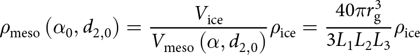 \begin{equation}{\rho _{{\text{meso}}}}\left( {{\alpha _0},{d_{2,0}}} \right) = \frac{{{V_{{\text{ice}}}}}}{{{V_{{\text{meso}}}}\left( {\alpha ,{d_{2,0}}} \right)}}{\rho _{{\text{ice}}}} = \frac{{40{{\pi }}r_{\text{g}}^3}}{{3{L_1}{L_2}{L_3}}}{\rho _{{\text{ice}}}}\end{equation}
 where  ${V_{{\text{ice}}}}$ is the volume of solid ice, which corresponds to the volume of the ten spherical grains (we neglect the ice bond volumes), and ${\rho _{{\text{ice}}}}$ is the density of ice, equal to $920{\text{ kg}}/{{\text{m}}^3}$.
The best fitting parameters obtained in Section 3.2 provide an initial density  ${\rho _{{\text{meso}}}}$ lower than 250 ${\text{kg}}\,{{\text{m}}^{ - 3}}$, while the initial densities measured in the experiments are larger than $470{\text{ kg}}/{{\text{m}}^3}$.
The density based on the bounding box shown in Fig. 8 systematically underestimates the real snow density for several reasons:
1- As already mentioned, the H-cell accounts only for grains participating in stress transmission (the force chains) whereas, in real granular materials, many grains do not transmit significant stresses. Therefore, many ice grains are not accounted for by the bi-hexagonal mesostructure, thus underestimating the solid volume.
2- The arbitrary choice for the mesoscopic volume includes much empty space and probably overestimates the void volume.
3- To a lower extent, the ideal spherical shape of the ice grain in the H-model approximates the shape of the real ice grains. In real snow, ice grains are neither spherical and nor monodisperse (see, for instance, Gay and others (Reference Gay, Fily, Genthon, Frezzotti, Oerter and Winther2002), Kaempfer and Schneebeli (Reference Kaempfer and Schneebeli2007) and Calonne and others (Reference Calonne, Flin, Geindreau, Lesaffre and du Roscoat2014)).
Gap error between experimental curves and best fitting numerical curves with initial parameters not respecting the density condition (blue crosses) and respecting the density condition presented in Section 4.1 (orange circles) as a function of the initial experimental density.
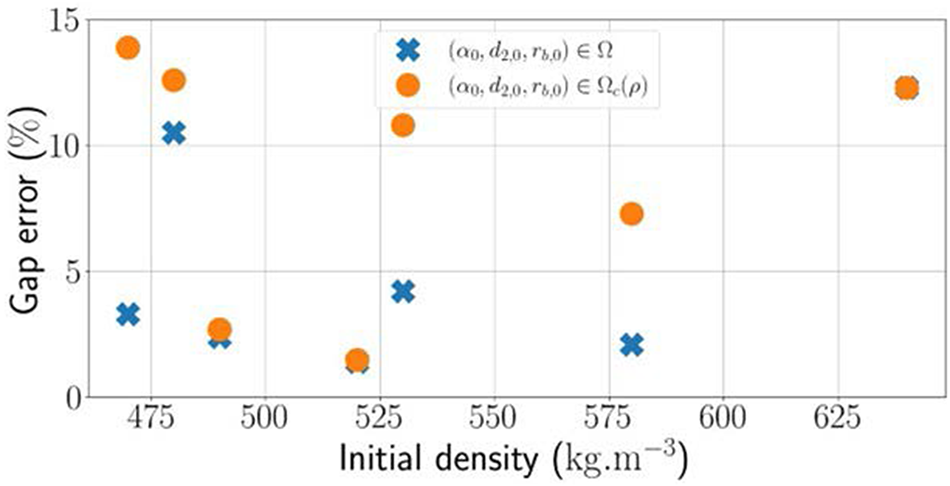
Definition of the peripheral volume of the H-cell  ${V_{{\text{meso}}}}$.

To account for the additional ice in the pore space, a coefficient γ can be introduced in the relationship between macroscopic and mesoscopic densities, as:
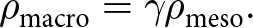 \begin{equation}{\rho _{{\text{macro}}}} = \gamma {\rho _{{\text{meso}}}}.\end{equation}
 This coefficient is set to  $\gamma = 2.58$ from the harmonic average of the ratios $\frac{{{\rho _{{\text{exp}}}}}}{{{\rho _{{\text{meso}}}}}}$ based on the calibration tests shown in Section 3 (see Table 2):
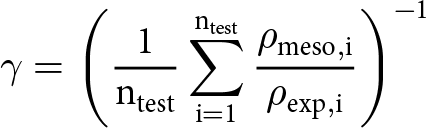 \begin{equation}{{\gamma }} = {\left( {\frac{1}{{{{\text{n}}_{{\text{test}}}}}}\mathop \sum \limits_{{\text{i}} = 1}^{{{\text{n}}_{{\text{test}}}}} \frac{{{{{\rho }}_{{\text{meso}},{\text{i}}}}{ }}}{{{{{\rho }}_{{\text{exp}},{\text{i}}}}}}} \right)^{ - 1}}{\text{ }}\end{equation}
 Figure 10 displays the analytical expression of the macroscopic density with  $\gamma = 2.58$, as a function of the opening angle for different intergranular distances, with each test used in previous Section 3.2 corresponding to a marker. The relative error is less than 2% for each test.
Density as a function of the opening angle for different initial intergranular distance  ${d_2}$. Lines represent the analytical expression of the macroscopic density with $\gamma = 2.58$. Each symbol represents a simulation, where the y-coordinate is the snow density of the corresponding experimental tests.
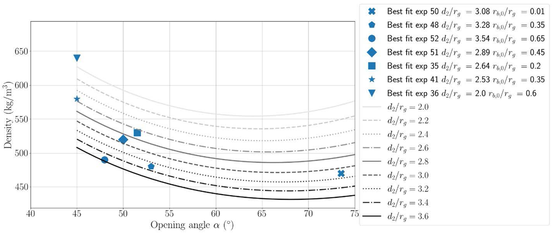
The high value of  $\gamma $ (with respect to 1) confirms that a considerable percentage of ice material is not accounted for in the density calculation. Specifically, $\gamma = 2.58$ implies that the H-cells account for $38\% $ of the mass of the material. This order of magnitude almost aligns with the observations by Wautier and others (Reference Wautier, Bonelli and Nicot2017) that the fraction of grains contributing to force chains ranges between $23\% $ and $31\% $ in sand.
In contrast to Section 3.2, the fitting procedure can be optimized by adding the additional constraint that the model density matches the experimental one. Thus, for each test  ${\text{i}}$, the best fitting triplet of initial geometrical parameters that satisfies ${\rho _{{\text{macro}}}}\left( {{\alpha _0},{d_{2,0}}} \right) = {\rho _{{\text{exp}},{\text{i}}}}$ can be searched in ${{{\Omega }}_{\text{c}}}\left( \rho \right)$ defined by:
 \begin{equation}{{{\Omega }}_{\text{c}}}\left( \rho \right) = \left\{ {\left( {{\alpha _0},{d_{2,0}},{r_{{\text{b}},0}}} \right) \in {{\Omega }}|{\rho _{{\text{macro}}}}\left( {{\alpha _0},{d_{2,0}}} \right) = \rho } \right\}\end{equation}
 The best fitting parameters accounting for the density relationship for each test are summarized in Table 3 and the corresponding stress–strain curves are plotted in Fig. 11. The maximum relative error observed is of  $13.9{\text{\% }}$, which is only slightly larger than without the constraint (39) (see Fig. 7). In general, the largest errors correspond to the extremal values of densities, while low gap errors are found for ${\rho _{{\text{exp}}}}$ close to $500{\text{ kg}}/{{\text{m}}^3}$. The discrepancy between experimental and numerical curves is maximal for small and large deformations. At small deformation, an obvious inflexion point is observed in numerical curves at the transition between elastic and plastic regimes, due to the breakage of ice bonds. Indeed, as all bridges share the same radius, ice bridges all break at the same time for a given direction of mesostructure. In a real snow sample, the radius of ice bridges varies, which means they do not break at the same deformation level. Consequently, a smoother transition between elastic and plastic regime is observed experimentally. For large deformation, the H-model does not account for the reorganization of the mesostructure, as the cells are deformed independently. This limitation of the model has been discussed by Deng (Reference Deng2022), who introduced a way to reinitialize mesostructure geometries to increase the domain of application.
Stress–strain curves for confined compression tests: experimental results from Abele and Gow (Reference Abele and Gow1976) and best fitting numerical curves obtained with the 3-D H-model for initial parameters verifying  ${\rho _{{\text{macro}}}}\left( {{\alpha _0},{d_{2,0}}} \right) = {\rho _{{\text{exp}}}}$.
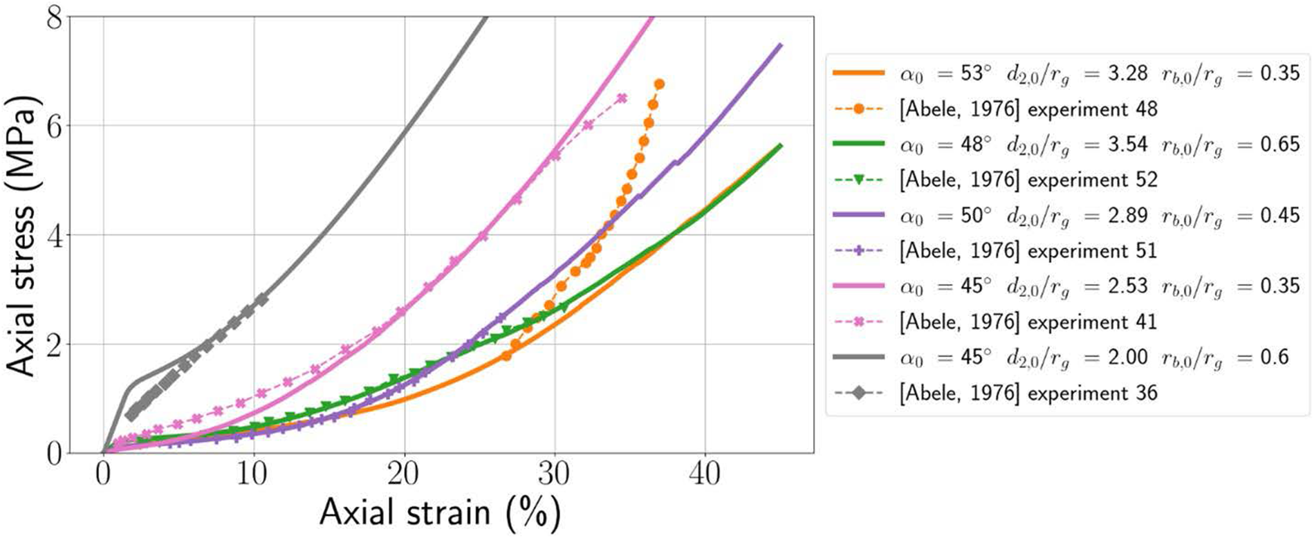
Best fitting parameters over  ${S_{bf,c}}\,$with the additional density constraint for the same experiment from Abele and Gow (Reference Abele and Gow1976) used in Section 3
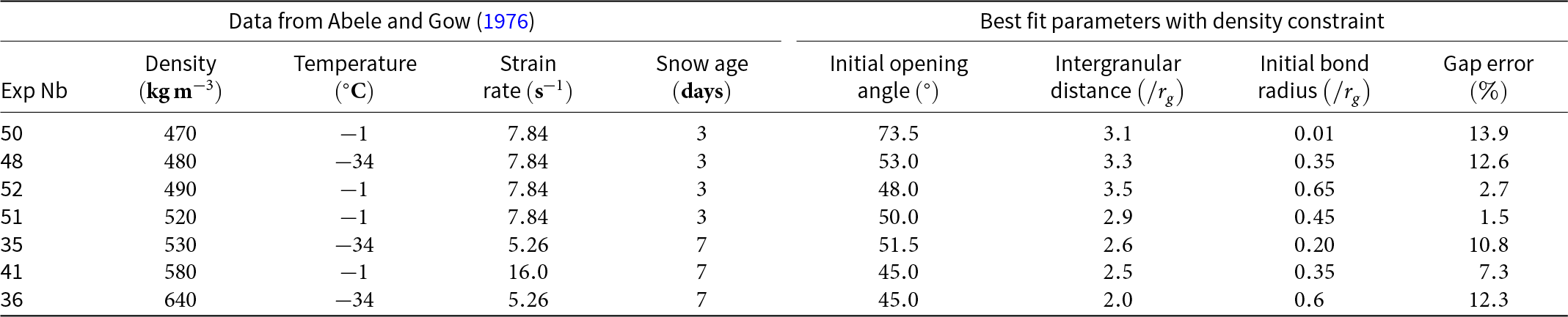
4.2. Relative influence of the three microstructure parameters on the mechanical response
Among the three parameters of the snow-H-model, two of them control the initial density (namely the initial intergranular distance  ${d_{2,0}}$ and the initial opening angle ${\alpha _0}$). The remaining parameter is the initial bond radius ${r_{{\text{b}},0}}$. It accounts for the impact of temperature and age of the snow sample. In this subsection, we characterize the relative influence of the three initial parameters of the 3-D H-model on the stress–strain curve in oedometer conditions.
1. Impact of the initial density
The initial density of a numerical snow sample is primarily determined by the geometry of the H-cells, characterized by the parameters  ${\alpha _0}$ and ${d_{2,0}}$. There is a direct relationship between ${d_2}$ and density, as the void within an H-cell increases proportionally with ${d_2}$. The stress–strain curves for a confined compression test with different initial intergranular distances ${d_{2,0}}$ are plotted in Fig. 12 (up) while the two other parameters are kept constant. Increasing the intergranular distance reduces the mesoscopic density and results in smaller axial stresses (as shown in Fig. 12 (up)), as it was observed when reducing the density of a snow sample (Landauer, Reference Landauer1955; Radke and Hobbs, Reference Radke and Hobbs1967; Abele and Gow, Reference Abele and Gow1975; Scapozza and Bartelt, Reference Scapozza and Bartelt2003; Wautier and others, Reference Wautier, Geindreau and Flin2015).
Stress–strain curves for confined compression test with different initial intergranular distances,  ${\alpha _0} = 48^\circ $ and ${r_{b,0}}/{r_g} = 0.65$ (up), and with different initial opening angles, ${d_{2,0}}/{r_g} = 3.5$ and ${r_{b,0}}/{r_g} = 0.65$ (down).
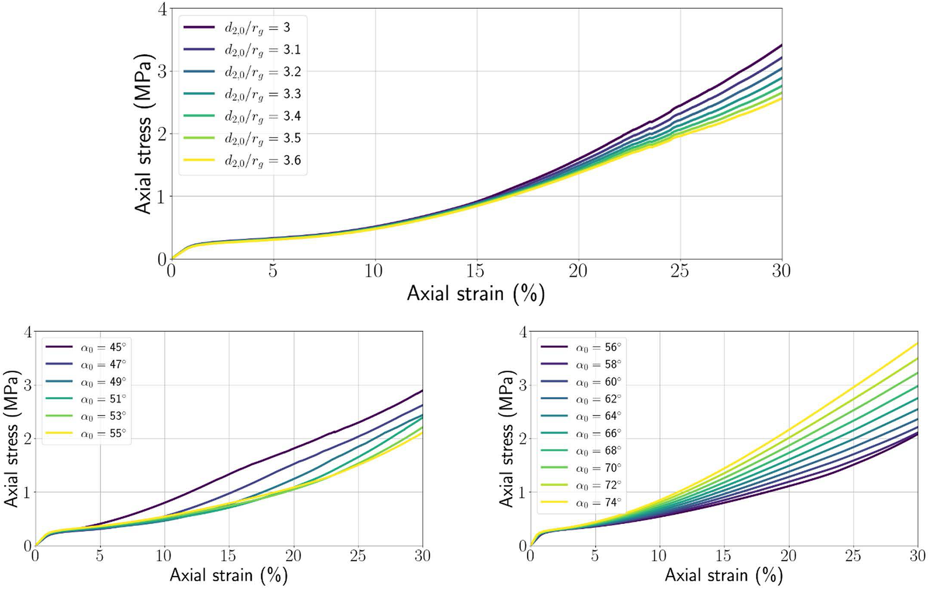
On the other hand, the relationship between the opening angle  $\alpha $ and the density is not bijective. For small values of $\alpha $, density increases with decreasing α; for larger values of $\alpha $, density increases with $\alpha $ (see Fig. 10). In Fig. 12 (down), a compression test with ${d_2}/{r_{\text{g}}} = 3.5$ and ${r_{{\text{b}},0}}/{r_{\text{g}}} = 0.65$ was run with different initial opening angles ${\alpha _0}$. The evolution of axial stress with opening angle follows the same pattern as for density. For opening angles lower than $55^\circ $, axial stress decreases when the opening angle is increased while the opposite trend is observed for opening angles larger than $55^\circ $. However, the mesoscopic density increases with the opening angle for opening angles significantly larger than $55^\circ $ (between $60^\circ $ and $70^\circ $, depending on the initial intergranular distance ${d_{2,0}}$). Thus, the non-monotonic influence of the opening angle on the stress–strain curves probably reflects the complex influence of density and other microstructural parameters (e.g. anisotropy of the contact distribution).
2. Impact of the sintering time
Another key geometrical parameter to calibrate is the initial bond radius  ${r_{{\text{b}},0}}$. While the sintering process that occurs prior to mechanical loading is not directly modelled, the initial bond radius serves as a proxy for this process since it has been shown that bond radius grows over sintering time (Kuroiwa, Reference Kuroiwa1961; Herwijnen and Miller, Reference Herwijnen and Miller2013), leading to stronger bonds (Szabo and Schneebeli, Reference Szabo and Schneebeli2007). In Fig. 13, the same compression test is now considered with different initial bond radii. It can be observed that, at the beginning of the loading, the initial bond radius has a positive effect on the axial stress. Then, as ice bonds are broken under compression, this influence of the initial bond radius is progressively reduced. It should be emphasized that the observation of enhanced stresses with the initial bond radius is somehow reminiscent to snow stiffness evolution during isothermal metamorphism (Wautier and others, Reference Wautier, Geindreau and Flin2015).
Stress–strain curves for confined compression test with different initial bond radius,  ${\alpha _0} = 48^\circ $ and ${d_{2,0}}/{r_g} = 3.5$.

Note that the growth in bond radius with sintering time cannot be readily observed from the data reported in Table 3, where the values of  ${r_{{\text{b}},0}}$ for 3 day and 7 day samples are not significantly different. This can be attributed to the fact that in the experimental work of Abele and Gow (Reference Abele and Gow1976), the snow samples were not collected immediately after a snowfall and sintering occurred prior to the sample collection. Consequently, it is difficult to link the degree of sintering solely to the storage duration.
4.3. Influence of loading conditions on the mechanical response
In this subsection, we analyse the ability of the snow-H-model to account for loading conditions that differ from those of Abele and Gow (Reference Abele and Gow1976). We focus on the strain rate and temperature influence on the mechanical response in oedometer conditions.
1. Impact of the strain rate
As the ice bonds are described by a visco-elastoplastic model, it is relevant to investigate the effect of the loading rate on the material response. As already specified, the analysis considers exclusively loading rates above  ${10^{ - 4}}{ }{{\text{s}}^{ - 1}}$ to remain within the brittle regime (Schulson, Reference Schulson2001). We can define the characteristic time ${t_{{\text{viscous}}}}$ at which the orders of magnitude of the viscoplastic and elastic deformations coincide:
 \begin{equation}{t_{{\text{viscous}}}} = \frac{{\varepsilon _{{\text{b}},{\text{n}}}^{\text{e}}}}{{A\left( {{T_{{\text{emp}}}}} \right)\sigma _{{\text{b}},{\text{n}}}^m}} \approx \frac{{{\sigma _{{\text{bcs}}}}}}{{{E_{{\text{oedo}}}}A\left( {{T_{{\text{emp}}}}} \right)\sigma _{{\text{bcs}}}^m}}\end{equation}
 where  ${\sigma _{{\text{bcs}}}}$ is the brittle compression strength of ice. At $ - {10^ \circ }{\text{C}}$, Eqn (38) gives ${t_{{\text{viscous}}}} = 24{\text{ s}}$ with ${E_{{\text{oedo}}}} = 1.6\,{\text{GPa}}$ the calibrated value of oedometer coefficient, and ${\sigma _{{\text{bcs}}}} = 13.75\,{\text{MPa}}$ from Eqn (27)
In the experiment by Abele and Gow (Reference Abele and Gow1976), the strain rates ranged between  $5{ }{{\text{s}}^{ - 1}}$ and $16{ }{{\text{s}}^{ - 1}}$, resulting in a total loading time less than $0.08{\text{ s}}$, thus much smaller than ${t_{{\text{viscous}}}}$. Consequently, for such high strain rates, the effects of viscosity can be considered negligible.
The stress–strain curves of confined compression tests performed with different strain rates on similar numerical snow samples ( ${\alpha _0} = 48^\circ $, ${r_{{\text{b}},0}} = 0.6{r_{\text{g}}}$, ${d_{2,0}} = 3.54{r_{\text{g}}}$) are given in Fig. 14. To measure the direct influence of viscosity, these curves are compared with a snow model with nonviscous bonds. The evolution of the percentage of broken bonds during the loading for the different strain rates is reported in Fig. 14. The axial stress increases with the strain rate up to $\dot \varepsilon = 0.025{ }{{\text{s}}^{ - 1}}$. For higher values, the strain rate has no significant influence on the stress–strain response which is the same as the response of the nonviscous model. This is consistent with the fact that the characteristic time of the viscous deformation ${t_{{\text{viscous}}}}$ is larger than the time needed to break the bonds at high strain rates: for example, with $\dot \varepsilon = 0.01{ }{{\text{s}}^{ - 1}}$, more than 70% of the bonds are broken after only $3\,{\text{s}}$, as shown in Fig. 14. The proportion of broken bonds increases with the strain rate (Schulson, Reference Schulson2001), as the loading rate controls the stress evolution within the bond through Glen’s law (Eqn (19)). As the contact between unbonded grains is assumed to be rate-independent in the proposed model, the strain rate effect decreases as the number of bond breakage rises, bringing the curves to converge at high strain rates. It is worth noting that at the lowest strain rates considered, the test duration could allow for the formation of additional bonds at the new contact points (see Appendix C). While the current model does not account for the formation of these new bonds, their inclusion would probably result in a more significant impact of viscosity at low strain rates.
Stress–strain curves (left) and evolution of the proportion of broken bonds (right) for confined compression tests at different strain rates, compared with a snow material with nonviscous bonds.
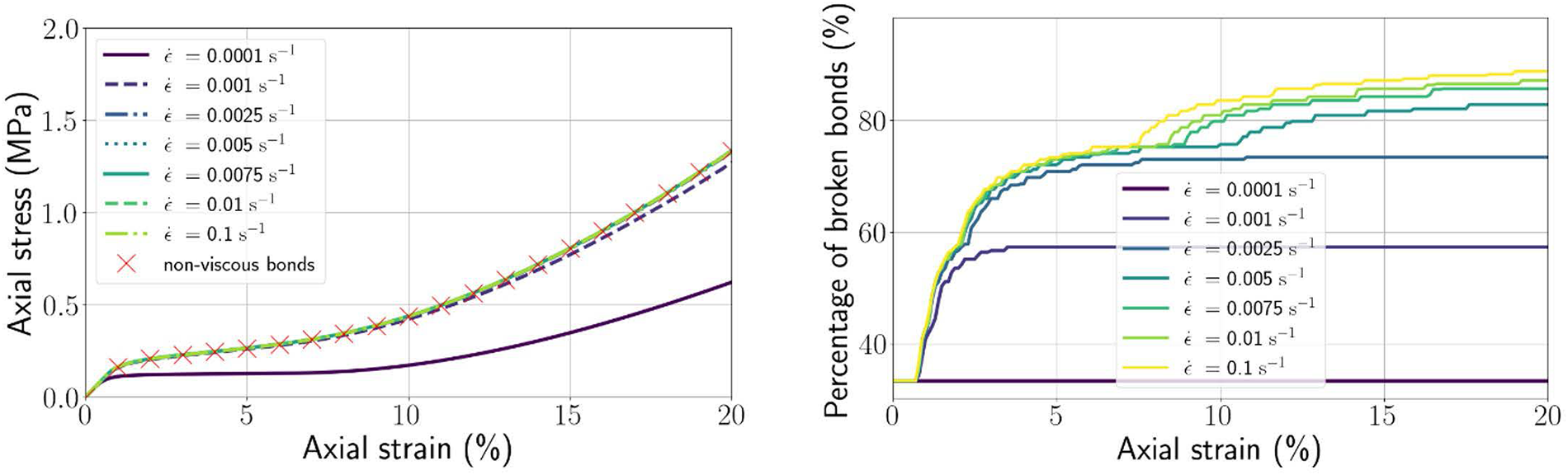
2. Impact of the temperature
The second loading parameter to studied is the temperature. McClung (Reference McClung1996), Schweizer (Reference Schweizer1998) and Takei and Maeno (Reference Takei and Maeno2004) all observed that an increase in temperature leads to a decrease in snow strength and stiffness. The temperature affects the snow mechanical behaviour independently during the sintering phase and the loading phase.
During the sintering phase, it was shown that a higher temperature leads to a higher bond growth rate (Blackford, Reference Blackford2007; Herwijnen and Miller, Reference Herwijnen and Miller2013) resulting in a greater sintering force and to an increase in the bond radius (Szabo and Schneebeli, Reference Szabo and Schneebeli2007; Bahaloo, Reference Bahaloo2022). As the snow-H-model does not model the sintering phase, the effect of the temperature during sintering cannot be assessed. However, the initial bond radius can be used as a proxy. We deduce from Fig. 13 that we have an increase of the stress with the temperature during the sintering time.
During the mechanical loading, the temperature influences both the brittle compression strength of ice defined by Eqn (28) (Schulson, Reference Schulson2001) and the viscous behaviour of the ice bonds through Glen’s law (Eqn (19)).
To measure the influence of the temperature in the model, isotropic compression tests were simulated from the same numerical snow sample ( ${\alpha _0} = 48^\circ $, ${r_{{\text{b}},0}} = 0.6{r_{\text{g}}}$, ${d_{2,0}} = 3.54{r_{\text{g}}}$) with a strain rate of $\dot \varepsilon = 7.84{ }{{\text{s}}^{ - 1}}$ at different temperatures (Fig. 15). It can be consistently observed that, for a given axial strain, the axial stresses are larger for lower temperatures, as bond failure occurs earlier in warmer conditions, as illustrated in Fig. 15 and described in Schulson (Reference Schulson1990).
Stress–strain curves (left) and evolution of the proportion of broken bonds (right) for confined compression tests at different temperatures and for  $\dot \varepsilon = 7.84\;{{\text{s}}^{ - 1}}$.
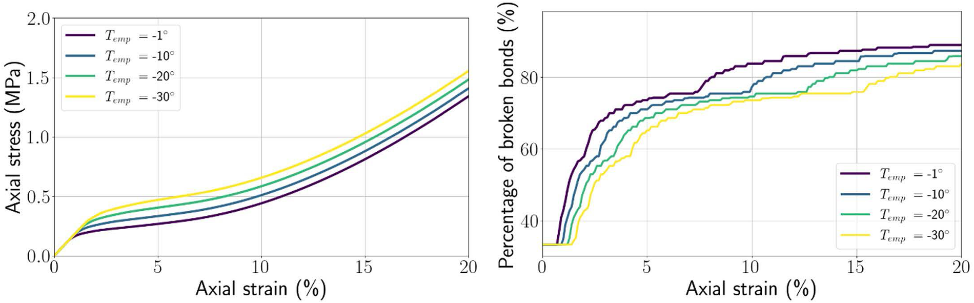
Finally, Fig. 16 shows the stress–strain curves for different temperatures with a strain rate of  $7.84{ }{{\text{s}}^{ - 1}}$, $0.001{ }{{\text{s}}^{ - 1}}$ and $0.0001{ }{{\text{s}}^{ - 1}}$. The strain rate has no significant effect for temperatures strictly below $ - 10^\circ {\text{C}}$. At higher temperatures, namely ${T_{{\text{emp}}}} = - 1^\circ {\text{C}}$ and ${T_{{\text{emp}}}} = { } - {10^ \circ }{\text{C}}$, the effect of the strain rate becomes apparent. This stems from the temperature dependent coefficient $A\left( {{T_{{\text{emp}}}}} \right)$ in Glen’s law (Eqn (19)). As this coefficient increases with temperature, the characteristic time of the viscous deformation evolves inversely with temperature. As previously mentioned, the discrepancy between the curves at ${T_{{\text{emp}}}} = - 1^\circ {\text{C}}$ and ${T_{{\text{emp}}}} = - 10^\circ {\text{C}}$ is larger at the lowest strain rate, as the effect of loading rate on ice behaviour is more marked.
Stress–strain curves for confined compression tests at different temperatures and strain rates.
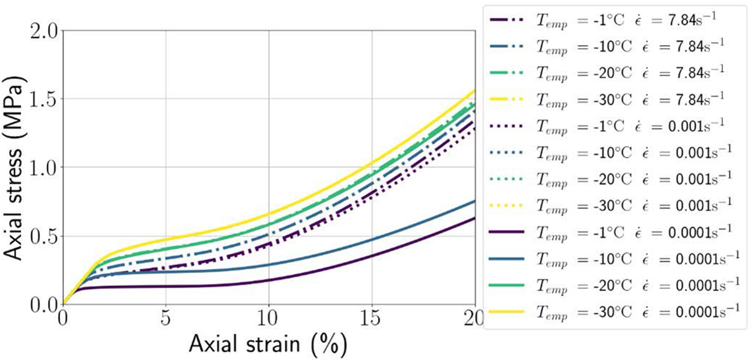
From Figs. 15 and 16, we can conclude that, for a given axial strain, the axial stress increases with decreasing temperature, whereas the snow stiffness is not affected by temperature. However, the expected influence of temperature on snow stiffness could be reproduced by considering in the model the known temperature-dependency of ice stiffness (Parameswaran, Reference Parameswaran1987).
5. Conclusions and perspectives
The 3-D H-model has been extended to snow by adding an ice bond component to the usual frictional contact law. A series of confined compression tests have been performed from numerical snow samples. The axial stress results have been compared against the experimental curves of Abele and Gow (Reference Abele and Gow1976). The ability of the snow-H-model to reproduce the mechanical behaviour of snow has been demonstrated for the intermediate range of snow density  $\left[ {470;{ }640} \right]{\text{ kg}}/{{\text{m}}^3}$, at different temperature and strain rates. For snow of lower or larger density, the calibration of the model is no longer adequate as, constitutively, the snow H-model is only able to represent the snow microstructure of intermediate density. To describe both loose and dense snow specimens, the H-cell geometry would need further adaptations. For example, changing the number of grains in the H-cell could allow to reach higher or lower density. It is worth noting that within the considered density range, the assumption of no rotation of the ice grains is reasonable, as increasing the material density enhances the connectivity between grains.
Within the domain of validity of the snow-H-model, the relationship between the geometrical parameters of the H-cell and the macroscopic density has been studied closely. Indeed, the statistical nature of the 3-D H-model prevents the pore space between the different H-cells from being accounted for. Consequently, the relationship between the mesoscopic and the macroscopic densities was derived using a proportionality coefficient. This coefficient accounts for the ice fraction that does not contribute to the loadbearing capacity of snow (i.e. the ice grains not participating to the force chains) and the void in between the H-cells.
After calibration of the model against the experimental work of Abele and Gow (Reference Abele and Gow1976), the effect of the initial bond radius has been investigated, revealing that a change in the initial bond radius produces a phenomenological response similar to what would be observed with a change in the aging time of a sample under isothermal conditions.
Finally, the impact of the loading conditions (strain rate and temperature) on the response of the snow-H-model has been highlighted. It has been shown that the strain rate (when sufficiently low) directs a substantial effect on both the viscous response of the bonds and the bond failure rate. Increasing temperature also leads to faster bond failure and smaller stresses in the material. It should be noted that the influence of strain rate on the stress–strain response is greater at higher temperatures.
As the capacity of the snow-H-model to reproduce experimental oedometer test has been proven, the next step will consist in studying the predictive ability of the model. This would require additional experiments using snow sample with a better control of the initial microstructure, and a larger range of loading condition, with lower strain rates. An implementation of the extended version of the 3-D H-model in a computational software suitable for dealing with practical engineering concerns is also considered. Using such a multi-scale approach ranging from the particle to the continuum scale is thought to bridge the gap between engineering-scale systems and the microscopic features of snow. Comparing the H-model with DEM simulations at a smaller intermediate scale would help assess computational efficiency and accuracy for snow model, as has been already demonstrated for sand on large geotechnical systems involving scales beyond the reach of DEM simulations (Xiong and others, Reference Xiong, Yin and Nicot2019).
The multi-scale approach of the model can allow to study the effect of snow microstructure in more detail. Here, the effects of the microparameters related to the snow density have been widely study, but it would be also possible to study the effect of anisotropy. All the simulations in this paper have been realized with an isotropic distribution of direction, but it would be possible to include anisotropy by modifying the probability distribution function  $\omega \left( {\theta ,\varphi ,\psi } \right)$.
New extensions of the snow-H-model can also be considered in the future. Ice bond creation and ductile failure could be added in the model, to extend the range of applicability of the model to lower strain rate. Such an improvement would made it possible to consider, for example, avalanche problems and to cover more domains application of snow mechanics.
Acknowledgements
This work was supported by the Luxembourg National Research Found FNR (SNOWTEC, project ref. 16241613).
A CC-BY public copyright license has been applied by the authors to the present document and will be applied to all subsequent versions up to the Author Accepted Manuscript arising from this submission, in accordance with the grant’s open access conditions.
The authors would like to thank the anonymous reviewers for their deep reviews of the manuscript. We sincerely appreciate the intensive work done, which helped us improve the quality of the manuscript.
Competing interests
The authors declare no competing interests.
Appendices
A Expression of the tangential force in a bonded contact between ice grain
The total shear strain  $\varepsilon _{{\text{b}},{\text{s}}}^{{\text{tot}}}$ in the bond can be split into an elastic part $\varepsilon _{{\text{b}},{\text{s}}}^{\text{e}}$ and a viscoplastic part $\varepsilon _{{\text{b}},{\text{s}}}^{{\text{vp}}}$:
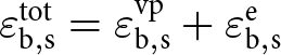 \begin{equation}\varepsilon _{{\text{b}},{\text{s}}}^{{\text{tot}}} = \varepsilon _{{\text{b}},{\text{s}}}^{{\text{vp}}} + \varepsilon _{{\text{b}},{\text{s}}}^{\text{e}}\end{equation}
 The viscoplastic deformation accounts for the creep behaviour of ice. Then, we assume that the superposition principle is applicable in Glen’s law, as it has been done in Kabore and others (Reference Kabore, Peters, Michael and Nicot2021). This assumption enables us to express the normal and shear viscous strain independently. The normal creep rate is given as a function of the normal stress with the standard expression of Eqn (19) (Barnes and others, Reference Barnes, Tabor and Walker1971). Then, for the viscous shear strain  $\dot \varepsilon _{{\text{b}},{\text{s}}}^{{\text{vp}}}$, we can write:
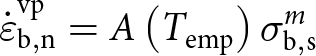 \begin{equation}\dot \varepsilon _{{\text{b}},{\text{n}}}^{{\text{vp}}} = A\left( {{T_{{\text{emp}}}}} \right)\sigma _{{\text{b}},{\text{s}}}^m\end{equation}
where  $A\left( {{T_{{\text{emp}}}}} \right)$ and $m$ are the same constant as in Eqn (19) and ${\sigma _{{\text{b}},{\text{s}}}}$ is the shear stress in the bond.
In addition, the elastic shear deformation is linearly related to the shear stress
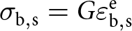 \begin{equation}{\sigma _{{\text{b}},{\text{s}}}} = G\varepsilon _{{\text{b}},{\text{s}}}^{\text{e}}\end{equation}
with  $G{ }$ the shear modulus of ice.
This gives the total viscous strain as a function of the shear stress:
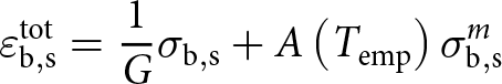 \begin{equation}\varepsilon _{{\text{b}},{\text{s}}}^{{\text{tot}}} = \frac{1}{G}{{{\sigma }}_{{\text{b}},{\text{s}}}} + A\left( {{T_{{\text{emp}}}}} \right)\sigma _{{\text{b}},{\text{s}}}^m\end{equation}
Going back to the beam representation of the ice bond in the H-cell, we can express the shear strain in the bond as:
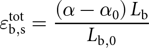 \begin{equation}\varepsilon _{{\text{b}},{\text{s}}}^{{\text{tot}}} = \frac{{\left( {\alpha - {\alpha _0}} \right){L_{\text{b}}}}}{{{L_{{\text{b}},0}}}}\end{equation}
with  $({L_{\text{b}}},\alpha )$ and $\left( {{L_{{\text{b}},0}},{\alpha _0}} \right)$ being the bond length and the H-cell opening angle, respectively, at the current time and at the beginning of the loading (Kabore and others, Reference Kabore, Peters, Michael and Nicot2021) (Peters and others, Reference Peters, Kabore, Michael and Nicot2021).
And the shear stress can be related to the tangential contact force  ${T^{\text{b}}}$ as follows:
 \begin{equation}{\sigma _{{\text{b}},{\text{s}}}} = \frac{{{T^{\text{b}}}}}{{{S_{\text{b}}}}} = \frac{{{T^{\text{b}}}}}{{{{\pi }}r_{\text{b}}^2}}\end{equation}
where  ${r_{\text{b}}}$ is the cylindrical bond radius at time $t$.
$t$.
Eventually, due to ice incompressibility in the bonds, the volume of an ice bond is supposed to be constant, so we get:
 \begin{equation}{{\pi }}{r_{\text{b}}}^2{L_{\text{b}}} = {{\pi }}{r_{{\text{b}},0}}^2{L_{{\text{b}},0}}.\end{equation}
 By combining Eqns (39)–(45), the contact law relating the incremental normal contact force  ${{\delta }}{N^{\text{b}}}$ and the incremental intergranular distance ${{\delta }}d$ reads:
 \begin{equation}{{\delta }}{T^{\text{b}}} = - \frac{{T{{\delta }}d}}{{{L_{\text{b}}}}} + {{\pi }}r_{\text{b}}^2G\frac{{{L_{\text{b}}}{{\delta }}\alpha }}{{{L_{\text{b}}}\left( {{t_0}} \right)}} - {{\pi }}r_{\text{b}}^2GA\left( {{T_{{\text{emp}}}}} \right)\sigma _{{\text{b}},{\text{t}}}^m{{\delta }}t\end{equation}
B Contact stiffness after bond failure
After bond failure, we consider that the contact force is controlled by the overlapping of the two grains at contact. As the ice grains remained deformable, the contact stiffness is strongly dependent on the contact area between the two grains. The normal contact force  ${F_{n,i}}$ is linked to the normal stiffness ${k_n}$ by the relationship:
 \begin{equation}{F_{n,i}} = {k_n}\left( {2{r_g} - {d_i}} \right)\end{equation}
with  ${r_{\text{g}}}$ being the grain radius and ${d_{\text{i}}}$ the intergranular distance.
The contact force can also be written as a function of the normal contact stress  ${\sigma _{n,i}}$:
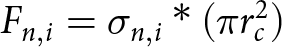 \begin{equation}{F_{n,i}} = {\sigma _{n,i}}*\left( {\pi r_c^2} \right)\end{equation}
 with  ${r_{\text{c}}} = \sqrt {r_{\text{g}}^2 - d_{\text{i}}^2/4} $ being the radius of the contact between the grain. The normal stress can be expressed in terms of normal strain ${\varepsilon _n}$:
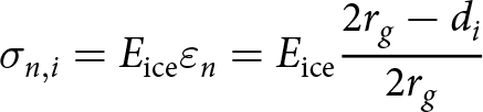 \begin{equation}{\sigma _{n,i}} = {E_{{\text{ice}}}}{\varepsilon _n} = {E_{{\text{ice}}}}\frac{{2{r_g} - {d_i}}}{{2{r_g}}}\end{equation}
So, we finally get the following expression for the normal stiffness:
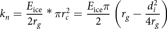 \begin{equation}{k_n} = \frac{{{E_{{\text{ice}}}}}}{{2{r_g}}}*\pi r_c^2 = \frac{{{E_{{\text{ice}}}}\pi }}{2}\left( {{r_g} - \frac{{d_i^2}}{{4{r_g}}}} \right)\end{equation}
C Creation of new contacts in the 3-D H-model H-cell
In the general case, the coordination number in a H-cell of the 3-D H-model is  $Z = 2.4$. However, depending on the loading path, the geometry of the H-cell can be deformed to a point where additional contacts are created. We can distinguish two cases: the new contact is between extremal grains 1 and 4 ( $Z = 2.6$) or between the two hexagons of the H-cell (contact between grains 2 and 7, $Z = 4$).
C-1 Creation of contact between grains 1 and 4
The contact created between grains 1 and 4 generates an additional normal contact force  ${N_5}$ to be added in the system and that contributes to the stresses in the H-cell. The value of the contact force depends on the intergranular distance ${d_5}$ between grains 1 and 4, as defined in Fig. 17 and reads:
 \begin{equation}{N_5} = - \max \left( {{k_n}\left( {2{r_g} - {d_5}} \right);0} \right)\end{equation}
Description of the creation of contact between grains 1 and 4, with  $\alpha \lt 90^\circ $: (a) scheme of one hexagon of the H-cell; (b) force equilibrium on grain 1.
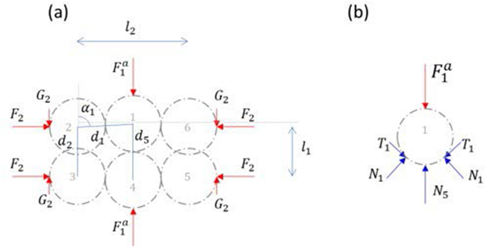
with  ${k_n}$ depending on the contact law used in the model. Adding this force does not impact the equilibrium on grain 2 and consequently does not change the way to obtain the variations of the parameters of the H-cell geometry. Only the expression of the local axial stress must be modified as follows:
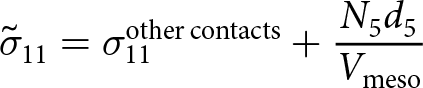 \begin{equation}{\tilde \sigma _{11}} = \sigma _{11}^{\text{other\,contacts}} + \frac{{{N_5}{d_5}}}{{{V_{\text{meso}}}}}\end{equation}
 with  $\tilde \sigma _{11}^{{\text{other contacts}}}$ the contribution of the other contact forces on the first component of the local stress tensor.
At some point, the opening angle may reach  $90^\circ $, which means that its value will not be able to increase anymore. Additional external forces must be added on grain 2 to prevent any further variation of the opening angle (see Fig. 18). In this case, the evolution of the geometry of the H-cell is directly given by ${{\delta }}{L_1}$, ${{\delta }}{L_2}$ and ${{\delta }}{L_3}$:
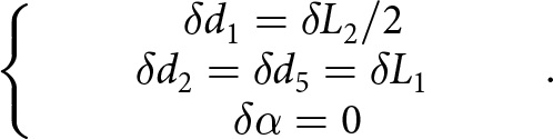 \begin{equation}\left\{ {\begin{array}{*{20}{c}}
\qquad{\delta {d_1} = \delta {L_2}/2\,\,\,\,\,\,\,\,\,} \\
{\delta {d_2} = \delta {d_5} = \delta {L_1}} \\
\qquad\qquad{\delta \alpha = 0\,\,\,\,\,\,\,\,\,\,\,\,\,\,\,\,\,\,\,\,}
\end{array}} \right..\end{equation}
\begin{equation}\left\{ {\begin{array}{*{20}{c}}
\qquad{\delta {d_1} = \delta {L_2}/2\,\,\,\,\,\,\,\,\,} \\
{\delta {d_2} = \delta {d_5} = \delta {L_1}} \\
\qquad\qquad{\delta \alpha = 0\,\,\,\,\,\,\,\,\,\,\,\,\,\,\,\,\,\,\,\,}
\end{array}} \right..\end{equation}Description of the creation of contact between grains 1 and 4, with  $\alpha = 90^\circ $: (a) scheme of one hexagon of the H-cell; (b) force equilibrium on grain 2.
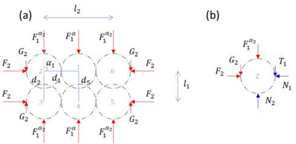
C-2 Creation of contact between the two hexagons of the same H-cell
When the lateral strains become high enough, new contacts between the two hexagons of the 3-D H-cell can appear. Considering the possibility that  ${d_2}\left( {\text{t}} \right) \ne {d_4}\left( {\text{t}} \right)$, the direction of the contact can be characterized by two Eulerian angles ${\varphi _3}$ and ${\theta _3}$ as defined in Fig. 19. ${\varphi _3}$ is the angle between the x-axis and the branch vector $\overrightarrow {{d_6}} $ between the centres of grains 2 and 7 while ${\theta _3}$ is the angle between the z-axis and the orthogonal projection of the branch vector $\overrightarrow {{d_6}} $ on the (Oyz) plane. These angles can be written:
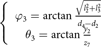 \begin{equation}\left\{ {\begin{array}{*{20}{c}}
{{\varphi _3} = \arctan \frac{{\sqrt {l_2^2 + l_3^2} }}{{{d_4} - {d_2}}}} \\
{{\theta _3} = \arctan \frac{{{y_2}}}{{{z_7}}}}
\end{array}} \right.\end{equation}
\begin{equation}\left\{ {\begin{array}{*{20}{c}}
{{\varphi _3} = \arctan \frac{{\sqrt {l_2^2 + l_3^2} }}{{{d_4} - {d_2}}}} \\
{{\theta _3} = \arctan \frac{{{y_2}}}{{{z_7}}}}
\end{array}} \right.\end{equation}Description of the creation of contact between grains 2 and 7, with  ${d_2} \ne {d_4}$: (a) scheme of the H-cell and definition of the ${\varphi _3}$ angle; (b) projection of the new contact in the plan (Oyz) and definition of the angle ${\theta _3}$.
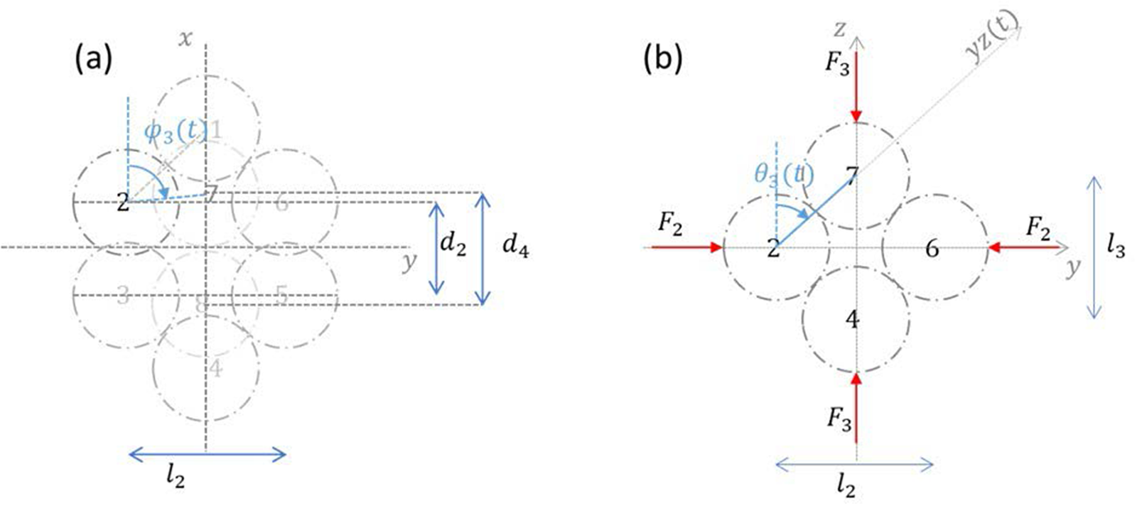
with  ${y_2}$ the y-coordinate of grain 2 and ${z_7}$ the z-coordinate of grain 7.
This new contact induces the addition of two new contact forces  ${N_6}$ and ${T_6}$ between grains 2 and 7 (see Fig. 20). The value of these forces depends on the length of the branch vector $\overrightarrow {{d_6}} $ given by the following expression:
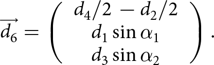 \begin{equation}\overrightarrow {{d_6}} = \left( {\begin{array}{*{20}{c}}
{{d_4}/2\, - {d_2}/2} \\
{{d_1}\sin {\alpha _1}} \\
{{d_3}\sin {\alpha _2}}
\end{array}} \right).\end{equation}
\begin{equation}\overrightarrow {{d_6}} = \left( {\begin{array}{*{20}{c}}
{{d_4}/2\, - {d_2}/2} \\
{{d_1}\sin {\alpha _1}} \\
{{d_3}\sin {\alpha _2}}
\end{array}} \right).\end{equation}Force equilibrium on grain 2: (a) in the plan (Oxy); (b) in the plan (Ozy).
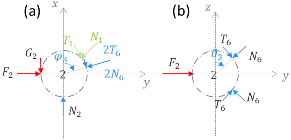
From this it follows that:
 \begin{equation}{d_6} = {\left( {{{\left( {{d_4}/2 - {d_2}/2} \right)}^2} + {{\left( {{d_1}\sin {\alpha _1}} \right)}^2} + {{\left( {{d_3}\sin {\alpha _2}} \right)}^2}} \right)^{1/2}}.\end{equation}
 The contact force  $\overrightarrow {{N_6}} { }$and the vector $\overrightarrow {{d_6}} $ being collinear, we can write:
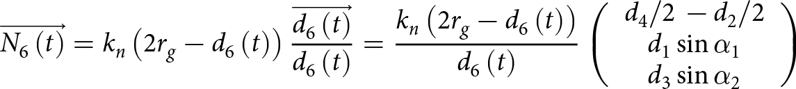 \begin{align}\overrightarrow {{N_6}\left( t \right)} = {k_n}\left( {2{r_g} - {d_6}\left( t \right)} \right)\frac{{\overrightarrow {{d_6}\left( t \right)} }}{{{d_6}\left( t \right)}} = \frac{{{k_n}\left( {2{r_g} - {d_6}\left( t \right)} \right)}}{{{d_6}\left( t \right)}}\left( {\begin{array}{*{20}{c}}
{{d_4}/2\, - {d_2}/2} \\
{{d_1}\sin {\alpha _1}} \\
{{d_3}\sin {\alpha _2}}
\end{array}} \right)\nonumber\\ \end{align}
\begin{align}\overrightarrow {{N_6}\left( t \right)} = {k_n}\left( {2{r_g} - {d_6}\left( t \right)} \right)\frac{{\overrightarrow {{d_6}\left( t \right)} }}{{{d_6}\left( t \right)}} = \frac{{{k_n}\left( {2{r_g} - {d_6}\left( t \right)} \right)}}{{{d_6}\left( t \right)}}\left( {\begin{array}{*{20}{c}}
{{d_4}/2\, - {d_2}/2} \\
{{d_1}\sin {\alpha _1}} \\
{{d_3}\sin {\alpha _2}}
\end{array}} \right)\nonumber\\ \end{align} with  ${k_n}$ depending on the contact law used in the model. In the case of a frictional law, the magnitude of the tangential contact force $\overrightarrow {{T_6}} $ reads:
 \begin{equation}\left| {{T_6}\left( t \right)} \right| = \min \left| {{T_6}\left( {t - \delta t} \right) + {k_t}{d_6}\delta {\alpha _3}} \right|,\,\left| {{N_6}\left( t \right)\tan {\varphi _g}} \right|\end{equation}
 where  ${{\delta }}{\alpha _3}\left( {\text{t}} \right)$ is the angle between $\overrightarrow {{d_6}} \left( {t - {{\delta }}t} \right)$ and $\overrightarrow {{d_6}} \left( {\text{t}} \right)$, defined by:
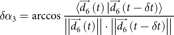 \begin{equation}\delta {\alpha _3} = \arccos \frac{\langle{\overrightarrow {{d_6}} \left( t \right){\text{|}}\overrightarrow {{d_6}} \left( {t - \delta t} \right)}\rangle}{{\left| {\left| {\overrightarrow {{d_6}} \left( t \right)} \right|} \right| \cdot \left| {\left| {\overrightarrow {{d_6}} \left( {t - \delta t} \right)} \right|} \right|\,}}\end{equation}
 The tangential contact force  $\overrightarrow {{T_6}} \left( t \right)$ is orthogonal to the normal contact force $\overrightarrow {{N_6}} \left( t \right)$ and coplanar with $\overrightarrow {{N_6}} \left( t \right)$ and $\overrightarrow {{N_6}} \left( {t - {{\delta }}t} \right)$, which means that it verifies:
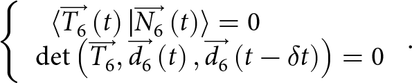 \begin{equation}\left\{ {\begin{array}{*{20}{c}}
{\langle\overrightarrow {{T_6}} \left( t \right){\text{|}}\overrightarrow {{N_6}} \left( t \right)\rangle = 0\,\,\,\,\,\,\,\,\,\,\,\,\,\,\,\,\,\,\,\,\,\,\,\,} \\
{\det \left( {\overrightarrow {{T_6}} ,\overrightarrow {{d_6}} \left( t \right),\overrightarrow {{d_6}} \left( {t - \delta t} \right)} \right) = 0}
\end{array}} \right..\end{equation}
\begin{equation}\left\{ {\begin{array}{*{20}{c}}
{\langle\overrightarrow {{T_6}} \left( t \right){\text{|}}\overrightarrow {{N_6}} \left( t \right)\rangle = 0\,\,\,\,\,\,\,\,\,\,\,\,\,\,\,\,\,\,\,\,\,\,\,\,} \\
{\det \left( {\overrightarrow {{T_6}} ,\overrightarrow {{d_6}} \left( t \right),\overrightarrow {{d_6}} \left( {t - \delta t} \right)} \right) = 0}
\end{array}} \right..\end{equation} So  $\overrightarrow {{T_6}} $ can be written:
 \begin{equation}\overrightarrow {{T_6}} = \left( {\begin{array}{*{20}{c}}
{{T_{6x}}} \\
{{T_{6y}}} \\
{{T_{6z}}}
\end{array}} \right)\end{equation}
\begin{equation}\overrightarrow {{T_6}} = \left( {\begin{array}{*{20}{c}}
{{T_{6x}}} \\
{{T_{6y}}} \\
{{T_{6z}}}
\end{array}} \right)\end{equation}with
 \begin{equation}\left\{ {\begin{array}{*{20}{c}}
{{T_{6x}} = {a_{tx}}{T_{6y}}\,\,\,\,\,\,\,\,\,\,\,\,\,\,\,\,\,\,\,\,\,\,\,\,\,\,\,\,\,} \\
{{T_{6y}} = \frac{{\left| {\overrightarrow {{T_6}} \left( t \right)} \right|}}{{\sqrt {1 + a_{tx}^2 + a_{ty}^2/a_{tz}^2\,} }}} \\
{{T_{6z}} = \frac{{{a_{ty}}}}{{{a_{tz}}}}{T_{6y}}\,\,\,\,\,\,\,\,\,\,\,\,\,\,\,\,\,\,\,\,\,\,\,\,\,\,\,\,}
\end{array}} \right.\end{equation}
\begin{equation}\left\{ {\begin{array}{*{20}{c}}
{{T_{6x}} = {a_{tx}}{T_{6y}}\,\,\,\,\,\,\,\,\,\,\,\,\,\,\,\,\,\,\,\,\,\,\,\,\,\,\,\,\,} \\
{{T_{6y}} = \frac{{\left| {\overrightarrow {{T_6}} \left( t \right)} \right|}}{{\sqrt {1 + a_{tx}^2 + a_{ty}^2/a_{tz}^2\,} }}} \\
{{T_{6z}} = \frac{{{a_{ty}}}}{{{a_{tz}}}}{T_{6y}}\,\,\,\,\,\,\,\,\,\,\,\,\,\,\,\,\,\,\,\,\,\,\,\,\,\,\,\,}
\end{array}} \right.\end{equation}and
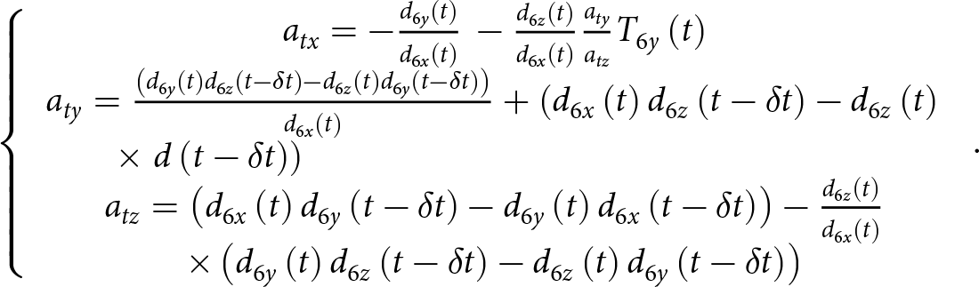 \begin{align}\left\{ {\begin{array}{*{20}{c}}
{{a_{tx}} = - \frac{{{d_{6y}}\left( t \right)}}{{{d_{6x}}\left( t \right)}}\, - \frac{{{d_{6z}}\left( t \right)}}{{{d_{6x}}\left( t \right)}}\frac{{{a_{ty}}}}{{{a_{tz}}}}{T_{6y}}\left( t \right)} \\
{a_{ty}} = \frac{{\left( {{d_{6y}}\left( t \right){d_{6z}}\left( {t - \delta t} \right) - {d_{6z}}\left( t \right){d_{6y}}\left( {t - \delta t} \right)} \right)}}{{{d_{6x}}\left( t \right)}} + \left( {d_{6x}}\left( t \right){d_{6z}}\left( {t - \delta t} \right) - {d_{6z}}\left( t \right)\right.\\ \times\left. d\left( {t - \delta t} \right) \right)\qquad\qquad\qquad\qquad\qquad\qquad\qquad\qquad{} \\
{a_{tz}} = \left( {{d_{6x}}\left( t \right){d_{6y}}\left( {t - \delta t} \right) - {d_{6y}}\left( t \right){d_{6x}}\left( {t - \delta t} \right)} \right) - \frac{{{d_{6z}}\left( t \right)}}{{{d_{6x}}\left( t \right)}}\\\times\left({d_{6y}}\left( t \right){d_{6z}}\left( {t - \delta t} \right) - {d_{6z}}\left( t \right){d_{6y}}\left( {t - \delta t} \right) \right)
\end{array}} \right..\nonumber\\ \end{align}
\begin{align}\left\{ {\begin{array}{*{20}{c}}
{{a_{tx}} = - \frac{{{d_{6y}}\left( t \right)}}{{{d_{6x}}\left( t \right)}}\, - \frac{{{d_{6z}}\left( t \right)}}{{{d_{6x}}\left( t \right)}}\frac{{{a_{ty}}}}{{{a_{tz}}}}{T_{6y}}\left( t \right)} \\
{a_{ty}} = \frac{{\left( {{d_{6y}}\left( t \right){d_{6z}}\left( {t - \delta t} \right) - {d_{6z}}\left( t \right){d_{6y}}\left( {t - \delta t} \right)} \right)}}{{{d_{6x}}\left( t \right)}} + \left( {d_{6x}}\left( t \right){d_{6z}}\left( {t - \delta t} \right) - {d_{6z}}\left( t \right)\right.\\ \times\left. d\left( {t - \delta t} \right) \right)\qquad\qquad\qquad\qquad\qquad\qquad\qquad\qquad{} \\
{a_{tz}} = \left( {{d_{6x}}\left( t \right){d_{6y}}\left( {t - \delta t} \right) - {d_{6y}}\left( t \right){d_{6x}}\left( {t - \delta t} \right)} \right) - \frac{{{d_{6z}}\left( t \right)}}{{{d_{6x}}\left( t \right)}}\\\times\left({d_{6y}}\left( t \right){d_{6z}}\left( {t - \delta t} \right) - {d_{6z}}\left( t \right){d_{6y}}\left( {t - \delta t} \right) \right)
\end{array}} \right..\nonumber\\ \end{align} For the sake of simplicity and to keep the scheme of the H-model explicit, we do not account for the influence of  $\overrightarrow {{N_6}} $ and $\overrightarrow {{T_6}} $ on the force equilibrium on grain 2, which means that the new forces only contribute to the expression of the stresses in the H-cell as follows:
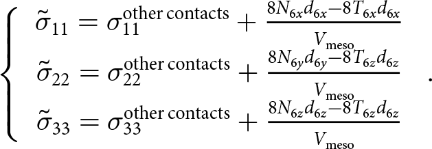 \begin{equation}\left\{ {\begin{array}{*{20}{c}}
{{{\tilde \sigma }_{11}} = \sigma _{11}^{\text{other\,contacts}} + \frac{{8{N_{6x}}{d_{6x}} - 8{T_{6x}}{d_{6x}}}}{{{V_{\text{meso}}}}}} \\[3pt]
{{{\tilde \sigma }_{22}} = \sigma _{22}^{\text{other\,contacts}} + \frac{{8{N_{6y}}{d_{6y}} - 8{T_{6z}}{d_{6z}}}}{{{V_{\text{meso}}}}}} \\[3pt]
{{{\tilde \sigma }_{33}} = \sigma _{33}^{\text{other\,contacts}} + \frac{{8{N_{6z}}{d_{6z}} - 8{T_{6z}}{d_{6z}}}}{{{V_{\text{meso}}}}}}
\end{array}} \right..\end{equation}
\begin{equation}\left\{ {\begin{array}{*{20}{c}}
{{{\tilde \sigma }_{11}} = \sigma _{11}^{\text{other\,contacts}} + \frac{{8{N_{6x}}{d_{6x}} - 8{T_{6x}}{d_{6x}}}}{{{V_{\text{meso}}}}}} \\[3pt]
{{{\tilde \sigma }_{22}} = \sigma _{22}^{\text{other\,contacts}} + \frac{{8{N_{6y}}{d_{6y}} - 8{T_{6z}}{d_{6z}}}}{{{V_{\text{meso}}}}}} \\[3pt]
{{{\tilde \sigma }_{33}} = \sigma _{33}^{\text{other\,contacts}} + \frac{{8{N_{6z}}{d_{6z}} - 8{T_{6z}}{d_{6z}}}}{{{V_{\text{meso}}}}}}
\end{array}} \right..\end{equation}D Contact loss in the 3-D H-cell
Depending on the load path of a mesostructure, some contacts between grains in a H-cell can be lost. In the case of an unbonded contact, it means that  ${d_{\text{i}}} \gt 2{r_{\text{g}}}$. In the case of a bonded contact, it occurs when the bond fails. We can distinguish two situations, depending on which contact is lost (Fig. 21). For the sake of simplicity, we consider in the following only one hexagon independently of the second one.
Description of the loss of contacts: (a) loss of the inclined contact between grains 1 and 2; (b) and (c) loss of the axial contact between grains 2 and 3 with (b) the description of the equilibrium on the two half cells and (c) the description of equilibrium on grains 1 and 2.
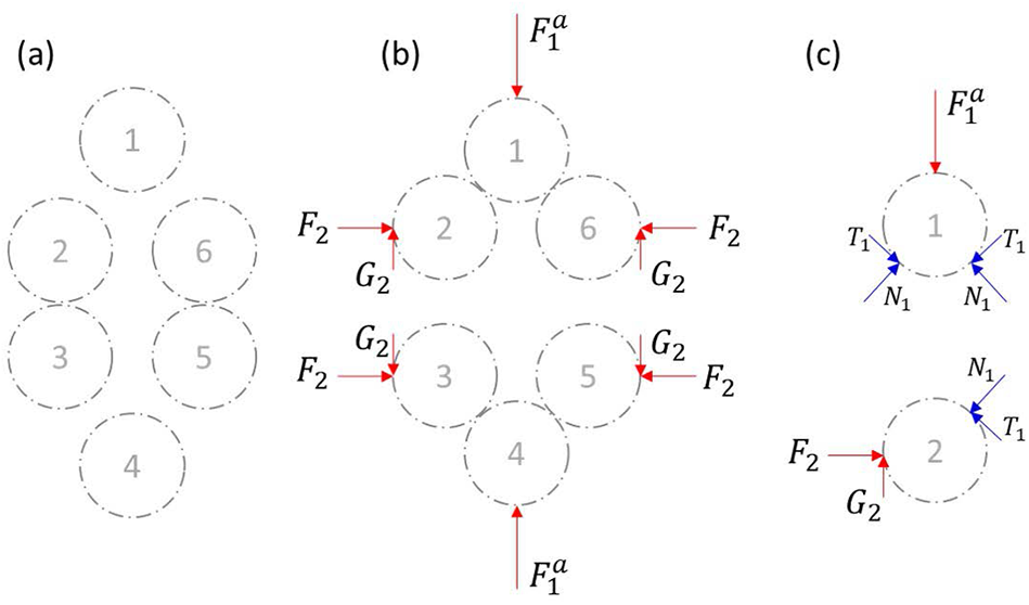
If the inclined contact (namely the one between grains 1 and 2) is lost (see Fig. 21a), the contact forces  ${N_1}$ and ${T_1}$are null, so the force equilibrium of grains 1 and 2 imposes that the external forces ${F_1}$ and ${F_2}$ are null too. The momentum equilibrium on grain 2 also imposes ${T_1} = {G_2} = 0$, which means that no force can equilibrate the normal contact force ${N_2}$ between grains 2 and 3. In that case, no force transmission is possible in the hexagon, so all the stresses are null. In this work, we have chosen to let the deformation of the cell continue until the contact is restored. We fix ${d_2} = 2{r_{\text{g}}}$, and the geometrical compatibility equations (4) and (5) enables to determine the variation of ${d_1}$ and $\alpha $.
If the axial contact between grains 2 and 3 is lost, the normal contact force  ${N_2}$ is null. In this case, one hexagon is separated into two triangles (see Fig. 21b, c). The equilibrium equation of forces and momentum on grain 2 leads to:
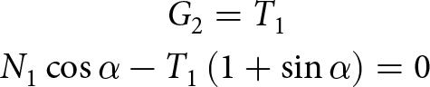 \begin{align}{G_2} = {T_1}\qquad\quad\quad \nonumber\\ {N_1} \cos \alpha - {T_1}\left( {1 + \sin \alpha } \right) = 0\end{align}
 where  ${N_1}{ }$and ${T_1}$ are of opposite signs. This means that the system to solve in this case becomes:
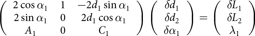 \begin{equation}\left( {\begin{array}{*{20}{c}}
{2\cos {\alpha _1}}&1&{ - 2{d_1}\sin {\alpha _1}} \\
{2\sin {\alpha _1}}&0&{2{d_1}\cos {\alpha _1}} \\
{{A_1}}&0&{{C_1}}
\end{array}} \right)\left( {\begin{array}{*{20}{c}}
{\delta {d_1}} \\
{\delta {d_2}} \\
{\delta {\alpha _1}}
\end{array}} \right) = \left( {\begin{array}{*{20}{c}}
{\delta {L_1}} \\
{\delta {L_2}} \\
{{\lambda _1}}
\end{array}} \right)\end{equation}
\begin{equation}\left( {\begin{array}{*{20}{c}}
{2\cos {\alpha _1}}&1&{ - 2{d_1}\sin {\alpha _1}} \\
{2\sin {\alpha _1}}&0&{2{d_1}\cos {\alpha _1}} \\
{{A_1}}&0&{{C_1}}
\end{array}} \right)\left( {\begin{array}{*{20}{c}}
{\delta {d_1}} \\
{\delta {d_2}} \\
{\delta {\alpha _1}}
\end{array}} \right) = \left( {\begin{array}{*{20}{c}}
{\delta {L_1}} \\
{\delta {L_2}} \\
{{\lambda _1}}
\end{array}} \right)\end{equation}with  ${A_1}$, ${C_1}$ and ${\lambda _1}$ as defined in Eqn (12), depending on the contact law.
We can calculate  $F_1^a$ from the equilibrium on the forces on grain 1 projected on the axis of the cell:
 \begin{equation}F_1^a = 2{N_1}\cos \alpha - 2{T_1}\sin \alpha \end{equation}
From Eqn (65), we deduce that:
 \begin{equation}F_1^a = 2{G_2}\end{equation}
which proves that the two half-cells are in equilibrium.
This external tangential force  ${G_2}$ represents the action of the grains outside the cell on the grain within the cell, indicating that connectivity is established through contact with neighbouring cells. As illustrated in Fig. 22, the connectivity of grains 1 and 4 in the grey cell is ensured by their contact with the blue and orange cells.
Description of the connectivity the grain in a cell with a loss of contact between grains 2 and 3 (grey cell), throughout the neighbouring cells.
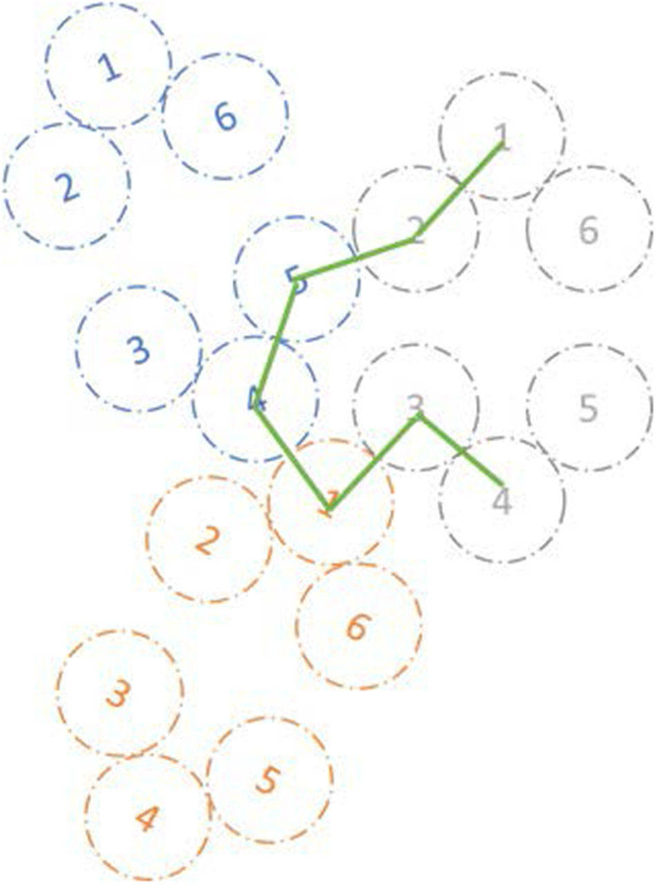


 Open access