


Impact Statement
This research addresses a current challenge in structural engineering of increasing importance: designing efficient and reliable structures in the face of uncertainty—a key consideration in reducing the carbon footprint of construction. Our framework offers a simple but effective solution to the computational challenges of reliability-based design optimization that works well in low dimensions. Since the method is agnostic to the type of numerical structural model used, the approach is applicable to many problems beyond the presented example on prestressed concrete design. Ultimately, this work contributes to the development of a more sustainable built environment by enabling more efficient use of materials while explicitly maintaining adequate safety standards.
1. Introduction
Uncertainty in the context of structural engineering exists in material properties, environmental conditions, and structural geometry, as well as within structural analysis models and as a result of human error. Ambiguity in these quantities arises from either a lack of data or due to inherent randomness (Faber and Sørensen, Reference Faber and Sørensen2002). Modern building codes, such as the Eurocodes (CEN, 2002), deal with uncertainties in design by adopting a load and resistance factor approach, first introduced by Ellingwood in the early 1980s (Ellingwood et al., Reference Ellingwood, MacGregor, Galambos and Cornell1982), which applies factors of safety (termed partial safety factors) to both loads and resistances. While modern codes have been highly successful in delivering high standards of safety and performance in design, they possess a number of limitations. Partial safety factors are deterministic and only implicitly account for the probabilistic nature of loads and material strengths. In applying partial safety factors uniformly across a wide range of structure types and construction practices, it is likely that there exists over-conservatism in design in some scenarios and under-conservatism in others. Structural engineering as a profession has accumulated a wealth of implicit knowledge based on historic trial and error. This has helped form the basis of the calibration of code partial safety factors (Faber and Sørensen, Reference Faber and Sørensen2002), which are to some extent subjective. In light of climate goals, it may be warranted to reconsider the trade-offs between safety and efficiency in design.
One approach to design structures whilst explicitly accounting for uncertainty is reliability-based design optimization (Hu et al., Reference Hu, Cheng, Yan, Cheng, Peng, Cho and Lee2024). In contrast to deterministic optimization, which assumes fixed values for parameters, reliability-based optimization accounts for variability in inputs. Specifically, probabilistic constraints (also known as chance constraints) are used to ensure the design achieves a desired level of reliability. Reliability-based optimization problems are difficult to solve: they are generally non-convex, even if the underlying functions in the constraint and objective are convex, and hence it cannot be guaranteed that a local minimum is the global optimum (Campi and Garatti, Reference Campi and Garatti2011). In addition, checking the feasibility of objectives and constraints is computationally expensive because it requires multivariate integration, which is an NP-hard problem (Khachiyan, Reference Khachiyan1989). Classical methods used to solve reliability-based optimization within the discipline of engineering have been developed extensively since the 1960s (Hilton and Feigen, Reference Hilton and Feigen1960). These methods typically rely on deterministic approximations to evaluate system reliability and struggle to model complex, highly nonlinear systems. Whilst simulation-based approaches (such as Monte Carlo simulation) alleviate this issue, they can be prohibitively expensive where computationally demanding numerical models define the optimization objective or constraints. To address these challenges, machine learning surrogate modeling—where a sample-efficient model trained on data replaces the expensive simulation—has emerged as a powerful tool for simulation-based reliability assessment (Moustapha and Sudret, Reference Moustapha and Sudret2019). The use of these surrogate models, however, can still require numerous simulations to generate training data. Consequently, a number of studies have explored using Bayesian optimization, which strategically selects training points to minimize the number of model evaluations needed, to optimize engineering systems under uncertainty with minimal computational cost.
In this paper, we focus on reliability-constrained Bayesian optimization, an extension of standard Bayesian optimization that incorporates objectives and constraints expressed probabilistically. In this framework, engineers can optimize designs while accounting for statistical uncertainty in the input parameters. We base our work upon recent advances in reliability-constrained Bayesian optimization. A number of studies have investigated this topic, either from an engineering design perspective, where it is generally referred to as robust design (Apley et al., Reference Apley, Liu and Chen2006; Arendt et al., Reference Arendt, Apley and Chen2013; Do et al., Reference Do, Ohsaki and Yamakawa2021; Zhang et al., Reference Zhang, Zhu, Chen and Arendt2013) or from a computer science perspective, where phrases such as optimization “with expensive integrands” or “of integrated response functions” are common (Groot et al., Reference Groot, Birlutiu, Heskes, Coelho, Studer and Wooldridg2010; Swersky et al., Reference Swersky, Snoek and Adams2013; Tesch et al., Reference Tesch, Schneider and Choset2011; Toscano-Palmerin and Frazier, Reference Toscano-Palmerin and Frazier2022; Williams et al., Reference Williams, Santner and Notz2000). In the former case, optimization of a statistical measure (e.g., mean, or mean and variance) of an engineering system, given varying environmental conditions, leads to a reliability-based or robust design optimization problem (Arendt et al., Reference Arendt, Apley and Chen2013; Daulton et al., Reference Daulton, Cakmak, Balandat, Osborne, Zhou and Bakshy2022; Tesch et al., Reference Tesch, Schneider and Choset2011). In the latter case, optimizing machine learning model hyperparameters across multiple tasks or cross-validation batches is mathematically similar to optimizing the expected value of a random function [in the discrete case] (Swersky et al., Reference Swersky, Snoek and Adams2013; Toscano-Palmerin and Frazier, Reference Toscano-Palmerin and Frazier2022). These approaches generally utilize modifications of well-known deterministic Bayesian optimization strategies (see Section 3).
Whilst the studies previously mentioned have effectively addressed unconstrained optimization problems under uncertainty, structural design presents unique challenges, where constraints often take precedence over objectives (Mathern et al., Reference Mathern, Steinholtz, Sjöberg, Önnheim, Ek, Rempling, Gustavsson and Jirstrand2021). Despite the importance of this field, there have been relatively few contributions specifically targeting structural design and its distinctive equations and problem formulations. To our knowledge, no previous research has investigated prestressed concrete design—a key focus of our paper. While Bayesian optimization has been applied to deterministic structural design (Mathern et al., Reference Mathern, Steinholtz, Sjöberg, Önnheim, Ek, Rempling, Gustavsson and Jirstrand2021) and in a limited number of reliability-based studies (Do et al., Reference Do, Ohsaki and Yamakawa2021), our work makes several new contributions. First, we expand the application to structural engineering examples, which remain underrepresented in the literature. Second, we implement fast, parallel batch optimization with gradient-based methods, which represents an advancement over earlier robust design approaches (Apley et al., Reference Apley, Liu and Chen2006; Arendt et al., Reference Arendt, Apley and Chen2013; Do et al., Reference Do, Ohsaki and Yamakawa2021; Zhang et al., Reference Zhang, Zhu, Chen and Arendt2013). Third, we demonstrate how Gaussian process surrogates can successfully model prestressed concrete design in the context of Bayesian optimization.
It is worth distinguishing the proposed framework from existing adaptive reliability analysis approaches (Bichon et al., Reference Bichon, Eldred, Swiler, Mahadevan and McFarland2008; Moustapha and Sudret, Reference Moustapha and Sudret2019). These methods use acquisition functions to refine a surrogate near a limit-state boundary for improved failure probability estimation, often within a double-loop optimization process. In contrast, the presented framework integrates reliability assessment within a Bayesian optimization approach: model evaluations are selected to improve the reliability-constrained objective itself, unifying reliability estimation and optimization within a single loop. While a direct quantitative comparison with FORM or SORM-based algorithms (Hu et al., Reference Hu, Cheng, Yan, Cheng, Peng, Cho and Lee2024)—classical methods of reliability-based optimization performed by approximating the limit-state surface using first or second-order expansions at the design point—is beyond the scope of this study, the presented results illustrate instead how a Bayesian approach can be applied to practical problems in structural design.
The paper is organized as follows: Section 2 outlines the proposed surrogate modeling and optimization framework; Section 3 describes our implementation; Section 4 shows the results of the method applied to both analytic test functions from the literature and an engineering example; Section 5 discusses the implications of our findings and potential limitations of the approach; and Section 6 concludes the paper with a summary of contributions and suggestions for future work.
2. Reliability-based design optimization
This study is focused on the reliability-based optimization problem described by Equation 2.1. In general, reliability-based optimization aims to maximize some statistical measure whilst ensuring satisfaction of probabilistic constraints. In our case, we maximize the expected value of the function $ f\left(\mathbf{x},\boldsymbol{\xi} \right) $
, whilst ensuring that reliability constraints
$ f\left(\mathbf{x},\boldsymbol{\xi} \right) $
, whilst ensuring that reliability constraints $ \mathrm{P}\left[{g}_i\left(\mathbf{x},\boldsymbol{\xi} \right)\le 0\right] $
are satisfied with a specified probability
$ \mathrm{P}\left[{g}_i\left(\mathbf{x},\boldsymbol{\xi} \right)\le 0\right] $
are satisfied with a specified probability $ 1-{\beta}_i $
:
$ 1-{\beta}_i $
:
 $$ \underset{\mathbf{x}\in \mathcal{X}}{\max}\hskip1em \unicode{x1D53C}\left[f\left(\mathbf{x},\boldsymbol{\xi} \right)\right] $$
 $$ \mathrm{P}\left[{g}_i\left(\mathbf{x},\boldsymbol{\xi} \right)\le 0\right]\ge 1-{\beta}_i,\hskip1em i=1,\dots, m $$
In the above Equation (2.1), $ \mathbf{x}\in \mathcal{X}\subset {\mathrm{\mathbb{R}}}^d $
are deterministic design variables, and
$ \mathbf{x}\in \mathcal{X}\subset {\mathrm{\mathbb{R}}}^d $
are deterministic design variables, and $ \boldsymbol{\xi} \in \Xi $
are uncertain parameters drawn from a probability distribution over the domain
$ \boldsymbol{\xi} \in \Xi $
are uncertain parameters drawn from a probability distribution over the domain $ \Xi $
.
$ \Xi $
. $ \unicode{x1D53C} $
and
$ \unicode{x1D53C} $
and $ \mathrm{P} $
denote an expected value and a probability, respectively. The optimization objective and constraint functions depend on the uncertain parameters but, in contrast to the design variables, they are not controlled by the optimization procedure. What we refer to as uncertain parameters are also commonly referred to as random environmental variables (Toscano-Palmerin and Frazier, Reference Toscano-Palmerin and Frazier2022), emphasizing their role as uncontrollable random variables of known distribution. In the context of structural design, the imposed (or variable) load from the occupants of a building is a good example of a random environmental variable: the number of people using a particular building cannot generally be explicitly controlled but a probability distribution representing that load can be estimated with reasonable precision.
$ \mathrm{P} $
denote an expected value and a probability, respectively. The optimization objective and constraint functions depend on the uncertain parameters but, in contrast to the design variables, they are not controlled by the optimization procedure. What we refer to as uncertain parameters are also commonly referred to as random environmental variables (Toscano-Palmerin and Frazier, Reference Toscano-Palmerin and Frazier2022), emphasizing their role as uncontrollable random variables of known distribution. In the context of structural design, the imposed (or variable) load from the occupants of a building is a good example of a random environmental variable: the number of people using a particular building cannot generally be explicitly controlled but a probability distribution representing that load can be estimated with reasonable precision.
It should be noted that alternative formulations of design optimization under uncertainty are possible where the design variables themselves are subject to noise (Zhang et al., Reference Zhang, Zhu, Chen and Arendt2013; Sui et al., Reference Sui, Gotovos, Burdick and Krause2015; Daulton et al., Reference Daulton, Cakmak, Balandat, Osborne, Zhou and Bakshy2022), that is, $ f\left(\mathbf{x}+\boldsymbol{\xi} \right) $
; however, such formulations are not the focus of this paper. In Equation 2.1, the probabilistic (or chance) constraints are assumed to be statistically independent. The case of correlated constraints, which must to satisfied jointly, represents a more complex problem (Do et al., Reference Do, Ohsaki and Yamakawa2021) and is beyond the scope of this paper.
$ f\left(\mathbf{x}+\boldsymbol{\xi} \right) $
; however, such formulations are not the focus of this paper. In Equation 2.1, the probabilistic (or chance) constraints are assumed to be statistically independent. The case of correlated constraints, which must to satisfied jointly, represents a more complex problem (Do et al., Reference Do, Ohsaki and Yamakawa2021) and is beyond the scope of this paper.
3. Bayesian optimization
Bayesian optimization (BayesOpt) is an approach to global optimization which involves two steps performed sequentially: (1) a surrogate model, based on observed data $ \mathcal{D}={\left\{\left(\left({\mathbf{x}}_i,{\boldsymbol{\xi}}_i\right),f\left({\mathbf{x}}_i,{\boldsymbol{\xi}}_i\right)\right)\right\}}_{i=1}^n $
, is created, providing a predictive distribution over unseen points; (2) heuristics (called acquisition functions) are then used to decide where to next sample additional data based on the predictive distribution of the current surrogate model. The acquisition function itself may be multimodal and hence hard to optimize, and so BayesOpt makes sense primarily in the case where the original functions being modeled are expensive or time-consuming. A simple example of BayesOpt is shown in Figure 1; an unknown objective function is sampled at points, which are then used to train a Gaussian process surrogate. The distribution in terms of mean and standard deviation of the surrogate is then used to construct an acquisition function. A tutorial on BayesOpt is provided by Frazier (Reference Frazier2018).
$ \mathcal{D}={\left\{\left(\left({\mathbf{x}}_i,{\boldsymbol{\xi}}_i\right),f\left({\mathbf{x}}_i,{\boldsymbol{\xi}}_i\right)\right)\right\}}_{i=1}^n $
, is created, providing a predictive distribution over unseen points; (2) heuristics (called acquisition functions) are then used to decide where to next sample additional data based on the predictive distribution of the current surrogate model. The acquisition function itself may be multimodal and hence hard to optimize, and so BayesOpt makes sense primarily in the case where the original functions being modeled are expensive or time-consuming. A simple example of BayesOpt is shown in Figure 1; an unknown objective function is sampled at points, which are then used to train a Gaussian process surrogate. The distribution in terms of mean and standard deviation of the surrogate is then used to construct an acquisition function. A tutorial on BayesOpt is provided by Frazier (Reference Frazier2018).
A simple illustration of Bayesian optimization. A Gaussian process model, trained on four noiseless observations, is visualized, along with the corresponding acquisition function used to select the next evaluation point.

3.1. Gaussian process
The canonical surrogate model used in BayesOpt is a Gaussian process, which is briefly described here. A Gaussian process is a collection of random variables, any finite subset of which has a joint Gaussian distribution (Rasmussen and Williams, Reference Rasmussen and Williams2006). A Gaussian process is fully specified by a mean function and covariance function, that is, $ \hat{f}\;\left(\mathbf{x}\right)\sim \mathcal{GP}\left(m\left(\mathbf{x}\right),k\left(\mathbf{x},{\mathbf{x}}^{\prime}\right)\right) $
. Note that for visual clarity, dependence on ξ has been dropped from the notation in this section; x can be taken to mean (x,ξ). In the absence of specific knowledge about the underlying trend, the mean function is set to zero, that is,
$ \hat{f}\;\left(\mathbf{x}\right)\sim \mathcal{GP}\left(m\left(\mathbf{x}\right),k\left(\mathbf{x},{\mathbf{x}}^{\prime}\right)\right) $
. Note that for visual clarity, dependence on ξ has been dropped from the notation in this section; x can be taken to mean (x,ξ). In the absence of specific knowledge about the underlying trend, the mean function is set to zero, that is, $ m\left(\mathbf{x}\right)=0 $
, which represents an uninformative prior on the function values. The covariance function
$ m\left(\mathbf{x}\right)=0 $
, which represents an uninformative prior on the function values. The covariance function $ k\left(\mathbf{x},{\mathbf{x}}^{\prime}\right) $
encodes the belief that points
$ k\left(\mathbf{x},{\mathbf{x}}^{\prime}\right) $
encodes the belief that points $ {\mathbf{x}}_i,{\mathbf{x}}_j $
that are close in the input space will have similar function values in the output space. The squared exponential covariance function is the most common and is used in this work:
$ {\mathbf{x}}_i,{\mathbf{x}}_j $
that are close in the input space will have similar function values in the output space. The squared exponential covariance function is the most common and is used in this work:
 $$ k\left(\mathbf{x},{\mathbf{x}}^{\prime}\right)={\sigma}_f^2\exp \left(-\frac{{\left|\mathbf{x}-{\mathbf{x}}^{\prime}\right|}^2}{2{\mathrm{\ell}}^2}\right) $$
which has hyperparameters $ \boldsymbol{\theta} =\left({\sigma}_f^2,\mathrm{\ell}\right) $
, obtained by maximizing the log marginal likelihood
$ \boldsymbol{\theta} =\left({\sigma}_f^2,\mathrm{\ell}\right) $
, obtained by maximizing the log marginal likelihood $ \log \mathrm{p}\left(\mathbf{y}|\mathbf{X},\boldsymbol{\theta} \right) $
. The log marginal likelihood has a well-known closed-form expression (Rasmussen and Williams, Reference Rasmussen and Williams2006). Given a set of observations
$ \log \mathrm{p}\left(\mathbf{y}|\mathbf{X},\boldsymbol{\theta} \right) $
. The log marginal likelihood has a well-known closed-form expression (Rasmussen and Williams, Reference Rasmussen and Williams2006). Given a set of observations $ \mathbf{y}={\left[{y}_1,\dots, {y}_n\right]}^{\top}\in {\mathrm{\mathbb{R}}}^n $
associated with training inputs
$ \mathbf{y}={\left[{y}_1,\dots, {y}_n\right]}^{\top}\in {\mathrm{\mathbb{R}}}^n $
associated with training inputs $ \mathbf{X}={\left[{\mathbf{x}}_1,\dots, {\mathbf{x}}_n\right]}^{\top}\in {\mathrm{\mathbb{R}}}^{n\times d} $
and a set of query points
$ \mathbf{X}={\left[{\mathbf{x}}_1,\dots, {\mathbf{x}}_n\right]}^{\top}\in {\mathrm{\mathbb{R}}}^{n\times d} $
and a set of query points $ {\mathbf{X}}^{\ast }={\left[{\mathbf{x}}_1^{\ast },\dots, {\mathbf{x}}_k^{\ast}\right]}^{\top}\in {\mathrm{\mathbb{R}}}^{k\times d} $
, Gaussian process regression provides a posterior predictive distribution
$ {\mathbf{X}}^{\ast }={\left[{\mathbf{x}}_1^{\ast },\dots, {\mathbf{x}}_k^{\ast}\right]}^{\top}\in {\mathrm{\mathbb{R}}}^{k\times d} $
, Gaussian process regression provides a posterior predictive distribution $ {\mathbf{y}}^{\ast } $
over the query points given by
$ {\mathbf{y}}^{\ast } $
over the query points given by
 $$ {\mathbf{y}}^{\ast}\mid \mathbf{X},\mathbf{y},{\mathbf{X}}^{\ast}\sim \mathcal{N}\left(\boldsymbol{\mu} \left({\mathbf{X}}^{\ast}\right),\boldsymbol{\Sigma} \left({\mathbf{X}}^{\ast}\right)\right) $$
 $$ \boldsymbol{\mu} \left({\mathbf{X}}^{\ast}\right)=K\left({\mathbf{X}}^{\ast },\mathbf{X}\right)K{\left(\mathbf{X},\mathbf{X}\right)}^{-1}\mathbf{y} $$
 $$ \boldsymbol{\Sigma} \left({\mathbf{X}}^{\ast}\right)=K\left({\mathbf{X}}^{\ast },{\mathbf{X}}^{\ast}\right)-K\left({\mathbf{X}}^{\ast },\mathbf{X}\right)K{\left(\mathbf{X},\mathbf{X}\right)}^{-1}K\left(\mathbf{X},{\mathbf{X}}^{\ast}\right) $$
where $ K\left(\mathbf{X},\mathbf{X}\right)\in {\mathrm{\mathbb{R}}}^{n\times n} $
is the covariance matrix between the previously seen points, with entries
$ K\left(\mathbf{X},\mathbf{X}\right)\in {\mathrm{\mathbb{R}}}^{n\times n} $
is the covariance matrix between the previously seen points, with entries $ {K}_{ij}=k\left({\mathbf{x}}_i,{\mathbf{x}}_j\right) $
. Similarly,
$ {K}_{ij}=k\left({\mathbf{x}}_i,{\mathbf{x}}_j\right) $
. Similarly, $ K\left({\mathbf{X}}^{\ast },{\mathbf{X}}^{\ast}\right)\in {\mathrm{\mathbb{R}}}^{k\times k} $
is the covariance matrix at the query points, and
$ K\left({\mathbf{X}}^{\ast },{\mathbf{X}}^{\ast}\right)\in {\mathrm{\mathbb{R}}}^{k\times k} $
is the covariance matrix at the query points, and $ K\left({\mathbf{X}}^{\ast },\mathbf{X}\right)\in {\mathrm{\mathbb{R}}}^{k\times n} $
is the cross-covariance matrix between the query points and the previously seen points, with entries
$ K\left({\mathbf{X}}^{\ast },\mathbf{X}\right)\in {\mathrm{\mathbb{R}}}^{k\times n} $
is the cross-covariance matrix between the query points and the previously seen points, with entries $ {K}_{ij}=k\left({\mathbf{x}}_i^{\ast },{\mathbf{x}}_j\right) $
. In essence, a Gaussian process (hereafter denoted by a hat symbol such as
$ {K}_{ij}=k\left({\mathbf{x}}_i^{\ast },{\mathbf{x}}_j\right) $
. In essence, a Gaussian process (hereafter denoted by a hat symbol such as $ \hat{f} $
) provides a prediction over unseen points
$ \hat{f} $
) provides a prediction over unseen points $ {\mathbf{x}}^{\ast} $
, represented as a Gaussian distribution with a mean and variance
$ {\mathbf{x}}^{\ast} $
, represented as a Gaussian distribution with a mean and variance $ {\mathbf{y}}^{\ast}\sim \mathcal{N}\left(\mu \left({\mathbf{x}}^{\ast}\right),{\sigma}^2\left({\mathbf{x}}^{\ast}\right)\right) $
.
$ {\mathbf{y}}^{\ast}\sim \mathcal{N}\left(\mu \left({\mathbf{x}}^{\ast}\right),{\sigma}^2\left({\mathbf{x}}^{\ast}\right)\right) $
.
3.2. Bayes–Hermite quadrature
In the chance-constrained problem defined by Equation 2.1, it is not $ f\left(\mathbf{x},\boldsymbol{\xi} \right) $
itself that one seeks to maximize but rather its expectation over the uncertain parameters
$ f\left(\mathbf{x},\boldsymbol{\xi} \right) $
itself that one seeks to maximize but rather its expectation over the uncertain parameters $ \unicode{x1D53C}\left[f\left(\mathbf{x},\boldsymbol{\xi} \right)\right]=\int f\left(\mathbf{x},\boldsymbol{\xi} \right)\hskip0.1em \mathrm{p}\left(\boldsymbol{\xi} \right)\hskip0.1em d\boldsymbol{\xi} $
. Results from Bayes–Hermite quadrature (O’Hagan, Reference O’Hagan1991) (or Bayesian Monte Carlo [Rasmussen and Ghahramani, Reference Rasmussen and Ghahramani2003]) provide a means to compute this expectation when a Gaussian process prior
$ \unicode{x1D53C}\left[f\left(\mathbf{x},\boldsymbol{\xi} \right)\right]=\int f\left(\mathbf{x},\boldsymbol{\xi} \right)\hskip0.1em \mathrm{p}\left(\boldsymbol{\xi} \right)\hskip0.1em d\boldsymbol{\xi} $
. Results from Bayes–Hermite quadrature (O’Hagan, Reference O’Hagan1991) (or Bayesian Monte Carlo [Rasmussen and Ghahramani, Reference Rasmussen and Ghahramani2003]) provide a means to compute this expectation when a Gaussian process prior $ \hat{f}\left(\mathbf{x},\boldsymbol{\xi} \right)\sim \mathcal{GP}\left(m\left(\mathbf{x},\boldsymbol{\xi} \right),k\left(\left(\mathbf{x},\boldsymbol{\xi} \right),\left({\mathbf{x}}^{\prime },{\boldsymbol{\xi}}^{\prime}\right)\right)\right) $
is placed over the integrand
$ \hat{f}\left(\mathbf{x},\boldsymbol{\xi} \right)\sim \mathcal{GP}\left(m\left(\mathbf{x},\boldsymbol{\xi} \right),k\left(\left(\mathbf{x},\boldsymbol{\xi} \right),\left({\mathbf{x}}^{\prime },{\boldsymbol{\xi}}^{\prime}\right)\right)\right) $
is placed over the integrand $ f $
. Specifically, for the objective
$ f $
. Specifically, for the objective $ \overline{f}\left(\mathbf{x}\right)=\int \hat{f}\left(\mathbf{x},\boldsymbol{\xi} \right)\hskip0.1em p\left(\boldsymbol{\xi} \right)\hskip0.1em d\boldsymbol{\xi} $
, the posterior distribution
$ \overline{f}\left(\mathbf{x}\right)=\int \hat{f}\left(\mathbf{x},\boldsymbol{\xi} \right)\hskip0.1em p\left(\boldsymbol{\xi} \right)\hskip0.1em d\boldsymbol{\xi} $
, the posterior distribution $ p\left(\overline{f}|\mathcal{D}\right) $
is Gaussian with mean and covariance:
$ p\left(\overline{f}|\mathcal{D}\right) $
is Gaussian with mean and covariance:
 $$ {\unicode{x1D53C}}_{f\mid \mathcal{D}}\left[\overline{f}\left(\mathbf{x}\right)\right]=\int \mu \left(\mathbf{x},\boldsymbol{\xi} \right)\hskip0.1em p\left(\boldsymbol{\xi} \right)\hskip0.1em d\boldsymbol{\xi} \hskip0.35em := \hskip0.35em \hat{\mu}\left(\mathbf{x}\right) $$
 $$ {\mathrm{Cov}}_{f\mid \mathcal{D}}\left[\overline{f}\left(\mathbf{x}\right),\overline{f}\left({\mathbf{x}}^{\prime}\right)\right]=\iint \Sigma \left(\mathbf{x},\boldsymbol{\xi}, {\mathbf{x}}^{\prime },{\boldsymbol{\xi}}^{\prime}\right)\hskip0.1em p\left(\boldsymbol{\xi} \right)\hskip0.1em p\left({\boldsymbol{\xi}}^{\prime}\right)\hskip0.1em d\boldsymbol{\xi} \hskip0.1em d{\boldsymbol{\xi}}^{\prime}\hskip0.35em := \hskip0.35em \hat{\Sigma}\left(\mathbf{x},{\mathbf{x}}^{\prime}\right) $$
where $ \mu \left(\mathbf{x},\boldsymbol{\xi} \right) $
is the posterior mean and
$ \mu \left(\mathbf{x},\boldsymbol{\xi} \right) $
is the posterior mean and $ \Sigma \left(\mathbf{x},\boldsymbol{\xi}, {\mathbf{x}}^{\prime },{\boldsymbol{\xi}}^{\prime}\right) $
the posterior covariance of the Gaussian process
$ \Sigma \left(\mathbf{x},\boldsymbol{\xi}, {\mathbf{x}}^{\prime },{\boldsymbol{\xi}}^{\prime}\right) $
the posterior covariance of the Gaussian process $ \hat{f} $
. Hence, integrating out the uncertain parameters yields a marginal Gaussian process over
$ \hat{f} $
. Hence, integrating out the uncertain parameters yields a marginal Gaussian process over $ \mathbf{x} $
with mean
$ \mathbf{x} $
with mean $ \hat{\mu}\left(\mathbf{x}\right) $
and covariance
$ \hat{\mu}\left(\mathbf{x}\right) $
and covariance $ \hat{\Sigma}\left(\mathbf{x},{\mathbf{x}}^{\prime}\right) $
. If the covariance function
$ \hat{\Sigma}\left(\mathbf{x},{\mathbf{x}}^{\prime}\right) $
. If the covariance function $ k\left(\mathbf{x},{\mathbf{x}}^{\prime}\right) $
and density
$ k\left(\mathbf{x},{\mathbf{x}}^{\prime}\right) $
and density $ p\left(\boldsymbol{\xi} \right) $
are both Gaussian, analytic results exist for
$ p\left(\boldsymbol{\xi} \right) $
are both Gaussian, analytic results exist for $ \hat{\mu} $
and
$ \hat{\mu} $
and $ \hat{\Sigma} $
. These are given in Appendix A.1.
$ \hat{\Sigma} $
. These are given in Appendix A.1.
3.3. Acquisition functions
A popular acquisition function for deterministic BayesOpt that works well in many scenarios is Expected Improvement (EI). Intuitively, if $ {f}^{\ast }=f({\mathbf{x}}^{\ast })={\max}_{i=1,\dots, n}\hskip0.5em f({\mathbf{x}}_i) $
is the best value so far observed, then a natural choice of quantity to maximize would be the difference between this and another potential observation
$ {f}^{\ast }=f({\mathbf{x}}^{\ast })={\max}_{i=1,\dots, n}\hskip0.5em f({\mathbf{x}}_i) $
is the best value so far observed, then a natural choice of quantity to maximize would be the difference between this and another potential observation $ \max \left\{f\left(\mathbf{x}\right)-{f}^{\ast },0\right\} $
, which is only non-zero if
$ \max \left\{f\left(\mathbf{x}\right)-{f}^{\ast },0\right\} $
, which is only non-zero if $ f\left(\mathbf{x}\right)>{f}^{\ast } $
. While the true difference is unknown, its expectation under the Gaussian process posterior can be maximized instead:
$ f\left(\mathbf{x}\right)>{f}^{\ast } $
. While the true difference is unknown, its expectation under the Gaussian process posterior can be maximized instead: $ {\alpha}_{\mathrm{EI}}=\unicode{x1D53C}\left[\max \Big\{f\left(\mathbf{x}\right)-{f}^{\ast },0\Big\}\right] $
. This quantity has a well-known closed-form solution found via integration by parts (Jones et al., Reference Jones, Schonlau and Welch1998)
$ {\alpha}_{\mathrm{EI}}=\unicode{x1D53C}\left[\max \Big\{f\left(\mathbf{x}\right)-{f}^{\ast },0\Big\}\right] $
. This quantity has a well-known closed-form solution found via integration by parts (Jones et al., Reference Jones, Schonlau and Welch1998)
 $$ {\alpha}_{\mathrm{EI}}\left(\mathbf{x}\right)=\left(\mu \left(\mathbf{x}\right)-{f}^{\ast}\right)\Phi \left(\mathbf{z}\right)+\sigma \left(\mathbf{x}\right)\phi \left(\mathbf{z}\right) $$
where $ \mathbf{z}=\left(\mu \left(\mathbf{x}\right)-{f}^{\ast}\right)/\sigma \left(\mathbf{x}\right) $
,
$ \mathbf{z}=\left(\mu \left(\mathbf{x}\right)-{f}^{\ast}\right)/\sigma \left(\mathbf{x}\right) $
, $ \Phi \left(\cdot \right) $
is the CDF of the standard normal distribution,
$ \Phi \left(\cdot \right) $
is the CDF of the standard normal distribution, $ \phi \left(\cdot \right) $
is the PDF of the standard normal distribution and
$ \phi \left(\cdot \right) $
is the PDF of the standard normal distribution and $ \mu, \sigma $
are obtained from the predictive distribution of the surrogate
$ \mu, \sigma $
are obtained from the predictive distribution of the surrogate $ \hat{f}\left(\mathbf{x}\right) $
. Expected Improvement has the property that its value is high either where there is a good chance of finding a high function value or where the prediction uncertainty is high. A common strategy in the case of constrained optimization is to penalize inputs that are likely to violate the constraints (Schonlau et al., Reference Schonlau, Welch and Jones1998). If the
$ \hat{f}\left(\mathbf{x}\right) $
. Expected Improvement has the property that its value is high either where there is a good chance of finding a high function value or where the prediction uncertainty is high. A common strategy in the case of constrained optimization is to penalize inputs that are likely to violate the constraints (Schonlau et al., Reference Schonlau, Welch and Jones1998). If the $ m $
constraints are assumed to be statistically independent, then the probability that a given
$ m $
constraints are assumed to be statistically independent, then the probability that a given $ \mathbf{x} $
is feasible under all constraints, that is,
$ \mathbf{x} $
is feasible under all constraints, that is, $ \mathrm{P}[{\hat{g}}_i(\mathbf{x})<0],\hskip0.5em i=1,\dots, m $
, given
$ \mathrm{P}[{\hat{g}}_i(\mathbf{x})<0],\hskip0.5em i=1,\dots, m $
, given $ {\hat{g}}_i\left(\mathbf{x}\right)\sim \mathcal{N}\left({\mu}_i\left(\mathbf{x}\right),{\sigma}_i^2\left(\mathbf{x}\right)\right) $
can be expressed as
$ {\hat{g}}_i\left(\mathbf{x}\right)\sim \mathcal{N}\left({\mu}_i\left(\mathbf{x}\right),{\sigma}_i^2\left(\mathbf{x}\right)\right) $
can be expressed as
 $$ {\alpha}_{\mathrm{PF}}\left(\mathbf{x}\right)=\prod \limits_{i=1}^m\Phi \left(\frac{0-{\mu}_i\left(\mathbf{x}\right)}{\sigma_i\left(\mathbf{x}\right)}\right),\hskip1em i=1,\dots, m $$
It is possible to adapt the conventional Expected Improvement acquisition function for the case given by Equation 2.1. Our approach is similar to (Groot et al., Reference Groot, Birlutiu, Heskes, Coelho, Studer and Wooldridg2010), in that we define the Gaussian process model in the joint deterministic-probabilistic $ \left(\mathbf{x},\boldsymbol{\xi} \right) $
input space and apply results from Bayesian quadrature to integrate out the uncertain parameters. Re-evaluating the acquisition functions above, the Expected Improvement relative to the current maximum
$ \left(\mathbf{x},\boldsymbol{\xi} \right) $
input space and apply results from Bayesian quadrature to integrate out the uncertain parameters. Re-evaluating the acquisition functions above, the Expected Improvement relative to the current maximum $ {\mu}^{\ast }={\max}_{\mathbf{x}}\;\unicode{x1D53C}\left[f\left(\mathbf{x},\boldsymbol{\xi} \right)\right] $
under the Gaussian process posterior is given by
$ {\mu}^{\ast }={\max}_{\mathbf{x}}\;\unicode{x1D53C}\left[f\left(\mathbf{x},\boldsymbol{\xi} \right)\right] $
under the Gaussian process posterior is given by
 $$ {\tilde{\alpha}}_{\mathrm{EI}}\left(\mathbf{x}\right)=\left(\hat{\mu}\left(\mathbf{x}\right)-{\mu}^{\ast}\right)\Phi \left(\mathbf{z}\right)+\hat{\sigma}\left(\mathbf{x}\right)\phi \left(\mathbf{z}\right) $$
where $ \mathbf{z}=\left(\hat{\mu}\left(\mathbf{x}\right)-{\mu}^{\ast}\right)/\hat{\sigma}\left(\mathbf{x}\right) $
, and
$ \mathbf{z}=\left(\hat{\mu}\left(\mathbf{x}\right)-{\mu}^{\ast}\right)/\hat{\sigma}\left(\mathbf{x}\right) $
, and $ \hat{\sigma}\left(\mathbf{x}\right)=\mathrm{Cov}\left[f\left(\mathbf{x},\boldsymbol{\xi} \right),f\left(\mathbf{x},\boldsymbol{\xi} \right)\right]=\int {\sigma}^2\left(\mathbf{x},\boldsymbol{\xi} \right)\mathrm{p}\left(\boldsymbol{\xi} \right)d\boldsymbol{\xi} $
. The probability a given
$ \hat{\sigma}\left(\mathbf{x}\right)=\mathrm{Cov}\left[f\left(\mathbf{x},\boldsymbol{\xi} \right),f\left(\mathbf{x},\boldsymbol{\xi} \right)\right]=\int {\sigma}^2\left(\mathbf{x},\boldsymbol{\xi} \right)\mathrm{p}\left(\boldsymbol{\xi} \right)d\boldsymbol{\xi} $
. The probability a given $ \mathbf{x} $
is feasible is similarly given by:
$ \mathbf{x} $
is feasible is similarly given by:
 $$ {\tilde{\alpha}}_{\mathrm{PF}}\left(\mathbf{x}\right)=\prod \limits_{i=1}^m\mathrm{P}\left[{\hat{g}}_i\left(\mathbf{x},\boldsymbol{\xi} \right)<0\right]=\prod \limits_{i=1}^m\int \Phi \left(\frac{0-{\mu}_i\left(\mathbf{x},\boldsymbol{\xi} \right)}{\sigma_i\left(\mathbf{x},\boldsymbol{\xi} \right)}\right)\mathrm{p}\left(\boldsymbol{\xi} \right)d\boldsymbol{\xi}, \hskip1em i=1,\dots, m $$
This BayesOpt strategy selects in each iteration an additional point $ \mathbf{x} $
to add to the surrogate via
$ \mathbf{x} $
to add to the surrogate via $ {\mathbf{x}}_{\mathrm{new}}\hskip0.35em := \hskip0.35em \arg {\max}_{\mathbf{x}}\;{\tilde{\alpha}}_{\mathrm{EI}}\left(\mathbf{x}\right)\times {\tilde{\alpha}}_{\mathrm{PF}}\left(\mathbf{x}\right) $
. Both a new
$ {\mathbf{x}}_{\mathrm{new}}\hskip0.35em := \hskip0.35em \arg {\max}_{\mathbf{x}}\;{\tilde{\alpha}}_{\mathrm{EI}}\left(\mathbf{x}\right)\times {\tilde{\alpha}}_{\mathrm{PF}}\left(\mathbf{x}\right) $
. Both a new $ \mathbf{x} $
and new
$ \mathbf{x} $
and new $ \boldsymbol{\xi} $
point are needed, however. Jurecka (Reference Jurecka2007) suggests a simple approach: selecting
$ \boldsymbol{\xi} $
point are needed, however. Jurecka (Reference Jurecka2007) suggests a simple approach: selecting $ \boldsymbol{\xi} $
based on where both the uncertainty of the Gaussian process model is high and where
$ \boldsymbol{\xi} $
based on where both the uncertainty of the Gaussian process model is high and where $ \boldsymbol{\xi} $
is likely, as defined by
$ \boldsymbol{\xi} $
is likely, as defined by $ \mathrm{p}\left(\boldsymbol{\xi} \right) $
. If
$ \mathrm{p}\left(\boldsymbol{\xi} \right) $
. If $ {\sigma}^2\left(\mathbf{x},\boldsymbol{\xi} \right) $
is thought of as an estimate for the squared error, weighting it by
$ {\sigma}^2\left(\mathbf{x},\boldsymbol{\xi} \right) $
is thought of as an estimate for the squared error, weighting it by $ \mathrm{p}\left(\boldsymbol{\xi} \right) $
leads to
$ \mathrm{p}\left(\boldsymbol{\xi} \right) $
leads to $ {\boldsymbol{\xi}}_{\mathrm{new}}\hskip0.35em := \hskip0.35em \arg {\max}_{\boldsymbol{\xi}}\;{\alpha}_{\mathrm{WSE}}\left(\mathbf{x},\boldsymbol{\xi} \right)\hskip0.35em := \hskip0.35em \arg {\max}_{\boldsymbol{\xi}}\;{\sigma}^2\left(\mathbf{x},\boldsymbol{\xi} \right)\mathrm{p}\left(\boldsymbol{\xi} \right) $
.
$ {\boldsymbol{\xi}}_{\mathrm{new}}\hskip0.35em := \hskip0.35em \arg {\max}_{\boldsymbol{\xi}}\;{\alpha}_{\mathrm{WSE}}\left(\mathbf{x},\boldsymbol{\xi} \right)\hskip0.35em := \hskip0.35em \arg {\max}_{\boldsymbol{\xi}}\;{\sigma}^2\left(\mathbf{x},\boldsymbol{\xi} \right)\mathrm{p}\left(\boldsymbol{\xi} \right) $
.
In comparison with our approach, Toscano-Palmerin and Frazier (Reference Toscano-Palmerin and Frazier2022) optimize $ \mathbf{x} $
and
$ \mathbf{x} $
and $ \boldsymbol{\xi} $
jointly, which offers certain advantages. However, these benefits are primarily realized when
$ \boldsymbol{\xi} $
jointly, which offers certain advantages. However, these benefits are primarily realized when $ f $
varies smoothly and is observed with noise. In our case,
$ f $
varies smoothly and is observed with noise. In our case, $ f $
is smooth but observed without noise since the numerical model is deterministic at each
$ f $
is smooth but observed without noise since the numerical model is deterministic at each $ \left(\mathbf{x},\boldsymbol{\xi} \right) $
. Swersky et al. (Reference Swersky, Snoek and Adams2013) select
$ \left(\mathbf{x},\boldsymbol{\xi} \right) $
. Swersky et al. (Reference Swersky, Snoek and Adams2013) select $ \boldsymbol{\xi} $
using an expected improvement criterion of
$ \boldsymbol{\xi} $
using an expected improvement criterion of $ f\left(\mathbf{x},\boldsymbol{\xi} \right) $
, which does not effectively target the true objective
$ f\left(\mathbf{x},\boldsymbol{\xi} \right) $
, which does not effectively target the true objective $ \unicode{x1D53C}\left[\hskip0.3em f\left(\mathbf{x},\boldsymbol{\xi} \right)\right] $
. Similarly, Do et al. (Reference Do, Ohsaki and Yamakawa2021) define the probability that a candidate
$ \unicode{x1D53C}\left[\hskip0.3em f\left(\mathbf{x},\boldsymbol{\xi} \right)\right] $
. Similarly, Do et al. (Reference Do, Ohsaki and Yamakawa2021) define the probability that a candidate $ \left(\mathbf{x},\boldsymbol{\xi} \right) $
point is feasible using Equation 3.8 rather than Equation 3.10, which does not target the true constraint
$ \left(\mathbf{x},\boldsymbol{\xi} \right) $
point is feasible using Equation 3.8 rather than Equation 3.10, which does not target the true constraint $ \mathrm{P}\left[{g}_i\left(\mathbf{x},\boldsymbol{\xi} \right)\le 0\right] $
.
$ \mathrm{P}\left[{g}_i\left(\mathbf{x},\boldsymbol{\xi} \right)\le 0\right] $
.
4. Algorithm
The BayesOpt strategy introduced in Section 3.3 is implemented in Algorithm 1. When optimizing the acquisition functions $ {\tilde{\alpha}}_{\mathrm{EI}}\left(\mathbf{x}\right)\times {\tilde{\alpha}}_{\mathrm{PF}}\left(\mathbf{x}\right) $
and
$ {\tilde{\alpha}}_{\mathrm{EI}}\left(\mathbf{x}\right)\times {\tilde{\alpha}}_{\mathrm{PF}}\left(\mathbf{x}\right) $
and $ {\alpha}_{\mathrm{WSE}}\left({\mathbf{x}}_{n+1},\boldsymbol{\xi} \right) $
in Algorithm 1, we use the Adam optimizer from PyTorch in batch mode (Paszke et al., Reference Paszke, Gross, Massa, Lerer, Bradbury, Chanan, Killeen, Lin, Gimelshein and Antiga2019), with Monte Carlo estimates of the integral expression defined by Equations 3.5, 3.6, and 3.10. For example, to compute
$ {\alpha}_{\mathrm{WSE}}\left({\mathbf{x}}_{n+1},\boldsymbol{\xi} \right) $
in Algorithm 1, we use the Adam optimizer from PyTorch in batch mode (Paszke et al., Reference Paszke, Gross, Massa, Lerer, Bradbury, Chanan, Killeen, Lin, Gimelshein and Antiga2019), with Monte Carlo estimates of the integral expression defined by Equations 3.5, 3.6, and 3.10. For example, to compute $ \hat{\mu}\left(\mathbf{x}\right) $
, we approximate the integral using Monte Carlo sampling:
$ \hat{\mu}\left(\mathbf{x}\right) $
, we approximate the integral using Monte Carlo sampling:
 $$ \hat{\mu}\left(\mathbf{x}\right)=\int \mu \left(\mathbf{x},\boldsymbol{\xi} \right)\mathrm{p}\left(\boldsymbol{\xi} \right)\hskip0.1em d\boldsymbol{\xi} \approx \frac{1}{N}\sum \limits_{i=1}^N\mu \left(\mathbf{x},{\boldsymbol{\xi}}_i\right),\hskip1em {\boldsymbol{\xi}}_i\sim \mathrm{p}\left(\boldsymbol{\xi} \right), $$
While evaluating the posterior mean at sampled points is inexpensive, Monte Carlo estimates that involve the posterior covariance [of the Gaussian process] can become computationally demanding for large problems due to cubic scaling with the number of samples. Nonetheless, such estimates were found to be sufficient for the purposes of this study. We use the Python package GPyTorch (Gardner et al., Reference Gardner, Pleiss, Weinberger, Bindel and Wilson2018), taking advantage of its fast variance predictions (Pleiss et al., Reference Pleiss, Gardner, Weinberger and Wilson2018) via gpytorch.settings.fast_pred_var(). Since $ {\boldsymbol{\xi}}_i $
are fixed once sampled,
$ {\boldsymbol{\xi}}_i $
are fixed once sampled, $ {\max}_{\mathbf{x}}\hskip0.5em \hat{\mu}(\mathbf{x}) $
is a deterministic optimization problem over
$ {\max}_{\mathbf{x}}\hskip0.5em \hat{\mu}(\mathbf{x}) $
is a deterministic optimization problem over $ \mathbf{x} $
, hence gradient-based methods can be applied. PyTorch’s automatic differentiation capabilities were used. Analytic expressions are possible for Equations 3.5 and 3.6 when
$ \mathbf{x} $
, hence gradient-based methods can be applied. PyTorch’s automatic differentiation capabilities were used. Analytic expressions are possible for Equations 3.5 and 3.6 when $ \mathrm{p}\left(\boldsymbol{\xi} \right) $
is a normal density (see Appendix A.1), but not for general
$ \mathrm{p}\left(\boldsymbol{\xi} \right) $
is a normal density (see Appendix A.1), but not for general $ \mathrm{p}\left(\boldsymbol{\xi} \right) $
(Apley et al., Reference Apley, Liu and Chen2006; Groot et al., Reference Groot, Birlutiu, Heskes, Coelho, Studer and Wooldridg2010). We note that many uncertainties that influence structures, such as imposed loads, model uncertainties, and sometimes resistance parameters, are non-Gaussian (Vrouwenvelder et al., Reference Vrouwenvelder1997). Any suitable constrained optimization method can be applied to the constrained problem in the last step of Algorithm 1
$ \mathrm{p}\left(\boldsymbol{\xi} \right) $
(Apley et al., Reference Apley, Liu and Chen2006; Groot et al., Reference Groot, Birlutiu, Heskes, Coelho, Studer and Wooldridg2010). We note that many uncertainties that influence structures, such as imposed loads, model uncertainties, and sometimes resistance parameters, are non-Gaussian (Vrouwenvelder et al., Reference Vrouwenvelder1997). Any suitable constrained optimization method can be applied to the constrained problem in the last step of Algorithm 1 $ \left({\max}_{\mathbf{x}}\;\unicode{x1D53C}\left[\hat{f}\left(\mathbf{x},\boldsymbol{\xi} \right)\right]\;\mathrm{s}.\mathrm{t}.\hskip0.35em \mathrm{P}\left[{\hat{g}}_i\left(\mathbf{x},\boldsymbol{\xi} \right)\le 0\right]\ge 1-{\beta}_i\right) $
.
$ \left({\max}_{\mathbf{x}}\;\unicode{x1D53C}\left[\hat{f}\left(\mathbf{x},\boldsymbol{\xi} \right)\right]\;\mathrm{s}.\mathrm{t}.\hskip0.35em \mathrm{P}\left[{\hat{g}}_i\left(\mathbf{x},\boldsymbol{\xi} \right)\le 0\right]\ge 1-{\beta}_i\right) $
.
Efficient initial sampling is implemented where deterministic parameters $ \mathbf{x} $
are drawn from bounded uniform distributions
$ \mathbf{x} $
are drawn from bounded uniform distributions $ \mathcal{U}\left[\mathbf{a},\mathbf{b}\right] $
using Latin Hypercube sampling (scaling uniform samples
$ \mathcal{U}\left[\mathbf{a},\mathbf{b}\right] $
using Latin Hypercube sampling (scaling uniform samples $ \mathbf{u}\in \left[\mathbf{0},\mathbf{1}\right] $
via
$ \mathbf{u}\in \left[\mathbf{0},\mathbf{1}\right] $
via $ {x}_i={a}_i+{u}_i\left({b}_i-{a}_i\right) $
), while stochastic parameters
$ {x}_i={a}_i+{u}_i\left({b}_i-{a}_i\right) $
), while stochastic parameters $ \boldsymbol{\xi} $
are generated from a probability distribution
$ \boldsymbol{\xi} $
are generated from a probability distribution $ p\left(\boldsymbol{\xi} \right) $
by creating Latin Hypercube samples
$ p\left(\boldsymbol{\xi} \right) $
by creating Latin Hypercube samples $ \mathbf{u}\in \left[\mathbf{0},\mathbf{1}\right] $
and transforming them via
$ \mathbf{u}\in \left[\mathbf{0},\mathbf{1}\right] $
and transforming them via $ \boldsymbol{\xi} ={F}^{-1}\left(\mathbf{u}\right) $
, where
$ \boldsymbol{\xi} ={F}^{-1}\left(\mathbf{u}\right) $
, where $ {F}^{-1} $
is the inverse cumulative distribution function. Training inputs
$ {F}^{-1} $
is the inverse cumulative distribution function. Training inputs $ \left(\mathbf{x},\boldsymbol{\xi} \right) $
are normalized to the range [0,1], and outputs
$ \left(\mathbf{x},\boldsymbol{\xi} \right) $
are normalized to the range [0,1], and outputs $ y=f\left(\mathbf{x},\boldsymbol{\xi} \right) $
are standardized (zero mean and unit variance), thereby greatly improving regression stability and performance.
$ y=f\left(\mathbf{x},\boldsymbol{\xi} \right) $
are standardized (zero mean and unit variance), thereby greatly improving regression stability and performance.
Algorithm 1 BayesOpt for solving reliability-based optimization
1: Evaluate $ f\left(\mathbf{x},\boldsymbol{\xi} \right) $
and
$ f\left(\mathbf{x},\boldsymbol{\xi} \right) $
and $ {g}_i\left(\mathbf{x},\boldsymbol{\xi} \right) $
for the initial points
$ {g}_i\left(\mathbf{x},\boldsymbol{\xi} \right) $
for the initial points $ \mathcal{D}={\left\{\left(\left({\mathbf{x}}_i,{\boldsymbol{\xi}}_i\right),f\left({\mathbf{x}}_i,{\boldsymbol{\xi}}_i\right)\right)\right\}}_{i=1}^{n_0}. $
2: for $ n=1 $
to
$ n=1 $
to $ N $
do
$ N $
do
3: Solve $ {\mathbf{x}}_{n+1}=\arg {\max}_{\mathbf{x}}{\tilde{\alpha}}_{\mathrm{EI}}\left(\mathbf{x}\right)\times {\tilde{\alpha}}_{\mathrm{PF}}\left(\mathbf{x}\right). $
4: Solve $ {\boldsymbol{\xi}}_{n+1}=\arg {\max}_{\boldsymbol{\xi}}{\alpha}_{\mathrm{WSE}}\left({\mathbf{x}}_{n+1},\boldsymbol{\xi} \right). $
5: Sample $ f\left({\mathbf{x}}_{n+1},{\boldsymbol{\xi}}_{n+1}\right) $
and
$ f\left({\mathbf{x}}_{n+1},{\boldsymbol{\xi}}_{n+1}\right) $
and $ {g}_i\left({\mathbf{x}}_{n+1},{\boldsymbol{\xi}}_{n+1}\right) $
.
$ {g}_i\left({\mathbf{x}}_{n+1},{\boldsymbol{\xi}}_{n+1}\right) $
.
6: Update the surrogates $ \hat{f} $
and
$ \hat{f} $
and $ {\hat{g}}_i $
.
$ {\hat{g}}_i $
.
7: end for
8: return $ {\mathbf{x}}^{\ast }=\arg {\max}_{\mathbf{x}}\unicode{x1D53C}\left[\hat{f}\left(\mathbf{x},\boldsymbol{\xi} \right)\right] $
s.t.
$ {\mathbf{x}}^{\ast }=\arg {\max}_{\mathbf{x}}\unicode{x1D53C}\left[\hat{f}\left(\mathbf{x},\boldsymbol{\xi} \right)\right] $
s.t. $ \mathrm{P}\left[{\hat{g}}_i\left(\mathbf{x},\boldsymbol{\xi} \right)\le 0\right]\ge 1-{\beta}_i,\hskip1em i=1,\dots, m. $
5. Applications
To graphically illustrate the method set out in Algorithm 1, we use a simple two-dimensional example, given by Equation 5.1 and shown in Figure 2.
 $$ {\displaystyle \begin{array}{l}f\left(x,\xi \right)=\frac{\sin \left(\pi x\right)}{1+{e}^{-10\left(\xi -\frac{1}{2}\right)}}+{x}^2-{\xi}^2+10\end{array}} $$
 $$ {\displaystyle \begin{array}{l}g\left(x,\xi \right)=-{x}^2\sin \left(\xi \right)-{x}^3+{\xi}^3-\log \left(1+{\xi}^2\right)-1\end{array}} $$
The bounds on the design variable $ x $
in this examples are
$ x $
in this examples are $ x\in \left[0,2\right] $
, and a standard normal distribution is used for the uncertain parameter
$ x\in \left[0,2\right] $
, and a standard normal distribution is used for the uncertain parameter $ \xi \sim \mathcal{N}\left(0,1\right) $
. The algorithm maximizes
$ \xi \sim \mathcal{N}\left(0,1\right) $
. The algorithm maximizes $ \unicode{x1D53C}\left[f\left(\mathbf{x},\boldsymbol{\xi} \right)\right] $
subject to
$ \unicode{x1D53C}\left[f\left(\mathbf{x},\boldsymbol{\xi} \right)\right] $
subject to $ \mathrm{P}\left[g\left(\mathbf{x},\boldsymbol{\xi} \right)\le 0\right]\ge 1-0.02 $
. Figure 2 illustrates the adaptive sampling behavior of the proposed algorithm. Initial points generated via Latin Hypercube sampling cover the space relatively uniformly. The BayesOpt algorithm then strategically adds training points in regions most relevant to the optimization objective: the design space where both
$ \mathrm{P}\left[g\left(\mathbf{x},\boldsymbol{\xi} \right)\le 0\right]\ge 1-0.02 $
. Figure 2 illustrates the adaptive sampling behavior of the proposed algorithm. Initial points generated via Latin Hypercube sampling cover the space relatively uniformly. The BayesOpt algorithm then strategically adds training points in regions most relevant to the optimization objective: the design space where both $ \unicode{x1D53C}\left[f\left(\mathbf{x},\boldsymbol{\xi} \right)\right] $
are high and the reliability constraint
$ \unicode{x1D53C}\left[f\left(\mathbf{x},\boldsymbol{\xi} \right)\right] $
are high and the reliability constraint $ \mathrm{P}\left[g\left(\mathbf{x},\boldsymbol{\xi} \right)\le 0\right]\ge 1-0.02 $
is satisfied (shown by the clustering of BayesOpt points to the right hand side of Figure 2b). Furthermore, new
$ \mathrm{P}\left[g\left(\mathbf{x},\boldsymbol{\xi} \right)\le 0\right]\ge 1-0.02 $
is satisfied (shown by the clustering of BayesOpt points to the right hand side of Figure 2b). Furthermore, new $ \xi $
points are sampled where both Gaussian process posterior variance and
$ \xi $
points are sampled where both Gaussian process posterior variance and $ p\left(\boldsymbol{\xi} \right) $
are high (evidenced by the lack of samples at the top and bottom of Figure 2b), since those regions represent low probability (given that
$ p\left(\boldsymbol{\xi} \right) $
are high (evidenced by the lack of samples at the top and bottom of Figure 2b), since those regions represent low probability (given that $ \xi $
is standard normally distributed). The surrogate
$ \xi $
is standard normally distributed). The surrogate $ \hat{f}\left(x,\xi \right) $
in Figure 2b is less accurate away from the selectively sampled BayesOpt points, and hence the estimate
$ \hat{f}\left(x,\xi \right) $
in Figure 2b is less accurate away from the selectively sampled BayesOpt points, and hence the estimate $ \unicode{x1D53C}\left[f\left(x,\xi \right)\right] $
in Figure 2c has higher uncertainty closer to
$ \unicode{x1D53C}\left[f\left(x,\xi \right)\right] $
in Figure 2c has higher uncertainty closer to $ x=0 $
. This focusing mechanism ensures accurate surrogate approximations where they impact the optimization outcome, while avoiding computational expense in low-value regions of the joint space.
$ x=0 $
. This focusing mechanism ensures accurate surrogate approximations where they impact the optimization outcome, while avoiding computational expense in low-value regions of the joint space.
Visualization of a simple example. (a) true function $ f\left(x,\xi \right) $
, (b) Gaussian process surrogate
$ f\left(x,\xi \right) $
, (b) Gaussian process surrogate $ \hat{f}\left(x,\xi \right) $
with training data plotted, (c) true objective
$ \hat{f}\left(x,\xi \right) $
with training data plotted, (c) true objective $ \unicode{x1D53C}\left[f\left(x,\xi \right)\right] $
and constraint
$ \unicode{x1D53C}\left[f\left(x,\xi \right)\right] $
and constraint $ \mathrm{P}\left[g\left(x,\xi \right)\le 0\right] $
and estimates based on surrogate models
$ \mathrm{P}\left[g\left(x,\xi \right)\le 0\right] $
and estimates based on surrogate models $ \hat{f}\left(x,\xi \right) $
and
$ \hat{f}\left(x,\xi \right) $
and $ \hat{g}\left(x,\xi \right) $
, (d) acquisition functions
$ \hat{g}\left(x,\xi \right) $
, (d) acquisition functions $ {\tilde{\alpha}}_{\mathrm{EI}}(x)\times {\tilde{\alpha}}_{\mathrm{PF}}(x) $
and
$ {\tilde{\alpha}}_{\mathrm{EI}}(x)\times {\tilde{\alpha}}_{\mathrm{PF}}(x) $
and $ {\alpha}_{\mathrm{WSE}}\left(\xi \right) $
.
$ {\alpha}_{\mathrm{WSE}}\left(\xi \right) $
.

5.1. Branin–Hoo function
Algorithm 1 was applied to a test problem from the literature. Specifically, the Branin–Hoo function described by Williams et al. (Reference Williams, Santner and Notz2000), modified by the addition of a constraint function, was employed. The response function in this case is defined as the product $ f\left(\mathbf{x},\boldsymbol{\xi} \right)=b\left(15{x}_1-5,15{\xi}_1\right)\times b\left(15{\xi}_2-5,15{x}_2\right) $
, where
$ f\left(\mathbf{x},\boldsymbol{\xi} \right)=b\left(15{x}_1-5,15{\xi}_1\right)\times b\left(15{\xi}_2-5,15{x}_2\right) $
, where $ b $
is given by
$ b $
is given by
 $$ b\left(u,v\right)={\left(v-\frac{5.1}{4{\pi}^2}{u}^2+\frac{5}{\pi }u-6\right)}^2+10\left(1-\frac{1}{8\pi}\right)\cos (u)+10 $$
The constraint function is given by $ g\left(\mathbf{x}\right)=\parallel \mathbf{x}{\parallel}_2-\sqrt{3/2} $
, where
$ g\left(\mathbf{x}\right)=\parallel \mathbf{x}{\parallel}_2-\sqrt{3/2} $
, where $ \parallel \mathbf{x}{\parallel}_2 $
is the Euclidean norm of the vector
$ \parallel \mathbf{x}{\parallel}_2 $
is the Euclidean norm of the vector $ \mathbf{x} $
. The design variables are
$ \mathbf{x} $
. The design variables are $ \mathbf{x}\in {\left[0,1\right]}^2 $
, and the uncertain parameters
$ \mathbf{x}\in {\left[0,1\right]}^2 $
, and the uncertain parameters $ \xi \sim p\left(\xi \right) $
are drawn from the probability distribution described in Table 1. The support of the parameter
$ \xi \sim p\left(\xi \right) $
are drawn from the probability distribution described in Table 1. The support of the parameter $ {\xi}_1 $
is the set
$ {\xi}_1 $
is the set $ {\Xi}_1=\left\{\mathrm{0.25,}\hskip0.35em \mathrm{0.5,}\hskip0.35em \mathrm{0.75}\right\} $
and for
$ {\Xi}_1=\left\{\mathrm{0.25,}\hskip0.35em \mathrm{0.5,}\hskip0.35em \mathrm{0.75}\right\} $
and for $ {\xi}_2 $
, its support is the set
$ {\xi}_2 $
, its support is the set $ {\Xi}_1=\left\{\mathrm{0.2,}\hskip0.35em \mathrm{0.4,}\hskip0.35em \mathrm{0.6,}\hskip0.35em \mathrm{0.8}\right\} $
. The optimization problem is given by the following two finite sums:
$ {\Xi}_1=\left\{\mathrm{0.2,}\hskip0.35em \mathrm{0.4,}\hskip0.35em \mathrm{0.6,}\hskip0.35em \mathrm{0.8}\right\} $
. The optimization problem is given by the following two finite sums:
 $$ \unicode{x1D53C}\left[f\left(\mathbf{x},\boldsymbol{\xi} \right)\right]=\sum \limits_{\xi \in {\Xi}_1\times {\Xi}_2}f\left(x,\xi \right)p\left(\xi \right) $$
 $$ \mathrm{P}\left[g\left(\mathbf{x},\boldsymbol{\xi} \right)\le 0\right]=\sum \limits_{\xi \in {\Xi}_1\times {\Xi}_2}p\left(\xi \right)\cdot \left\{\begin{array}{ll}1& \mathrm{if}\;g\left(\mathbf{x},\xi \right)\le 0,\\ {}0& \mathrm{otherwise}\end{array}\right. $$
A contour plot of the objective and constraint is shown in Figure 3. It was found that around 500 training points generated with Latin Hypercube sampling were sufficient to precisely reproduce the true objective and constraint functions. Figure 4 illustrates the convergence performance of the BayesOpt algorithm. Specifically, Figure 4 shows the mean difference between between the true optimum $ {y}^{\ast } $
and
$ {y}^{\ast } $
and $ \unicode{x1D53C}\left[\hskip0.35em f\left({\mathbf{x}}^{\ast},\boldsymbol{\xi} \right)\right] $
for
$ \unicode{x1D53C}\left[\hskip0.35em f\left({\mathbf{x}}^{\ast},\boldsymbol{\xi} \right)\right] $
for $ {x}^{\ast }=\arg \max \hskip0.1em \unicode{x1D53C}\left[\hat{f}\left(\mathbf{x},\boldsymbol{\xi} \right)\right]\;\mathrm{s}.\mathrm{t}.\hskip0.35em \mathrm{P}\left[{\hat{g}}_i\left(\mathbf{x},\boldsymbol{\xi} \right)\le 0\right]\ge 1-{\beta}_i $
at each iteration, with shaded regions representing two standard deviations of the raw samples. These statistics are calculated directly from the
$ {x}^{\ast }=\arg \max \hskip0.1em \unicode{x1D53C}\left[\hat{f}\left(\mathbf{x},\boldsymbol{\xi} \right)\right]\;\mathrm{s}.\mathrm{t}.\hskip0.35em \mathrm{P}\left[{\hat{g}}_i\left(\mathbf{x},\boldsymbol{\xi} \right)\le 0\right]\ge 1-{\beta}_i $
at each iteration, with shaded regions representing two standard deviations of the raw samples. These statistics are calculated directly from the $ n=40 $
independent algorithm runs at each iteration, rather than representing a formal confidence interval. The true optimum
$ n=40 $
independent algorithm runs at each iteration, rather than representing a formal confidence interval. The true optimum $ {y}^{\ast } $
was found by evaluating a 50×50 grid of evenly spaced design variables (
$ {y}^{\ast } $
was found by evaluating a 50×50 grid of evenly spaced design variables ( $ {x}_1,{x}_2\in \left[0,1\right] $
), using Monte Carlo sampling with 5000 realizations of the uncertain parameters
$ {x}_1,{x}_2\in \left[0,1\right] $
), using Monte Carlo sampling with 5000 realizations of the uncertain parameters $ \boldsymbol{\xi} $
for each (
$ \boldsymbol{\xi} $
for each ( $ {x}_1,{x}_2 $
) point. The probability
$ {x}_1,{x}_2 $
) point. The probability $ 1-\beta $
was set to 0.9 (
$ 1-\beta $
was set to 0.9 ( $ \beta =0.1 $
). Two BayesOpt approaches have been investigated. The first, denoted
$ \beta =0.1 $
). Two BayesOpt approaches have been investigated. The first, denoted $ {\alpha}_{\mathrm{EI}\times \mathrm{PF}} $
, implements an expected improvement acquisition function naively on
$ {\alpha}_{\mathrm{EI}\times \mathrm{PF}} $
, implements an expected improvement acquisition function naively on $ f\left(\mathbf{x},\boldsymbol{\xi} \right) $
, that is, uses the update strategy
$ f\left(\mathbf{x},\boldsymbol{\xi} \right) $
, that is, uses the update strategy $ \left({\mathbf{x}}_{n+1},{\boldsymbol{\xi}}_{n+1}\right)=\arg {\max}_{\mathbf{x}}{\alpha}_{\mathrm{EI}}\left(\mathbf{x},\boldsymbol{\xi} \right)\times {\alpha}_{\mathrm{PF}}\left(\mathbf{x},\boldsymbol{\xi} \right) $
. The second, denoted
$ \left({\mathbf{x}}_{n+1},{\boldsymbol{\xi}}_{n+1}\right)=\arg {\max}_{\mathbf{x}}{\alpha}_{\mathrm{EI}}\left(\mathbf{x},\boldsymbol{\xi} \right)\times {\alpha}_{\mathrm{PF}}\left(\mathbf{x},\boldsymbol{\xi} \right) $
. The second, denoted $ {\tilde{\alpha}}_{\mathrm{EI}\times \mathrm{PF}-\mathrm{WSE}} $
implements Algorithm 1. In the former case, only local information is used at each
$ {\tilde{\alpha}}_{\mathrm{EI}\times \mathrm{PF}-\mathrm{WSE}} $
implements Algorithm 1. In the former case, only local information is used at each $ \left(\mathbf{x},\boldsymbol{\xi} \right) $
point, whereas in the latter case, integration is performed over the stochastic parameters. The two approaches are compared to random search, termed
$ \left(\mathbf{x},\boldsymbol{\xi} \right) $
point, whereas in the latter case, integration is performed over the stochastic parameters. The two approaches are compared to random search, termed $ {\alpha}_{\mathrm{RS}}(x) $
.
$ {\alpha}_{\mathrm{RS}}(x) $
.
Shaded contour plots of $ \unicode{x1D53C}\left[\hskip0.35em f\left(\mathbf{x},\boldsymbol{\xi} \right)\right] $
for the Branin–Hoo function. Contour lines of the constraint
$ \unicode{x1D53C}\left[\hskip0.35em f\left(\mathbf{x},\boldsymbol{\xi} \right)\right] $
for the Branin–Hoo function. Contour lines of the constraint $ \mathrm{P}\left[g\left(\mathbf{x},\boldsymbol{\xi} \right)\le 0\right] $
are shown in black. (a) Monte Carlo estimates using 1000
$ \mathrm{P}\left[g\left(\mathbf{x},\boldsymbol{\xi} \right)\le 0\right] $
are shown in black. (a) Monte Carlo estimates using 1000 $ \boldsymbol{\xi} $
samples for each point on a 500×500 grid of points (b)
$ \boldsymbol{\xi} $
samples for each point on a 500×500 grid of points (b) $ \unicode{x1D53C}\left[\hat{f}\left(\mathbf{x},\boldsymbol{\xi} \right)\right] $
and
$ \unicode{x1D53C}\left[\hat{f}\left(\mathbf{x},\boldsymbol{\xi} \right)\right] $
and $ \mathrm{P}\left[\hat{g}\left(\mathbf{x},\boldsymbol{\xi} \right)\le 0\right] $
estimated from surrogate models
$ \mathrm{P}\left[\hat{g}\left(\mathbf{x},\boldsymbol{\xi} \right)\le 0\right] $
estimated from surrogate models $ \hat{f} $
and
$ \hat{f} $
and $ \hat{g} $
, each with 100 points, generated with Latin Hypercube sampling, (c) estimates using 250 points, (d) estimates using 500 points.
$ \hat{g} $
, each with 100 points, generated with Latin Hypercube sampling, (c) estimates using 250 points, (d) estimates using 500 points.

BayesOpt results for constrained Branin–Hoo example (a–c) and prestressed beam example (d–f). (a,d) optimization using random search $ \left({\mathbf{x}}_{n+1},{\boldsymbol{\xi}}_{n+1}\right)\sim \mathcal{U}\left[\mathcal{X}\times \Xi \right] $
, (b,e) optimization using conventional Expected Improvement
$ \left({\mathbf{x}}_{n+1},{\boldsymbol{\xi}}_{n+1}\right)\sim \mathcal{U}\left[\mathcal{X}\times \Xi \right] $
, (b,e) optimization using conventional Expected Improvement $ \left({\mathbf{x}}_{n+1},{\boldsymbol{\xi}}_{n+1}\right)=\arg {\max}_{\mathbf{x}}{\alpha}_{\mathrm{EI}}\left(\mathbf{x},\boldsymbol{\xi} \right)\times {\alpha}_{\mathrm{PF}}\left(\mathbf{x},\boldsymbol{\xi} \right) $
, (c,f) optimization using Algorithm 1. The three algorithms were each run 40 times.
$ \left({\mathbf{x}}_{n+1},{\boldsymbol{\xi}}_{n+1}\right)=\arg {\max}_{\mathbf{x}}{\alpha}_{\mathrm{EI}}\left(\mathbf{x},\boldsymbol{\xi} \right)\times {\alpha}_{\mathrm{PF}}\left(\mathbf{x},\boldsymbol{\xi} \right) $
, (c,f) optimization using Algorithm 1. The three algorithms were each run 40 times.

Joint probability density $ p\left(\xi \right) $

5.2. Prestressed concrete beam
The BayesOpt algorithm was additionally applied to the design of a prestressed concrete tie-beam (see Figure 5). This example is taken from Burgoyne and Mitchell (Reference Burgoyne and Mitchell2017), who report on the various prestressing systems extant in Coventry Cathedral in the UK. The tie-beam, which is also a pile cap, acts as part of an inverted portal frame to resist the lateral thrust generated at roof level by a shallow-arched shell (Figure 5). Several uncertainties affect this structural system, and to maintain a simple example, we focus specifically on the unknown support stiffnesses provided by the piles—highlighted as influential by the expert review conducted by Burgoyne and Mitchell (Reference Burgoyne and Mitchell2017). Since the system is statically indeterminate, the moment distribution in the beam depends on these support stiffnesses, creating uncertainty in the structural response.
Prestressed tie beam (adapted from Burgoyne and Mitchell, Reference Burgoyne and Mitchell2017).

The prestress design has been performed in accordance with EN 1992-1-1:2004 (CEN, 2004). A single, straight tendon is assumed at an eccentricity $ e $
, as shown in Figure 5. Design checks are limited to the serviceability limit state (SLS) for the sake of this study. The ultimate limit states (ULS) typically governs most reinforced concrete designs. However, for prestressed concrete, the amount of prestressing is controlled by the SLS condition, since it is integral to the design philosophy that tensile stress are avoided even under service loads, that is,
$ e $
, as shown in Figure 5. Design checks are limited to the serviceability limit state (SLS) for the sake of this study. The ultimate limit states (ULS) typically governs most reinforced concrete designs. However, for prestressed concrete, the amount of prestressing is controlled by the SLS condition, since it is integral to the design philosophy that tensile stress are avoided even under service loads, that is, $ {f}_t=0 $
. If the level of prestressing required to satisfy SLS stress constraints proves insufficient to meet ULS requirements, typically additional non-prestressed reinforcing bars are introduced to provide the necessary capacity (The Concrete Society, 2005). The concrete characteristic compressive strength
$ {f}_t=0 $
. If the level of prestressing required to satisfy SLS stress constraints proves insufficient to meet ULS requirements, typically additional non-prestressed reinforcing bars are introduced to provide the necessary capacity (The Concrete Society, 2005). The concrete characteristic compressive strength $ {f}_{ck} $
is 50 MPa at service, and 33 MPa at transfer. Short- and long-term loading here relates to forces (1) at the transfer of prestress forces to the beam, where the prestress force and the self-weight must be considered, and (2) when the beam is under the influence of all of the applied loads. To avoid cracking and excessive levels of creep, compressive stress in the concrete should be limited to
$ {f}_{ck} $
is 50 MPa at service, and 33 MPa at transfer. Short- and long-term loading here relates to forces (1) at the transfer of prestress forces to the beam, where the prestress force and the self-weight must be considered, and (2) when the beam is under the influence of all of the applied loads. To avoid cracking and excessive levels of creep, compressive stress in the concrete should be limited to $ {f}_c=0.6\hskip0.5em {f}_{ck} $
. The steel tendons have characteristic and design strengths of
$ {f}_c=0.6\hskip0.5em {f}_{ck} $
. The steel tendons have characteristic and design strengths of $ {f}_{pk}=1860 $
MPa and
$ {f}_{pk}=1860 $
MPa and $ {f}_{p,\max } = 0.8\hskip0.5em {f}_{pk} $
respectively. The Young’s modulus E of the concrete is 30 GPa. The densities of concrete and steel are 24
$ {f}_{p,\max } = 0.8\hskip0.5em {f}_{pk} $
respectively. The Young’s modulus E of the concrete is 30 GPa. The densities of concrete and steel are 24 $ kN/{m}^3 $
and 78.5
$ kN/{m}^3 $
and 78.5 $ kN/{m}^3 $
, respectively.
$ kN/{m}^3 $
, respectively.
Instantaneous and time-dependent prestress losses are considered for cases one and two, respectively. Initial prestress losses due to elastic shortening, friction, and wedge draw-in of the anchorage are estimated as five percent of the initial prestress force, whilst time-dependent losses due to creep and shrinkage are estimated as ten percent of the initial prestress force. These values lie within the typical range of losses encountered in design (Utrilla and Samartín, Reference Utrilla and Samartín1997).
The requirement for the stress limits $ -{f}_c\le \sigma \le {f}_t $
to hold at both the top and bottom fiber of the beam cross-section, at both the transfer and service states, for both hogging and sagging beam moments, can be summarized by the following eight equations (see Appendix A.2):
$ -{f}_c\le \sigma \le {f}_t $
to hold at both the top and bottom fiber of the beam cross-section, at both the transfer and service states, for both hogging and sagging beam moments, can be summarized by the following eight equations (see Appendix A.2):
 $$ {g}_1=\frac{\eta_0P}{A}+\frac{M_{\mathrm{hog},0}}{Z}-{f}_{t,0},\hskip2em {g}_2=-\left(\frac{\eta_0P}{A}-\frac{M_{\mathrm{hog},0}}{Z}\right)-{f}_{c,0} $$
 $$ {g}_3=\frac{\eta_0P}{A}-\frac{M_{\mathrm{sag},0}}{Z}-{f}_{t,0},\hskip2em {g}_4=-\left(\frac{\eta_0P}{A}+\frac{M_{\mathrm{sag},0}}{Z}\right)-{f}_{c,0} $$
 $$ {g}_5=\frac{\eta_1P}{A}+\frac{M_{\mathrm{hog},1}}{Z}-{f}_{t,1},\hskip2em {g}_6=-\left(\frac{\eta_1P}{A}-\frac{M_{\mathrm{hog},1}}{Z}\right)-{f}_{c,1} $$
 $$ {g}_7=\frac{\eta_1P}{A}-\frac{M_{\mathrm{sag},1}}{Z}-{f}_{t,1},\hskip2em {g}_8=-\left(\frac{\eta_1P}{A}+\frac{M_{\mathrm{sag},1}}{Z}\right)-{f}_{c,1} $$
where $ Z $
is the section modulus, which is equal above and below the neutral axis since a rectangular cross-section is used. Subcscripts 0 and 1 refer to the transfer and service states. The term
$ Z $
is the section modulus, which is equal above and below the neutral axis since a rectangular cross-section is used. Subcscripts 0 and 1 refer to the transfer and service states. The term $ \eta $
accounts for the prestress losses, that is,
$ \eta $
accounts for the prestress losses, that is, $ {\eta}_0=0.95 $
at transfer and
$ {\eta}_0=0.95 $
at transfer and $ {\eta}_1=0.9 $
in service. To handle the statistical indeterminacy of this example, the effects due to prestress eccentricity (
$ {\eta}_1=0.9 $
in service. To handle the statistical indeterminacy of this example, the effects due to prestress eccentricity ( $ Pe $
) are incorporated as applied moments in the structural analysis model (see Appendix A.3), and the maximum hogging
$ Pe $
) are incorporated as applied moments in the structural analysis model (see Appendix A.3), and the maximum hogging $ {M}_{\mathrm{hog}} $
and sagging
$ {M}_{\mathrm{hog}} $
and sagging $ {M}_{\mathrm{sag}} $
moments in the beam are computed accordingly. These moments then only need to be combined with the term
$ {M}_{\mathrm{sag}} $
moments in the beam are computed accordingly. These moments then only need to be combined with the term $ P/A $
to compute the limit state equations
$ P/A $
to compute the limit state equations $ {g}_i\le 0,\hskip0.5em i=1,2,\dots, 8 $
. The self-weight is included in the model. Compression is taken negative, as are sagging bending moments. Figure 6 visualizes the limit state functions for this example. The objective in this case (which can be negated to get minimum cost) is deterministic and given by
$ {g}_i\le 0,\hskip0.5em i=1,2,\dots, 8 $
. The self-weight is included in the model. Compression is taken negative, as are sagging bending moments. Figure 6 visualizes the limit state functions for this example. The objective in this case (which can be negated to get minimum cost) is deterministic and given by
 $$ \unicode{x1D53C}\left[\hskip0.35em f\left(\mathbf{x}\right)\right]=\mathrm{cost}\left(\mathbf{x}\right)={V}_c\left(\mathbf{x}\right){c}_c+{M}_s\left(\mathbf{x}\right){c}_s+{A}_f\left(\mathbf{x}\right){c}_f $$
The design variables $ \mathbf{x}=\left[P,e,d\right] $
are the beam prestress force (in MN), eccentricity above the neutral axis (in m), and cross-section depth (in m). The bounds on these variables are:
$ \mathbf{x}=\left[P,e,d\right] $
are the beam prestress force (in MN), eccentricity above the neutral axis (in m), and cross-section depth (in m). The bounds on these variables are: $ P\in \left[2,15\right] $
,
$ P\in \left[2,15\right] $
, $ e\in \left[-\mathrm{0.45,}\hskip0.35em \mathrm{0.45}\right] $
, and
$ e\in \left[-\mathrm{0.45,}\hskip0.35em \mathrm{0.45}\right] $
, and $ d\in \left[\mathrm{0.5,}\hskip0.35em \mathrm{1.5}\right] $
. The beam width was fixed at
$ d\in \left[\mathrm{0.5,}\hskip0.35em \mathrm{1.5}\right] $
. The beam width was fixed at $ b=1.5 $
m. The uncertain parameters are
$ b=1.5 $
m. The uncertain parameters are $ \boldsymbol{\xi} =\left[{k}_A,{k}_B\right] $
, which represent nominal stiffnesses (in kN/mm) used to compute the linear and rotational support stiffnesses included in the beam model visualized in Figure 5; specifically, the following relationships are used:
$ \boldsymbol{\xi} =\left[{k}_A,{k}_B\right] $
, which represent nominal stiffnesses (in kN/mm) used to compute the linear and rotational support stiffnesses included in the beam model visualized in Figure 5; specifically, the following relationships are used: $ {k}_1=\left(0.7\times 2\right)\cdot {k}_A,{k}_2=\left(0.7\times 12\right)\cdot {k}_B,{k}_{2,\theta }=\left(0.7\times 60\right)\cdot {k}_B $
, assuming an efficiency factor of 0.7 for the pile groups. The symbols
$ {k}_1=\left(0.7\times 2\right)\cdot {k}_A,{k}_2=\left(0.7\times 12\right)\cdot {k}_B,{k}_{2,\theta }=\left(0.7\times 60\right)\cdot {k}_B $
, assuming an efficiency factor of 0.7 for the pile groups. The symbols $ {c}_c $
,
$ {c}_c $
, $ {c}_s $
, and
$ {c}_s $
, and $ {c}_f $
represent cost coefficients for the concrete, prestressing tendons, and formwork, respectively. The following numerical values were used:
$ {c}_f $
represent cost coefficients for the concrete, prestressing tendons, and formwork, respectively. The following numerical values were used: $ {c}_c=145\hskip2pt {\textstyle \hbox{\pounds}}/{m}^3,\hskip0.5em {c}_s=6000\hskip2pt {\textstyle \hbox{\pounds}}/\mathrm{t}\mathrm{o}\mathrm{n}\mathrm{n}\mathrm{e}\ \mathrm{a}\mathrm{n}\mathrm{d}\hskip2pt {c}_f=36\hskip2pt {\textstyle \hbox{\pounds}}/{m}^2 $
. These coefficients operate on the volume of concrete
$ {c}_c=145\hskip2pt {\textstyle \hbox{\pounds}}/{m}^3,\hskip0.5em {c}_s=6000\hskip2pt {\textstyle \hbox{\pounds}}/\mathrm{t}\mathrm{o}\mathrm{n}\mathrm{n}\mathrm{e}\ \mathrm{a}\mathrm{n}\mathrm{d}\hskip2pt {c}_f=36\hskip2pt {\textstyle \hbox{\pounds}}/{m}^2 $
. These coefficients operate on the volume of concrete $ {V}_c= bhL $
, the beam side area
$ {V}_c= bhL $
, the beam side area $ {A}_f=2 dL $
, and the mass of steel tendons required
$ {A}_f=2 dL $
, and the mass of steel tendons required $ {M}_s={\rho}_s LP/{f}_{p,\max } $
, as defined by Equation 5.9. The uncertainties were assumed multivariate normal,
$ {M}_s={\rho}_s LP/{f}_{p,\max } $
, as defined by Equation 5.9. The uncertainties were assumed multivariate normal, $ \boldsymbol{\xi} \sim \mathcal{N}\left({\boldsymbol{\mu}}_{\xi },{\varSigma}_{\xi}\right) $
, with mean vector
$ \boldsymbol{\xi} \sim \mathcal{N}\left({\boldsymbol{\mu}}_{\xi },{\varSigma}_{\xi}\right) $
, with mean vector $ {\boldsymbol{\mu}}_{\xi }={\left[100\hskip0.5em 100\right]}^T $
kN/mm and covariance matrix:
$ {\boldsymbol{\mu}}_{\xi }={\left[100\hskip0.5em 100\right]}^T $
kN/mm and covariance matrix:
 $$ {\varSigma}_{\xi }=\left[\begin{array}{cc}{30}^2& 0.5{(30)}^2\\ {}0.5{(30)}^2& {30}^2\end{array}\right] $$
Two-dimensional cross-sections through the three-dimensional parameter space (P, e, d), with contour lines showing probability levels $ {\prod}_i\;\mathrm{P}\left[{g}_i\left(\mathbf{x},\boldsymbol{\xi} \right)\le 0\right]=\left(\mathrm{0.1,0.2,0.4,0.8}\right) $
The contours were generated via Monte Carlo sampling of surrogates on a 200x200 grid using 5000
$ {\prod}_i\;\mathrm{P}\left[{g}_i\left(\mathbf{x},\boldsymbol{\xi} \right)\le 0\right]=\left(\mathrm{0.1,0.2,0.4,0.8}\right) $
The contours were generated via Monte Carlo sampling of surrogates on a 200x200 grid using 5000 $ \boldsymbol{\xi} $
samples per point.
$ \boldsymbol{\xi} $
samples per point.

A coefficient of variation of 30% indicates that the random variables $ {k}_A $
and
$ {k}_A $
and $ {k}_B $
have a standard deviation of 30 kN/mm. This represents a medium-to-high estimate for inherent soil property variation (Phoon and Kulhawy, Reference Phoon and Kulhawy1999). The correlation coefficient of 0.5 avoids the unrealistic assumptions of perfect correlation or complete independence between nearby pile groups, reflecting that both are influenced by similar ground conditions. Both the coefficient of variation and correlation parameters can be refined based on site-specific ground investigation data. The probability
$ {k}_B $
have a standard deviation of 30 kN/mm. This represents a medium-to-high estimate for inherent soil property variation (Phoon and Kulhawy, Reference Phoon and Kulhawy1999). The correlation coefficient of 0.5 avoids the unrealistic assumptions of perfect correlation or complete independence between nearby pile groups, reflecting that both are influenced by similar ground conditions. Both the coefficient of variation and correlation parameters can be refined based on site-specific ground investigation data. The probability $ 1-{\beta}_i $
was set to 0.99 for all constraints (
$ 1-{\beta}_i $
was set to 0.99 for all constraints ( $ {\beta}_i=0.01 $
). For reference, the Eurocode target reliability index prescribed for a 50-year reference period for SLS design is
$ {\beta}_i=0.01 $
). For reference, the Eurocode target reliability index prescribed for a 50-year reference period for SLS design is $ \beta $
= 1.5, which corresponds to a failure probability
$ \beta $
= 1.5, which corresponds to a failure probability $ {P}_f $ $ \approx $
0.07. Figure 4 shows the BayesOpt results for the prestressed concrete example. The optimal solution, found by evaluating a 20×20×20 grid of evenly spaced design variables
$ \approx $
0.07. Figure 4 shows the BayesOpt results for the prestressed concrete example. The optimal solution, found by evaluating a 20×20×20 grid of evenly spaced design variables $ \left[P,e,d\right] $
(using Monte Carlo sampling with 1000 realizations of the uncertain parameters
$ \left[P,e,d\right] $
(using Monte Carlo sampling with 1000 realizations of the uncertain parameters $ \boldsymbol{\xi} $
), is
$ \boldsymbol{\xi} $
), is $ {\mathbf{x}}^{\ast }=(10.13,\hskip0.35em 0.45,\hskip0.35em 0.5),\mathrm{w}\mathrm{i}\mathrm{t}\mathrm{h}\ \mathrm{o}\mathrm{p}\mathrm{t}\mathrm{i}\mathrm{m}\mathrm{a}\mathrm{l}\ \mathrm{c}\mathrm{o}\mathrm{s}\mathrm{t}\hskip2pt {y}^{\ast }={\textstyle \hbox{\pounds}}5,584 $
. A surrogate model trained on a large number of points was used to plot Figure 6 (as discussed in Section 5.4), although the true numerical model was used when locating the optimal point
$ {\mathbf{x}}^{\ast }=(10.13,\hskip0.35em 0.45,\hskip0.35em 0.5),\mathrm{w}\mathrm{i}\mathrm{t}\mathrm{h}\ \mathrm{o}\mathrm{p}\mathrm{t}\mathrm{i}\mathrm{m}\mathrm{a}\mathrm{l}\ \mathrm{c}\mathrm{o}\mathrm{s}\mathrm{t}\hskip2pt {y}^{\ast }={\textstyle \hbox{\pounds}}5,584 $
. A surrogate model trained on a large number of points was used to plot Figure 6 (as discussed in Section 5.4), although the true numerical model was used when locating the optimal point $ {\mathbf{x}}^{\ast } $
.
$ {\mathbf{x}}^{\ast } $
.
5.3. Comparison of algorithm performance
For the Branin–Hoo function example, only Algorithm 1 converges to the correct solution (see Figure 4c), correctly predicting the true optimum over almost all runs of the algorithm. The approach using $ {\alpha}_{\mathrm{EI}\times \mathrm{PF}} $
shows an improved performance over random search, with a similar median trend between Figure 4a and Figure 4b but tighter interquartile range for the
$ {\alpha}_{\mathrm{EI}\times \mathrm{PF}} $
shows an improved performance over random search, with a similar median trend between Figure 4a and Figure 4b but tighter interquartile range for the $ {\alpha}_{\mathrm{EI}\times \mathrm{PF}} $
strategy. This improvement over random search is likely due to there being some similarity between
$ {\alpha}_{\mathrm{EI}\times \mathrm{PF}} $
strategy. This improvement over random search is likely due to there being some similarity between $ f\left(\mathbf{x},\boldsymbol{\xi} \right) $
and
$ f\left(\mathbf{x},\boldsymbol{\xi} \right) $
and $ \unicode{x1D53C}\left[f\mathbf{x},\boldsymbol{\xi} \right] $
and the Gaussian process point estimate probability for
$ \unicode{x1D53C}\left[f\mathbf{x},\boldsymbol{\xi} \right] $
and the Gaussian process point estimate probability for $ g\left(\mathbf{x},\boldsymbol{\xi} \right)\le 0 $
being similar to
$ g\left(\mathbf{x},\boldsymbol{\xi} \right)\le 0 $
being similar to $ \mathrm{P}\left[g\left(\mathbf{x},\boldsymbol{\xi} \right)<0\right] $
. Hence, the same principles which allow Algorithm 1 to perform well also partially apply to the approach utilizing
$ \mathrm{P}\left[g\left(\mathbf{x},\boldsymbol{\xi} \right)<0\right] $
. Hence, the same principles which allow Algorithm 1 to perform well also partially apply to the approach utilizing $ {\alpha}_{\mathrm{EI}\times \mathrm{PF}} $
.
$ {\alpha}_{\mathrm{EI}\times \mathrm{PF}} $
.
The prestressed beam problem shows a somewhat similar trend in algorithm performance; random search struggles to consistently identify the correct solution, the approach using $ {\alpha}_{\mathrm{EI}\times \mathrm{PF}} $
shows improved consistency, as does Algorithm 1 in targeting the true optimum. The two test problems present different challenges: the Branin–Hoo function features multiple local optima but a relatively simple constraint boundary, while the prestressed beam problem has a more complex feasible region and a simple linear objective function. Algorithm 1 demonstrates robust performance across both problem types, maintaining consistent convergence behavior and solution quality. In contrast, random search in particular shows performance degradation when moving from the Branin–Hoo function to the prestressed beam problem.
$ {\alpha}_{\mathrm{EI}\times \mathrm{PF}} $
shows improved consistency, as does Algorithm 1 in targeting the true optimum. The two test problems present different challenges: the Branin–Hoo function features multiple local optima but a relatively simple constraint boundary, while the prestressed beam problem has a more complex feasible region and a simple linear objective function. Algorithm 1 demonstrates robust performance across both problem types, maintaining consistent convergence behavior and solution quality. In contrast, random search in particular shows performance degradation when moving from the Branin–Hoo function to the prestressed beam problem.
5.4. Prestressed beam design and surrogate modeling
Surrogate modeling of the prestressed beam optimization problem requires careful consideration due to the relationship between design variables, uncertain parameters, and structural responses. The constraint functions $ {g}_i\left(\mathbf{x},\boldsymbol{\xi} \right) $
depend on maximum beam moments computed from structural analysis, where the
$ {g}_i\left(\mathbf{x},\boldsymbol{\xi} \right) $
depend on maximum beam moments computed from structural analysis, where the $ \max \left(\cdot \right) $
operator could potentially introduce non-smoothness. Discontinuous and non-smooth behavior violates the assumptions involved in Gaussian process regression. However, we found that the maximum moments vary smoothly enough with the design parameters
$ \max \left(\cdot \right) $
operator could potentially introduce non-smoothness. Discontinuous and non-smooth behavior violates the assumptions involved in Gaussian process regression. However, we found that the maximum moments vary smoothly enough with the design parameters $ \mathbf{x}=\left[P,e,d\right] $
that the resulting constraint surfaces remain well-behaved for Gaussian process modeling. This requirement for smooth and continuous limit state functions is also in a sense a limitation of the proposed method, as non-smooth nonlinear analysis programs may struggle to be modeled in a data-efficient way by Gaussian process surrogates.
$ \mathbf{x}=\left[P,e,d\right] $
that the resulting constraint surfaces remain well-behaved for Gaussian process modeling. This requirement for smooth and continuous limit state functions is also in a sense a limitation of the proposed method, as non-smooth nonlinear analysis programs may struggle to be modeled in a data-efficient way by Gaussian process surrogates.
For the Bayesian optimization results in this study, standard Gaussian processes were used as surrogates for both the objective and constraints. However, for visualization of the reliability contours shown in Figure 6, scalable variational Gaussian processes, as expounded upon in Appendix A.4, were employed to ensure an accurate representation of the constraint probability surfaces. Scalable Gaussian processes facilitate the use of larger training datasets. Each surrogate used to create Figure 6 was trained on 2000 points.
In this study, the practical integration of BayesOpt and reliability analysis within engineering design has been illustrated through a simplified prestressed concrete example. Comprehensive prestressed concrete design encompasses numerous additional checks that warrant incorporation into future optimization frameworks: additional considerations exist at the system level, such as the optimization of prestressing sequences in multi-tendon systems [to minimize elastic shortening losses]; ULS and SLS verification as mandated by Eurocode 2 (including ultimate moment and shear capacity), deflection limits, and crack width control. Further considerations exists, such as tendon profile geometry, duct spacing, and grouting access. It is likely the structural design of the tie-beam example could be made more efficient if a draped tendon profile were used in place of a straight cable. It would need to be verified, however, that the moment envelope is suitably consistent given the uncertainties present in the design.
Beyond the ground stiffness uncertainties addressed in this work, a more comprehensive reliability analysis could incorporate additional sources of variability, including material property variations in concrete and prestressing steel strengths, geometric tolerances, construction quality factors, and loading uncertainties. Environmental conditions affecting long-term prestress losses, such as humidity and temperature variations, introduce further uncertainty that could also impact the selection of appropriate probabilistic models for the resistance parameters. Future extensions of this optimization framework could address these limitations through expanded constraint sets, the incorporation of additional uncertain parameters, and the development of multi-objective formulations that balance initial construction costs against life-cycle performance and structural robustness.
6. Conclusion
This paper presents a reliability-constrained Bayesian optimization framework for structural design under uncertainty. Our approach efficiently manages uncertainties from arbitrary probability distributions while leveraging gradient-based optimization for acquisition function maximization. Through the Branin–Hoo function and prestressed tie-beam examples, we demonstrated that the proposed approach, which integrates uncertainty in both objective function and constraints, performs well in terms of convergence rate and solution quality.
While our test problems involve only a small number of design variables and uncertain parameters, the methods could extend to larger-scale engineering problems through adaptive sampling strategies or dimension reduction techniques. Future research could explore larger real-world structural examples using expensive finite-element analysis and multi-objective optimization approaches. The use of high-fidelity simulations would introduce additional practical challenges, such as numerical noise from iterative solvers, high-dimensional design spaces, and a greater impetus for parallelization of numerical models.
Data availability statement
The code and synthetic data used to support the findings in this study can be found at: https://doi.org/10.5281/zenodo.17974903 (Whiteley and Becque, Reference Whiteley and Becque2025).
Acknowledgements
The authors would like to thank Laing O’Rourke Ltd for offering valuable insight throughout the course of the project.
Author contribution
Conceptualization-Equal: J.W., J.B.; Data Curation-Lead: J.W.; Formal Analysis-Lead: J.W.; Funding Acquisition-Equal: J.B.; Funding Acquisition-Lead: J.B.; Investigation-Equal: J.W., J.B.; Methodology-Equal: J.W., J.B.; Methodology-Lead: J.W.; Project Administration-Equal: J.W., J.B.; Software-Equal: J.W.; Software-Lead: J.W.; Validation-Equal: J.W., J.B.; Visualization-Equal: J.W.; Visualisation-Lead: J.W.; Writing–Original Draft-Equal: J.W.; Writing-Original Draft-Lead: J.W.; Writing–Review & Editing-Equal: J.W., J.B.
Funding statement
The authors gratefully acknowledge the EPSRC and Laing O’Rourke Ltd for funding this research through the EPSRC Centre for Doctoral Training in Future Infrastructure and Built Environment: Resilience in a Changing World, under grant number EP/S02302X/1.
Competing interests
The authors declare none.
A. Appendices
A.1. Bayes–Hermite quadrature
The squared exponential kernel in the joint space $ \left(\mathbf{x}\in {\mathrm{\mathbb{R}}}^{d_x},\boldsymbol{\xi} \in {\mathrm{\mathbb{R}}}^{d_{\xi }}\right) $
, with
$ \left(\mathbf{x}\in {\mathrm{\mathbb{R}}}^{d_x},\boldsymbol{\xi} \in {\mathrm{\mathbb{R}}}^{d_{\xi }}\right) $
, with $ \mathrm{\ell} $
hyperparameter unique to each dimension, is separable, that is,
$ \mathrm{\ell} $
hyperparameter unique to each dimension, is separable, that is, $ k\left(\left(\mathbf{x},\boldsymbol{\xi} \right),\left({\mathbf{x}}^{\prime },{\boldsymbol{\xi}}^{\prime}\right)\right)={\sigma}_f^2\hskip0.1em {k}_x\left(\mathbf{x},{\mathbf{x}}^{\prime}\right)\hskip0.1em {k}_{\xi}\left(\boldsymbol{\xi}, {\boldsymbol{\xi}}^{\prime}\right) $
, with
$ k\left(\left(\mathbf{x},\boldsymbol{\xi} \right),\left({\mathbf{x}}^{\prime },{\boldsymbol{\xi}}^{\prime}\right)\right)={\sigma}_f^2\hskip0.1em {k}_x\left(\mathbf{x},{\mathbf{x}}^{\prime}\right)\hskip0.1em {k}_{\xi}\left(\boldsymbol{\xi}, {\boldsymbol{\xi}}^{\prime}\right) $
, with
 $$ {k}_x\left(\mathbf{x},{\mathbf{x}}^{\prime}\right)=\exp \left(-\frac{1}{2}{\left(\mathbf{x}-\mathbf{x}\prime \right)}^{\top }{A}_x^{-1}\hskip0.1em \left(\mathbf{x}-{\mathbf{x}}^{\prime}\right)\right)\hskip0.32em \mathrm{and}\hskip0.2em {k}_{\xi}\left(\boldsymbol{\xi}, {\boldsymbol{\xi}}^{\prime}\right)=\exp \left(-\frac{1}{2}{\left(\boldsymbol{\xi} -{\boldsymbol{\xi}}^{\prime}\right)}^{\top }{A}_{\xi}^{-1}\hskip0.1em \left(\boldsymbol{\xi} -{\boldsymbol{\xi}}^{\prime}\right)\right) $$
where $ {A}_x=\operatorname{diag}\left({\mathrm{\ell}}_{x,1}^2,\dots, {\mathrm{\ell}}_{x,{d}_x}^2\right) $
and
$ {A}_x=\operatorname{diag}\left({\mathrm{\ell}}_{x,1}^2,\dots, {\mathrm{\ell}}_{x,{d}_x}^2\right) $
and $ {A}_{\xi }=\operatorname{diag}\left({\mathrm{\ell}}_{\xi, 1}^2,\dots, {\mathrm{\ell}}_{\xi, {d}_{\xi}}^2\right) $
. If the uncertain parameters in the expression
$ {A}_{\xi }=\operatorname{diag}\left({\mathrm{\ell}}_{\xi, 1}^2,\dots, {\mathrm{\ell}}_{\xi, {d}_{\xi}}^2\right) $
. If the uncertain parameters in the expression $ \overline{f}\left(\mathbf{x}\right)=\int \hat{f}\left(\mathbf{x},\boldsymbol{\xi} \right)\hskip0.1em p\left(\boldsymbol{\xi} \right)\hskip0.1em d\boldsymbol{\xi} $
are jointly Gaussian,
$ \overline{f}\left(\mathbf{x}\right)=\int \hat{f}\left(\mathbf{x},\boldsymbol{\xi} \right)\hskip0.1em p\left(\boldsymbol{\xi} \right)\hskip0.1em d\boldsymbol{\xi} $
are jointly Gaussian, $ p\left(\boldsymbol{\xi} \right)=\mathbf{\mathcal{N}}\left({\boldsymbol{\mu}}_{\xi },{\boldsymbol{\Sigma}}_{\xi}\right) $
, and observations are noiseless, then the distribution
$ p\left(\boldsymbol{\xi} \right)=\mathbf{\mathcal{N}}\left({\boldsymbol{\mu}}_{\xi },{\boldsymbol{\Sigma}}_{\xi}\right) $
, and observations are noiseless, then the distribution $ p\left(\overline{f}|\mathcal{D}\right) $
is Gaussian with mean and covariance (Rasmussen and Ghahramani, Reference Rasmussen and Ghahramani2003):
$ p\left(\overline{f}|\mathcal{D}\right) $
is Gaussian with mean and covariance (Rasmussen and Ghahramani, Reference Rasmussen and Ghahramani2003):
 $$ {\unicode{x1D53C}}_{f\mid \mathcal{D}}\left[\overline{f}\left(\mathbf{x}\right)\right]=\mathbf{w}{\left(\mathbf{x}\right)}^{\top }{K}^{-1}\mathbf{y} $$
 $$ {\mathrm{Cov}}_{f\mid \mathcal{D}}\left[\overline{f}\left(\mathbf{x}\right),\overline{f}\left({\mathbf{x}}^{\prime}\right)\right]={\sigma}_f^2\hskip0.1em {k}_x\left(\mathbf{x},{\mathbf{x}}^{\prime}\right)\hskip0.1em {\left|2{A}_{\xi}^{-1}{\Sigma}_{\xi }+{I}_{d_{\xi }}\right|}^{-1/2}-\mathbf{w}{\left(\mathbf{x}\right)}^{\top }{K}^{-1}\mathbf{w}\left({\mathbf{x}}^{\prime}\right) $$
where
 $$ \mathbf{w}\left(\mathbf{x}\right)={\left[{\sigma}_f^2\hskip0.1em {k}_x\left(\mathbf{x},{\mathbf{x}}_i\right)\hskip0.1em {\left|{A}_{\xi}^{-1}{\Sigma}_{\xi }+{I}_{d_{\xi }}\right|}^{-1/2}\exp \left(-\frac{1}{2}{\left({\boldsymbol{\xi}}_i-{\boldsymbol{\mu}}_{\xi}\right)}^{\top }{\left({A}_{\xi }+{\Sigma}_{\xi}\right)}^{-1}\left({\boldsymbol{\xi}}_i-{\boldsymbol{\mu}}_{\xi}\right)\right)\right]}_{i=1}^n $$
A.2. Prestress design
Considering only one loading scenario (the forces on the beam at the transfer of prestress—no forces are applied to the structure other than prestress and self-weight), there exist maximum hogging and sagging moments in the beam: $ {M}_{\mathrm{hog}}\ge 0 $
and
$ {M}_{\mathrm{hog}}\ge 0 $
and $ {M}_{\mathrm{sag}}\le 0 $
. The stresses at the top and bottom fibers of the beam are:
$ {M}_{\mathrm{sag}}\le 0 $
. The stresses at the top and bottom fibers of the beam are:
 $$ {\sigma}_{\mathrm{top}}=\frac{P}{A}+\frac{M}{Z} $$
 $$ {\sigma}_{\mathrm{bottom}}=\frac{P}{A}-\frac{M}{Z} $$
where $ M $
includes the prestressing moment
$ M $
includes the prestressing moment $ Pe $
. Note that in statically indeterminate structures, the prestressing force induces secondary moments due to the restraint of deformations at the supports;
$ Pe $
. Note that in statically indeterminate structures, the prestressing force induces secondary moments due to the restraint of deformations at the supports; $ M $
represents the total moment including both primary (
$ M $
represents the total moment including both primary ( $ Pe $
) and secondary effects. At each fiber, the stress must satisfy
$ Pe $
) and secondary effects. At each fiber, the stress must satisfy $ -{f}_c\le \sigma \le {f}_t $
. This leads to the following eight inequalities:
$ -{f}_c\le \sigma \le {f}_t $
. This leads to the following eight inequalities:
 $$ {h}_1:\frac{P}{A}+\frac{M_{\mathrm{hog}}}{Z}\ge -{f}_c,\hskip1.2em {h}_5:\frac{P}{A}+\frac{M_{\mathrm{sag}}}{Z}\ge -{f}_c $$
 $$ {h}_2:\frac{P}{A}+\frac{M_{\mathrm{hog}}}{Z}\le {f}_t,\hskip2em {h}_6:\frac{P}{A}+\frac{M_{\mathrm{sag}}}{Z}\le {f}_t $$
 $$ {h}_3:\frac{P}{A}-\frac{M_{\mathrm{hog}}}{Z}\ge -{f}_c,\hskip1.2em {h}_7:\frac{P}{A}-\frac{M_{\mathrm{sag}}}{Z}\ge -{f}_c $$
 $$ {h}_4:\frac{P}{A}-\frac{M_{\mathrm{hog}}}{Z}\le {f}_t,\hskip2em {h}_8:\frac{P}{A}-\frac{M_{\mathrm{sag}}}{Z}\le {f}_t $$
Given that $ P\le 0 $
(compression),
$ P\le 0 $
(compression), $ {M}_{\mathrm{hog}}\ge 0 $
,
$ {M}_{\mathrm{hog}}\ge 0 $
, $ {M}_{\mathrm{sag}}\le 0 $
, and that the beam is rectangular
$ {M}_{\mathrm{sag}}\le 0 $
, and that the beam is rectangular $ \left({Z}_{\mathrm{top}}={Z}_{\mathrm{bottom}}=Z\right) $
, several of these constraints will never govern. For instance,
$ \left({Z}_{\mathrm{top}}={Z}_{\mathrm{bottom}}=Z\right) $
, several of these constraints will never govern. For instance, $ {h}_1 $
is redundant because if
$ {h}_1 $
is redundant because if $ {h}_3 $
is satisfied, then
$ {h}_3 $
is satisfied, then $ {h}_1 $
is automatically satisfied. Similarly,
$ {h}_1 $
is automatically satisfied. Similarly, $ {h}_7 $
is redundant when
$ {h}_7 $
is redundant when $ {h}_5 $
is satisfied,
$ {h}_5 $
is satisfied, $ {h}_4 $
is redundant when
$ {h}_4 $
is redundant when $ {h}_2 $
is satisfied, and
$ {h}_2 $
is satisfied, and $ {h}_6 $
is redundant when
$ {h}_6 $
is redundant when $ {h}_8 $
is satisfied. The non-redundant equations, written as limit states
$ {h}_8 $
is satisfied. The non-redundant equations, written as limit states $ {g}_i\le 0 $
, correspond to exceeding either the tensile or compressive stress limits, and can be written as:
$ {g}_i\le 0 $
, correspond to exceeding either the tensile or compressive stress limits, and can be written as:
 $$ {g}_1=\frac{P}{A}+\frac{M_{\mathrm{hog}}}{Z}-{f}_t,\hskip2em {g}_2=-\left(\frac{P}{A}-\frac{M_{\mathrm{hog}}}{Z}\right)-{f}_c $$
 $$ {g}_3=\frac{P}{A}-\frac{M_{\mathrm{sag}}}{Z}-{f}_t,\hskip2em {g}_4=-\left(\frac{P}{A}+\frac{M_{\mathrm{sag}}}{Z}\right)-{f}_c $$
A.3. Direct stiffness method
The direct stiffness method utilizes the local element-level force-displacement relationship $ \mathbf{f}=\mathbf{ku} $
. In the general case,
$ \mathbf{f}=\mathbf{ku} $
. In the general case, $ {\mathbf{f}}_{\mathrm{i}}={\left[\begin{array}{cccccc}{f}_{xi}& {f}_{yi}& {f}_{zi}& {m}_{xi}& {m}_{yi}& {m}_{zi}\end{array}\right]}^{\mathrm{T}} $
contains the member forces and moments at one end node and
$ {\mathbf{f}}_{\mathrm{i}}={\left[\begin{array}{cccccc}{f}_{xi}& {f}_{yi}& {f}_{zi}& {m}_{xi}& {m}_{yi}& {m}_{zi}\end{array}\right]}^{\mathrm{T}} $
contains the member forces and moments at one end node and $ {\mathbf{u}}_{\mathrm{i}}={\left[\begin{array}{cccccc}{u}_{xi}& {u}_{yi}& {u}_{zi}& {\theta}_{xi}& {\theta}_{yi}& {\theta}_{zi}\end{array}\right]}^{\mathrm{T}} $
contains the corresponding displacements and rotations. Displacements and rotations are assumed to be small. We then define:
$ {\mathbf{u}}_{\mathrm{i}}={\left[\begin{array}{cccccc}{u}_{xi}& {u}_{yi}& {u}_{zi}& {\theta}_{xi}& {\theta}_{yi}& {\theta}_{zi}\end{array}\right]}^{\mathrm{T}} $
contains the corresponding displacements and rotations. Displacements and rotations are assumed to be small. We then define: $ \mathbf{f}=\left[\begin{array}{c}{f}_1\\ {}{f}_2\end{array}\right],\hskip1em \mathbf{u}=\left[\begin{array}{c}{u}_1\\ {}{u}_2\end{array}\right] $
(A.13)where the indices 1 and 2 refer to the end nodes of the element. The local stiffness matrix
$ \mathbf{f}=\left[\begin{array}{c}{f}_1\\ {}{f}_2\end{array}\right],\hskip1em \mathbf{u}=\left[\begin{array}{c}{u}_1\\ {}{u}_2\end{array}\right] $
(A.13)where the indices 1 and 2 refer to the end nodes of the element. The local stiffness matrix $ \mathbf{k} $
is the standard element stiffness matrix for Euler-Bernoulli beam elements considering axial and flexural deformations but neglecting shear deformations (Przemieniecki, Reference Przemieniecki1985). The global force-displacement relation in global coordinates, considering all elements (
$ \mathbf{k} $
is the standard element stiffness matrix for Euler-Bernoulli beam elements considering axial and flexural deformations but neglecting shear deformations (Przemieniecki, Reference Przemieniecki1985). The global force-displacement relation in global coordinates, considering all elements ( $ \mathrm{e}=1,2,\dots, \mathrm{N} $
) in the system, is
$ \mathrm{e}=1,2,\dots, \mathrm{N} $
) in the system, is $ {\mathbf{K}}^{\ast }{\mathbf{u}}^{\ast }={\mathbf{f}}^{\ast } $
, with.
$ {\mathbf{K}}^{\ast }{\mathbf{u}}^{\ast }={\mathbf{f}}^{\ast } $
, with. $ {\mathbf{K}}^{\ast }=\sum \limits_{\mathrm{e}=1}^{\mathrm{N}}{\left({\mathbf{T}}^{\mathrm{T}}\mathbf{kT}\right)}_e $
(A.14)When assembling the global matrix
$ {\mathbf{K}}^{\ast }=\sum \limits_{\mathrm{e}=1}^{\mathrm{N}}{\left({\mathbf{T}}^{\mathrm{T}}\mathbf{kT}\right)}_e $
(A.14)When assembling the global matrix $ {\mathbf{K}}^{\ast } $
, each element’s contributions are mapped from local to global degrees of freedom in the conventional way. The transformation matrix
$ {\mathbf{K}}^{\ast } $
, each element’s contributions are mapped from local to global degrees of freedom in the conventional way. The transformation matrix $ \mathbf{T} $
contains direction cosines, mapping the local coordinate basis aligned with the element axis to global Cartesian coordinates. The system can be partitioned based on the sets of free (
$ \mathbf{T} $
contains direction cosines, mapping the local coordinate basis aligned with the element axis to global Cartesian coordinates. The system can be partitioned based on the sets of free ( $ \mathcal{F} $
) and constrained (
$ \mathcal{F} $
) and constrained ( $ \mathcal{C} $
) degrees of freedom.
$ \mathcal{C} $
) degrees of freedom.
 $$ {\mathbf{K}}^{\ast }=\left[\begin{array}{cc}{\mathbf{K}}_{\mathcal{F}\mathcal{F}}& {\mathbf{K}}_{\mathcal{F}\mathcal{C}}\\ {}{\mathbf{K}}_{\mathcal{C}\mathcal{F}}& {\mathbf{K}}_{\mathcal{C}\mathcal{C}}\end{array}\right],\hskip1em {\mathbf{f}}^{\ast }=\left[\begin{array}{c}{\mathbf{f}}_{\mathcal{F}}\\ {}{\mathbf{f}}_{\mathcal{C}}\end{array}\right],\hskip1em {\mathbf{u}}^{\ast }=\left[\begin{array}{c}{\mathbf{u}}_{\mathcal{F}}\\ {}{\mathbf{u}}_{\mathcal{C}}\end{array}\right] $$
In the case of elastic supports, finite stiffness values ( $ {k}_i $
for translation and
$ {k}_i $
for translation and $ {k}_{\theta, i} $
for rotation) are indexed into
$ {k}_{\theta, i} $
for rotation) are indexed into $ {\mathbf{K}}_{\mathcal{FF}} $
, with their positions corresponding to the relevant degrees of freedom. For rigid supports, displacements at the constrained degrees of freedom are set to zero (
$ {\mathbf{K}}_{\mathcal{FF}} $
, with their positions corresponding to the relevant degrees of freedom. For rigid supports, displacements at the constrained degrees of freedom are set to zero ( $ {\mathbf{u}}_{\mathcal{C}}=0 $
) and the system reduces to:
$ {\mathbf{u}}_{\mathcal{C}}=0 $
) and the system reduces to:
 $$ {\mathbf{K}}_{\mathcal{F}\mathcal{F}}\hskip0.1em {\mathbf{u}}_{\mathcal{F}}={\mathbf{f}}_{\mathcal{F}}\hskip1em \Rightarrow \hskip1em {\mathbf{u}}_{\mathcal{F}}={\mathbf{K}}_{\mathcal{F}\mathcal{F}}^{-1}\hskip0.1em {\mathbf{f}}_{\mathcal{F}} $$
The reaction forces at the constrained degrees of freedom are then computed as $ {\mathbf{f}}_{\mathcal{C}}={\mathbf{K}}_{\mathcal{C}\mathcal{F}}\hskip0.1em {\mathbf{u}}_{\mathcal{F}} $
and internal member forces can be interpolated from nodal values.
$ {\mathbf{f}}_{\mathcal{C}}={\mathbf{K}}_{\mathcal{C}\mathcal{F}}\hskip0.1em {\mathbf{u}}_{\mathcal{F}} $
and internal member forces can be interpolated from nodal values.
A.4. Variational Gaussian process
A Variational Gaussian process provides a scalable approximation to exact Gaussian process inference using sparse variational techniques. In this work, we use a standard regression model:
 $$ y=f\left(\mathbf{x}\right)+\unicode{x025B}, \hskip1em \unicode{x025B} \sim \mathcal{N}\left(0,{\sigma}^2\right), $$
where $ f\left(\cdot \right) $
is drawn from a Gaussian process prior with constant mean and squared exponential covariance function. To address the
$ f\left(\cdot \right) $
is drawn from a Gaussian process prior with constant mean and squared exponential covariance function. To address the $ \mathcal{O}\left({n}^3\right) $
computational cost of exact inference, the model uses
$ \mathcal{O}\left({n}^3\right) $
computational cost of exact inference, the model uses $ m $
inducing points
$ m $
inducing points $ \mathbf{Z}=\left\{{\mathbf{z}}_1,\dots, {\mathbf{z}}_m\right\} $
with
$ \mathbf{Z}=\left\{{\mathbf{z}}_1,\dots, {\mathbf{z}}_m\right\} $
with $ m\ll n $
. The latent function is approximated using:
$ m\ll n $
. The latent function is approximated using:
 $$ q\left(\mathbf{f}\right)=p\left(\mathbf{f}|\mathbf{u}\right)q\left(\mathbf{u}\right),\hskip1em q\left(\mathbf{u}\right)=\mathcal{N}\left(\mathbf{u}|\mathbf{m},\mathbf{S}\right), $$
where $ \mathbf{u}=f\left(\mathbf{Z}\right) $
and
$ \mathbf{u}=f\left(\mathbf{Z}\right) $
and $ \mathbf{m},\mathbf{S} $
are variational parameters. The covariance function is:
$ \mathbf{m},\mathbf{S} $
are variational parameters. The covariance function is:
 $$ k\left(\mathbf{x},{\mathbf{x}}^{\prime}\right)={\sigma}_f^2\exp \left(-\frac{{\left|\mathbf{x}-{\mathbf{x}}^{\prime}\right|}^2}{2{\mathrm{\ell}}^2}\right). $$
The model is trained by maximizing the evidence lower bound (ELBO):
 $$ \mathrm{\mathcal{L}}\left(\theta \right)={\unicode{x1D53C}}_{q\left(\mathbf{f}\right)}\left[\sum \limits_{i=1}^N\log p\left({y}_i|{f}_i\right)\right]-\mathrm{KL}\left(q\left(\mathbf{u}\right)\parallel p\left(\mathbf{u}\right)\right), $$
using the Adam optimizer from PyTorch. The implementation uses GPyTorch’s VariationalStrategy and CholeskyVariationalDistribution, with inducing points initialized from training data and optimized during training.
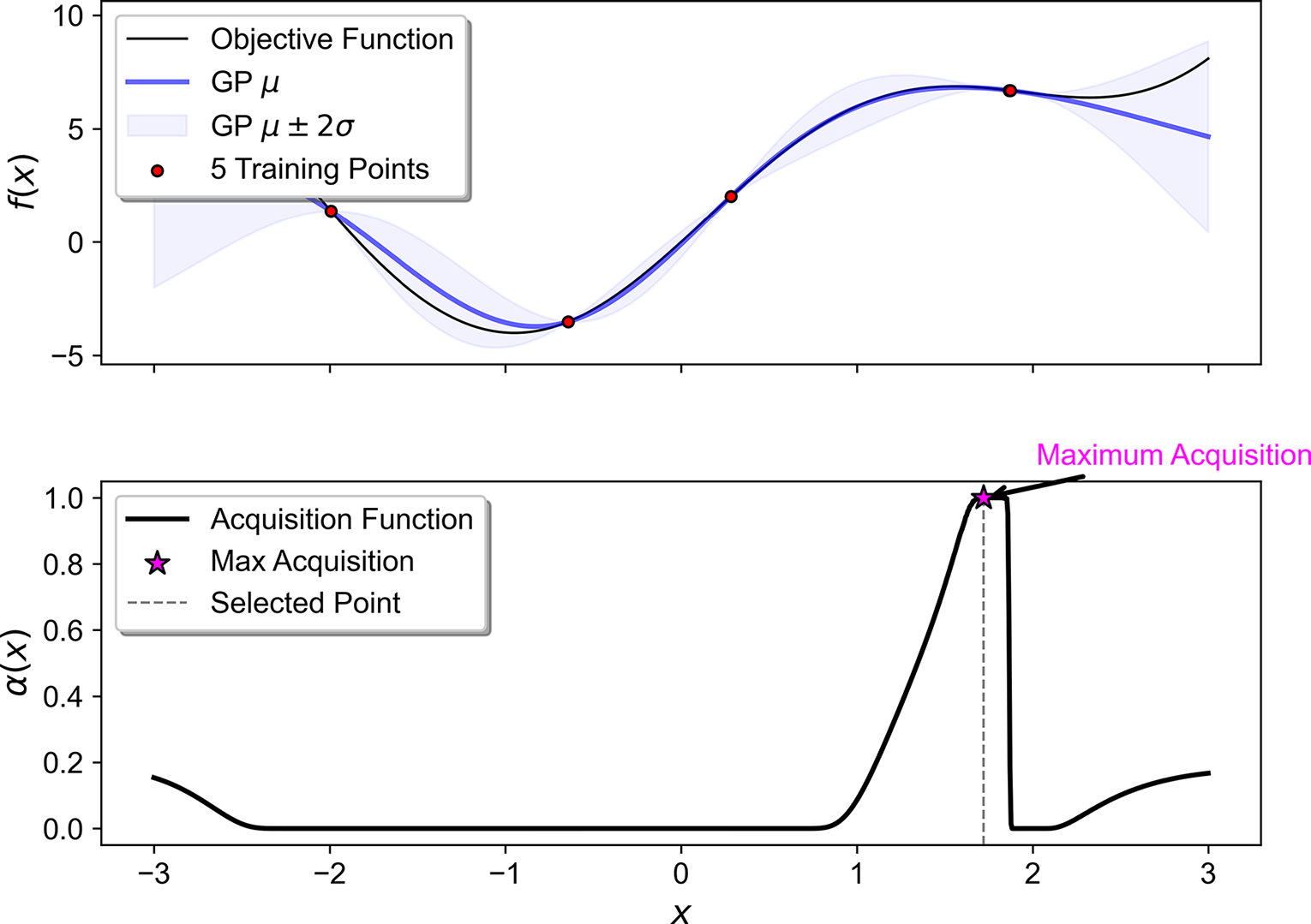


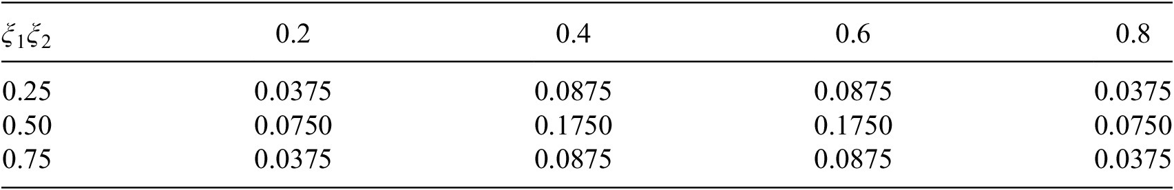

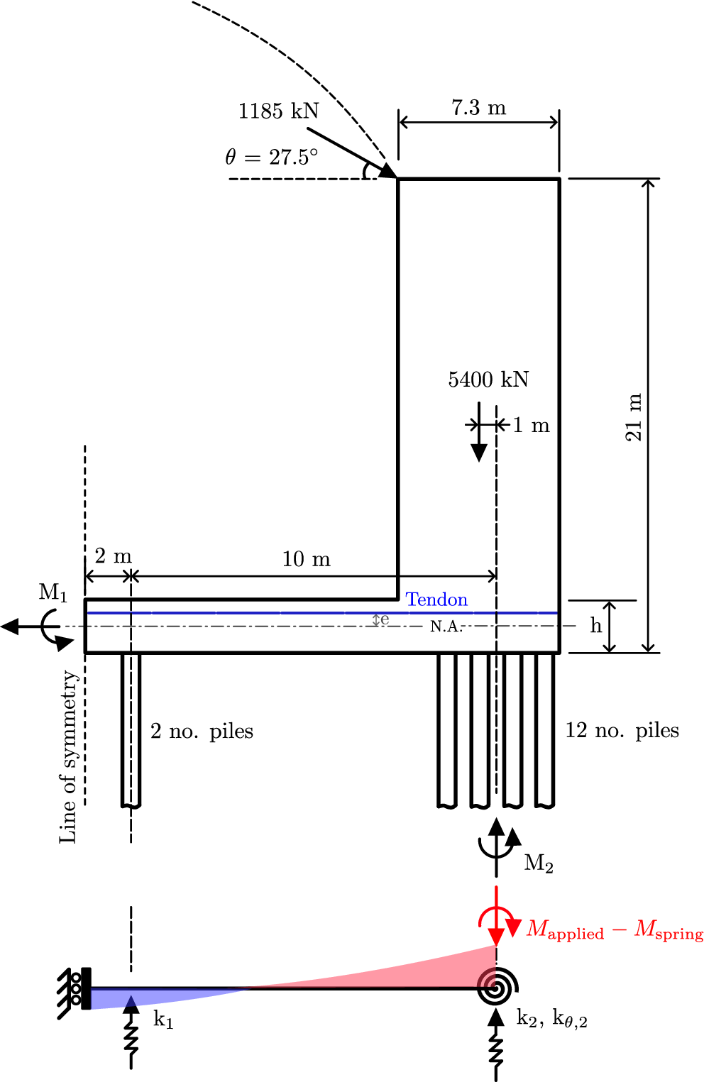


 Open access
Comments
No Comments have been published for this article.