


1. Introduction
Pension plans and other retirement products are characterized by long time horizons of 30–40 years. In many of them, the account value at retirement is transformed into a lifelong income using annuity factors. Sometimes, these factors are guaranteed when initiating the contract. The interest and longevity risk contained are, however, very difficult to analyze or quantify. During such long time horizons, substantial changes in the interest rate level or life expectancy can fundamentally change the value of annuity conversion factors.
This article proposes a computationally efficient algorithm for computing annuity conversion factorsFootnote
1
based on deep learning. Feed-forward neural networks (NNs) predict the factors based on the realization of the main risk factors at the time of retirement. A naive simulation of annuity factors suffers from the so-called “simulation-within-simulation” or nested simulation problem. Based on the realization of risk factors at the time of retirement (outer simulation), another simulation has to be carried out to compute the value of the annuity factor (inner simulation). This approach is often unfeasible or inefficient in practical applications. To circumvent the issue of nested simulations, several ideas were proposed to more efficiently carry out the outer simulation step. Feng et al. (Reference Feng, Li and Zhou2022) suggest reusing simulated random variables of the inner step (“green nested simulation”) and achieve a significant reduction of the simulation budget. Cairns (Reference Cairns2011) and Dowd et al. (Reference Dowd, Blake and Cairns2011) approximate the transformed (spot) survival probabilities by a second-order Taylor expansion. This immediately expresses the annuity factor as a function of the realization of the risk factors at the time of retirement. A similar approach using affine mortality models is Biffis & Millossovich (Reference Biffis and Millossovich2006). Closely related, least-squares Monte-Carlo (LSMC) algorithms were used to regress annuity factors on the realization of the underlying risk factors, see, for example, Bauer et al. (Reference Bauer, Bergmann and Reuss2010), Floryszczak et al. (Reference Floryszczak, Courtois and Majri2016), Ha & Bauer (Reference Ha and Bauer2022), Bacinello et al. (Reference Bacinello, Millossovich and Viviano2024). The link between Taylor expansions and LSMC to mortality-linked products is given by Bacinello et al. (Reference Bacinello, Millossovich and Viviano2021), one of the main references of this article. Hainaut & Akbaraly (Reference Hainaut and Akbaraly2023) combine LSMC with a $k$
-means clustering of the output variables (=local least squares). Similar to LSMC, many authors replace the inner simulation with feed-forward NNs. This seems to be especially promising if computations are based on many risk factors (see the examples of 12–20 risk factors by Castellani et al., Reference Castellani, Fiore, Marino, Passalacqua, Perla, Scognamiglio and Zanetti2021; Jonen et al., Reference Jonen, Meyhöfer and Nikolic2023; Krah et al., Reference Krah, Nikolic and Korn2020). An example of a smaller network size is Fernandez-Arjona, 2021.
$k$
-means clustering of the output variables (=local least squares). Similar to LSMC, many authors replace the inner simulation with feed-forward NNs. This seems to be especially promising if computations are based on many risk factors (see the examples of 12–20 risk factors by Castellani et al., Reference Castellani, Fiore, Marino, Passalacqua, Perla, Scognamiglio and Zanetti2021; Jonen et al., Reference Jonen, Meyhöfer and Nikolic2023; Krah et al., Reference Krah, Nikolic and Korn2020). An example of a smaller network size is Fernandez-Arjona, 2021.
In this article, we contribute to the comparison between LSMC and NN techniques. In previous research, it turned out that we need complex problems (12–20 risk factors) and complex NN structures (three layers) to slightly beat a simple LSMC with polynomial basis functions (see, for example, Castellani et al., Reference Castellani, Fiore, Marino, Passalacqua, Perla, Scognamiglio and Zanetti2021). Despite its simplicity, an LSMC with only 2–3 degree polynomials performs very well in many applications. Some authors see disadvantages of LSMC and find that LSMC algorithms do “not always produce satisfactory results” (Feng et al., Reference Feng, Li and Zhou2022), or “polynomials of higher degrees tend to explode beyond the fitting range” (Krah et al., Reference Krah, Nikolic and Korn2020). The aim of this article is to combine the advantages of LSMC and NN and work around reservations against them. In the case of deep learning and NNs, such reservations exist regarding the model interpretability (“black-box” techniques). For this reason, we follow a slightly different path compared to, for example, Castellani et al. (Reference Castellani, Fiore, Marino, Passalacqua, Perla, Scognamiglio and Zanetti2021). We represent LSMC as a small-sized NN architecture with a squared activation function. In other words, we represent LSMC as a special case of NN. This allows us to start with a NN architecture with a similar performance to LSMC. From this link between LSMC and NN, we have two advantages: (1) Small NNs are easy to handle and do not suffer from the curse of dimensionality or the choice of basis functions in LSMC. In NN, the complexity of model calibration depends on the number of layers and units per layer rather than the number of risk factors. (2) We can use the network structure to slightly extend LSMC, adding more neurons or layers to the network structure. With this approach, we can easily trade off between the interpretability of LSMC and the fitting capability of NN.
In our numerical analysis, we restrict ourselves to a specific model framework, a Li-Lee model for stochastic mortality and a two-factor Vasicek model for stochastic interest rates, see Günther & Hieber (Reference Günther and Hieber2024) for more background and further references on this model. It is straightforward to extend these results to more complex model frameworks. We compare our NN algorithm to the benchmark LSMC approach (see, for example, Bacinello et al., Reference Bacinello, Millossovich and Viviano2021). We consider different loss functions and show that it is promising to replace the least-squared error with the more general Huber loss function. We show that NNs achieve similar performance as LSMC techniques while not suffering from the curse of dimensionality. More complex models with many risk factors could therefore be handled more efficiently by NNs. These can be seen as an alternative to LSMC techniques, providing a more or less automatic and simultaneous selection of interaction terms and model calibration.
The article is organized as follows: Section 2 introduces the theoretical model framework and the NN architecture to approximate the value of annuity factors. Section 2 also shows how the NNs relate to LSMC algorithms as introduced in Bacinello et al., Reference Bacinello, Millossovich and Viviano2021. Section 3 shows how the NNs are calibrated. Section 4 presents an in-depth numerical analysis, discussing the choice of hyper-parameters for the deep learning approach and comparing the results to benchmark techniques.
2. Model framework and neural network architecture
We denote time by $t\gt 0$
and consider a cohort of individuals aged
$t\gt 0$
and consider a cohort of individuals aged $x$
at time
$x$
at time $t=0$
, retiring in
$t=0$
, retiring in $T \in \mathbb {N}$
years from now. To keep things simple, we consider two processes (interest rate risk by the short rate
$T \in \mathbb {N}$
years from now. To keep things simple, we consider two processes (interest rate risk by the short rate $\{r_{t}\}_{t\geq 0}$
and mortality risk by the central death rate
$\{r_{t}\}_{t\geq 0}$
and mortality risk by the central death rate $\{m_{x+t,t}\}_{t\geq 0}$
) on the probability space
$\{m_{x+t,t}\}_{t\geq 0}$
) on the probability space $(\Omega, \mathcal {G}, \mathbb {P})$
enlarged with a filtration
$(\Omega, \mathcal {G}, \mathbb {P})$
enlarged with a filtration $\{\mathcal {G}_t\}_{t \geq 0}$
accounting for mortality and financial risks, i.e.
$\{\mathcal {G}_t\}_{t \geq 0}$
accounting for mortality and financial risks, i.e. $\mathcal {G}_{t} = \mathcal {F}_{t} \vee \mathcal {H}_{t}$
. The sequence
$\mathcal {G}_{t} = \mathcal {F}_{t} \vee \mathcal {H}_{t}$
. The sequence $\{\mathcal {F}_{t}\}_{t\geq 0}$
filters the financial information
$\{\mathcal {F}_{t}\}_{t\geq 0}$
filters the financial information $\{r_{t}\}_{t\geq 0}$
and the sequence
$\{r_{t}\}_{t\geq 0}$
and the sequence $\{\mathcal {H}_{t}\}_{t \geq 0}$
describes the actuarial uncertainty
$\{\mathcal {H}_{t}\}_{t \geq 0}$
describes the actuarial uncertainty $\{m_{x+t,t}\}_{t\geq 0}$
.
$\{m_{x+t,t}\}_{t\geq 0}$
.
Since we are using a cohort approach, we consider future improvements in the central death rate after the retirement time $T$
and are interested in the realizations of
$T$
and are interested in the realizations of $m_{x+t, T+t}$
,
$m_{x+t, T+t}$
, $t = 0, 1, \ldots$
. This is opposed to a period approach where we would only consider the realized rates at the time of retirement
$t = 0, 1, \ldots$
. This is opposed to a period approach where we would only consider the realized rates at the time of retirement $T$
, i.e.
$T$
, i.e. $m_{x+T, T}$
for different ages
$m_{x+T, T}$
for different ages $x\in \mathbb {N}$
. For an extensive comparison of biometric indices under period- and cohort-based approaches, see Bacinello et al. (Reference Bacinello, Millossovich and Viviano2024). In our cohort-based approach, the future annuity factor at the retirement time
$x\in \mathbb {N}$
. For an extensive comparison of biometric indices under period- and cohort-based approaches, see Bacinello et al. (Reference Bacinello, Millossovich and Viviano2024). In our cohort-based approach, the future annuity factor at the retirement time $T$
is a conditional expectation given the information available up to the evaluation time
$T$
is a conditional expectation given the information available up to the evaluation time $T$
. If the
$T$
. If the $p$
risk factors
$p$
risk factors $\boldsymbol {Z_t} = (Z_1(t), Z_2(t) \ldots, Z_p(t)), t\geq 0$
, are Markov processes, the problem then translates into
$\boldsymbol {Z_t} = (Z_1(t), Z_2(t) \ldots, Z_p(t)), t\geq 0$
, are Markov processes, the problem then translates into
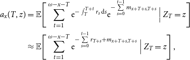 \begin{align} \nonumber a_x(T,\boldsymbol {z}) & = \mathbb {E}\Bigg [ \sum _{t=1}^{\omega -x - T}\mathrm {e}^{-\int _T^{T+t}r_s\,\textrm {d}s } \mathrm {e}^{-\sum \limits _{s=0}^{t-1} m_{x+T+s,T+s}} \,\Big |\, {\boldsymbol {Z_T}} = \boldsymbol {z}\Bigg ] \\ & \approx \mathbb {E}\Bigg [ \sum _{t=1}^{\omega -x - T} \mathrm {e}^{-\sum \limits _{s=0}^{t-1} r_{T+s} + m_{x+T+s,T+s}} \,\Big |\, {\boldsymbol {Z_T}} = \boldsymbol {z}\Bigg ] \,,\end{align}
where we assumed a maximal age $\omega$
of the individuals and
$\omega$
of the individuals and $z = (z_1, z_2, \ldots, z_p) \in \mathbb {R}^p$
. Closed-form solutions to Equation (1) are rare to obtain in practice unless the stochastic processes
$z = (z_1, z_2, \ldots, z_p) \in \mathbb {R}^p$
. Closed-form solutions to Equation (1) are rare to obtain in practice unless the stochastic processes $\{m_{x, t}\}_{t \geq 0}$
and
$\{m_{x, t}\}_{t \geq 0}$
and $\{r_{t}\}_{t \geq 0}$
are independent and of the affine form (Biffis, Reference Biffis2005; Luciano & Vigna Reference Luciano and Vigna2008).
$\{r_{t}\}_{t \geq 0}$
are independent and of the affine form (Biffis, Reference Biffis2005; Luciano & Vigna Reference Luciano and Vigna2008).
Note that the realization $\boldsymbol {z}$
of
$\boldsymbol {z}$
of $\boldsymbol {Z_T}$
is not known at
$\boldsymbol {Z_T}$
is not known at $t=0$
and is thus a stochastic variable itself. A naive approach to determine risk measures of the future annuity factors
$t=0$
and is thus a stochastic variable itself. A naive approach to determine risk measures of the future annuity factors $a_x(T, \boldsymbol {z})$
would require expensive nested Monte-Carlo simulations. In the following, we therefore want to provide efficient algorithms to compute
$a_x(T, \boldsymbol {z})$
would require expensive nested Monte-Carlo simulations. In the following, we therefore want to provide efficient algorithms to compute $a_x(T,\,\boldsymbol {z})$
as a function of the
$a_x(T,\,\boldsymbol {z})$
as a function of the $p$
risk factors
$p$
risk factors $Z_1, \ldots, Z_p$
that determine the interest rate
$Z_1, \ldots, Z_p$
that determine the interest rate $r_t$
and the mortality rate
$r_t$
and the mortality rate $m_{x,t}$
. Benchmark algorithms are LSMC techniques where the conditional expectation in (1) is obtained by comonotonic approximations or Taylor series expansions (Bacinello et al., Reference Bacinello, Millossovich and Viviano2021; Denuit, Reference Denuit2008; Dowd et al., Reference Dowd, Blake and Cairns2011; Hoedemakers et al., Reference Hoedemakers, Darkiewicz and Goovaerts2005; Liu, Reference Liu2013) rather than nested simulations.
$m_{x,t}$
. Benchmark algorithms are LSMC techniques where the conditional expectation in (1) is obtained by comonotonic approximations or Taylor series expansions (Bacinello et al., Reference Bacinello, Millossovich and Viviano2021; Denuit, Reference Denuit2008; Dowd et al., Reference Dowd, Blake and Cairns2011; Hoedemakers et al., Reference Hoedemakers, Darkiewicz and Goovaerts2005; Liu, Reference Liu2013) rather than nested simulations.
2.1 Approximation error
We want to find an approximating function of $a_x(T,\,\boldsymbol {z})$
using deep learning. Let us first introduce the approximating model
$a_x(T,\,\boldsymbol {z})$
using deep learning. Let us first introduce the approximating model ${e(\boldsymbol {z})} = e(z_1, \ldots, z_p)$
and define the distance to the true value
${e(\boldsymbol {z})} = e(z_1, \ldots, z_p)$
and define the distance to the true value $Y= a_{x}(T,\boldsymbol {z})$
by an error function
$Y= a_{x}(T,\boldsymbol {z})$
by an error function $L_\delta$
. In this article, we use the so-called Huber-loss function, which is a generalization of least-squared error. It is defined as:
$L_\delta$
. In this article, we use the so-called Huber-loss function, which is a generalization of least-squared error. It is defined as:
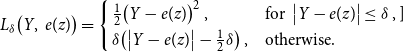 \begin{align*} L_{\delta }\big ( Y,\,e(\boldsymbol {z})\big ) = \left \{ \begin{array}{l@{\quad}l} \frac {1}{2}\big (Y-e(\boldsymbol {z}) \big )^2 \,, & \text {for }\ \big |Y-e(\boldsymbol {z})\big | \leq \delta \,,]\\[3pt] \delta \big (\big |Y-e(\boldsymbol {z})\big |-\frac {1}{2}\delta \big )\,, & \text {otherwise.} \end{array} \right . \end{align*}
The limit $\delta \rightarrow \infty$
corresponds to the special case of the least-squared error function
$\delta \rightarrow \infty$
corresponds to the special case of the least-squared error function $L_{\infty }\big ( Y,\,e(\boldsymbol {z})\big ) = \frac {1}{2}\big (Y-e(\boldsymbol {z}) \big )^2$
. For
$L_{\infty }\big ( Y,\,e(\boldsymbol {z})\big ) = \frac {1}{2}\big (Y-e(\boldsymbol {z}) \big )^2$
. For $\delta \lt \infty$
, the Huber loss reduces the squared effect of large deviations
$\delta \lt \infty$
, the Huber loss reduces the squared effect of large deviations $\big |Y-e(\boldsymbol {z})\big |$
and gives more flexibility in the error evaluation. We then determine the model that minimizes the loss, that is:
$\big |Y-e(\boldsymbol {z})\big |$
and gives more flexibility in the error evaluation. We then determine the model that minimizes the loss, that is:
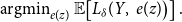 \begin{equation} \operatorname {argmin}\limits _{e(\boldsymbol {z})} \mathbb {E}\big [ L_\delta (Y,\,e(\boldsymbol {z}) \big ) \big ]\,. \end{equation}
To apply our algorithms, we simulate $n\in \mathbb {N}$
trajectories of the risk factors
$n\in \mathbb {N}$
trajectories of the risk factors $\Omega = \{\omega _{1}, \ldots, \omega _{n}\}$
leading to
$\Omega = \{\omega _{1}, \ldots, \omega _{n}\}$
leading to $n$
scenarios of the tuple
$n$
scenarios of the tuple $\big (Y^{(c)}, \boldsymbol {z}^{(c)}\big )$
,
$\big (Y^{(c)}, \boldsymbol {z}^{(c)}\big )$
, $c=1, \ldots, n$
. This can be used to determine a training sample estimate of (2) as:
$c=1, \ldots, n$
. This can be used to determine a training sample estimate of (2) as:
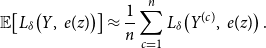 \begin{align} & \mathbb {E}\big [ L_\delta \big (Y,\,e(\boldsymbol {z}) \big ) \big ] \approx \frac {1}{n}\sum _{c=1}^n L_\delta \big (Y^{(c)},\,e(\boldsymbol {z}) \big )\,. \end{align}
2.2 Neural network architecture
We consider a NN architecture with $J \in \mathbb {N}$
layers and
$J \in \mathbb {N}$
layers and $N^{(j)} \in \mathbb {N}$
neurons per layer, for
$N^{(j)} \in \mathbb {N}$
neurons per layer, for $j=1, 2, \ldots, J.$
Every neuron
$j=1, 2, \ldots, J.$
Every neuron $k=1,2,\ldots, N^{\left ({j}\right )}$
in a layer
$k=1,2,\ldots, N^{\left ({j}\right )}$
in a layer $j$
is activated by an activation function of the type
$j$
is activated by an activation function of the type $\phi _k^{(j)}(x)$
. The first layer is defined as:
$\phi _k^{(j)}(x)$
. The first layer is defined as:
 \begin{align} y_{k}^{(1)} = \phi _{k}^{(1)}\Big (\beta _{0,k}^{(1)}+\beta _{1,k}^{(1)}z_1 + \ldots \beta _{p,k}^{(1)}z_p\Big )\,, \end{align}
where we define weights $\beta _{1,k}^{(1)} \in \mathbb {R}$
and intercepts
$\beta _{1,k}^{(1)} \in \mathbb {R}$
and intercepts $\beta _{0,k}^{(1)} \in \mathbb {R}$
for
$\beta _{0,k}^{(1)} \in \mathbb {R}$
for $k=1,2,\ldots, N^{\left ({1}\right )}$
. The activation function
$k=1,2,\ldots, N^{\left ({1}\right )}$
. The activation function $\phi _{k}^{(1)}$
needs to be chosen appropriately. The outputs
$\phi _{k}^{(1)}$
needs to be chosen appropriately. The outputs $y_{k}^{(1)}$
are used as inputs for the second layer. In the
$y_{k}^{(1)}$
are used as inputs for the second layer. In the $j-th$
layer, for
$j-th$
layer, for $j=2, \ldots, J-1$
, we have
$j=2, \ldots, J-1$
, we have
 \begin{align} y_{k}^{(j)} = \phi _{k}^{(j)}\bigg (\beta _{0,k}^{(j)}+\sum \limits _{l=1}^{N^{(j-1)}}\beta _{l,k}^{(j)}\cdot y_{l}^{(j-1)}\bigg )\,, \end{align}
where, in each layer $j$
, we have weights and intercepts
$j$
, we have weights and intercepts $\beta _{l,k}^{(j)}$
,
$\beta _{l,k}^{(j)}$
, $l = 1, 2, \ldots, N^{(j-1)}$
,
$l = 1, 2, \ldots, N^{(j-1)}$
, $k=1,2,\ldots, N^{\left ({j}\right )}$
. The last layer then provides the final output of the NN:
$k=1,2,\ldots, N^{\left ({j}\right )}$
. The last layer then provides the final output of the NN:
 \begin{align} e(\boldsymbol {z}) = y_{1}^{(J)} = \phi _{1}^{(J)} \bigg (\beta _{0,1}^{(J)}+ \sum \limits _{l=1}^{N^{(J)}} \beta _{l,1}^{(J)} \cdot y_{l}^{(J-1)} \bigg )\,. \end{align}
2.3 Least squares Monte-Carlo as special case
LSMC techniques were originally introduced in Finance by Longstaff and Schwartz, 2001 to price American options. The technique involves numerical approximations of functional payoffs through affine combinations of basis functions. Common choices in the literature include Hermite, Laguerre or Chebychev polynomials; however, in many applications, expansions of up to 2nd order polynomials are already able to catch much of the variation in the data (see Cairns, Reference Cairns2011; Longstaff & Schwartz, Reference Longstaff and Schwartz2001). In our example, an approximation by $M$
basis functions
$M$
basis functions $e_{l}\big (\boldsymbol {z}\big )$
,
$e_{l}\big (\boldsymbol {z}\big )$
, $l=0,1,\ldots, M-1$
would lead to the model:
$l=0,1,\ldots, M-1$
would lead to the model:
 \begin{align} e(\boldsymbol {z}) = \sum _{l=0}^{M-1}\beta _{l}\cdot e_{l}\big (\boldsymbol {z}\big )\,. \end{align}
LSMC was employed in lattice structures to approximate the continuation value of the American option under a discrete-time framework. Therefore, the basis representation (7) was obtained by regressing over the state variable(s) and basis functions. LSMC is used to compute capital requirements and balance sheet projections in life insurance where computations are otherwise based on a nested simulation approach, see Bauer et al. (Reference Bauer, Bergmann and Reuss2010).
A two-dimensional NN ( $J=2$
) can be parameterized to resemble the basis functions of a LSMC algorithm. To illustrate this, Example 2.1 gives the polynomial basis functions used by Bacinello et al. (Reference Bacinello, Millossovich and Viviano2021) and embeds this as a NN appropriately choosing activation functions. Note that this example can be generalized to more risk factors and higher degrees of the basis functions.
$J=2$
) can be parameterized to resemble the basis functions of a LSMC algorithm. To illustrate this, Example 2.1 gives the polynomial basis functions used by Bacinello et al. (Reference Bacinello, Millossovich and Viviano2021) and embeds this as a NN appropriately choosing activation functions. Note that this example can be generalized to more risk factors and higher degrees of the basis functions.
Example 2.1 (LSMC, 3rd order expansion). Let our model comprise two risk factors $\boldsymbol {Z} = (Z_1, Z_2)$
, where
$\boldsymbol {Z} = (Z_1, Z_2)$
, where $Z_1$
describes the state of the interest rate process
$Z_1$
describes the state of the interest rate process $r_T$
and
$r_T$
and $Z_2$
describes the state of the central death rate
$Z_2$
describes the state of the central death rate $m_{x+T,T}$
. Consider the expansion (7) and the
$m_{x+T,T}$
. Consider the expansion (7) and the $M=7$
basis functions
$M=7$
basis functions
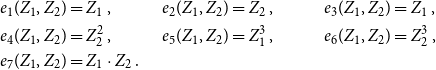 \begin{alignat*} {4} e_{1}(Z_{1},Z_{2})&=\,&&Z_{1}\,, \qquad \quad &&e_{2}(Z_{1},Z_{2})=Z_{2}\,, \qquad \quad &&e_{3}(Z_{1},Z_{2})=Z_{1}\,,\\ e_{4}(Z_{1},Z_{2})&=&&Z_{2}^2\,,&&e_{5}(Z_{1},Z_{2})=Z_{1}^3\,, &&e_{6}(Z_{1},Z_{2})=Z_{2}^3\,, \\ e_{7}(Z_{1},Z_{2})&=&&Z_{1}\cdot Z_2\,. \end{alignat*}
We can choose weights and activation functions in the first layer of the NN to represent this with $N^{(1)}=6$
neurons. In (4), this means that we choose
$N^{(1)}=6$
neurons. In (4), this means that we choose $\phi _{1}^{(1)}(z) = \phi _{2}^{(1)}(z) = z$
,
$\phi _{1}^{(1)}(z) = \phi _{2}^{(1)}(z) = z$
, $\phi _{k}^{(1)}(z) = z^2$
for
$\phi _{k}^{(1)}(z) = z^2$
for $k=3,4,7,8$
and
$k=3,4,7,8$
and $\phi _{k}^{(1)}(z) = z^3$
for
$\phi _{k}^{(1)}(z) = z^3$
for $k=5,6$
. The weights
$k=5,6$
. The weights $\beta _{i,k}^{(1)}$
,
$\beta _{i,k}^{(1)}$
, $i=0,1,2$
, are then chosen appropriately such that:
$i=0,1,2$
, are then chosen appropriately such that:
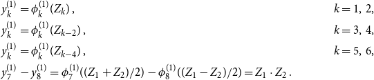 \begin{align*} & y_{k}^{(1)} = \phi _{k}^{(1)}(Z_k)\,, & k=1,\,2, \\ & y_{k}^{(1)} = \phi _{k}^{(1)}(Z_{k-2})\,, & k=3,\,4, \\ & y_{k}^{(1)} = \phi _{k}^{(1)}(Z_{k-4})\,, & k=5,\,6, \\ & y_{7}^{(1)} - y_{8}^{(1)} = \phi _{7}^{(1)}((Z_1+Z_2)/2) - \phi _{8}^{(1)}((Z_1-Z_2)/2) = Z_1 \cdot Z_2 \,. & \end{align*}
With this, the output (6) of the NN with one hidden layer can be chosen to be identical to the least-squares basis function expansion (7).
3. Calibrating the neural network
The calibration of the NN architecture is carried out based on the tuple $\big (Y^{(c)}, \boldsymbol {z}^{(c)}\big )$
, for
$\big (Y^{(c)}, \boldsymbol {z}^{(c)}\big )$
, for $c=1, \ldots, n$
, as introduced in Section 2.1. In our case, these were obtained by simulation from some economic scenario generator.
$c=1, \ldots, n$
, as introduced in Section 2.1. In our case, these were obtained by simulation from some economic scenario generator.
Algorithm 3.1 (Calibrating the NN). The calibration then works in the following steps:
-
1. Determine the outer scenarios $\boldsymbol {z}^{(c)} = z_1^{(c)}, \ldots, z_p^{(c)}$
for
$c = 1, \ldots, n$
.
$\boldsymbol {z}^{(c)} = z_1^{(c)}, \ldots, z_p^{(c)}$
for
$c = 1, \ldots, n$
. -
2. For each outer scenario
$c=1, \ldots, n$
, compute inner scenarios to obtain an estimate for
$Y^{(c)}$
as described in Section
2.1
. -
3. Specify the NN architecture, that is the number of layers
$J$
, the number of neurons
$N^{(j)}$
in each layer, and the activation functions.
-
4. Use the back-propagation algorithm and the objective function (2) to calculate all weights
$\beta _{l,k}^{(j)}$
of the NN.


As activation functions, we will use the Square activation function:
 \begin{equation*} \operatorname {Square}(z)=z^{2}\,, \end{equation*}
and the Exponential Linear Units ( $a \in \mathbb {R}^{+}$
) activation function:
$a \in \mathbb {R}^{+}$
) activation function:
 \begin{equation*} \text {Elu}(z)= \begin{cases} z\,,\ & \text {if }z \geq 0\,, \\ a\left (\mathrm {e}^{z}-1\right ),\,\ & \text {if }z\lt 0. \end{cases} \end{equation*}
For more details on possible activation functions and hyperparameter selection, please refer to the appendices of the paper.
4. Numerical results and comparison
In this section, we analyze the performance of the NN architecture to approximate annuity factors, discuss the choice of hyper-parameters, and compare to LSMC.
4.1 Exemplary financial and actuarial model
We use an exemplary financial and actuarial model that is used for solvency assessment and regulation in central Europe, see Günther & Hieber (Reference Günther and Hieber2024) for a discussion and background of this model. Mortality is modeled by a Li-Lee multi-population model (Li & Lee, Reference Li and Lee2005):
 \begin{equation} \ln (m_{x,t}) = \ln (m_{x,t}^{\textrm {g}}) + \ln (m_{x,t}^{\textrm {c}})\,, \end{equation}
where $m_{x,t}^{\textrm {g}}$
describes the mortality of a larger general population and
$m_{x,t}^{\textrm {g}}$
describes the mortality of a larger general population and $m_{x,t}^{\textrm {c}}$
defines the country-specific deviation from the general trend. In particular, we have
$m_{x,t}^{\textrm {c}}$
defines the country-specific deviation from the general trend. In particular, we have
 \begin{align*} \ln (m_{x,t}^{\textrm {g}}) &= A_{x}+B_{x}K_{t}\,,\\ \ln (m_{x,t}^{\textrm {c}}) &= a_{x}+b_{x}k_{t}\,, \end{align*}
where $a_{x}, A_x\in \mathbb {R}$
describe the age-specific pattern of mortality,
$a_{x}, A_x\in \mathbb {R}$
describe the age-specific pattern of mortality, $k_{t}, K_t\in \mathbb {R}$
represent the time trend of death rates, and
$k_{t}, K_t\in \mathbb {R}$
represent the time trend of death rates, and $b_{x}, B_x \in \mathbb {R}$
measure the loading to the particular age groups when the mortality indices
$b_{x}, B_x \in \mathbb {R}$
measure the loading to the particular age groups when the mortality indices $k_{t}, K_t$
change. The mortality improvement factor
$k_{t}, K_t$
change. The mortality improvement factor $K_{t}$
evolves as a Brownian motion with drift, while
$K_{t}$
evolves as a Brownian motion with drift, while $k_t$
is assumed to behave as an auto-regressive process of order 1. Thus, we assume
$k_t$
is assumed to behave as an auto-regressive process of order 1. Thus, we assume
 \begin{align*} K_t &= K_{t-1} + \gamma + \epsilon _t\,, \\ k_t &= c + d \cdot k_{t-1} + \delta _t\,, \end{align*}
where $\epsilon _t \sim \mathcal {N}(0, \sigma _\epsilon ^2)$
and
$\epsilon _t \sim \mathcal {N}(0, \sigma _\epsilon ^2)$
and $\delta _t \sim \mathcal {N}(0, \sigma _\delta ^2)$
are i.i.d. error terms, while
$\delta _t \sim \mathcal {N}(0, \sigma _\delta ^2)$
are i.i.d. error terms, while $\gamma$
,
$\gamma$
, $c$
,
$c$
, $d \in \mathbb {R}$
define the two auto-regressive processes.
$d \in \mathbb {R}$
define the two auto-regressive processes.
The model is calibrated on data from North-Western European countries with a specific focus on the deviation of the Swiss subpopulation. The data are available on the Human Mortality Database via https://www.mortality.org . On the financial side, we assume a two-factor Vasicek model for the interest rate:
 \begin{align} & r_t = \psi _t + x_t + y_t \,, \nonumber\\ & \mathrm {d} x_t = -\alpha \, x_t \, \mathrm {d} t + \nu \,\mathrm {d} W_t^{(1)}\,, \nonumber \\ & \mathrm {d} y_t = -\beta \, y_t \, \mathrm {d} t + \eta \Big ( \rho \, \mathrm {d} W_t^{(1)} + \sqrt {1 - \rho ^2}\, \mathrm {d} W_t^{(2)} \Big ) \,, \nonumber \\ & \psi _t = f^M(0,t) + \frac {\nu ^2}{2} \cdot g_a(t)^2 + \frac {\eta ^2}{2} \cdot g_b(t)^2 + \rho \nu \eta \cdot g_a(t) \cdot g_b(t)\,, \end{align}
where $x$
and
$x$
and $y$
describe short- and long-term deviations from the deterministic function
$y$
describe short- and long-term deviations from the deterministic function $\psi _t$
, which contains the initial forward-yield curve
$\psi _t$
, which contains the initial forward-yield curve $f^M(0,t)$
. The parameters
$f^M(0,t)$
. The parameters $\alpha \gt 0, \beta \gt 0$
describe the mean reversion speed of the two processes
$\alpha \gt 0, \beta \gt 0$
describe the mean reversion speed of the two processes $x$
and
$x$
and $y$
, while
$y$
, while $\nu \gt 0, \eta \gt 0$
define their volatilities. The Brownian motions
$\nu \gt 0, \eta \gt 0$
define their volatilities. The Brownian motions $W_t^{(1)}$
and
$W_t^{(1)}$
and $W_t^{(2)}$
are independent and the correlation between the two processes
$W_t^{(2)}$
are independent and the correlation between the two processes $x$
and
$x$
and $y$
is given by
$y$
is given by $\rho$
. The initial forward yield curve follows a Nelson-Siegel-Svensson yield curve:
$\rho$
. The initial forward yield curve follows a Nelson-Siegel-Svensson yield curve:
 \begin{align*} & f^M(0,t) = \beta _0 + \beta _1 \frac {\theta _1}{t}\Big (1 - \mathrm {e}^{- \frac {t}{\theta _1}}\Big ) + \beta _2 \frac {\theta _1}{t}\left (1 - \mathrm {e}^{- \frac {t}{\theta _1}}\frac {t+\theta _1}{\theta _1}\right ) + \beta _3 \frac {\theta _2}{t}\left (1 - \mathrm {e}^{- \frac {t}{\theta _1}} \frac {t+\theta _2}{\theta _2}\right )\,. \end{align*}
and its parameters are taken from estimations by the German Federal Bank from November 2023. The remaining parameters are adapted from Graf et al. (Reference Graf, Kling and Ruß2021) and Günther & Hieber (Reference Günther and Hieber2024), see also the Appendix C.
To summarize, the Markov process $\boldsymbol {Z_t}$
describing the central death rate as well as the interest rate process is composed of the four risk factors
$\boldsymbol {Z_t}$
describing the central death rate as well as the interest rate process is composed of the four risk factors $K_t$
,
$K_t$
, $k_t$
,
$k_t$
, $x_t$
, and
$x_t$
, and $y_t$
, that is
$y_t$
, that is
 \begin{equation*}z_t = (Z_1(t), Z_2(t), Z_3(t), Z_4(t)) = (K_t, k_t, x_t, y_t)\,.\end{equation*}
Note that these risk factors are uniquely determined by the innovations $\epsilon _t, \delta _t, W_t^{(1)}$
and
$\epsilon _t, \delta _t, W_t^{(1)}$
and $W_t^{(2)}$
. In practice, we replace the risk factors with their corresponding normally-distributed innovations, as most training algorithms for NNs are optimized for standardized input data.
$W_t^{(2)}$
. In practice, we replace the risk factors with their corresponding normally-distributed innovations, as most training algorithms for NNs are optimized for standardized input data.
4.2 Numerical results
We compare the results from the NN method as described in Algorithm 3.1 with those from the LSMC approach. To estimate the error of both techniques, we compute a benchmark approximation based on a nested simulation with $100\,000$
outer and
$100\,000$
outer and $100\,000$
inner simulations.
$100\,000$
inner simulations.
We run the NN and the LSMC algorithm 100 times to get a reliable estimate and confidence intervals of the average error for both methods. For each run $i$
, we employ a new nested simulation with
$i$
, we employ a new nested simulation with $1\,000$
outer and 10 inner scenarios that serve as the input for both algorithms. After fitting the two models, we can rapidly compute the estimated results for a large number of scenarios. To this end, we generate a new set of
$1\,000$
outer and 10 inner scenarios that serve as the input for both algorithms. After fitting the two models, we can rapidly compute the estimated results for a large number of scenarios. To this end, we generate a new set of $1\,000\,000$
outer scenarios
$1\,000\,000$
outer scenarios ${\boldsymbol {z}}^{(c)}$
and compute their corresponding estimated annuity values
${\boldsymbol {z}}^{(c)}$
and compute their corresponding estimated annuity values $\hat {Y}^{(c)}$
,
$\hat {Y}^{(c)}$
, $c=1, \ldots, 1\,000\,000$
.
$c=1, \ldots, 1\,000\,000$
.
We measure the performance of both techniques on the $90^{\mathrm {th}}$
percentile
$90^{\mathrm {th}}$
percentile $q_{90\%}^{(i),\mathrm {LSMC/NN}}$
of the annuity values
$q_{90\%}^{(i),\mathrm {LSMC/NN}}$
of the annuity values $\hat {Y}^{(c)}$
at
$\hat {Y}^{(c)}$
at $t=1$
. Finally, we compute the Mean Absolute Percentage Error (MAPE) over all 100 runs:
$t=1$
. Finally, we compute the Mean Absolute Percentage Error (MAPE) over all 100 runs:
 \begin{equation*} \mathrm {MAPE}^{\mathrm {LSMC/NN}} = \frac {1}{100} \sum _{i=1}^{100} \Bigg | \frac {q_{90\%}^{(i), \mathrm {LSMC/NN}} - q_{90\%}^{\mathrm {true}}}{q_{90\%}^{\mathrm {true}}} \Bigg | \,. \end{equation*}
For the LSMC algorithm, we use polynomials up to degree $d = 2$
as a basis. This is in line with the work by Bacinello et al. (Reference Bacinello, Millossovich and Viviano2021), who show that polynomials of higher degrees do not result in an improvement in the accuracy for a problem of this complexity.
$d = 2$
as a basis. This is in line with the work by Bacinello et al. (Reference Bacinello, Millossovich and Viviano2021), who show that polynomials of higher degrees do not result in an improvement in the accuracy for a problem of this complexity.
We set up the NN with one hidden layer, in which we use either an exponential linear unit (ELU) or a square as an activation function. The single neuron in the output layer is not transformed by any activation function. Fine-tuning the remaining hyper-parameters of the NN and the backpropagation algorithm is a delicate task. After several initial experiments, we decided to use a decaying learning rate which is initialized at $0.003$
and run the backpropagation algorithm for
$0.003$
and run the backpropagation algorithm for $E = 100$
epochs at a batch size of
$E = 100$
epochs at a batch size of $B = 128$
. We use the packages keras and tensorflow for the implementation.
$B = 128$
. We use the packages keras and tensorflow for the implementation.
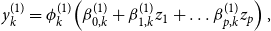
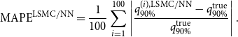
Fig. 1 compares the MAPE of the NN algorithm with that of the LSMC for different loss functions. After 100 epochs and for all loss functions, we can see that with an increasing number of neurons, the error decreases from between 0.4% and 2% for just one neuron in the hidden layer to below 0.2% for 20 neurons. For networks with fewer than five neurons in the hidden layer, the Elu activation function outperforms the Square activation function. On the other hand, for networks with a larger number of neurons, this advantage is less pronounced and even reversed for the Mean Squared Error and Huber loss functions. The most convincing results are obtained when combining the quadratic activation function in the hidden layer with a Huber loss function. Here, the confidence intervals of the NN approach and the LSMC method overlap after 8 neurons in the hidden layer.
Relative error of the MC simulations and the LSMC and neural network algorithms as a function of the number of neurons $N$
in the hidden layer for different activation functions and loss functions. Corresponding 95% confidence intervals in shaded colors.
$N$
in the hidden layer for different activation functions and loss functions. Corresponding 95% confidence intervals in shaded colors.
However, the NNs are still slightly outperformed by the LSMC approach. It achieves an average MAPE of 0.10%, while the NN approach with 20 neurons and a quadratic activation function remains at 0.11% MAPE. This can be explained by several factors. First, $1\,000$
input samples and 4 explanatory variables are very small numbers for NNs. Their strength might come into play for more complex problems with a multitude of variables and possible interaction effects. Secondly, using only 10 inner scenarios leaves us with very noisy estimations of the annuity factors in each outer scenario. Thus, the LSMC approach is at an advantage, because it imposes a well-defined structure on the estimation problem. In contrast to the NN approach, the training for the LSMC only requires a matrix inversion which is computationally fast for a small number of risk factors. Thus, the LSMC algorithm only took an average of 2.3 s of computation time, while the NN algorithm terminated after an average of 21.5 s. The number of neurons in the hidden layer does not considerably affect the computation time. The Monte Carlo simulations used for both algorithms took an average of 0.2 s while being around 10 times less accurate.
$1\,000$
input samples and 4 explanatory variables are very small numbers for NNs. Their strength might come into play for more complex problems with a multitude of variables and possible interaction effects. Secondly, using only 10 inner scenarios leaves us with very noisy estimations of the annuity factors in each outer scenario. Thus, the LSMC approach is at an advantage, because it imposes a well-defined structure on the estimation problem. In contrast to the NN approach, the training for the LSMC only requires a matrix inversion which is computationally fast for a small number of risk factors. Thus, the LSMC algorithm only took an average of 2.3 s of computation time, while the NN algorithm terminated after an average of 21.5 s. The number of neurons in the hidden layer does not considerably affect the computation time. The Monte Carlo simulations used for both algorithms took an average of 0.2 s while being around 10 times less accurate.
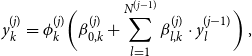
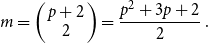
However, NNs come very close to the accuracy of the LSMC algorithm and are not subject to the curse of dimensionality. As illustrated in Fig. 2, the time spent on the NN algorithm does not rely significantly on the number of risk factors. The LSMC algorithm, on the other hand, takes around 10 times as long when increasing the number of risk factors from 1 to 4. The number of basis functions $m$
for polynomials of
$m$
for polynomials of $p$
risk factors up to degree 2 is
$p$
risk factors up to degree 2 is
 \begin{equation*} m = \left (\begin{array}{c} p+2 \\ 2 \end{array}\right ) = \frac {p^2+3p+2}{2}\,. \end{equation*}
Efficient algorithms for inverting matrices of dimension $m\times m$
as described in Pan & Reif (Reference Pan and Reif1985) are based on the Newton method, which relies on matrix multiplications. Thus, the complexity of a matrix inversion is at least
$m\times m$
as described in Pan & Reif (Reference Pan and Reif1985) are based on the Newton method, which relies on matrix multiplications. Thus, the complexity of a matrix inversion is at least $\mathcal {O}(m^2) = \mathcal {O}(p^4)$
. Adding more risk factors, we expect to see a break-even point beyond which it is numerically more expensive to use the LSMC algorithm. To this end, we can interpret a NN that uses the Mean Squared Error as its loss function and a Square activation function as an alternative way to simultaneously calibrate and select the interaction terms of an LSMC approach. Note that computing the annuity factors for
$\mathcal {O}(m^2) = \mathcal {O}(p^4)$
. Adding more risk factors, we expect to see a break-even point beyond which it is numerically more expensive to use the LSMC algorithm. To this end, we can interpret a NN that uses the Mean Squared Error as its loss function and a Square activation function as an alternative way to simultaneously calibrate and select the interaction terms of an LSMC approach. Note that computing the annuity factors for $n$
cohorts would require us to apply the NN algorithm or the LSMC algorithm
$n$
cohorts would require us to apply the NN algorithm or the LSMC algorithm $n$
times, respectively. However, we can reuse the simulated realizations of the random variables
$n$
times, respectively. However, we can reuse the simulated realizations of the random variables $\epsilon _t, \delta _t, W_t^{(1)}$
and
$\epsilon _t, \delta _t, W_t^{(1)}$
and $W_t^{(2)}$
for the Monte-Carlo simulation in both algorithms.
$W_t^{(2)}$
for the Monte-Carlo simulation in both algorithms.
The computation time in seconds spent on running the LSMC algorithm and the neural network algorithm for 100 epochs in relation to the number of risk factors $p$
.
$p$
.
5. Conclusion
In this article, we investigate deep learning techniques for annuity factor estimation. When the annuitisation of capital is due at a future time point, closed-form analytical solutions are generally not available. We compare feed-forward NNs to the LSMC technique. We obtain the following results: Surprisingly, NNs cannot outperform the accuracy of the LSMC algorithm. However, the combination of the squared activation function and Huber loss function can already help small network sizes replicate the LSMC technique. This connection between LSMC techniques and NNs (as presented in Example 2.1) is a promising approach to profit at the same time from the interpretability of the LSMC technique and the almost automatic calibration of the NN architecture. This calibration avoids the tedious choice of interaction terms for LSMC techniques and does not suffer from the curse of dimensionality if many risk factors are needed.
Data availability statement
Data availability does not apply to our research because we use a simulation-based dataset.
Funding statement
This work received no specific grant from any funding agency, commercial, or not-for-profit sectors.
Competing interests
None.
Appendix A. Choice of activation functions
Step 3 in the algorithm leaves a lot of freedom on how to specify the neural network architecture. The annuity factors (1) we want to predict are defined on the positive half-plane $[0,\infty )$
. We want to avoid activation functions whose range is bounded from above, such as sigmoid or tanh. Therefore, we consider:
$[0,\infty )$
. We want to avoid activation functions whose range is bounded from above, such as sigmoid or tanh. Therefore, we consider:
-
• Rectified Linear Units
\begin{equation*} \text {ReLU}(z) = \max \{0,\ z\}\,, \end{equation*}
-
• Gaussian Error Linear Units
\begin{equation*} \text {Gelu}(z) = z\frac {1}{2}\left [1+\operatorname {erf}\left (\frac {z}{\sqrt {2}}\right )\right ]\,, \end{equation*}
-
• Exponential Linear Units (
$a \in \mathbb {R^{+}}$
)
\begin{equation*} \text {Elu}(z)= \begin{cases} z\,,\ & \text {if }z \geq 0\,, \\ a\left (e^{z}-1\right ),\,\ & \text {if }z\lt 0\,, \end{cases} \end{equation*}
-
• Scaled Exponential Linear Units (
$\tau, \, a \in \mathbb {R^{+}}$
)
\begin{equation*} \text {Selu}(z) = \begin{cases} \tau \cdot z\,,\ & \text {if }z\gt 0 \\ \tau \cdot \alpha \left (e^{z}-1\right )\,,& \text {if }z\leq 0\,, \end{cases} \end{equation*}
-
• Softplus
\begin{equation*} \text {Softp}(z)=\ln (1+e^{z})\,, \end{equation*}
-
• Softsign
\begin{equation*} \text {Softs}(z) = \left (\frac {z}{|z|+1}\right )\,, \end{equation*}
-
• Swish
\begin{equation*} \text {Swish}(z) = \frac {z}{1+e^{-z}}\,, \end{equation*}
-
• Square
\begin{equation*} \operatorname {Square}(z)=z^{2}\,, \end{equation*}
-
• Cubic
\begin{equation*} \operatorname {Cubic}(z)=z^{3}\,. \end{equation*}


Appendix B. Choice of other hyper-parameters
Apart from the choice of activation function, the neural network architecture allows for more flexibility by a variety of hyper-parameters:
-
• The network depth, that is the number of layers
$J$
. Since Cybenko (Reference Cybenko1989), it is acknowledged that any continuous function can be approximated by a single-layer neural network. Explicit solutions for the construction of the network architecture in terms of depth and hyperparameter selection to achieve a target degree of precision are hard to obtain in practice and only approximation bounds are available (Yarotsky, Reference Yarotsky2017). -
• The layer dimension,
$N^{\left (j\right )}$
. The drawback of improvements based on the layers’ dimension is that computational time increases in the number of neurons since those represent additional units to be optimized during the learning phase. -
• Pre-processing and regularization. It is possible to envisage specific layers which are aimed at flattening the data input, to shuffle and/or induce sparsity by regularisation or dropout techniques, to improve the standardization efficiency by batch or layer-tailored solutions (Bengio, Reference Bengio2012; Goodfellow et al., Reference Goodfellow, Bengio and Courville2016).
-
• The optimization routine. Repeated local optimization over small batches is generally preferred to a globally implemented routine. Batch size
$B$
and epochs
$E$
, i.e. the sub-sample sizes over which to optimize and the number of iterations to be performed while implementing the routine are discretionary interventions on the learning routine proficiency. If the representative capability is expected to improve over the number of training epochs up to a convergence rate, for the batch size a trade-off between accuracy and over-fitting generally holds.


Appendix C. Choice of parameters for mortality and interest rates
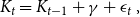
The parameters of the financial market are described in Table A.1.
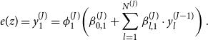
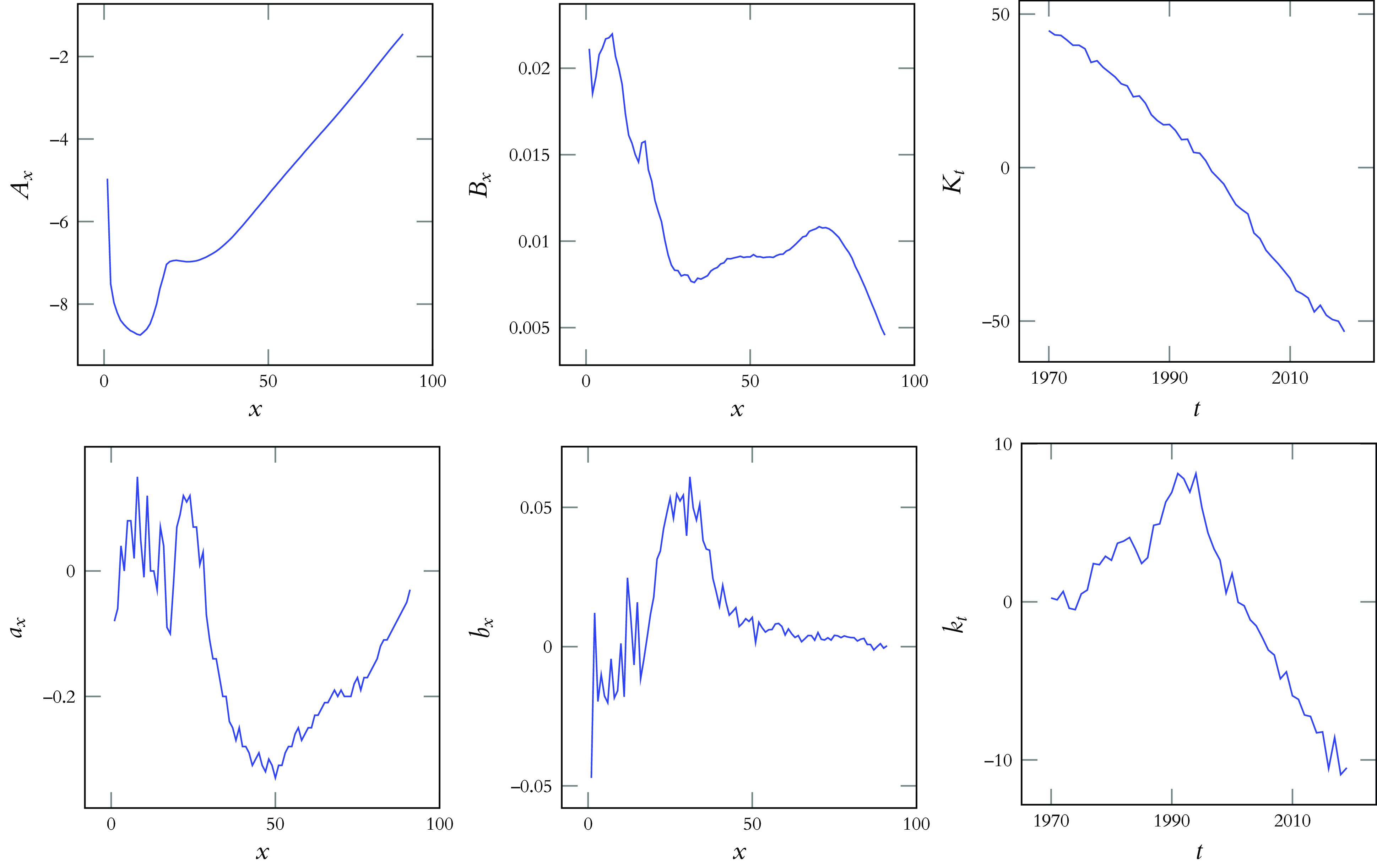
The general population in the Li-Lee model has been from the countries of Austria, Belgium, Denmark, Finland, France, Germany, Iceland, Ireland, Luxembourg, the Netherlands, Norway, Sweden, Switzerland and the United Kingdom. Fig. 3 presents the calibrated parameters. Future developments of the mortality improvements $K_t$
of the North-Western European population are modeled as
$K_t$
of the North-Western European population are modeled as
 \begin{align*} K_t = K_{t-1} + \gamma + \epsilon _t\,, \end{align*}
with drift $\gamma = -2.0014$
and
$\gamma = -2.0014$
and $\epsilon _t \sim \mathcal {N}(0, 2.4180)$
. The future development of the parameter
$\epsilon _t \sim \mathcal {N}(0, 2.4180)$
. The future development of the parameter $k_t$
for the Swiss deviation is given by
$k_t$
for the Swiss deviation is given by
 \begin{align*} k_t = c + d\cdot k_{t-1} + \delta _t\,, \end{align*}
where $c = -0.0620$
,
$c = -0.0620$
, $d = 0.9825$
and
$d = 0.9825$
and $\delta _t \sim \mathcal {N}(0, 1.2720)$
.
$\delta _t \sim \mathcal {N}(0, 1.2720)$
.
Choice of parameters for the financial market
Li-Lee parameters $A_{x}$
,
$A_{x}$
, $B_{x}$
,
$B_{x}$
, $K_{t}$
for the North-Western European population and
$K_{t}$
for the North-Western European population and $a_{x}$
,
$a_{x}$
, $b_{x}$
,
$b_{x}$
, $k_{t}$
for the Swiss deviation.
$k_{t}$
for the Swiss deviation.


 Open access