Available instruments for crop insurance

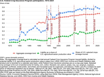
Existing sources of exogenous variation for the identification of crop insurance outcomes in the context of the US fall under four broad categories. The first relies on national-level legislative events driving structural changes in FCIP (Schoengold et al. Reference Schoengold, Ding and Headlee2015; Connor and Katchova Reference Connor and Katchova2020; Wang et al. Reference Wang, Rejesus and Aglasan2021). This first group of instruments proposed by Schoengold et al. (Reference Schoengold, Ding and Headlee2015) takes on a value of unity for years within the respective policy periods and zero otherwise. The major changes in the national policy upon which these instruments are based include updates in The Crop Insurance Reform Act of 1994 (Public Law [P.L] 103-354) (conventionally known as “1994 Act”), The Agricultural Risk Protection Act of 2000 (P.L 106-224) (“ARPA”), The Food, Conservation, and Energy Act of 2008 (P.L 110-246) (“2008 farm bill”), and The Agricultural Act of 2014 (P.L 113-79) (“2014 farm bill”). Notable changes in the 1994 Act were (1) the requirement of producer enrollment in crop insurance as an eligibility criterion for the support provided by certain federal farm support programs; (2) the creation of catastrophic coverage option (CAT) which offers protection of 50% on yield and 60% of expected price all at 100% premium subsidy but with an administrative fee of 50 $/crop/county; (3) the increment of coverage options above CAT; and (4) the authorization of revenue protection products. The ARPA expanded the geographic availability, removed restrictions on livestock products, expanded private sector product development, and authorized premium reduction plans that allow approved insurance providers (AIPs) to offer reduced premiums, thereby improving their competitive advantage. The 2008 farm bill eliminated the premium reduction plans enacted by ARPA, reduced premium subsidies for area plans, and increased CAT fees from 50 to 300 $/crop/county. The 2014 farm bill also expanded the program by authorizing higher coverage levels with lower deductibles and introduced new products aimed at shallow loss coverage (e.g., Supplemental Coverage Option and Stacked Income Protection), providing producers the option to exclude low yields from their production history under certain circumstances, linked premium subsidy eligibility to conservation compliance, and premium subsidy reduction to planting on native sod in some states. Figure 1, retrieved from Economic Research Service [ERS] (2022), shows that these legislative changes improved crop insurance participation.

Figure 1.

US Federal Crop Insurance program participation improved with legislation.

The second set of instruments first introduced by Yu et al. (Reference Yu, Smith and Sumner2018) is based on policy changes to the suite of subsidy rates. Yu et al. (Reference Yu, Smith and Sumner2018) argue that changes in legislation create a structural break that shifts the suite of subsidy rates exogenously in a way that is not driven by endogenous factors related to crop production. These instruments used by Yu et al. (Reference Yu, Smith and Sumner2018) are generated by dividing the annual subsidies for yield and revenue protection policies for a given coverage level and dividing this by the sum of their associated total premiums. Yu et al. (Reference Yu, Smith and Sumner2018) recommended the 65% and 75% coverage levels as the point of aggregation since they are the most patronized and observations exist for all years; thus, two sets of variables are developed and used as the instruments. Even though instruments by Yu et al. (Reference Yu, Smith and Sumner2018) are also based on one-time changes in legislation, unlike the first they are scalar. Thus, they can capture exogenous changes in legislation, and hence crop insurance outcomes, beyond the initial year of passage of the associated law.

The first and second sets of instruments all rely on crop insurance legislation set at the national level. Thus, even though they can account for within-county variation in crop insurance outcomes over time, they do not provide the spatial (between-county) variation necessary for proper instrumentation in a cross-sectional setting. The third set of instruments overcomes this by using a measure of the degree to which crop insurance legislation affects a county. First introduced by DeLay (Reference DeLay2019), these instruments are based on a measure of preferences for different types of insurance before the enactment of legislative changes discussed above. Particularly, these instruments are generated by interacting a policy exposure measure with dummy variables representing each of the four policy change periods (essentially the first set of instruments). In their application, DeLay (Reference DeLay2019) used total insured acres divided by total cropland as the policy exposure measure. Total acres for each period were taken as reported in the associated latest Census of Agriculture survey. According to DeLay (Reference DeLay2019), the instrument captures how much a county sees its effective subsidy rates increase and hence can be used to estimate the variation in insured acreage due only to changes in government policy and not to contemporaneous land-use decisions. Connor et al. (Reference Connor, Rejesus and Yasar2021) adopted a version of this instrument that used a policy exposure measure constructed as the proportion of insured acres for coverage levels.

The final set of instruments, upon which this study is based, relies on the current rating framework used by RMA (i.e., continuous rating). The main idea is that FCIP premium rates are determined via exogenously set rating parameters, and hence, the parameters if known can be used to generate exogenous variation in premium rates that producers face when making crop insurance decisions. To the best of our knowledge, Woodard and Yi (Reference Woodard and Yi2020) and Tsiboe and Turner (Reference Tsiboe and Turner2022) are the only studies relying on this strategy. According to Tsiboe and Turner (Reference Tsiboe and Turner2022), even though information on producers that participated in the FCIP in the past is used in the determination of the policy variables, it is unlikely that the information from a single producer will influence their outcome in such a way that will be advantageous to them in the current season. Particularly, previous yields reported by producers contribute to a producer’s historical loss experience but are fixed and not under the control of producers once reported. Accordingly, FCIP premium rates can be thought of as sequentially exogenous to producer insurance decisions. This assumption is plausible because the rating parameters are finalized a season or two in advance. Consequently, the exogenous portion of FCIP premium rates is driven by the rating parameter and the endogenous portion by the insured’s choice of insurance unit, coverage level, and their historic production experience.Footnote ⁴

Although Woodard and Yi (Reference Woodard and Yi2020) and Tsiboe and Turner (Reference Tsiboe and Turner2022) use a similar methodology of approximating rating parameters, a few nuanced differences persist. Given the form of the continuous rating formula, Woodard and Yi (Reference Woodard and Yi2020) estimated the rating parameters from a latent rate curve using observed loss experience data via a regression framework.Footnote ⁵ According to Tsiboe and Turner (Reference Tsiboe and Turner2022), estimating the rating parameters from the loss experience data including the year for which they were set does not make them entirely void of endogeneity problems. Alternatively, Tsiboe and Turner (Reference Tsiboe and Turner2022) essentially take the rating parameters as given (i.e., the same parameters farmers faced when they made the decisions leading to the loss experience data), under the presumption that this approach makes their instrument less likely to be afflicted by the same source of previously described simultaneity bias.

In this study, we aim to improve the identification of crop insurance for both temporal and spatial settings. Currently, an instrument based on structural dummy variables (Schoengold et al. Reference Schoengold, Ding and Headlee2015) and those based on national-level subsidy rates (Yu et al. Reference Yu, Smith and Sumner2018) lack the needed variation for applications in a cross-sectional setting. On the other hand, those (Woodard and Yi Reference Woodard and Yi2020; DeLay Reference DeLay2019) using instruments based on loss experience outcomes including the year of the study introduce new sources of bias that likely makes these alternative instruments not entirely void of the same endogeneity problems they hope to address. Neither Woodard and Yi (Reference Woodard and Yi2020) and Tsiboe and Turner (Reference Tsiboe and Turner2022) guide how to arrive at premium rating-based instruments for years before 2000. While Tsiboe and Turner (Reference Tsiboe and Turner2022)’s approach most closely reflects reality, it is only relevant for years after 2000 when the rating method upon which their instruments are based was in effect.Footnote ⁶ Currently, the rating parameters from 2011 to 2023 are available in easily accessible files via RMA’s Actuarial Data Master (ADM) data set, but those from 2001 to 2010 are not easily accessible.Footnote ⁷ Additionally, since the continuous rating was not in existence pre-2001 there are no existing values for rating parameters for most of the FCIP historical time series data. However, as will be shown, some of the continuous rating parameters (specifically the base rate reflecting the county reference rate and catastrophic fixed loading factor) can be approximated using historical data.

Premium rating system

The system for rating crop insurance contracts within the FCIP, which is based on a principle known as loss-cost ratio (LCR) rate-making, is understandably very complex (see for example K. H. Coble et al. (Reference Coble, Knight, Goodwin, Miller, Rejesus and Duffield2010) and K. Coble et al. (Reference Coble, Goodwin, Miller, Rejesus, Harri and Linton2020)). This section attempts to provide a simplified overview of FCIP contract rating as it relates to this study. Focus is given to individual-level yield protection policies, but the discussion that follows can be applied to other policy types. By extension, output price is assumed to be equal to unity without loss of generality.

Individual-level yield insurance contracts have eight main components: rate yield ( $\bar y$ ), approved yield ( $\ddot y$ ), coverage level ( $\theta $ ), indemnity ( $I\left( y \right)$ ), premium rate ( $\tau $ ), premium ( $P$ ), and subsidy ( $S\left( {\theta ,u} \right)$ ). Rate and approved yields are essentially the averages of actual production history (APH) reported by farmers with the main difference being that the latter is adjusted upward via several aspects of RMA’s actuarial process (e.g., yield exclusion, yield substitution, and trend adjustments).Footnote ⁸ For a given contract, the producer can choose to insure their approved yield at a coverage level of $\theta $ with a respective yield guarantee of $\theta \ddot y$ . Thus, the per-acre indemnity for a given yield outcome, $y$ , is given by $I\left( y \right) = {\rm{\;}}max\left[ {0,\theta \ddot y - y} \right]$ .

In the U.S., FCIP premium rates are required to be set such that the resulting policies are actuarially fair; meaning premiums are set equal to expected per-acre indemnities. Standardizing expected per-acre indemnities by insured liability can be characterized by the following equation.

(1) $$\tau \left( \theta \right) = {{E\left[ {I\left( y \right)} \right]} \over {\theta \ddot y}} = {1 \over {\theta \ddot y}}\mathop \int \nolimits_0^{\theta \ddot y} \left( {\theta \ddot y - y} \right)f\left( y \right)dy$$

where $f\left( y \right)$ is the probability density function of $y$ . Since indemnities are stochastic and not known at the time the policy is written, crop insurance policies are typically generated under the assumption that $f\left( y \right)$ is conditional on an adjustment mechanism that relies on the underlying risk profile of the producer seeking insurance. This risk profile is not observable and is approximated by the productivity of the producer seeking insurance relative to their peers. The magnitude of this adjustment is determined using RMA’s “continuous rating formula” (Milliman and Robertson 2000; Risk Management Agency [RMA] 2000, 2009).

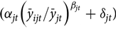
The default form of the continuous rating formula is specified according to the following equation

(2) $${\tau _{ijt}} = \left[ {{\alpha _{jt}}{{\left( {{{\bar y}_{ijt}}/{{\bar y}_{jt}}} \right)}^{{\beta _{jt}}}} + {\delta _{cjt}}} \right]\vartheta \left( {{\theta _{ijt}},{u_{ijt}}} \right)$$

where the subscript $ijt$ represents an insured ( $i$ ) seeking protection defined by an insurance pool ( $j$ ) for crop year $t$ .Footnote ⁹ The parameters ${\alpha _{jt}}$ and ${\delta _{jt}}$ , respectively, represent the reference rate and catastrophic fixed loading factor for a common coverage level (conventionally at the 65% level) for the insurance pool. In what follows, the continuous rating formula is used to adjust the common coverage level rate for the insurance pool based on the specific risk and choices of the producer seeking insurance. These mechanisms are analogous to how other property and casualty insurance rate factors are developed from a combination of experience and differential exposure information (Sherrick et al. Reference Sherrick, Schnitkey and Woodward2014).

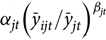
The first step in calculating rates for a given producer is to adjust the reference rate based on the assumption that historical yield and risk are correlated. This adjustment is represented in equation (3) by ${\left( {{{\bar y}_{ijt}}/{{\bar y}_{jt}}} \right)^{{\beta _{jt}}}}$ which is the ratio of a given producer’s historic mean yield, ${\bar y_{ijt}}$ , divided by a reference yield ( ${\bar y_{jt}}$ ) of the insurance pool in which they are rated, raised to a power, ${\beta _{jt}}$ , known as the continuous rating exponent. The continuous rating exponent takes on a negative value which assumes that higher production levels correlate with less risk. This means that when a producer’s historical mean yield is greater than the county reference yield (i.e., ${\bar y_{ijt}}/{\bar y_{jt}} \gt 1$ ), the county reference rate is adjusted downward for that producer.Footnote ¹⁰ The next step in determining a producer’s premium rate is to adjust their initial rate, ${\alpha _{jt}}{\left( {{{\bar y}_{ijt}}/{{\bar y}_{jt}}} \right)^{{\beta _{jt}}}}$ + δ_jt, via a scaling function, $\vartheta \left( \cdot \right)$ , which is based on the producer’s choice of coverage level ( ${\theta _{ijt}}$ ) and insurance unit election ( ${u_{ijt}}$ ).Footnote ¹¹

The total price of the insurance contract, $P$ , is set equal to the product of the premium rate, $\tau \left(. \right)$ , and the yield guarantee, $\theta \ddot y$ , such that $P = \tau \left(. \right)\theta \ddot y$ . The final price paid by the insured is subsidized at a rate $S\left( {\theta ,u} \right)$ that is tied to coverage level and insurance unit and not to location or the crop. RMA internally sets the values for the parameters ( $\alpha ,\delta ,\beta $ , and ${\bar y_c}$ ) in the continuous rating formula using historical loss data from the FCIP coupled with empirical approaches originating in the early 1980s (Sherrick et al. Reference Sherrick, Schnitkey and Woodward2014). Thus, because coverage in the 1980s was limited to only 65% for yield protection, the rating system harmonizes all historical contracts to a 65% coverage on yield. Given the harmonized data, the reference rate ( $\alpha $ ) for an insurance pool is determined as the annual mean of the pool’s historical LCR which is capped to limit the influence of outliers from anomalous catastrophic loss events (K. H. Coble et al. Reference Coble, Knight, Goodwin, Miller, Rejesus and Duffield2010). The excess exposure resulting from the capped LCR is then used to determine the catastrophic fixed loading factor ( $\delta $ ). According to the literature, the pool’s reference yield ( ${\bar y_c}$ ) is determined as the ten-year average of the yield of the insurance pool (Rejesus et al. Reference Rejesus, Goodwin, Coble and Knight2010), and the continuous rating exponent ( $\beta $ ) is estimated by regressing LCR on ${\bar y_{ijt}}/{\bar y_{jt}}$ using farm-level data (Tsiboe and Tack Reference Tsiboe and Tack2022).

From the foregoing discussion, the exogenous portion of FCIP premium rates ( $\tau \left( {\theta ,u,\bar y;\omega } \right)$ ) is driven by the policy parameter space $\omega \in \left\{ {\alpha ,\beta ,\delta ,{{\bar y}_c}} \right\}$ and the endogenous portion by the insured’s choice of insurance unit $\left( u \right)$ , coverage level $\left( \theta \right)$ , and their historic production experience $\bar y$ . In what follows, we outline how a target rate reflecting the county reference rate ( $\alpha $ ) and catastrophic fixed loading factor ( $\delta $ ) can be approximated using historical data.

Deriving crop insurance rating parameters

It is worth stressing here that our goal is not to provide alternative rating procedures but to illustrate how key parameters in current individual policy rating could be approximated for instrumental variable purposes. Several third-party FCIP reports on crop insurance rating methodology are of interest to this study which is used to draw insights to generate target rates that are comparable to county reference rates and catastrophic fixed loading factors under the continuous rating framework. We primarily draw from the RMA-commissioned review of the APH and COMBO rating methods (K. H. Coble et al. Reference Coble, Knight, Goodwin, Miller, Rejesus and Duffield2010). For this study, the FCIP has publicly available historic loss experience data from 1948 to 2021 (i.e., 74 years of data) of which data from 1961 to 2020 (i.e., 60 years of data) are relevant for this study.

This study first defines an aggregation unit characterized by a cross-sectional index i (e.g., county-crop, county, state, etc.) and time index t (e.g., year) for which an approximation of a target rate ( ${\tau _{it}}$ ) is desired. The stochastic historic empirical LCR is denoted as $\left\{ {LC{R_{it - s}}} \right\}_{s = 2}^T$ , where $LC{R_{it}} = min\left( {1,max\left[ {0,indemit{y_{it}} \div liabilit{y_{it}}} \right]} \right)$ .Footnote ¹² For each aggregation unit, the LCR reflects the proportion of insured liability that was paid to producers each year, that is, the return on insurance. In practice, RMA first adjusts both historic liabilities and indemnities to a common coverage level (conventionally at the 65% level) and harmonizes all contracts to yield-based protection before taking this ratio. However, since the objective is to estimate target rates over the entire history of the FCIP, this study forgoes these adjustments because historic coverage level choice data before 1989, and the price data needed to convert all contracts to yield-based protection are currently not available in the public domain.

The timing of actuarial releases by RMA suggests that rating parameters are derived two years ahead of a given crop year; thus, the historic empirical LCR series for a given cross-sectional index end at $t - 2$ . Given $\left\{ {LC{R_{it - s}}} \right\}_{s = 2}^T$ , an empirical burn rate ( ${\bar \tau _{it,BR}}$ ) is estimated as the mean of the series. Next, the burn rate is loaded (by dividing by 0.88) to obtain the raw rate ( ${\bar \tau _{it,RR}}$ ). The underlying data for rating crop insurance (i.e., LCRs) are often highly variable. Thus, the RMA rate-making process includes several steps intended to smooth some of these fluctuations to prevent outsized influence from a singular data point. One such process is a spatial smoothing procedure that takes a weighted average of the raw rate and surrounding raw rates (i.e., county group rate) to determine a final rate. This study applies a similar strategy where a county group rate ( ${\bar \tau _{it,CR}}$ ) is defined as the weighted average (by the sum of the liability for periods less than $t - 2$ ) of the raw rates of all adjoining counties. The final target rate which can be used as an instrument is then taken as ${\tau _{it}} = 0.6{\bar \tau _{it,RR}} + 0.4{\bar \tau _{it,CR}}$ , where the weighting values of 0.6 and 0.4 are based on past RMA practices (K. H. Coble et al. Reference Coble, Knight, Goodwin, Miller, Rejesus and Duffield2010).Footnote ¹³

The resulting target rate, ${\tau _{it}},$ is slightly different than any existing RMA premium rating parameters but performs a similar function of explaining variation in lost cost ratios (this is validated empirically in a later section). Thus, ${\tau _{it}}$ is analogous to the exogenous parameters from equation (2) in the sense that ${\tau _{it}}$ is exogenous to any producer insurance decisions and is also correlated with final premium rates by being derived with the purpose of empirically fitting historical lost cost ratio data. However, ${\tau _{it}},$ has the benefit of being derivable for any spatiotemporal setting from publicly available data, making it a more accessible instrument relative to other potential rating parameter-based instruments. More specifically, ${\tau _{it}}$ , approximates RMA’s initial rate, (defined in equation (3) as $({\alpha _{jt}}{\left( {{{\bar y}_{ijt}}/{{\bar y}_{jt}}} \right)^{{\beta _{jt}}}} + {\delta _{jt}})$ for the special case where the producer’s mean yield, ${\bar y_{ijt}}$ , is exactly equal to the reference yield, ${\bar y_{jt}}.$ In other words, ${\tau _{it}}$ reduces to an approximation of ${\alpha _{jt}} + {\delta _{jt}}$ which tracks variation in premium rates without the influence of the endogenous portions of the continuous rating formula.

Data and construction of relevant variables

Primary FCIP information for the construction of the target rate which can be used as an instrument was retrieved from RMA’s summary of business and cause of loss files. RMA provides three different versions of the summary of business which are aggregated by:

1. (1) State/County/Crop,

2. (2) State/County/Crop/Coverage, and

3. (3) State/County/Crop/Coverage/Type/Practice/Unit Structure.

For the cause of loss, RMA provides three different versions:

1. (1) Summary of Business with Month of Loss,

2. (2) Indemnities Only, and

3. (3) Indemnities with Month of Loss.

We use information from all six sources to construct a county-crop panel data set from 1948 to 2020 that includes FCIP loss experience information on liability insured by producers, total premium, premium subsidy, and indemnity paid to farmers. The procedure used to aggregate the information from all six sources first sums up the variables of interest for each county-crop-year combination, separately for each of the six data sources. Then for each county-crop-year combination, the maximum among the six data sources is used as the representative value for each variable. The rationale for doing this is that RMA periodically updates the summary of business and cause of loss files as new information, which is continuously provided by AIPs, becomes available. This means any given data set for a particular year continues to receive minor changes for some time after that particular year has ended. Thus, there will sometimes be differences in the same metric across different file sources, but presumably, the metrics tracked in these sources, such as policies sold, are monotonically increasing over time meaning the maximum value from all available data sources should be the most reflective of reality.

In addition to this data, the study also retrieved actuarial information (i.e., actual values for the county base rates) from RMA’s ADM spanning from 2011 to 2020.Footnote ¹⁴ The specific data retrieved from the ADM include the county reference rate and catastrophic fixed loading factor. For each county-crop-year, the RMA-set county reference rate and catastrophic fixed loading factor were taken as the mean of all the respective values retrieved from RMA’s ADM that could be associated with that county-crop-year combination. Finally, a representative target rate comparable to those generated from this study was taken as the sum of the county reference rate and catastrophic fixed loading factor.

Table 1 shows the descriptive statistics of the data used for the approximation of target rates. The sample is composed of 564,340 observations with 26,078 unique county-crop FCIP programs. On average, an FCIP county-crop program in the data had an annual insured liability of $3.5 Million on about 15 thousand acres. Total collected premiums for a county-crop program averaged $309,000 of which $91,000 was paid for by government subsidies. The annual mean LCR for FCIP county-crop program from 1948 to 2020 is estimated at 0.12 indicating that for every dollar of liability insured, about 12 cents was paid to farmers to indemnify their losses.

Table 1.

Means and standard deviations of selected variables on US Federal Crop Insurance county-crop programs (1948–2020)

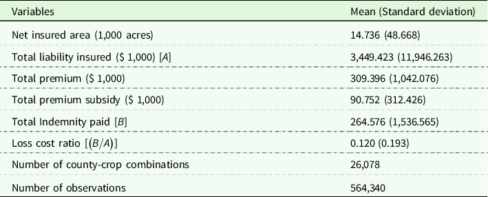
Note: The data was constructed by the authors using primary data from the Risk Management Agency’s summary of business and cause of loss files.

Lost cost ratio predictive performance

The RMA’s rate-making procedures are intended to allow for the estimation of the expected loss component of rates, represented by the LCR (K. H. Coble et al. Reference Coble, Knight, Goodwin, Miller, Rejesus and Duffield2010). Thus, the approximation of the target rate proposed by this study should be able to predict LCRs to a similar degree of accuracy compared to the status quo methods used by RMA. In that regard, this study evaluates the LCR predictive performance of all the various rates estimated in the approximation procedure by using both out-sample (via five-fold-cross-validation) and in-sample prediction performance. Both measures are operationalized on an annual basis from 2011 to 2020 and are evaluated in terms of the LCR prediction error (mean squared error) generated in this study relative to the mean error when actual observed rates set by RMA are used to predict the LCR. Thus, values below one are preferred with values significantly larger than 1 indicating worse performance over LCR predictability.

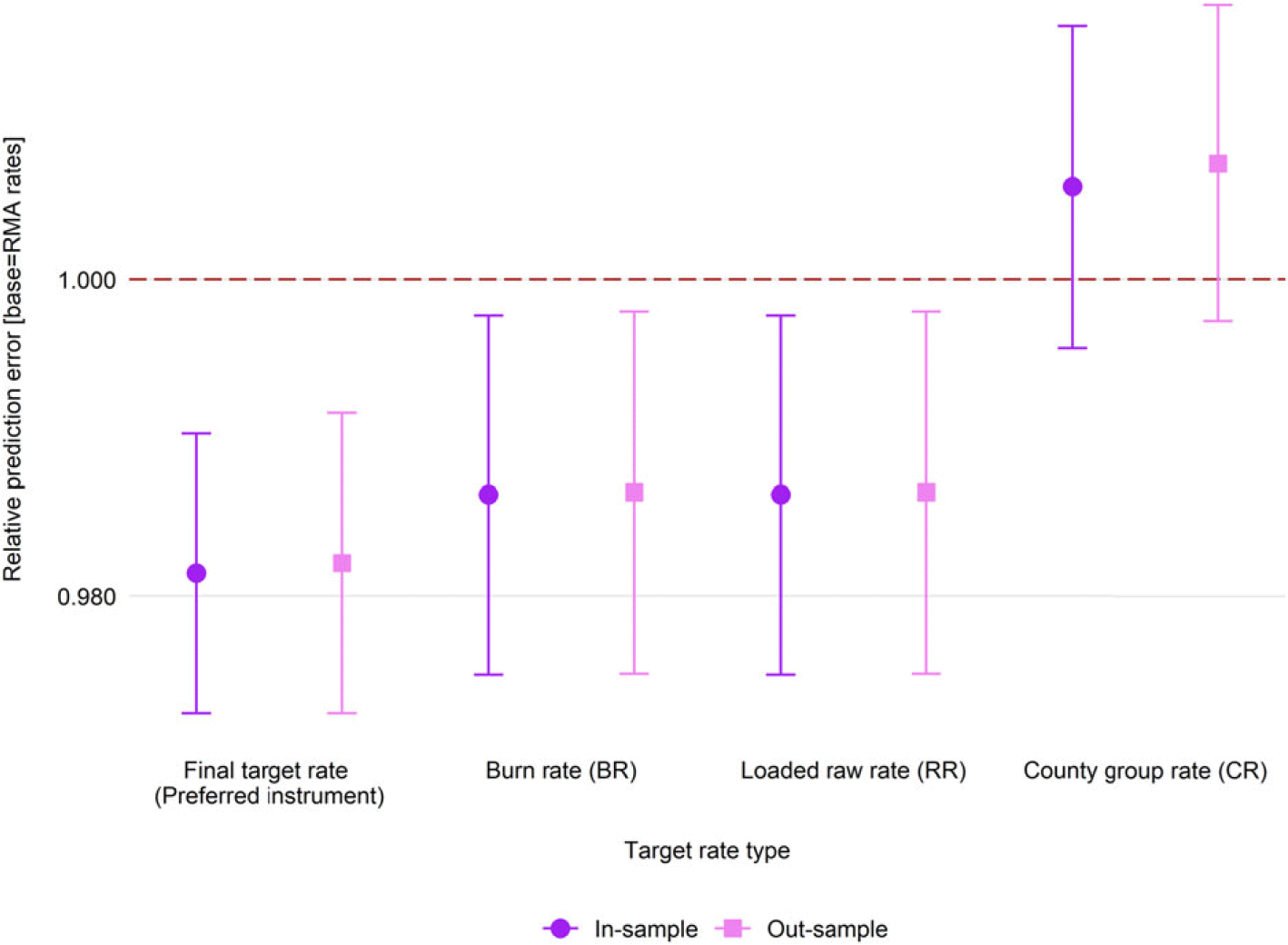
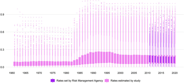
Figure 2 shows that the final target rate estimated in the approximation procedure reflects expected losses better than the burn rates, raw rate, and county group rate. Model diagnostics (shown in Figure S1) also indicate that the final target rate performs slightly better in terms of R-squared, AIC, and BIC. Figure 3 shows box plots of the final target rate and the official rates produced by RMA. As can be seen in the figure, the approximation proposed in this study yields target rate distributions that are quite close to the target rate distributions produced by RMA for the years 2011–2020.Footnote ¹⁵

Figure 2.

Loss cost ratio predictive performance of different rate approximation methods.

Notes: Graph shows the in- and out-sample loss-cost ratio predictive performance of various approximations of USDA Risk Management Agency (RMA) crop insurance target rates (i.e., the sum of county reference rate and catastrophic fixed loading factor). The values are evaluated in terms of relative performance to the mean of RMA target rates for 2011–2020.

Figure 3.

County-crop approximated target rate distribution by crop year.

Notes: Graph shows the distribution of USDA Risk Management Agency (RMA) crop insurance target rates (i.e., the sum of county reference rate and catastrophic fixed loading factor) and its preferred approximation from the stud.

Empirical application

As was discussed in the introduction, several sources of endogeneity are of concern in empirical studies making use of crop insurance demand as either an independent or dependent variable. What follows are two sets of empirical examples of how to address these endogeneity concerns by using derived rating parameters as instrumental variables. The primary goal of the empirical examples is not to provide a detailed analysis of the underlying issues but to illustrate how the target rates approximated in this study could be used to deal with endogeneity as it relates to the context of this paper. The examples can easily be generalized to other applications and research settings that make use of direct crop insurance outcomes like participation and premiums as independent variables.

Empirical application: crop insurance demand as a function of premiums

This first set of empirical applications exemplifies the use of the derived instrument to address the situation where the total premium for crop insurance is an independent variable of interest. Past studies try to circumvent the endogeneity problem in modeling crop insurance demand by using Heckman-type models of participation (Goodwin and Kastens Reference Goodwin and Kastens1993; Richards Reference Richards2000; Shaik et al. Reference Shaik, Coble, Knight, Baquet and Patrick2008). Unfortunately, the majority of existing studies do not consider this endogeneity problem (Gardner and Kramer Reference Gardner, Kramer, Hazell, Pomareda and Valdes1986; Hojjati and Bockstael Reference Hojjati, Bockstael and Harry1988; Barnett et al. Reference Barnett, Skees and Hourigan1990; Calvin Reference Calvin1990; Goodwin Reference Goodwin1993; Goodwin and Kastens Reference Goodwin and Kastens1993; K. H. Coble et al. Reference Coble, Knight, Pope and Williams1996; Yi et al. Reference Yi, Bryant and Richardson2020; Bulut and Hennessy Reference Bulut and Hennessy2021). Thus, empirical approaches seeking to econometrically identify FCIP demand elasticities, which do not explicitly account for this source of endogeneity, are suspect from a causal perspective. Here, county-level corn production data are used to estimate the responsiveness of crop insurance demand to premium rates at both the intensive and extensive margins.

Crop insurance data for corn from 1975 to 2020 used in this application are obtained from the same data sources used in approximating the target rates. Specifically, the variables of interest include the total potential liability, total insured liability, total premium, and total subsidy for corn in county i for crop year t.Footnote ¹⁶ Data on planted acres of corn were also retrieved from NASS Quick Stats, and where missing, the planted acres were filled in with harvested acres which were also obtained from the same source. Using this data, several variables of interest were calculated; the aggregate coverage level ( ${\theta _{it}}$ ) as total insured liability divided by total potential liability; premium per dollar of liability ( ${r_{it}}$ ) as the total premium divided by total insured liability; and subsidy per dollar of premium ( ${s_{it}}$ ) as the total premium subsidy paid divided by the total premium. Finally, this study used the same corn price discovery method employed by RMA in estimating projected prices to approximate state-level expected prices for corn from 1975 to 2020. Table S1 shows the descriptive statistics of all variables used in this empirical application.

The empirical model is formulated as

(4) $$\ln {\theta _{it}} = {\beta _0}{ + _\tau }\ln {r_{it}} + {\beta _s}\ln {s_{it}} + {\beta _w}{w_{it}} + {v_{it}} + {\varepsilon _{it}}$$

where the variable ${\theta _{it}}$ is a measure of crop insurance uptake at both the intensive margin and extensive margin (A second version of this model is also specified to explain demand exclusively at the extensive margin by setting ${\theta _{it}}$ equal to the share of eligible acres enrolled in crop insurance as the dependent variable).Footnote ¹⁷ The vector ${w_{it}}$ contains the log expected price, log planted acres, and state-specific time trends. The terms ${v_{it}}$ and ${\varepsilon _{it}}$ are county fixed effects (FE) and error terms, respectively. The error terms are assumed to have an expected value of 0 but can be heteroskedastic so standard errors are clustered by the county to allow for ${\varepsilon _{\;it}}$ to be spatially correlated within each crop year (Petersen Reference Petersen2009; Cameron et al. Reference Cameron, Gelbach and Miller2011; Thompson Reference Thompson2011).

The premium per dollar of liability ( ${r_{it}}$ ) in equation (4) is the weighted average of farm-level FCIP premium rates represented by equation (2). As noted in previous sections, FCIP premium rates are driven by both exogenous and endogenous factors, which makes them potentially endogenous to crop insurance demand. For example, a corn farmer with a high-risk profile will end up paying a higher premium compared to a lower-risk farmer. At the same time, farmers tend to allocate fewer corn acres in a county characterized by a greater risk profile, ceteris paribus (Hojjati and Bockstael Reference Hojjati, Bockstael and Harry1988). Alternatively, corn growers in counties that have a high-risk profile for corn production are likely to increase their crop insurance coverage. In these cases, estimating the empirical model via ordinary least squares (OLS) will result in biased coefficient estimates since “risk” is an omitted independent variable that partially determines crop insurance coverage and is correlated with the premium per dollar of liability. The identification strategy in this empirical application is to utilize the exogenous RMA-set variations in continuous rating formula policy parameters to generate exogenous variation in premium per dollar of liability via instrumental variables estimation. However, since these parameters are not publicly available for the entire period under review (1975–2020), the empirical application uses a comparable approximation of the sum of county reference rate and catastrophic fixed loading factor as outlined in previous sections. In this setting, the aggregation unit to generate the instrument (i.e., the final target rate) is characterized by a cross-sectional index defined as the unique combination of county crops in the underlying data for the analysis.

Table 2 reports the estimated results for Equation (4) using the combined measure of demand at the intensive and extensive margins. Columns (1) and (2) report the estimation results based on two-staged least squares (2SLS) regression with and without FE, respectively. Similarly, columns (3) and (4) report OLS results with and without FE, respectively. The Anderson-Rubin chi-sq test for exogeneity of premium per dollar of liability ( ${r_{it}}$ ) is rejected (p < 0.01) for both 2SLS models, suggesting that the previously described concerns over endogeneity are valid and that an instrumental variables approach is appropriate. The question that remains is if the approximated target rates are strong enough to aid in identifying the causal effect of premium rates on crop insurance demand. First-stage F-statistics are well above the thresholds suggested by Stock and Yogo (Reference Stock and Yogo2005) indicating that the final target rate is not a weak instruments.

Table 2.

Crop insurance demand for corn production in the US for 1989–2020 at The intensive margin is inelastic to changes in premiums rates

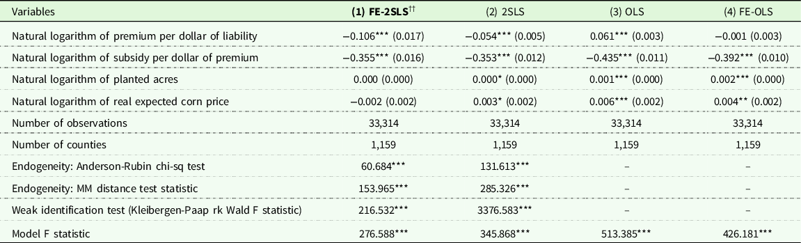
Notes: The outcome variable is county-level corn crop insurance demand at the intensive margin is measured as the total liability divided by the total potential liability implied by those who purchased corn crop insurance in that county. The data used was constructed by the authors using primary data from (1) Risk Management Agency’s summary of business and cause of loss files. The preferred model is ††.Significance levels – *p < 0.1 **p < 0.05, ***p < 0.01. Standard errors in parentheses are clustered by county.

Generally, Table 2 shows that the preferred model [Model 1: FE-2SLS] has estimated coefficients that are varied in direction and larger in magnitude than the model without instrumental variables (IVs) [Model 3 and 4: OLS and FE-OLS] or without FE [Model 2: 2SLS] suggesting that either crop insurance choices or time-varying unobserved individual risk profiles bias the responsiveness of crop insurance demand.

Table 3 reports estimated results for Equation (4) as specified to represent demand exclusively at the extensive margin and yields qualitatively similar results when compared to Table 2. The Anderson-Rubin chi-sq test is rejected (p < 0.01) for the 2SLS model making use of fixed effects (although this is not the case if fixed effects are excluded). Weak instruments are again not a problem in this specification with both 2SLS models exhibiting first-stage F-stats that are well above conventionally set thresholds. Again, the preferred model [Model 1: FE-2SLS] yields a coefficient on the premium per dollar of liability that is opposite in sign and larger in magnitude compared to the OLS models in Table 3.

Table 3.

Crop insurance demand for corn production in the US for 1948–2020 at The extensive margin is inelastic to changes in premiums rates

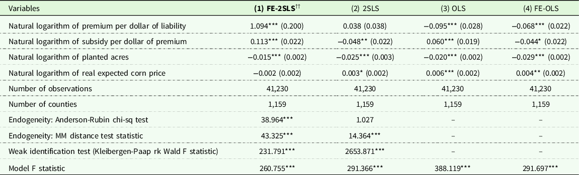
Notes: The outcome variable is county-level corn crop insurance demand at the extensive margin measured as the total insured acres for corn divided by the total planted of corn in that county. The data used was constructed by the authors using primary data from (1) Risk Management Agency’s summary of business and cause of loss files, and (2) NASS Quick Stats. The preferred model is ††.Significance levels – *p < 0.1 **p < 0.05, ***p < 0.01. Standard errors in parentheses are clustered by county.

Concerning the effect that subsidies have on demand for insurance, Table 2 suggests a negative effect while Table 3 suggests a positive relationship between increasing subsidies per dollar of premium and demand at the extensive margin. This could be interpreted as evidence that increasing subsidy rates induce a trade-off between demand at the intensive margin in favor of increased demand at the extensive margin. However, as noted previously, this analysis is not intended to be a comprehensive analysis of demand for crop insurance, but instead serve as a demonstration of the validity of the proposed instrumental variable.

Empirical application: farm debt as a function of crop insurance participation

The second set of empirical applications demonstrates how to instrument for measures of crop insurance demand that appear as independent variables of interest but remain endogenous with respect to the outcome of interest. This example is based on existing work assessing the role that crop insurance has on farm debt use (Ifft et al. Reference Ifft, Kuethe and Morehart2015) and demonstrates that the proposed instrument also has favorable diagnostics when demand for insurance appears as an endogenous independent variable.

Both theoretical and empirical research on risk balancing has shown that producers could increase financial risk in response to a decline in business risk. By extension, this also means that farm policy programs like the FCIP that decrease business risk could have causal impacts on financial risk levels. However, producers’ decisions on coverage through crop insurance and farm debt are likely influenced by the same unobservables, and thus endogenous. Ifft et al. (Reference Ifft, Kuethe and Morehart2015) account for this simultaneity bias in their estimation of the difference in debt use attributable to FCIP via two methods: (1) propensity score matching (to approximate a controlled experiment) and (2) seemingly unrelated regression (to explicitly model joint determination of farm debt structure and crop insurance participation). In this example, we provide another way to use the final target rate in this paper under an instrumental variable regression framework.

Like Ifft et al. (Reference Ifft, Kuethe and Morehart2015), we use data from the nationally representative Agricultural Resource Management Survey (ARMS), with the key exception that the sample is pooled for the ARMS fielded from 2011 to 2020.Footnote ¹⁸ We follow Ifft et al. (Reference Ifft, Kuethe and Morehart2015) by limiting the sample to farm businesses as defined officially by USDA, which includes (1) farms where the principal operator’s primary occupation is farming, (2) farms with sales over $250,000, and/or (3) non-family farms.

The empirical model is formulated as

(5) $${\rm{asinh}}\ {D_i} = {\beta _0} + {\beta _\tau }\ {\rm{asinh}}\ {E_i} + {\beta _z}{z_i} + {\mu _i}$$

where the variable ${D_i}$ is a measure of debt use which, following Ifft et al. (Reference Ifft, Kuethe and Morehart2015), is defined as one of (1) total farm financial debt; (2) non-real estate financial debt; (3) real estate financial debt; (4) short-term financial debt (outstanding); (5) short-term financial debt (all); (6) farm business debt to asset ratio; (7) share of short-term financial debt (all) to total operating expenses; and (8) current ratio, all in per-acre terms. The key independent variable is crop insurance participation measured by the total per-acre premium paid by the farm ( ${E_i}$ ). This is the only reasonable scalar measure of FCIP participation in the ARMS data as it has been shown that the key function that determines the premium paid by insured is increasingly convex in coverage (Woodard and Yi Reference Woodard and Yi2020). The vector ${z_i}$ contains control variables and is defined, again based on (Ifft et al. Reference Ifft, Kuethe and Morehart2015), to include operators’ age and education; total operating acres; percent of cropland; unit structure; sales class as defined by USDA; ERS Farm Resource Region; and an annual trend variable. Because some of the debt-use decision outcome variables contain zero and non-positive values, we used the Inverse hyperbolic sine transformation ( ${\rm{asinh}}$ ). Likewise, the total premium paid by farmers also has zero values for non-participating farms. After the estimation of Equation (5), we used procedures outlined in the literature to approximate effects in elasticity terms (Bellemare and Wichman Reference Bellemare and Wichman2020). ARMS is based on a stratified sample design as such it requires weighted estimation of sample statistics; thus, USDA recommended delete-a-group (out of 30 groups) jackknife procedure was used to estimate standard errors. In this setting, the aggregation unit to generate the instrument is characterized by a cross-sectional index defined as the county.

Table 4 provides results for the empirical application focused on estimating farm debt as a function of total crop insurance expenditures. The null is rejected for the Anderson-Rubin test for 6 out of 8 considered debt outcomes suggesting that, in general, the instrumentation is an appropriate choice for this application. For all specifications in Table 4, weak instruments do not appear to be a problem (first-stage F-stats are over 100 for all specifications). Across all models, instrumental variables generally produce large coefficients on crop insurance expenditures relative to OLS results, but with similar or decreased statistical significance. This is potentially a result of the decreased efficiency of two-staged least squares. However, given the favorable diagnostic tests and theoretical basis for endogeneity, two-staged least squares estimates are still preferable to OLS in this empirical application.

Table 4.

Federal Crop Insurance led to higher farm debt use in the US Farm economy from 2011 to 2020

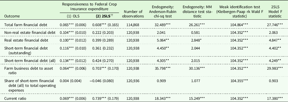
Notes: The farm-level data is from the 2011 to 2020 Agricultural Resource Management Survey (ARMS) Phase 3 data. The preferred model is ††.Significance levels – *p < 0.1 **p < 0.05, ***p < 0.01. Standard errors are calculated using the delete-a-group jackknife.