


1. INTRODUCTION
Most glaciers in the world have retreated significantly during the 20th century, and there is evidence that shrinkage and wastage of ice bodies have accelerated in the last two decades (Marshall, Reference Marshall2014). Glaciers in the Pyrenees are among the most meridional glaciers in Europe (Grunewald and Scheithauer, Reference Grunewald and Scheithauer2010.) and all of them are currently in a critical situation, with clear evidence of very advanced stages of degradation (Rico and others, Reference Rico, Izaguirre, Serrano and López-Moreno2017). According to the results reported by Rico and others (Reference Rico, Izaguirre, Serrano and López-Moreno2017), 33 out of 52 existing glaciers in 1850 (the end of the Little Ice Age, LIA) have already disappeared, 20 of them melted out since 1984. It has implied an 88.25% loss of the glaciated area (−18.18 km2). From 1850 to 1984, glacier area changed from 20.6 to 8.1 km2 (61% surface reduction). In 2016, glacier area was reduced to only 2.42 km2, distributed in 19 glaciers of small size but still exhibiting clear ice motion indicators.
Despite their reduced size, small glaciers such as those existing in the Pyrenees are interesting to study (Dyurgerov and Meier, Reference Dyurgerov and Meier2000). This is because 80% of the glaciers in the world with a surface area <0.5 km2 represent more than 80% of the total number of glaciers in mid- to low-latitude mountain ranges (Fischer and others, Reference Fischer, Huss, Kummert and Hoelzle2016); and they are a relevant component of the cryosphere contributing to landscape formation, local hydrology and sea-level rise (Huss and Fischer, Reference Huss and Fischer2016). In addition, they are highly sensitive geo-indicators of the most recent climatic variations (Grunewald and Scheithauer, Reference Grunewald and Scheithauer2010). However, the response of glacier mass balance to climate fluctuations during their very last stage before disappearing is not fully understood, since there is a positive and negative feedback that has not yet been properly quantified (Carturan and others, Reference Carturan2013; Huss and Fischer, Reference Huss and Fischer2016). In this way, the last glacier remnants are often confined at the most elevated areas, sheltered from radiation and in the most favourable zones for snow accumulation (receiving avalanches or in the leeside of dominant winds) which may slow their response to regional climatic anomalies (DeBeer and Sharp, Reference Debeer and Sharp2009; Carrivick and others, Reference Carrivick2015). Another process that influences the glacier evolution is the thickness of debris cover. This cover usually expands when glaciers’ motion decreases and, depending on its thickness, it causes an acceleration or deceleration of the glacier ice wastage (Brock and others, Reference Brock2010). Finally, the slope of the ice surface tends to increase with glacier shrinkage, and this can negatively impact snow accumulation (López-Moreno and others, Reference López-Moreno2016). Rocky outcrops may appear within the glacier which enhances incoming longwave radiation to the surrounding ice, and frequent ice collapses may occur, associated with many hollows that generally exist between the ice body and the substrate (Fountain and Walder, Reference Fountain and Walder1998), all of these leading to accelerated ice shrinkage and wastage.
An appropriate diagnosis of the condition of a given glacier needs an accurate estimate of remaining ice volume and quantification of ice motion. Additionally, providing evidences of past and recent changes in ice volume allows understanding the evolution of the glacier in previous and present periods of climate change. This information will assist in understanding the response of mass balance to current climatic variability and change. Moreover, geomorphological studies of moraines, as long as they can be accurately dated, will provide useful information on past glacier evolution (Solomina and others, Reference Solomina2016). An array of different techniques allows measurement of the above-mentioned glacier's characteristics. These include traditional ablation stakes for mass balance and surface ice motion, GPS, ground-penetrating radar (GPR), topographic restitution from aerial imageries, optical and radar remote-sensing images, terrestrial and aerial LIDAR (Light Detection and Ranging) and photogrammetry. Their suitability will depend on the contrasted features of the glaciers to be studied. In the case of small glaciers, their reduced size represents an advantage in monitoring the entire ice body but also limits the application of some of these techniques due to the necessity of higher spatial resolution information. The steepness of the slope, the existence of numerous hollows and frequent rockfalls that usually occur in small glaciers also restrict or prevent in situ measurements (Fischer and others, Reference Fischer, Huss, Kummert and Hoelzle2016).
The Monte Perdido Glacier is the third largest glacier in the Pyrenees. Recent significant losses have been reported, both in its glacier surface area (from aerial photographs) and in the elevation of its ice surface. It has been measured by comparing digital elevation model (DEMs) derived from topographic maps from 1981 and 1999 (Julián and Chueca, Reference Julián and Chueca2007), a new DEM obtained in 2010 from airborne LIDAR, and four successive terrestrial laser scanning (TLS) acquisitions obtained near the end of the ablation period (from 2011 to 2014, López-Moreno and others, Reference López-Moreno2016). In the most recent years (from 2014 to present time), laser scans (TLS acquisitions) have also been conducted in late April or early May to better understand the full mass balance of the glacier. There has been one-field campaign conducted on ground-based interferometry radar (ground-based synthetic aperture radar, GB-SAR) to retrieve glacier motion and two GPR surveys to estimate ice thicknesses. This work presents the application of TLS, GB-SAR and GPR techniques to diagnose the current state of the Monte Perdido Glacier and its recent evolution, allowing an in-depth discussion of the applicability of these geomatic techniques for small and highly degraded glaciers.
2. STUDY AREA
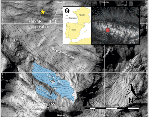
The Monte Perdido Glacier (42°40′50″N; 0°02′15″E) is located in the Central Spanish Pyrenees (Fig. 1). The ice masses are north facing and lie on structural flats beneath the main summit of the Monte Perdido Peak (3355 m) in the Ordesa and Monte Perdido National Park.
Location of the Monte Perdido Glacier, including the scan position for TLS and GB-SAR (coordinates in extended UTM zone 30 T).

Its evolution along the Holocene was determined using 36Cl ages derived from moraines and polished surfaces (García-Ruiz and others, Reference García-Ruiz2014).
Numerous old photographs and the location of the LIA moraines indicate a unique glacier at the foot of the large north-facing wall of Monte Perdido during the LIA (Fig. 1). The ice body was divided into three stepped ice masses connected by serac falls by the mid-20th century, and the lower ice body disappeared during the 1970s (García-Ruiz and others, Reference García-Ruiz2014). The two remaining glacier bodies, which are currently unconnected, are referred to in this paper as the upper and lower Monte Perdido Glaciers. The upper and lower ice bodies have mean elevations of 3110 and 2885 m a.s.l. (Julián and Chueca, Reference Julián and Chueca2007). Despite the high elevation of the upper glacier, snow accumulation is limited due to minimal avalanche activity above the glacier and its marked steepness (≈40°).
According to recent measurements of air temperature (July 2014 to October 2017) at the foot of the glacier (2700 m a.s.l.) and near the summit of the Monte Perdido peak (at 3295 m a.s.l.), the 0°C isotherm is found to lie at 2945 m a.s.l. In an average summer (June to September), the temperature at the foot of the glacier is 7.3°C. No direct observations of precipitation are available at the glacier location, but maximum mean accumulation of snow in late April during the three available years was 3.23 m (see Section 4.1), and average snow density was 454 kg m−3 measured in the field, indicating that total water equivalent during the main accumulation period (October to April) could be close to 1500 mm.
3. METHODS
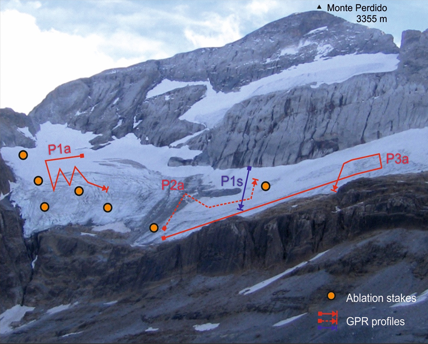
Table 1 shows the field campaigns carried out and considered in this study and the periods when different geomatic and geodetic techniques were developed for the study of Monte Perdido Glacier. In addition to geomatic data, ten ablation stakes were installed in the glacier in 2014; however, three of them were not measured in the following years because the terrain was too steep or crevassed to reach them safely. Location was monitored using RTK GPS for the other seven stakes (Fig. 2), and the information used to obtain annual values of ice speed (see Section 4.2). Ablation stakes were not used to validate TLS ice elevation changes, as the potential uncertainty of TLS data is expected to be lower than the variability of elevation surface changes within the area that some stakes are displaced each year (up to 10 m a−1).
Location of the seven ablation stakes, the profile obtained with GPR in spring 2016 (P1s, in blue) and the three sets of profiles obtained in autumn 2016 (P1a, P2a and P3a, in red) indicating the starting (S) and end (E) points. The photography was taken in 2011. The width of the photo view is ~1 km.
Field campaigns conducted in the glacier during the period 2011–2017
We have also used long-term (1983–2017) meteorological data managed by the Spanish Meteorological Service (AEMET) in a nearby (2.5 km from the glacier) mountain hut (Goriz) at 2250 m a.s.l. that generates temperature (from daily maximum and minimum readings) and precipitation (from daily measurements) anomalies in the study period and places the analysed years in this study in a broader temporal context (López-Moreno and others, Reference López-Moreno2016).
3.1. Terrestrial laser scanner
The use of LIDAR technology, including TLS, has rapidly increased in recent years, and its application has become very frequent for monitoring different aspects of the cryosphere (see the reviews by Deems and others, Reference Deems, Painter and Finnegan2013; Bhardwaj and others, Reference Bhardwaj, Samb, Bhardwaj and Martín-Torres2016). TLS has the advantage of being a mobile device that acquires data at the time and the frequency required by users (compared with airborne acquisitions, which are limited by flight conditions). For this reason, TLS is becoming a popular device to estimate changes in the volume of glaciers, substituting for or complementing the use of traditional estimation of mass balance by ablation stakes (Fischer and others, Reference Fischer, Huss, Kummert and Hoelzle2016).
The device employed in the present study is a long-range TLS (RIEGL LPM-321) that uses time-of-flight technology to measure the time between the emission and detection of a light pulse (at 905 nm, near infrared) from which the distance between the device and the scanned surface is derived. This information allows production of a three-dimensional (3-D) point cloud from real topography. The minimum angular step is 0.0188°, with a laser beam divergence of 0.0468° and a maximum working distance of 6000 m, although there is a considerable loss of accuracy when a range of 3000 m is exceeded (López-Moreno and others, Reference López-Moreno2017).
We used an almost frontal view of the glacier with minimal shadow zones (<5% of the full area) in the glacier and a scanning distance of 1500–2500 m. As well, we used indirect registration, also called target-based registration (Revuelto and others, Reference Revuelto2014), so that scans from different dates (September of 2011–2017) could be compared. Indirect registration uses fixed reference points (targets) that are located in the study area (see Fig. 2). Eleven reflective targets of known shape and dimensions were placed at reference points on rocks situated 200–500 m from the scan station. Using standard topographic methods, we obtained accurate (±0.02 m in planimetry and ±0.05 m in altimetry) global coordinates for the targets by using a differential GPS (DGPS) with post-processing. A total of 65 reference points around the ice bodies (identifiable sections of rocks and cliffs) were used to assess measurement accuracy. Ninety per cent of the reference points had an error in altimetry of <0.32 m during the surveys carried out in the fall and 0.43 m during the springtime. The increase of error during spring is associated with small instabilities of the tripod located on snow or frozen ground. The TLS survey carried out on 1 May 2016 was problematic due to very strong winds and low temperatures (ranging between −8 and −14°C during the scanning period) and it was only possible to scan 62% of the lower glacier. This is why the results are shown for the whole glacier when possible, and only for the common area scanned in 2016 in benefit of the inter-annual comparability.
3.2. Interferometry radar
The GB-SAR is a radar-based terrestrial remote-sensing system with interferometric capabilities (Tarchi and others, Reference Tarchi1999) by exploiting the interferometric capability of centimetre-wavelength microwaves (Monserrat and others, Reference Monserrat, Crosetto and Luzi2014). It is a long-range measurement device, which can work up to 5 km. It can provide, in an automatically way, massive deformation measurements. The used GB-SAR can acquire an image every few minutes. This means that for those points of the imaged area which maintain sufficient coherence, we can estimate the component of the radar line of sight (LOS) of the displacement with respect to the radar location with a sampling down to a few minutes. Averaging the data acquired during an entire day, we can estimate with millimetre accuracy the deformation of the pixels and hence of the corresponding areas. Exhaustive reviews of the GB-SAR technique, different systems available and main applications are available in Caduff and others (Reference Caduff, Schlunegger, Kos and Wiesmann2015) and Monserrat and others (Reference Monserrat, Crosetto and Luzi2014).
The potential of this technique for measuring changes on a glacier has been reported in previous works (Luzi and others, Reference Luzi2007; Noferini and others, Reference Noferini, Mecatti, Macaluso, Pieraccini and Atzeni2009; Strozzi and others, Reference Strozzi, Werner, Wiesmann and Wegmuller2012; Voytenko and others, Reference Voytenko2012). As a main feature, it provides a reliable tool for measuring relative displacements within the glacier body at long range and high resolution (Riesen and others, Reference Riesen, Strozzi, Bauder, Wiesmann and Funk2011; Dematteis and others, Reference Dematteis, Luzi, Giordan, Zucca and Allasia2017). The relatively small displacements of glacier surfaces lead to long acquisition times with the GB-SAR to retrieve significant deformations. In this way, GB-SAR campaigns last several days. This information can provide a better understanding of glacier dynamics at a superficial level. The penetration depth of microwaves strongly depends on the condition of the ice or snow. While at Ku band, it can be almost 1 m for dry snow, on the contrary for wet snow depends on the liquid content; for example, at Ku band, with a 2% of wetness, it is only a few centimetres. In addition, in case of wet snow also volumetric scattering is of main concern. This is one of the reason why for wet snow the radar signal decorrelates fast, and the interferometric approach became more challenging at this frequencies (Riesen and others, Reference Riesen, Strozzi, Bauder, Wiesmann and Funk2011).
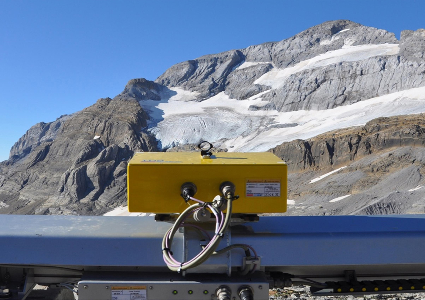
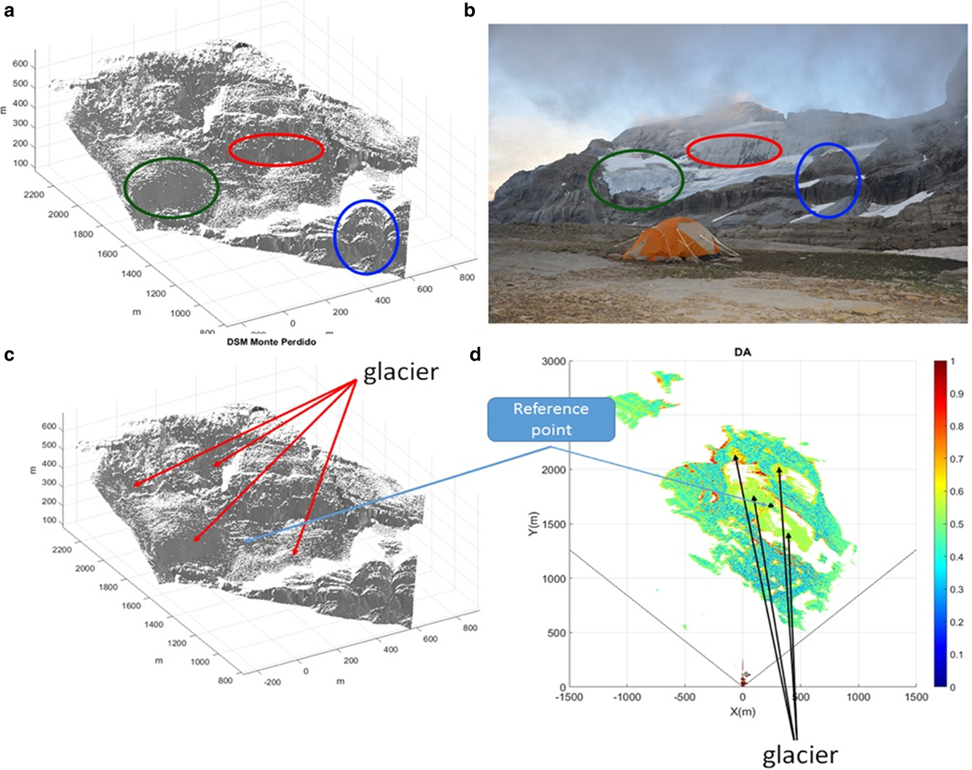
The GB-SAR was installed close to the TLS scan position (Fig. 1) which has a frontal view of the Monte Perdido Glacier. Figure 3 shows the point of view of the GB-SAR. The measurement campaign lasted 28 d, starting the 23 July 2015 and ending the 18 August 2015. The system used was the IBIS-L, produced by IDS spa. The power supply consisted of two solar panels of 140 Wps. The main system parameters are summarized in Table 2.
GB-SAR point of view.
Main GB-SAR acquisition parameters
Unfortunately, it was not possible to obtain continuous measurements during the whole campaign due to bad weather conditions affecting the efficiency of the solar panels, with periods of heavy rains and strong winds. The final dataset consisted of 163 images which were acquired in three different periods: 144 were acquired without interruption between 23 and 30 July. The system was then stopped because the wind destroyed one of the solar panels. The system was reactivated on 11 August and acquired 18 images over 2 d, and finally two images were acquired before removing the system on 18 August. To complete the analysis, the GB-SAR information was contextualized with meteorological data and with a Digital Surface Model (DSM) derived from the closest Terrestrial Laser Scanner campaign (September 2016). For this work, we only analysed the continuous data (from 23 to 30 July).
Figure 4 shows an interpretation of the GB-SAR image using a TLS DSM and identifying the different areas of the glacier in the radar image. The dispersion of amplitude shown in Figure 4d and coherence are parameters usually estimated in radar interferometry to identify the areas where the phase information used to retrieve the displacement of the monitored surface is statistically reliable according to Caduff and others (Reference Caduff, Schlunegger, Kos and Wiesmann2015); in this case, values lower than 0.6 can be considered trustworthy measurements.
(a and c) Digital elevation model generated from TLS data acquired from the same position of the GB-SAR. (b) Photo of the glacier from the GB-SAR point of view (summer 2016). The coloured ellipses in a and b identify the same areas in both images. (d) GB-SAR dispersion of amplitude (DA) image obtained from the whole dataset and represented in GB-SAR geometry.
Deriving deformation estimates from the GB-SAR interferometric phases is not a straightforward process. It requires complex processing in order to properly separate the different components that contribute to the phase differences: atmospheric effects, phase unwrapping and temporal decorrelation (see Monserrat and others, Reference Monserrat, Crosetto and Luzi2014). In most of the approaches described in the literature, the processing can be summarized in five steps: pixel selection, 2-D phase unwrapping, phase integration, estimation of the atmospheric component and displacement computation. A detailed description of the processing used for this work is provided by Dematteis and others (Reference Dematteis, Luzi, Giordan, Zucca and Allasia2017).
There were two different processing types: (1) processing only nocturnal data (i.e. 0000–0600) and (2) processing the entire dataset. The first was performed with the aim of minimizing the effects of the atmosphere, given that its behaviour is more stable during the night. The second was performed in order to fully exploit the whole dataset and to compare the velocity changes between day and night cycles. Before processing these datasets, an analysis of the images was performed in order to discard the noisier images (Dematteis and others, Reference Dematteis, Luzi, Giordan, Zucca and Allasia2017) resulting in 73 images discarded of 144. The final dataset consisted of 71 images.
3.3. Ground-penetrating radar
During the last decades, the techniques based on GPR have been widely used in cryospheric studies. Their use allows determination of thickness and characteristics of the underlying substrate. They also reveal the physical and structural properties of the different underground media: snowpack, ice or permafrost (Schwamborn and others, Reference Schwamborn, Heinzel and Schirrmeister2008; Arcone and Kreutz, Reference Arcone and Kreutz2009; Del Río and others, Reference Del Río, Rico, Serrano and Tejado2014; Liu and others, Reference Liu, Takahasi and Sato2014).
Ground-based GPR prospecting in Monte Perdido Glacier had serious difficulties due to the surface steepness (average slope 20° with wide areas exceeding 40°), frequent rockfalls and abundant water circulating on the surface and within the ice body (López-Moreno and others, Reference López-Moreno2016).
We conducted two GPR campaigns in 2016, in spring (30 April and 1 May), and in autumn (19–20 September). Figure 2 shows the prospecting itineraries followed during the field surveys, performed with a Måla Geoscience GPR system, using 50, 200 and 500 MHz antennas. The first campaign had little liquid water circulating above and in the glacier, and a smooth snow-covered surface, but the survey was carried out under adverse meteorological conditions (winds >60 km h−1 and temperatures less than −8°C). The existence of a thick snowpack required the discrimination between ice and snow to accurately quantify glacier thickness. In contrast, the autumn campaign was performed under optimal meteorological conditions but with abundant liquid water circulating over and within the ice body. The presence of water negatively affects GPR prospecting, partly because the water inclusions produce a lot of scattering (resulting in noisy radargrams) and partly because the attenuation of radar waves are highly sensitive to the presence of liquid water on ice (resulting in less intense radargrams) (Daniels, Reference Daniels1996; Murray and others, Reference Murray, Booth and Rippin2007; Bradford and others, Reference Bradford, Nichols, Mikesell and Harper2009).
In the first GPR campaign, we endeavoured to carry out a detailed multifrequency study of the glacier structure at the lower Monte Perdido Glacier. Due to the bad weather conditions and avalanche risk, we conducted only one profile, although using three different antennas of 50, 200 and 500 MHz, in order to determine the radio wave velocity (RWV) in the ice, the ice thickness and the glacier structure in the study area. During the autumn campaign, it was possible to perform much longer transects using 200 MHz antennas, covering wider areas of the glacier.
In the spring campaign, the 50 and 200 MHz antennas were respectively configured to reach a depth of 30–60 m, with resolutions of 0.9 and 0.25 m respectively (λ/4), estimated approximately a quarter of the wavelength of the GPR radio wave inside the ice. To properly characterize the snowpack, we also used a 500 MHz antenna, with a resolution of 0.09 m and a maximum depth capability of ~11 m. The autumn profiling covered as much glacier area as possible, prospecting ~2 km of profiles, walking on the glacier surface. The 200 MHz GPR was configured to reach maximum depths of up to 100 m, registering two traces per second, and using a DGPS Leica 1200 (postprocessed subsequently) for the trace positioning. However, the presence of water caused a very low signal to noise ratio, generating high uncertainty in the majority of the reflections, which led to ±5 m of uncertainty in estimations of ice thickness.
In order to determine ice thickness, we estimated the RWV in the underlying media assuming a simple model of two homogeneous and isotropic (in terms of velocity) layers (snow + ice), and using the diffraction hyperbolae method (e.g. Clarke and Bentley, Reference Clarke and Bentley1994; Moore and others, Reference Moore1999).
The model assumes that the underlying medium can be split into two different media with constant RWVs: (1) snow and (2) ice. The addition of two-way travel times (TWTT) through both media (T 1 and T 2, respectively) provides the total TWTT (T). This also can be applied for thicknesses measurement, relating thickness to TWTTs via RWVs (V 1, V 2 and V), thus obtaining the RWV in the second (deeper) layer and expressing it as:
 $$V_2 = \lpar {VT-V_1T_1} \rpar /\lpar {T-T_1} \rpar .$$
This method can generate large errors in the V 2 estimate (e.g. Benjumea and others, Reference Benjumea, Macheret, Navarro and Teixidó2003). The main sources of error are the use of hyperbolae from off-nadir diffractors (those that are out from the vertical profiling plane), and the unknown diffractor size. Both overestimate the RWV of the shallower layer, while underestimating the size of the reflector, although both effects diminish with depth.
4. RESULTS
4.1. Climatic context of the studied period
Figure 5 shows the interannual evolution of precipitation (accumulation period, December to April) and temperature (ablation period, May to September) at the Goriz station. Precipitation during the accumulation period shows strong interannual oscillations, ranging from 350 to 1360 mm, but it does not show any statistically significant temporal trend for the period 1982–2017. Mean temperature during ablation season also exhibits strong interannual variability and presents a statistically significant trend (Spearman's ρ: 0.42; a < 0.01) at a rate of 0.33°C decade−1. It is interesting to note that all values above the 75th percentile appear after 2003 and onwards.
Temporal series of (a) temperature (ablation season, May to September) and (b) mean precipitation (accumulation period, December to April) in Goriz station. The 2011–2016 period is highlighted with blue colour. Dashed lines indicate the mean and the 25th and 75th percentiles.
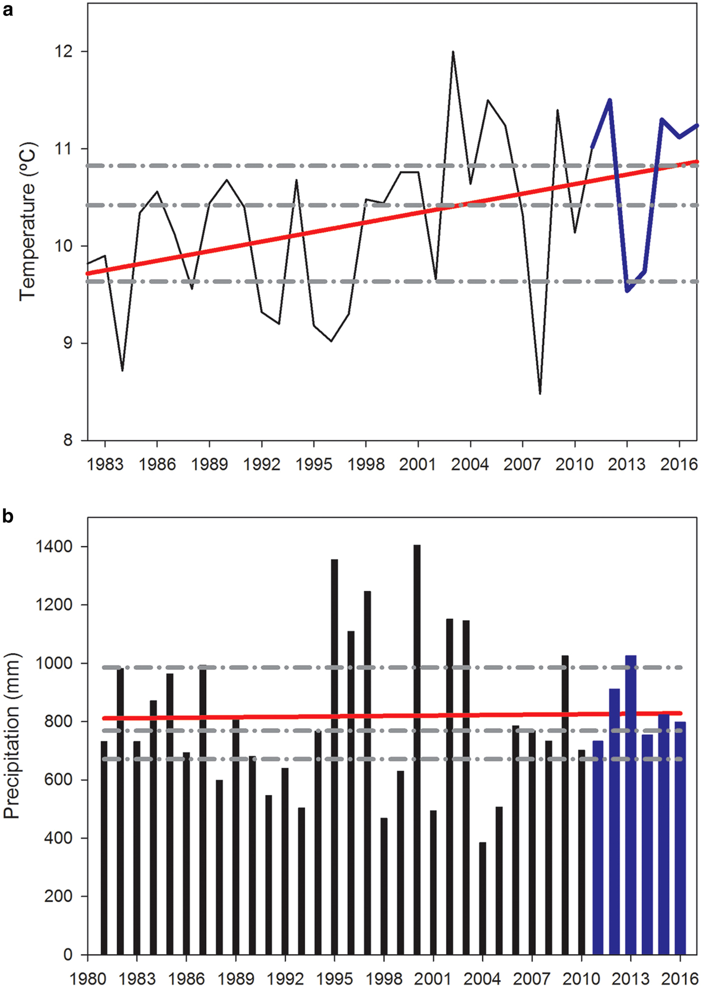
In line with the interannual variability of temperature and precipitation shown in Figure 5, the study period (2011–2017) exhibited very contrasting climatic conditions The period of 2011–12 was drier and warmer than the average; 2012–13 was drier than the long-term average with a very cool ablation period; 2013–14 was wet and cool; whereas the last 3 years exhibited average or above average precipitation and warm or very warm conditions during the ablation period.
4.2. Changes in elevation of ice surface and snow accumulation from terrestrial laser scanner
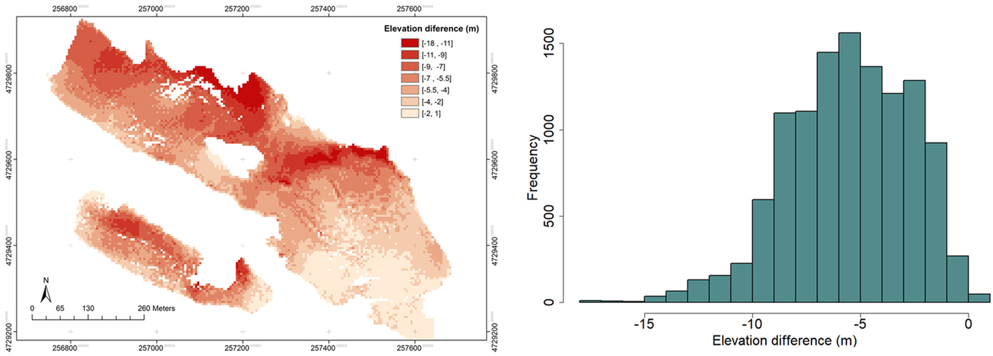
Figure 6 shows the difference in the elevation of the ice surface from September 2011 to September 2017 obtained through TLS. Table 3 shows the mean measured annual differences and the coefficient of correlation to illustrate the spatial consistence of changes in ice surface between the different analysed years. During the last 6 years, ice thickness of the glacier has reduced 6.1 m on average, but such losses have exhibited strong spatial and temporal differences. Thus, there are some sectors of the glacier where ice thickness decreased more than 15 m (mainly in the western sectors of the lower glacier and less elevated zones of the upper glacier) while other areas have exhibited almost no changes in ice elevation. The annual change in ice surface has exhibited very large interannual variability. Thus, during 2013–14 and 2015–16, the changes in the elevation of the ice surface were very small, being measured as very small average ice losses (−0.05 and −0.35 m, respectively), or being slightly dominated by accumulation (+0.35 m in 2012–13). The reductions in ice thickness were concentrated in 2011–12, 2014–15 and 2015–16, with average reductions of 1.8, 1.7 and 2.5 m, respectively. The coefficients of correlation show that the spatial pattern of ice thinning exhibits a statistical significant correlation (p < 0.01) during the 3 years of highest ice losses (2011–12, 2014–15 and 2016–17), but correlations were low with the spatial patterns observed in years with low changes in the elevation of the ice surface.
(a) Difference in the elevation of the ice surface from September 2011 to September 2017. (b) Frequency distribution of differences in elevation of ice surface from 2011 and 2017.
Changes in ice elevation measured with the TLS over the glacier from 2011 to 2017. The table also shows a correlation matrix of the different years from 100 points randomly selected over the glacier
*Indicates statistically significant correlations (p < 0.01).
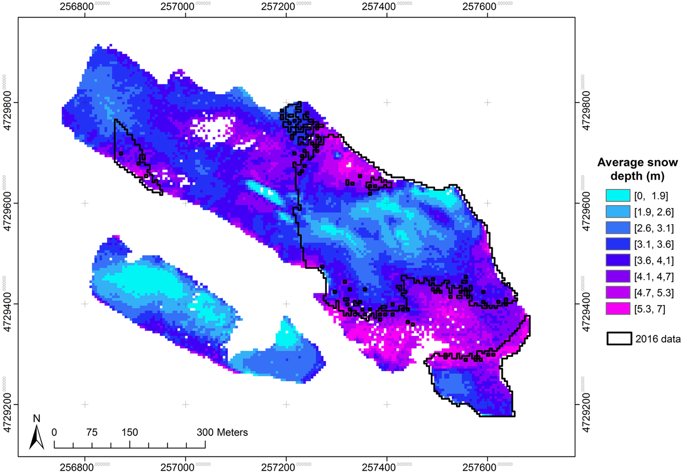
Figure 7 shows the average snow accumulation over the glacier in late spring of 2014, 2015 and 2017 (when no scanning limitations occurred and the whole glacier was scanned). Table 4 shows the mean accumulation over the glacier for the same years, and also for the area that was possible to be scanned in 2016. An average accumulation of 3.25 m (3.04 for the common area in the period 2014–2017) of snow (with an average snow density of 454 kg m−3) was registered for the 3 years. For the 2016 spring survey, the area from which it was possible to retrieve information with the TLS showed an average accumulation of 4.5 m, suggesting that it was the snowiest of the four analysed years. The data show that some areas, mainly located in the western part of the glaciers, registered average accumulations over 5 m, exceeding often 6–8 m; while some areas had very low average accumulation mainly due to wind and gravity redistribution. The interannual variability of average snow accumulation appears much lower than that observed for changes in the elevation of the ice surface. Only 2016 clearly registered a higher accumulation, with 33% more snow thickness compared with the average of the other 3 years. Measured snow density in the 4 years was rather constant, oscillating between 437 and 471 kg m−3. According to the correlation matrix, the spatial patterns of snow distribution were rather similar between 2014 and 2015 (r > 0.75, p < 0.01), but the distribution of 2016–17 exhibited more differences compared with 2014 and 2015 (r = 0.43 and 0.36; p > 0.01, respectively).
Average snow accumulation (m) for the years 2014, 2015 and 2017, and the area from which it was possible to retrieve snow depth data in 2016.
Snow accumulation measured with the TLS over the glacier during the 4 years. Values in parentheses correspond to the area where it was only possible to acquire data in 2016. The table also shows snow density measured in one snow pit over the glacier, and a correlation matrix for the years based on 100 points randomly selected over the glacier
*Indicates statistically significant correlations (p < 0.01).
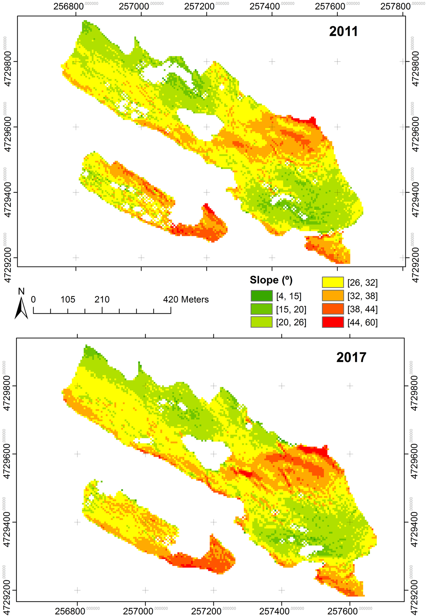
Figure 8 shows the slope angle of the glacier surface in 2011 and 2017. Despite being a relatively short period, the glacier surface exhibited significant changes, with a slight increase in average slope from 0.28° in 2011 to 0.31° in 2017. Some areas, mainly located at the bottom western part of the lower glacier, exhibited a decrease in slope angle as a consequence of the recent thinning of this frontal sector. Other wide areas have exhibited a clear increase in average slope, with a marked increase of the surface for slopes over 30°, which is a threshold often associated with noticeable reduction in snow accumulation (López-Moreno and others, Reference López-Moreno2017). Indeed, when Figures 7 and 8 are compared, it is possible to observe that areas with high slope angle are coincident with those with the lowest snow accumulation (r = −0.42; p < 0.01).
Slope angle of the glacier ice surface in 2011 and 2017.
4.3. Ice deformation and velocities from GB-SAR
Figure 9 shows the deformation velocity map obtained from the 71 images. The deformation values are in LOS, i.e. the measured displacements are a projection of the real displacement in the line between each point and the GB-SAR. Negative values represent points moving towards the GB-SAR. The values are between −4 cm d−1 (red) and 1 cm d−1 (blue). The estimated precision, based on the Std dev. of the accumulated displacement map, is 4.5 mm. It can be observed that most of the ice surface presents movement towards the GB-SAR, ranging from 1.5 to 4 cm d−1. However, it must be taken into account that sensitivity to the displacement changes has a high dependence on the main direction of movement. In this context, better sensitivity is obtained in the frontal part with respect to the GB-SAR (the green ellipse in Fig. 4b). The main reason for this is that the expected movements are almost parallel to the LOS. If we focus in this area, movements ranging from 2.5 to 3.5 cm d−1 are observed. However, other areas showed almost no movement during the analysed periods. These areas mainly correspond to the upper part of the easternmost ice body, and the majority of the western part of the glacier. A similar spatial pattern has been observed from the measured movement in seven ablation stakes, monitored by differential GPS each September for the period 2014–2017. Even the magnitudes measured in the ablation stakes (ranging from 32 cm a−1 to 9.98 m a−1) are slightly lower (note that ablation stakes are average daily values calculated from annual displacements) but comparable to those measured with GB-SAR.
Deformation velocity map in cm d−1 obtained from the whole GB-SAR dataset (71 images). Numbers indicate the time series depicted in Figure 10. Rectangles inform of the average daily displacement (cm a−1) measured in seven ablation stakes during 4 years (2014–2017) of observations (measured in September each year).
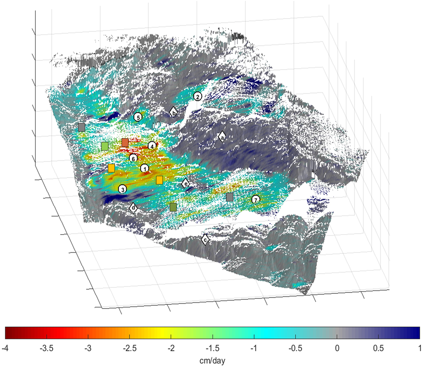
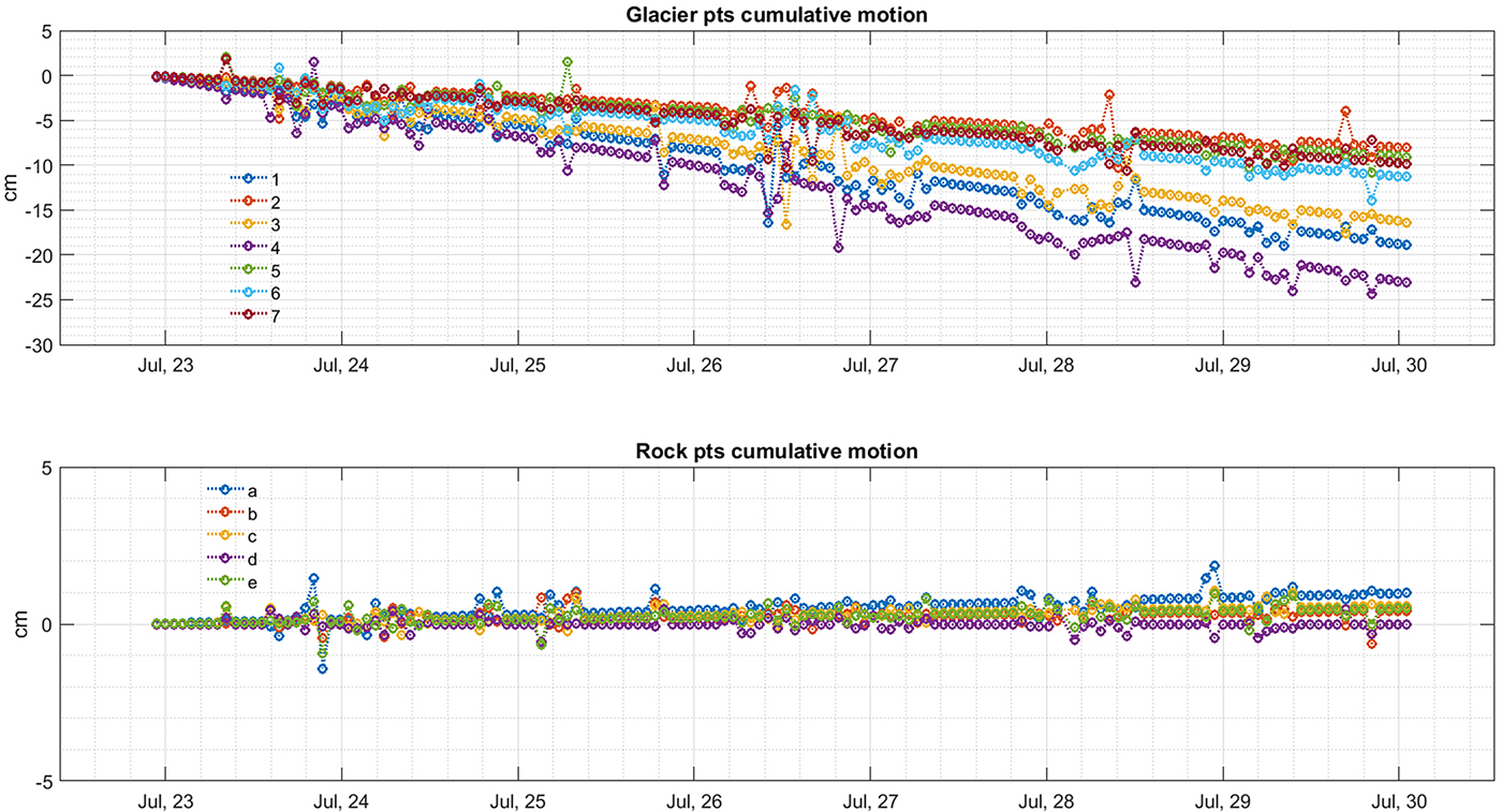
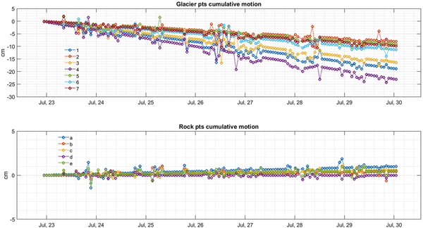
Figure 10 shows some examples of time series obtained for points 1–6 (depicted by circles) in Figure 9, and for the points (a–e, depicted as rhomboids) located in rock areas where no displacements are expected and observed: this check can be considered an estimate of the precision of the GB-SAR measurements (in order of mm); there are minor fluctuations and trend, which can be due to accumulation of atmospheric residue and noise introduced by ice melt runoff on the rock faces. Focusing on the moving points (1–7 in Fig. 9), the time series shows that the observed movements are almost linear. However, it is observed that during some nights the movement becomes slower, e.g. July 27 and 28. This has been confirmed by nocturnal images. These results show velocities ~50% slower during night time.
4.4. Ice thickness estimates and internal structure
Both the processing of the radar profiles and the RWV estimates have been implemented using the software ReflexW v7.6 (Sandmeier Geophysical Research, http://www.sandmeier-geo.de/reflexw.html). To estimate the RWV in the underlying media, we used the diffraction hyperbolae method in the spring profiles, assuming a simple model of two homogeneous and isotropic layers of snow (shallower layer 1) and ice (deeper layer 2). Since the autumn profiles did not contain diffraction hyperbolae of sufficient quality to apply this method, we used the spring results to estimate the RWV values for the whole study.
Figure 11 shows the three radargrams collected in the spring 2016 campaign, with a first post-processing consisting in energy decay correction, background removal and dewow. From the different hyperbolae in the radargrams collected with the 200 and 500 MHz antennas (T200 and T500 in Fig. 10), we estimate that V, the RWV for the averaged media, and V 1, the RWV for the snow, are 169 ± 4 and 200 ± 5 m μs−1, respectively. For these estimates, we assumed that the diffractor sizes were ~1 m (wavelength of the 200 MHz wave), large enough to generate strong hyperbolae at 200 MHz but small enough to explain the weaker hyperbolae at 50 MHz. Thus, knowing the RWVs and thicknesses of the mixed medium and of the snow layer, we use Eqn (1) to obtain the RWV in the ice layer, V 2 =163 ± 7 m μs−1. Then, we can estimate relative permittivities of 3.39 ± 0.30 and 2.25 ± 0.11 for ice and snow, respectively (Bogorodsky and others, Reference Bogorodsky, Bentley and Gudmandsen1985).
Radargrams obtained in spring (30 April/1 May) with 500 (T500), 200 (T200) and 50 (T50) MHz antennas.
Although this method is usually affected by large uncertainty, we consider that the resulting RWVs in this case are adequate, and we use them because the profiles contain a large amount of hyperbolae confirming such velocities, which diminishes the error. Using the estimated velocities, the maximum thickness we determined in the spring was 31.7 ± 1.3 m, located at a horizontal distance of 93 m from the start of the radargram. At that point, the thickness of the snow layer was 5.9 ± 0.3 m and the ice thickness was also at a maximum, reaching a value of 25.8 ± 1.6 m.
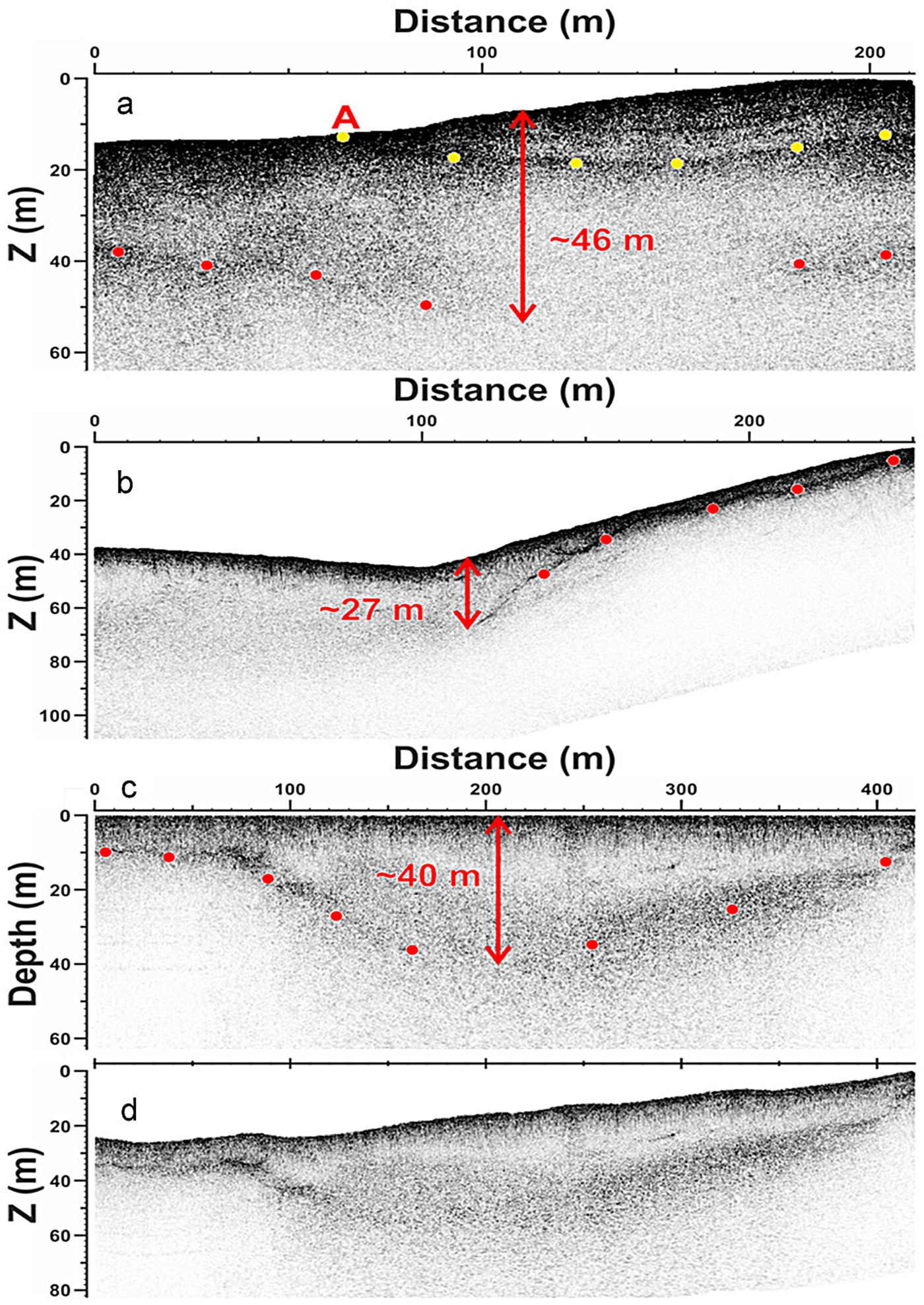
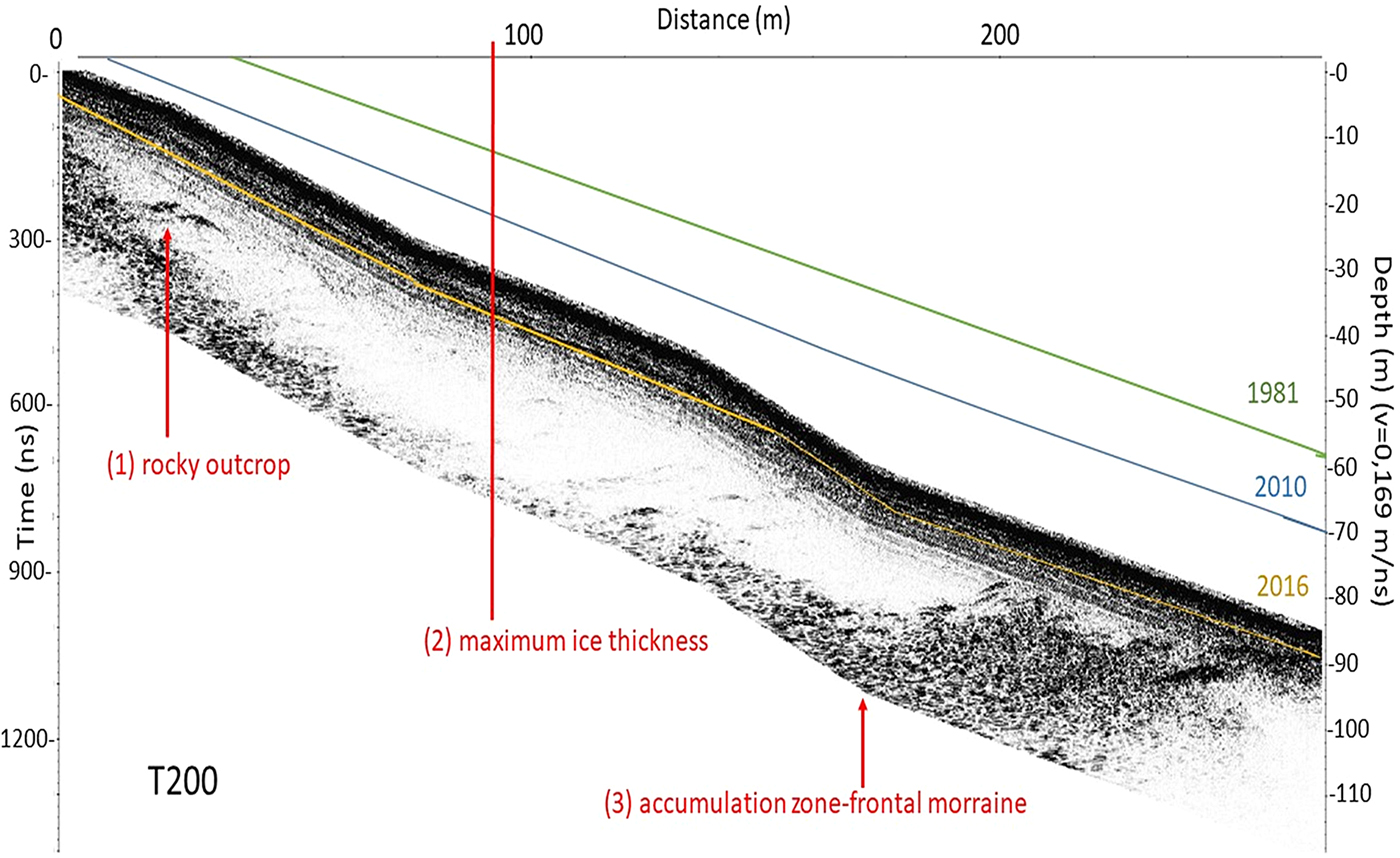
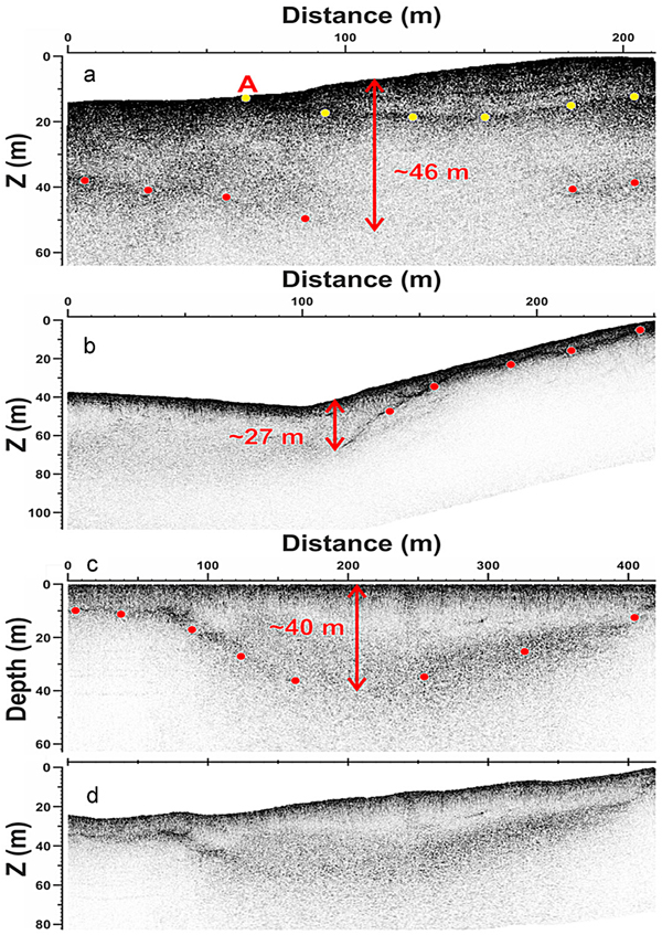
Figure 12 shows three examples of the 200 MHz radargrams conducted in the autumn. For their processing, we chose the RWV for the ice estimated from the spring profiles (i.e. 163 m μ−1). Their processing included horizontal and vertical filters, time-dependent signal amplification, dynamic correction, deconvolution, migration and time-to-depth conversion. Panels A, B and D also include topographic correction. Profile A, one of the set P1a in Figure 2, suggests the existence of more than 10 m of firn. The central part of the profile exhibits a very attenuated reflection of the basal bedrock, although a thickness of ~46 ± 5 m can be inferred. The first half of profile B (from the set P2a in Fig. 1) does not exhibit bedrock reflection, probably due to a thicker ice layer and the presence of circulating liquid water. However, a clear reflection starts at 27 ± 5 m depth. Profile C (from the set P3a in Fig. 2) is also shown in panel D after its topographic correction. It exhibits noticeable ice thickness in its central part (~40 ± 5 m), though with very diffuse reflection, probably due to the presence of abundant interstitial water and impurities near the bedrock. This radargram shows the existence of a marked concave shape in the bedrock (panel D), which could facilitate the accumulation of liquid water in this part of the glacier.
Examples of 200 MHz radargrams obtained in the autumn campaign. Red dots delineate the estimated basal zone, and yellow points indicate the estimated transition between ice and firn. Panels a, b and c show processed profiles, converted into depth and affected by a topographic correction, thus Z representing relative altitude from a datum placed at the highest point of the profile. Panels c and d represent the same profile, without and with such a topographic correction.
A more detailed picture of the glacier structure can be seen in Figure 13, which shows the T200 radargram of profile P1S, once processed (with additional gain filter, migration and topographic correction). It is possible to identify three vertical layers from top to bottom: (i) the snowpack composed of different layers; (ii) the next layer of firn; and the (iii) glacial ice. It suggests that boulders and tills compose the basal zone. In Figure 12 we have also shown the estimated evolution, since 1981, of the surface elevation at profile P1S, indicating the lowering of the glacier surface observed in the last decades.
Structure of the glacier obtained from the radargram 200 (T200) MHz after post-processing from GPR survey conducted in spring (P1S in Fig. 1). The estimated surface of the glacier from TLS data and previous geomatic analysis (López-Moreno and others, Reference López-Moreno2016) are also indicated.
5. DISCUSSION
Acquiring in situ observations of this glacier, although possible, was very challenging and very likely it will become more difficult due to increased steepness, ice collapses and rockfalls in the next years. The current characteristics of the glacier in terms of topography, existence of hollows and water circulating above and beneath the ice surface also made it difficult to properly apply GB-SAR and GPR methods. Also, the severe meteorological conditions are a limiting factor in the use of TLS in such a high mountain environment.
5.1. Interannual changes in thickness and slope of the Monte Perdido Glacier
Errors using TLS for calculating changes in the elevation of the ice surface were estimated at ±0.30 m at the working distance for this glacier (1000–2000 m from the scanning position; López-Moreno and others, Reference López-Moreno2016); and the error increased to ±0.40 m for the estimation of snow thickness, as a consequence. Slight instabilities of the tripod on frozen soils (Revuelto and others, Reference Revuelto2014) required point cloud alignment (ICP algorithm; Pomerleau and others, Reference Pomerleau, Colas and Siegwart2015) in the post-processing. In addition, unexpected windy conditions recorded in late April 2016 impeded proper scanning of the whole glacier, and it was only possible to cover an area of ~62% of the lower glacier. This shows the strong dependence on atmospheric conditions during TLS acquisition (Revuelto and others, Reference Revuelto2014).
Despite the uncertainties mentioned above, TLS has provided clear information on the irregular thinning of the ice body in time, occurring mostly in specific years and certain zones when average ice losses over the entire glacier exceed 1.5 m, whereas other years the glacier remained rather stable. To our knowledge, TLS has not been used yet for monitoring interannual snow accumulation on a glacier, although it has been used for isolated years with very similar uncertainty to that obtained in our studies (Xu and others, Reference Xu2017). Our observations have resulted in useful information on the dynamics of snow over the glacier at the end of the accumulation season. Snow has recorded less interannual variability than ice surface lowering, with variability lower than 30% with respect to the interannual average. The patterns of snow distribution tend to change from one year to another, with rather low correlation coefficients between years, probably due to wind redistribution effects under contrasting annual dominant directions (Dadic and others, Reference Dadic, Mott, Lehning and Burlando2010). However, for some years, high correlations have been observed, and thus longer observation periods may allow acquisition of stronger conclusions. In general, there is not a clear relationship between snow accumulation and the magnitude of ice losses during summer, since during years with high snow accumulation, the glacier has exhibited strong ice losses during the ablation period (i.e. 2016 and 2017). This could suggest that the annual mass balance of the glacier is dominated by melting during ablation rather than by accumulation during winter and spring. Additionally, some areas of the glacier have noticeably increased slope angle in the last 6 years, which may markedly affect snow accumulation in these areas. Indeed, these areas have presented bare ice at the end of the accumulation period, which could accelerate degradation of the glacier at these specific spots.
5.2. Estimation of ice deformation and glacier movement
The GB-SAR measurements have shown the potential of this technique to monitor glacier movements. The results have confirmed surficial movements during the monitored summer period ranging from 2.5 to 4 cm d−1 in LOS. Moreover, the results obtained using only nocturnal data have shown that the movement is, on average, up to 50% slower at night than during the day. We have also observed some variability in ice motion speed over different days. Values of ice motion speed from ablation stakes exhibited a very similar spatial pattern to that obtained from GB-SAR but, in general, lower speeds with maximum annual average displacements of 2.7 cm d−1, which could suggest a decrease in ice motion during the cold season, as it has been observed in other glaciers (Burgess and others, Reference Burgess, Larsen and Forster2013; Satyabala, Reference Satyabala2016). The results also showed one of the weakest points of the technique is dependence on the acquisition geometry. The main results have been obtained in the frontal part of the glacier with respect to GB-SAR point of view. In this area, sensitivity to displacement was high. However, in the more lateral area, sensitivity to displacement can be very small, preventing a direct interpretation of the results.
5.3. Ice thickness and internal structure
The application of GPR techniques was problematic in the autumn, probably due to the large amount of water circulating over and beneath the glacier surface. Nonetheless, it allowed us to estimate ice thickness (within an uncertainty of 5 m) for large areas of the glacier, revealing that it is still possible to find ice thicknesses between 30 and ~50 m in some sectors of the glacier. The GPR survey conducted in spring covered a much smaller area but provided noticeably better radargrams, with resolutions better than 1.5 m. The ice thickness measurements from both campaigns are compatible, thus confirming their results. However, the use of three different antennas in the spring profiling, and the clarity of their radargrams, allowed better identification of the internal structure of the snow cover and the ice, revealing that remnant ice has a high content of tills that may translate into a noticeable increase of debris cover as thawing continues.
The estimated values for the RWV, 200 and 163 m μs−1, and relative permittivities of 3.39 and 2.25 are consistent with those in snow and ice (Daniels, Reference Daniels1996; Eisen and others, Reference Eisen, Nixdorf, Wilhelms and Miller2002; Benjumea and others, Reference Benjumea, Macheret, Navarro and Teixidó2003).
5.4. Current behaviour of Monte Perdido Glacier and future expectations
Overall, results confirm the advanced stage of degradation of the Monte Perdido Glacier. At the beginning of this period, during 1981–2010, the thinning rate was measured by López-Moreno and others (Reference López-Moreno2016) at 0.6 ± 0.3 m a−1. However, the thinning of the glacier is accelerating, given that it has lost, on average, 6.1 m of ice thickness in the last 6 years (1 m a−1), with 10–15 m of ice loss in wide areas. Mean annual average ice depth loss reported in our study matches closely to the study of Marti and others (Reference Marti2015) for the Ossoue glacier, who reported a mean ice thinning between 20 and 50 m for the period 1983–2013. These values illustrate the critical situation of the glacier, considering that the ice thickness in most parts of the glacier is <30 m, and that the thicker ice measured is 46 ± 5 m. Assuming a similar trend in the future (e.g. not <1 m a−1), extinction of the entire glacier could be expected within the next 50 years. This dramatic situation is leading to further study the glacier ice in Monte Perdido from a paleoenvironmental point of view analysing an ice core retrieved in 2017 as a final opportunity to extract information of past climate conditions (e.g. determining the glacier stage during past warm periods such as the Medieval Climate Anomaly).
The hypothesis that glacier mass balance clearly responds to summer ablation more than winter and spring accumulation leads to a pessimistic scenario for the short-term future, since precipitation in the cold season has not shown clear trends in the past (Fig. 4) and projected scenarios do not inform of clear changes. However, spring and summer temperatures have significantly increased and are foreseen to continue increasing (López-Moreno and others, Reference López-Moreno2011), which means a longer and more intense ablation season. This situation is also evidenced by the very reduced, or inappreciable (with GB-SAR technique) movement in wide areas of the glacier, especially in the westernmost part of the glacier, where ice is near stagnant and ice losses are particularly high. The easternmost sector presents lower ice losses and areas with noticeable movement (annual average of 1.5–2.5 and 3–4.5 cm d−1 during summer 2015) and, in turn, it is also the area where a thicker ice has been measured. The glacier has not exhibited a slowdown yet in melt rates as could be hypothesized (DeBeer and Sharp, Reference Debeer and Sharp2009) for a very degraded ice body, and it could happen once most of the western part of the glacier disappears (which could occur two decades or less if current conditions persist). Only the eastern part of the glacier will last, and it is expected that it will melt at lower rates. The high content of till in the remnant ice, shown by GPR data, informs that debris cover, already rapidly increased in the last years, will expand and get thicker in coming years. Mass-balance measurements carried out in the Maladeta and Ossoue glaciers (together with Monte Perdido Glacier, the biggest glaciers in the Pyrenees) (Marti and others, Reference Marti2015) for the last years, and recent estimations of decline of glaciated surface for the entire Pyrenees (Rico and others, Reference Rico, Izaguirre, Serrano and López-Moreno2017), highlight that degradation of the Monte Perdido Glacier is highly representative of the current situation of the other 18 existing glaciers, which identifies the Pyrenean glaciers as some of the most endangered glaciers in the world.
6. CONCLUSIONS
Results shown in this study highlight the potential of combining information from TLS, GPR and GB-SAR to obtain valuable information on current conditions of the Monte Perdido Glacier and recent evolution. TLS data have allowed to determine an average ice thinning of 6.1 m for the period 2011–2017 (1 m a−1), with wide sectors exhibiting losses of 10–15 m of ice depth. There is not a clear relationship between snow accumulation and the magnitude of ice losses, suggesting that the annual mass balance would be dominated by melting during ablation season. GBSAR have allowed to quantify average ice motion of the glacier during summertime in 2.5–4.0 cm d−1. A fluctuation in ice speed is suggested by collected data during day and night period, and also a noticeable variability between different measurement days. GPR campaigns indicated that ice thickness in the glacier ranges among 30 and ~50 ± 5 m in the best preserved areas of the glacier. The maximum measured ice thickness for the glacier, the annual rates of ice thinning and the evidence of stagnation in much of the ice-covered area confirm the critical situation of the Monte Perdido glacier that could evolve to a glaciaret of very reduced size in the next three to five decades.
ACKNOWLEDGEMENTS
E. Alonso-González is supported by a FPI fellowship of the Spanish Ministry of Economy and Competitiveness (BES-2015-071466). J. Revuelto is supported by a Post-doctoral Fellowship of the AXA research foundation. This research was made possible partially by funding granted by the Junta de Extremadura and the Fondo Europeo de Desarrollo Regional-FEDER, through the reference GR15107 to the research group COMPHAS and the EXPLORA PaleoICE project (ref. CGL2015-72167-EXP), and CLIMPY (FEDER-POCTEFA). The research of J. Lapazaran and J. Otero was funded by the Spanish State Plan for Research and Development project CTM2014-56473-R. We thank the two anonymous reviewers and the scientific editor (Bernd Kulessa) for their constructive comments and help to improve our work.


 Open access