

Structural equation modeling (SEM; Jöreskog, Reference Jöreskog1969) enables modeling with latent and measured variables, and allows researchers to realize the power of causal modeling (Pearl, Reference Pearl2009). It has grown substantially in importance (Hershberger, Reference Hershberger2003). Despite its utility, learning, implementing and interpreting, these techniques have remained a bottleneck for many researchers, especially for more complex multiple-group models common in advanced fields such as behavior genetics. The advent of modular software such as OpenMx has provided tools for software solutions in this field (Boker et al., Reference Boker, Neale, Maes, Wilde, Spiegel, Brick and Fox2011; Neale et al., Reference Neale, Hunter, Pritikin, Zahery, Brick, Kirkpatrick and Boker2016). The present article describes umx, a package designed to give more immediate access, concise syntax and helpful defaults for path-based SEM, together with a set of high-level functions implementing matrix-based, multigroup twin modeling. Practical examples of umx usage are given. Users interested only in learning about twin modeling in umx may wish to skip to the section with that name.
Existing SEM Packages
while a number of closed-source commercial applications exist (e.g., Mplus; Muthén & Muthén, Reference Muthén and Muthén1998–2016), SAS proc calis (SAS Institute Inc., 2003), SPSS Amos (IBM Corp, 2013) and GLAMM in STATA (Stata Corp LP, 2016), there are now three open-source R packages for performing SEM: sem (Fox et al., Reference Fox, Nie and Byrnes2014); lavaan (Rosseel, Reference Rosseel2012); and OpenMx (Boker et al., Reference Boker, Neale, Maes, Wilde, Spiegel, Brick and Fox2011; Neale et al., Reference Neale, Hunter, Pritikin, Zahery, Brick, Kirkpatrick and Boker2016). As is common in R, these interoperate with an ecosystem of packages, such as semTools (semTools Contributors, 2016), Onyx (von Oertzen et al., Reference von Oertzen, Brandmaier and Tsang2015), ctsem, EasyMx, ifaTools, lvnet, metaSEM and semtree, to provide additional features.
sem includes functions for fitting general linear structural equation models, including both observed and latent variables, using the RAM (McArdle & Boker, Reference McArdle and Boker1990) approach. It also allows fitting structural equations in observed-variable models by two-stage least squares. Models are input using an ‘arrow specification’ with paths described in an intuitively straightforward notation encompassing regression coefficients (‘A -> B’), variances (‘A <-> A’) and covariances (‘A <-> B’). Models can be optimized against a maximum-likelihood objective assuming multivariate normality as well as multivariate-normal full-information maximum likelihood (FIML) in the presence of missing data, with alternative objectives including generalized least squares or user-specified objective functions. The sem package also implements multigroup models.
lavaan implements a similar string-based syntax for model description, comparable multigroup capability and a range of estimators including robust ML and variants of Weighted Least Squares (WLS). It outputs standard errors (SEs) including robust and bootstrap SEs, along with standard fit indices and statistics such as Satorra-Bentler, Satterthwaite and Bollen-Stine bootstrap. lavaan can handle missing data via FIML estimation. It allows the use of linear and nonlinear equality (and inequality) constraints via a string syntax; for example, to equate model parameters ‘a1’ and ‘a2’, the user includes the following in their model statement: ‘a1 = a2’. More complex statements are supported; for instance, ‘a1 + a2 + a3 = 3’. As of version 0.5, lavaan supports models with mixtures of binary, ordinal and continuous observed variables. Exogenous categorical variables are supported via dummy variables, with additional variables being created to represent the levels of nominal measures with more than two levels. Modeling of binary and ordinal endogenous categorical variables (but not nominal) is supported by a three-stage WLS approach. lavaan outputs results in a format familiar to users of Mplus and EQS. It is also possible to translate Mplus code into lavaan format via the function mplus2lavaan.
OpenMx provides a sophisticated kit of basic objects for building structural equation models, including modeling via arbitrary matrices, algebras, constraints and fit-functions. It also supports RAM (McArdle & Boker, Reference McArdle and Boker1990) and LISREL (Jöreskog, Reference Jöreskog1969) path-based models. It accepts both summary and raw data and arbitrary mixtures of continuous, ordinal and binary data. FIML analysis with missing data is supported, as is WLS. With raw data, models may include row-specific values (definition variables). Multiple-group models are supported, and constraints and equalities may be implemented via label-based equating and algebra-based linear and nonlinear constraint specification. The OpenMx package includes two open-source optimization packages — CSOLNP and SLSQP — and can use the closed-source NPSOL optimizer. OpenMx has developed a strong following among geneticists and twin researchers, reflected in several hundred citations in published projects, many of which rely on testing complex models, often with constraints, using data comprising mixtures of binary, ordinal and continuous data, with missingness, and wide-format data comprising multiple genetically related groups (in particular, identical and fraternal twins, siblings, parents, grand-parents, offspring and adoptive parents), with data nested in these family structures.
Accessible Modeling with Concise Syntax and Helpful Defaults
The umx package evolved over the last 7 years in response to modeling demands experienced in practical path-based modeling and matrix-based behavior genetics structural modeling and in teaching SEM. Its concise syntax aids in time-constrained lessons and affords researchers the ability to rapidly implement and modify new models, while high-level implementations of complex models increase the speed and reliability of behavior genetics modeling. Attention was paid to smart defaults — for instance, setting start values and automatically labeling paths — as well as ensuring functions handle a wide range of inputs, so that users can offer up a wide range of data and get the results they expect. For instance, models can accept not only continuous data, but mixtures of ordinal and continuous data, with the umx functions handling the error-prone process of setting up threshold matrices and integrating these with latent variables. To aid learning and help users correct coding mistakes, help files contain substantial, well-commented practical code examples oriented toward being used directly in class instruction or self-directed learning. umx functions include significant error checking. Errors and warnings are written to explain both why a problem occurred and how to fix it. Where possible, what was expected as input and what the user offered up are succinctly summarized. In addition, example code likely to fix the problem is included in the warning.
Finally, umx provides methods for generating graphical and tabular output suitable for publication (e.g., Table 2). Function names and parameters have been refined based on feedback and a drive for consistency and memorability. Where appropriate, these are implemented as S3 methods well known to R users: for instance, plot() and residuals(). A number of papers using the package have been published (Archontaki et al., Reference Archontaki, Lewis and Bates2013; Ritchie & Bates, Reference Ritchie and Bates2013) and umx is under active development — with updates on CRAN every month or two, and a road-map of future extensions of the twin modeling functions including use of WLS objectives, 5-group twin models, direct variance (rather than Cholesky) based models, bivariate G × E models, simplex models, as well as multivariate sex-limitation models using correlated factors rather than Cholesky factorization approach (Maes et al., Reference Maes, Sullivan, Bulik, Neale, Prescott, Eaves and Kendler2004).
In total, the package includes approximately 140 high- and low-level helpers for such tasks as data processing, creating and editing data structures, updating model parameters and reporting. The functions provided by umx may be grouped under three headings:
1. Model building and reporting functions.
2. Functions implementing behavior genetic models.
3. Wrappers and helpers to simplify or enhance model building and data wrangling.
In the next section, umx’s path-based functions are introduced in the context of practical models, such as that shown in Figure 1. The second major section covers behavior genetic modeling in umx. Not detailed here, we briefly note some of the additional helper functions available in umx. While the numerous wrapper and helper functions make little claim to innovation, they offer increased speed of coding, reduced errors and more readable code. For instance, umxMatrix is a wrapper for mxMatrix that places the matrix name as the first parameter (increasing readability) and automatically adds labels in a standard format. Other helpers simplify repetitive tasks, such as generating lists of twin variables from base names, and residualizing family-based data.
Example CFA path diagram, showing standardized path estimates.

Installing the Package
umx can be installed using the standard R-code to access the CRAN version of the package.
The library is loaded as usual with
This document assumes umx version 1.8.0 or higher. The current package version can be shown with:
This gives a compact summary integrating information available via sessionInfo(), but also showing the optimizer used and other information.
Current developer betas are available on www.github.com. These may have new features or respond to user requests between CRAN releases. They are installed using:
umx also aids installing custom versions of OpenMx via the install. OpenMx() function. These include versions with proprietary optimizers or nightly builds.
Path-Based Models in umx
Path-Based Models Using umxRAM and umxPath
In umx, a path-based structural model consists of a model container, some data and a collection of paths. The model container is the umxRAM function. This specifies the data, a name for the model, options such as autoRun, and, importantly, a collection of umxPaths specifying the paths that make up the model. As coding is often best learned by doing, we introduce these functions via building the Confirmatory Factor Analysis (CFA) model shown in Figure 1. To build this CFA model, we will specify three things:
1. An arbitrary name — ‘CFA’
2. The data (in this case a built-in dataset demoOneFactor containing five correlated variables x1:x5). In keeping with familiar R functions such as ‘lm’, the data to be modeled are provided via the data parameter. The umxRAM function can accept a data frame, covariance matrix or mxData as data.
3. The paths of which the model is composed. The paths required in this model are those needed to create a latent variable ‘G’ with mean of 0 and variance of 1, the five manifest variables x1:x5, each with freely estimated mean and variance, and single-headed paths from G to each of the five manifest variables.
Building, running and saving this model in its run state for possible modification or comparison, along with producing summary data and a plot, can be done in a few lines (excluding comments, loading the library and data) of model code shown below as ‘CFA Code’. This five-line example might be two lines in lavaan, highlighting the choice in umx to assume fewer defaults.
CFA Code
This code block builds the model, echoing to the console which latent and manifest variables were created. By default, umxRAM also runs the model, plots it graphically and prints a brief fit statistic summary:
 $$\chi 2\left( 5 \right) = 7.4, \,p = .193;\,{\rm{ CFI }} = 0.999;\,{\rm{ TLI }} = 0.999;\,{\rm{ RMSEA }} = 0.031$$
Two aspects of this code are noteworthy. First, we did not explicitly specify a list of manifest and latent variables contained in the model. Instead, umxRAM maps these from the data provided. Any variable name not found in the data is assumed to be a latent variable. As with lm, unused variables are excluded from the model automatically. Second, we did not need to specify starting values for the parameters. umx generates feasible start values. Currently, manifest variable means are set to the observed means, residual variances are set to 80% of the observed variance of each variable and single-headed paths are set to a positive starting value. The start-value strategy is subject to improvement and will be documented in the help for umxRAM.
umxPath in Detail
umxPath creates paths in a model using a compact syntax, describing a full range of path types and settings. A complete list of umxPath keywords is set out in Table 1.
Table of umxPath options
For example, to create a two-headed path allowing a variable ‘a’ to covary with variable ‘b’, with the covariance fixed at the value 1, the user would add a call to
To specify a mean for a manifest or latent variable, say the variable ‘b’, the umxPath code would be umxPath(means = “b”). As specifying the mean and variance of variables is such a common task, umxPath supports doing both in one line with the v1m0 and v.m. parameters we saw used in the above CFA model to specify normalized (fixed mean = 0, variance = 1) or freely estimated variables, respectively.
Parameter Labels
The umx package automatically adds labels to all parameters of a model. These labels allow the user not only to get and set the values of parameters by label, but also to equate parameters by setting their labels to be the same (see section on umxModify below).
One-headed paths are labeled ‘Var1_to_Var2’. Thus the path umxPath(“IQ”, to = “earnings”) would be labeled ‘IQ_to_earnings’. For two-headed paths, ‘_to_’ is replaced with ‘_with_’. This is consistent with Onyx (von Oertzen et al., Reference von Oertzen, Brandmaier and Tsang2015). Future versions of umx may extend the labeling scheme to encode more information in each label, for instance, the extra information captured in LISREL-type models.
For matrix-style models (such as the behavior genetic twin models described below), umx uses a more general labeling scheme, in which labels are a concatenation of the matrix name, an underscore, the letter ‘r’ for row, the row number, followed by the letter ‘c’ for ‘column’ and, finally, the column number of the matrix cell. The following code returns the $labels slot of a matrix ‘means’ to show an example of this labeling scheme:
Controlling Graphical and Summary Output
A parameter table (see Table 2) can be requested from umxRAM by setting the showEstimates parameter to ‘std’. More control and creation of summary output tables and plots is possible, however, using umxSummary on the model returned from umxRAM.
Example output table from umxSummary
umxSummary
Output from umxSummary can be as little as a line of fit information (the default) or a table of standardized or raw estimates (requested with show = “std” or show = “raw”). Example output from umxSummary(cfa1, show = “std”) is shown in Table 2.
This report is customizable, with parameters to filter non-significant (‘NS’) or significant (‘SIG’) parameters and to show or hide SE and RMSEA_CI columns. The summary table can also be directed to different outputs. By default, the table is composed in markdown, and this is written to the console. Alternative formats are possible, for instance, LATEX. Table format can be set using umx_set_table_format. Markdown is easy to read in the console or to include in a reproducible document. If the format is html, a file is opened in the user’s browser. This is useful for copying the formatted table into a word processor.
Plot
umx includes S3 plot methods for RAM and twin models. These rely on the dot language, invented at Bell Laboratories (as was S: the ancestor of R) to specify graphs in a text-based format of edges and vertices, analogous to the way that the LATEX system separates content from layout. Plots from umx are displayed in the user’s browser courtesy of the DiagrammR package.
The defaults for diagrams encourage users to produce mathematically complete diagrams. This is important for communication and scientific replication, and so we encourage it. By default, in addition to free paths, plot displays paths fixed at non-zero values (e.g. the unit variance of ‘G’ in Figure 1). This can be changed using the ‘fixed=‘ option. Similarly, by default, plot draws the means model (paths from the ‘one’ triangle). This can be toggled using the ‘means=’ parameter. plot can also standardize the model using ‘std = TRUE’, and control numeric precision (with the digits parameter). Other options include control over how residuals are drawn. By default, these appear as conventional circles with double-headed arrows.
Plotting is useful not only to display final models, but also may be used during model construction to verify or test what the code build to date is specifying. To make this easier when the user is “sketching out” ideas, requiring the data implied by the model paths, the user can simply offer up a list of variable names expected to be encountered as manifests and write the model they wish to visualize. For instance, to explore the unique.pairs construction of umxPath, the following model could be plotted:
For publication purposes, further processing of the diagram is often desirable. This is done by editing the file created by plot. The graph is written to a text file, by default ‘model_name.gv’. This can be overridden by setting the file = parameter to the desired file name. This file can be edited using either open-source graph visualization software available at http://www.graphviz.org, or closed software such as Omnigraffle®, or Visio®.
Inspecting Model Parameters and Residuals
Often, we wish to see a subset of estimates in a model. As shown above, umxSummary can filter the output according to whether parameters are significant or not, that is, umxSummary(cfa1, show=“std”, filter = “SIG”). The generic coef function can return a list of model coefficients. umx provides the convenience function parameters, which adds support for filtering by name and value and returns the parameters and estimates of a model as a neatly formatted table; for example, this snippet will show the parameters of model cfa1 estimated as greater than 0.5, and whose label contains the string ‘x2’:
Another common need in modeling is to inspect the residuals, that is, the observed — expected statistics. umx implements a residual method. Table 3 shows these for the cfa1 model. The user can zoom in on specific values with the suppress parameter. For instance, this call will hide residuals <.005:
Result of the residuals function on model ‘cfa1’
Modifying and Comparing Models
Model comparison and modification is a key modeling task (MacCallum, Reference MacCallum2003). Here, we introduce the umx functions enabling these tasks in the context of a classic example, modified from Duncan et al. (Reference Duncan, Haller and Portes1968); (see Figure 2). This is a moderately complex model, often used in teaching because of the range of structural model elements it displays.
A model of aspiration (modified from Duncan et al., Reference Duncan, Haller and Portes1968).
The code this model is shown in Code block 1 (see next page). This model introduces some new features and reinforces others already discussed. It is presented in three parts. First, reading in data. This uses a helper function included in umx for converting lower matrices to symmetrical, full matrices. There are many helpers such as this included in umx, and readers who adopt the package in their work will find these documented in the help for the package, where they are conveniently grouped in functional families:
Next, we make some useful lists of variables to use when creating paths. These will help reduce errors and increase the readability of code:
Finally, we build the model using the data and variable lists created above:
Modifying Models
The model fits well, χ2(22) = 24.59, p = .317; CFI = 0.997; TLI = 0.993; RMSEA = 0.02. However, for theoretically interesting models, the user will typically wish to test different versions of the model, dropping or adding paths corresponding to alternative hypotheses. The umxModify function supports this task, updating the model, giving the model a new name, running the new model and printing a table comparing fits of the old and new models.
In its simplest use, paths to be dropped are passed in as a vector or labels to the update parameter. The following code snippet will run a modified version of our example CFA, with the paths ‘RespLatentAsp to FrndLatentAsp’ and ‘FrndLatentAsp to RespLatentAsp’ dropped (fixed at zero). The new model is renamed to reflect this, and fit-comparison table printed (See Table 4):
Comparison of effect of dropping reciprocal influence from the duncan model
By default, updated paths are fixed at zero, but any value is possible via the values argument. Regular expressions can be used to pick out parameters that match a given pattern. A regular expression is a search pattern with powerful features greatly exceeding normal wildcards. While regular expressions are somewhat complex to learn, they repay the user in a wide range of computing applications and allow more compact syntax.
As an instance of using regular expressions in updating a model, consider a user who wants to test the effect of dropping all paths from ‘G’ in the cfa1 model. By label, these all begin with the string ‘G_to_’, followed by a variable name; for example, ‘G_to_x1’. Rather than listing each label in the update parameter, a regular expression that matches all instances could be used. Something as simple as ‘G_to_.*’ would work in this case (i.e., any character (‘.’) repeated any number of times ‘*’, matching any characters following “G_to_”). For more explicit safety, the regular expression anchor character (‘^’) could be used to ensure the match starts at the first character of the label, whereas ‘G_to_.*’ would match labels such as ‘notG_to_x1’, the carat (‘^’) prevents this by anchoring the expression at the first character. An example in R code would be:
umxModify can also be used to add or replace objects in models, for instance, if a umxPath is passed in to the ‘update’ parameter, the path will be added to the model.
Equating Model Parameters
In addition to modifying a model by dropping or adding parameters, a second common task in modeling is to equate parameters — setting two or more paths to have the same value. These parameters are picked out via their labels and setting two or more parameters to have the same value is accomplished by setting one set of parameters to have the same label(s) as a master set of parameters, thus constraining them to take the same value during model fitting.
This can be done using umxModify, which is useful for one-step modifications. This is done using the master parameter to set a master label or labels, for example, master = ‘G_toX1’, and update to set the additional label(s) which are to be equated (take the same value as) the master label. Because the process of equating parameters often occurs when building models (rather than modifying an already-run model), umx provides a dedicated function, umxEquate, which is useful when model building as by default, it does not run the new model.
As an example of using umxEquate, based on the duncan1 model, we might test if the effect of IQ on aspiration levels can be equated for respondent and friend. This is done by making a new model in which they are equated and comparing the two models as follows (Table 5):
Comparison of equating IQ effects in respondents and friends
Comparing Models
The table of model comparison output from umxModify is shown in Table 4. This comparison table can be generated directly using the umxCompare function. umxCompare takes one or more base models and one or more comparison models and prints a table of model comparisons. This includes a column directing the reader to the base model used for each comparison. The table is formatted with control over precision via the standard digits parameter. It can report the results to the console, or else open a browser table for pasting into a word processor. Printing to console is by default in markdown style (change this with umx_set_table_format set to one of latex, html, markdown, pandoc or rst). If report = “inline” is selected, umxCompare also reports the output in one or more sentences to help the user describe the results in text form. An example of using this function is given below: it will print a plain English description (the new model name is used to describe what was done and will need some editing). An example of this format is:
The output from the above code snippet is ‘The hypothesis that no reciprocal influence was tested by dropping no reciprocal influence from Duncan. This caused a significant loss of fit, χ2(2) = 19.51, p ≤ .001: AIC = −3.902’.
To open the output as an html table in a browser, say:
There are numerous additional functions in the umx library facilitating model interrogation; some are discussed at the end of this paper. For a complete listing, however, we direct the reader to the package help “?umx” and to the tutorial site for umx: http://tbates.github.io Next, we turn to twin modeling.
Behavior Genetic Twin Modeling
A major goal of umx was to provide support for common twin models, including Cholesky, Common-Pathway (CP), Independent-Pathway (IP) and gene × environment moderation models, with full support for tables and graphical output suitable for publication, as well as support for model comparison and modification. These functions are outlined below, beginning with a brief introduction to a common twin model (see Figure 3).
Genetic (A) components of a tri-variate ACE model (C and E not shown) in graphical (left panel) and matrix (right panel) forms.
Twin Models and Matrix-Based Modeling
Twin and family modeling takes advantage of classes of genetic and environmental covariance present in nature. For example, ‘identical’ or monozygotic (MZ) twins who share 100% of their genes, and fraternal (DZ: dizygotic) twins who share, on average, half of their genes, siblings, who also share 50% of their genes, but differ in year of birth, adoptees who are unrelated genetically to their rearing family, but who share that family environment. These classes of relatedness allow researchers to specify proposed structural and measurement models of their phenotype(s) of interest and to model many types of relatedness using multiple-group models that are fitted simultaneously to arrive at estimates of genetic and environmental variance consistent with the covariances found among the variables in the different groups of relatedness (Knopik et al., Reference Knopik, Neiderhiser, DeFries and Plomin2016; Neale & Maes, Reference Neale and Maes1996; Yong-Kyu, Reference Yong-Kyu2009). A classic approach to modeling data such as these is shown in Figure 3. This shows the decomposition of variance in behavior ‘x’ measured in two related individuals — either MZ twins or DZ twins — into additive genetic (A), shared environmental (C) and unique environmental (E) components. There are two groups in the model, one for each of the data sets. The correlation between A1 and A2 is fixed at 1 (all variable genes shared) in the MZ group, and at .5 for the DZ group (reflecting their 50% sharing of variable genes). umx implements this ACE model as a function — umxACE — and it is described in more detail below.
The ACE model decomposes phenotypic variance into additive genetic (A), unique environ- mental (E), and one of either shared environment (C) or non-additive genetic effects (D). This latter restriction emerges due to confounding of C and D when data are available from only MZ and DZ twin pairs reared together. The Cholesky or lower-triangle decomposition allows a model that is both sure to be solvable and it provides a saturated model against which models with fewer parameters can be compared. This model creates as many latent A, C and E variables as there are phenotypes, and, moving from left to right, decomposes the variance in each component into successively restricted factors (see Figure 4).
Cholesky decomposition (ACE model) of variance in behavior (x) in twin-1 and twin-2, decomposed into A (additive genetic), C (Shared environmental) and E (unique environmental) components. There are two groups in the model: Identical (MZ) twins and Fraternal (DZ) twins.
For efficiency, twin models in umx are implemented using a matrix-based approach (rather than the path approach used in Section 2). Each of the A, C and E components are modeled using square matrices, with the same number of rows and columns as there are variables under analysis. These in turn are formed from the product of lower-triangle matrices a, c and e respectively, multiplied by their transpose to form the variance component matrices (e.g., A = aa′). The utility of the Cholesky factorization is the product of a lower-triangular matrix and its transpose; for example, aa′ is guaranteed to be positive definite. The total phenotypic (observed) covariance is modeled as the sum of these three components: Vp = A + C + E.
Figure 4 shows how the path diagram is mapped onto matrices in the case of the additive genetic (A) matrix. As shown, the latent additive genetic variables form the columns of the A matrix. The variables are mapped to rows of this matrix, and paths from a latent variable to a manifest variable appear in the appropriate cell, for instance, the value of the path from A2 to var2 appears in cell A[2, 2] of matrix A.
The ACE Cholesky Model
The multivariate ACE or Cholesky model (Neale & Maes, Reference Neale and Maes1996) is implemented in the function umxACE (see Figure 4). This function can be used to fit an ACE model to a single variable to decompose its variance as shown in the example below. It can also be applied to two (bivariate) or more (multivariate) models, decomposing not only the variance, but also the covariance of the traits. We should note here that some of the text and images in this and other sections are used also in the package documentation of umx. This flow has been in both directions, with text written for this paper, and improved by helpful comments from reviewers and the editors flowing into umx documentation updates.
The umxACE function accepts either raw or summary (covariance) data, offering up suitable covariance matrices to mzData and dzData and entering the number of subjects in each via numObsDZ and numObsMZ. In an important capability, the model transparently handles ordinal (binary or multi-level ordered factor data) inputs and can handle mixtures of continuous, binary and ordinal data in any combination. This involves setting up threshold matrices for binary and ordinal data, which are modeled as thresholds applied to underlying latent variables.
It is often desirable to include covariates within twin models. We currently support ACE models with fixed covariates (covariates included in the means model) for continuous variables, and as random effects (i.e., modeled in the covariance matrix, allowed to covary with the main variables of interest (Neale & Martin, Reference Neale and Martin1989). In the next major version of umx, this functionality will be enhanced to allow modeling covariates in ordinal and mixed data across all twin models.
Weighting of individual data rows is supported in umxACE. In this case, the model is estimated for each row individually, the likelihood of each row is multiplied by its weight and the logarithm is taken. These weighted log-likelihoods are then summed to form the model log- likelihood, which is to be maximized (by minimizing the -2ln(Likelihood)). In addition, umxACE supports varying the DZ genetic association (defaulting to .5) to allow exploring assortative mating effects, as well as varying the DZ ‘C’ factor from 1 (the default for modeling family-level effects shared 100% by twins in a pair), to .25 to model dominance effects. This weighting feature is used in Section Window-based G × E section.
When it comes to interpretation and graphing, models built by umxACE can be plotted and summarized using plot and umxSummary methods. umxSummary can report summary A, C and E multivariate path coefficients, along with model fit indices and genetic correlations. The umx package provides custom plot methods to handle graphical reporting of twin models, including ACE models, and other models discussed below. This provides output as seen in Figure 4.
ACE Examples
We first set up data for a summary-data ACE analysis of weight data (using a built-in example data set from the Australian twin sample of Professor Nick Martin (Martin & Jardine, Reference Martin, Jardine, Modgil and Modgil1986; Martin et al., Reference Martin, Eaves, Heath, Jardine, Feingold and Eysenck1986):
The next code block uses umxACE to build and run the model.
umxACE prints feedback to the console, noting that the variables are continuous and that the data have been treated as raw. It then prints the fit
 $$ - 2 \times {\rm {log(Likelihood)}} = 12186.28({\rm{df}} = 4)$$
and outputs a plot of the fitted model (see Figure 5) and a table of the fitted parameters (Table 6). By default, the report table is written to the console in the format set by umx_set_table_format.
Output from plot(m1) for univariate ACE model of weight, rendered as default in DiagrammR (left) and after editing in Omnigraffle (right graphic).
Standardized path loadings for ACE model
The tabular output can also be requested at any time with umxSummary. Among other options, the user can request the genetic and environmental correlations with showRg = TRUE. If confidence intervals have been computed, these can be displayed with CIs = TRUE. The user can control output precision using the digits parameter. The following snippet creates a tabular summary of the unstandardized model (note, by default it will also plot the model. This can be controlled with umx_set_auto_plot(FALSE)). The function help (?umxACE) gives extensive examples, including for binary, ordinal and joint-ordinal cases:
Using Labels to Drop Paths in Twin Models
We noted above how labels can be used to update a model. For twin models, such model reduction by dropping paths is routine. For instance, to examine the effects of shared or family-level environment, we may wish to update this model by dropping the C (shared environment) paths. The matrix-based model labeling scheme (used in all the twin models) follows a systematic pattern, with the path coefficients underlying the A, C and E factors stored in matrices named a, c and e. We can view the c parameters with a call to parameters:
This reveals the following 4-parameter labels (and their current (unstandardized) estimated values) (See Table 7). It shows the four matrices for free parameters — a, c, e and expMean — each with 1 row and 1 column as this is a univariate model.
Free paths loadings for ACE model
These labels take the form: matrix name, ‘_r’ followed by a row number, then ‘c’ followed by the column number of the matrix cell containing the parameter; for example, matrix a row 1 column 2 would be labeled ‘a_r1c2’.
A straightforward way to drop the shared environment paths we wish to test is using the update option of umxModify. For example, this code snippet will test the effect of dropping the first latent C trait on the second variable in the model:
As shown in the resulting table of fit comparison table (Table 8), this parameter could be dropped without significant loss of fit. We next discuss a nested model, the CP model.
Fit comparison of full ACE model and AE model
CP Model
The CP model provides a powerful tool for theory-based decomposition of genetic and environmental differences (Neale & Maes, Reference Neale and Maes1996). This allows one to test, for instance, if genes and environment work through a common latent personality trait (Lewis & Bates, Reference Lewis and Bates2014), or to test claims regarding the specificity or generality of a theorized latent psychological or other construct (Lewis & Bates, Reference Lewis and Bates2010). umxCP supports CP modeling for pairs of MZ and DZ twins reared together to model the genetic and environmental structure of multiple phenotypes according to one or more CPs. As can be seen at the bottom of Figure 6, each phenotype also has A, C and E influences specific to that phenotype.
CP twin model with three common factors (CF1, CF2 and CF3), for five measured variables (phenotypes) Var 1–Var 5. The variable-specific A, C and E structure is depicted at the base of the figure (drawn for only first and last phenotypes).
Like the ACE model, the CP model decomposes phenotypic variance into additive genetic (A), unique environmental (E) and, optionally, either common or shared environment (C) or non-additive genetic effects (D). Unlike the Cholesky, however, these factors do not act directly on the phenotype. Instead, latent A, C and E impact on latent factors (by default 1) which then account for variance in the phenotypes (see Figure 5). Often researchers use only a single CP. Such models seldom provide a good fit to multivariate data, and umxCP supports the more theoretically plausible situation of multiple CPs simply by setting the nFac parameter from its default (1) to the desired number of CPs to be modeled.
As with umxACE, umxCP can transparently handle mixtures of continuous and ordinal (binary or multi-level ordered factor data) inputs. Similar options are available for controlling parameters such as the DZ genetic correlation, and plot and umxSummary implement comprehensive model reporting and graphical output. Note, for comparison of this CP model with the IP model to be discussed next, one should set the number of common factors to 3 using nFac = 3.
We endeavored to keep the matrix names used in the behavior genetic models memorable (e.g., expMean, a, c and e in the umxACE model). For the CP model, the loadings of a, c and e, on the CP factors are stored in matrices a_cp, c_cp and e_cp, and the specific loadings in the diagonals of matrices as, cs and es, respectively. The loadings of the common factors onto the manifest variables are stored in the cp loadings matrix. Thus, when the researcher wishes to drop paths, it is in these matrices that they would find the labels to set to zero. For instance, to drop the specific shared environmental effect for variable 2 in a CP model, the user would modify the model, updating the parameter labeled ‘cs_r2c2’ to be fixed at zero.
Example CP Model
In this example CP model, we first set up the data for an analysis of height and weight using the built-in twinData data.frame:
The next section shows how umxCP allows the user to build the CP model in one line. By default, this will call umxSummary and plot. The output from these shows the fit and parameter estimates (see Tables 9–12) and a graphical plot (Figure 7).
CP model common factor path loadings
CP model common factor path loadings for each trait
CP model standardized specific factor loadings
CP model genetic and environmental correlations
CP model for height and weight plot.
The following code will build and run a CP model:
A straightforward way to test dropping all the shared environment paths from this model is shown below, with the comparative fit shown in Table 13:
Fit comparison dropping shared environment effects from CP model CP1
For users who understand the syntax of regular expression, we can select the same subset of labels using a pattern match:
IP Model
The basic IP model is nested within the three-factor CP model (it is a CP model with each of A, C and E acting on only one factor). The IP models are created using umxIP. In this model, one or more latent A, C and E factors are proposed, each influencing all manifests. In addition, each manifest (phenotype) has A, C and E influences specific to itself (see Figure 8).
IP model with a single independent general factor for each of A, C or D and E loadings on all phenotypes (Var 1–Var 5), and showing the ACE structure of residual variance specific to each phenotype (drawn for variables 1 and 5 only for clarity).

Data input and additional control parameters for umxIP closely reflect those available for umxCP and umxACE, making it easier to move between these functions. Likewise plot and umxSummary transparently handle model reporting and graphical output functionality identically to how it is implemented for other models, again lowering the learning curve and increasing productivity. Users can of course implement ACE, CP and IP models, then submit these as nested comparisons using umxCompare to test which of these models is preferred.
Gene × Environment Models
umxGxE implements the (Purcell, Reference Purcell2002) gene–environment interaction single-phenotype model. In this model, a standard ACE model is modified to include a moderator variable, measured for each subject. This moderator (known as a definition variable because it is defined for each subject) is represented on the path diagram as a diamond (or, in this case, we write the path formula on the path, including the definition-variable moderator, rather than drawing paths from a diamond). In G × E models, the moderator is included in the means model, removing any heritable effects it has on the DV of interest, and also moderates the A, C and E path values (See Figure 9). A common application of this type of model has been to examine changes in heritability (and environmentality) across a range of values of a moderator such as, in human twin research, developmental stress or parental socio-economic status (Bates et al., Reference Bates, Hansell, Martin and Wright2016, Reference Bates, Lewis and Weiss2013).
Univariate gene × measured shared environment twin model.
As with all umx functions, examples of this type of analysis are included in the help documents linked to each function. As the moderator is crucial to the estimated model, all rows must have the moderator present, and rows with NA in the moderator are excluded (umxGxE will do this for the user if necessary, reporting the quantity of data loss).
Example Gene × Environment Model
As usual, we first set up the input data. Because G × E models use definition variables (variables with a value for each subject in the data), rows must not contain NA for any definition variable used in the model. umxGxE takes care of this by removing these rows (reporting explicitly to the user what it has done for MZ and DZ data separately):
With setup out of the way, what remains is to call umxGxE, allowing the model to auto-run. The user can request a custom umxSummary if desired. In this case, the summary is reported as a plot, which may be either the raw or standardized output, in two side-by-side plots, or in separate plots (see Figure 10):
GxE analysis default plot output.

As with all umx functions, all parameters are consistently labeled, and umxModify can be used to, for instance, drop the moderated additive genetic path by label and request a test of change in likelihood for significance:
umxReduce
In order to facilitate theory-driven model reduction, umx implements the umxReduce function which, if it knows about the type of model input, can intelligently reduce the model, outputting a table of model comparisons. In the case of umxGxE models, there is a standard set of comparisons, and these have been implemented in umxReduce. Functionality continues to improve for other model types. This is shown for the example G × E model in Table 14:
Model reduction table generated for the example G×E model using umxReduce
Window-Based G × E
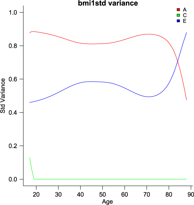
umxGxE_window (Briley et al., Reference Briley, Harden, Bates and Tucker-Drob2015) also implements a gene– environment interaction model. It does this not by imposing a particular function (linear or otherwise) on the interaction, but by estimating the model sequentially on windows of the data. In this way, it generates a spline-style interaction function that can take arbitrary forms (see Figure 11). The function linking genetic influence and context is not necessarily linear, but may react more steeply at extremes of the moderator, take the form of known growth functions of age, or take other, unknown forms. To avoid obscuring the underlying shape of the interaction effect, local structural equation modeling (LOSEM) may be used, and umxGxE_window implements this model. LOSEM is non-parametric, estimating latent interaction effects across the range of a measured moderator using a windowing function which is walked along the context dimension, and which weights subjects near the center of the window highly relative to subjects far above or below the window center. This allows detecting and visualizing arbitrary G × E (or C × E or E × E) interaction forms.
Output graphic from a windowed or ‘LOSEM’ G × age analysis.
Example G × E Windowed Analysis
We first need to set up the data correctly for the analysis. umxGxE_window takes a data.frame consisting of a moderator and two DV columns: one for each twin. The model also assumes two groups: MZ and DZ. Moderator cannot be missing, so to be explicit, we delete cases with missing moderator prior to analysis. The first three lines open the data set and define the name of the moderator column in the data set (‘age’ in this case), along with the DV (‘bmi’):
We next pull out the younger cohort from the data, remove rows where the moderator is missing and generate the MZ and DZ subsets of the data:
Next, we run the analysis:
The software reports to the user as it works through each level of the moderator encountered and produces a graph at the end of this run, plotting the A, C and E windowed estimates at each level of the moderator (see Figure 11). It is possible to run the function at only a single level or chosen range of moderator values, and of course the model results may be subjected to additional tests (Briley et al., Reference Briley, Harden, Bates and Tucker-Drob2015).
Summary
umx offers a variety of functions for rapid path-based modeling, a growing set of twin models, and helpful plotting and reporting routines. It makes available a set of data-processing functions, especially suitable for twin or wide-format data. Helping to lower the learning curve, a tutorial blog site operates at http://tbates.github.io. In addition, a help forum for users of the package is provided at the OpenMx website http://openmx.ssri.psu.edu/forums.
It is hoped that the package is useful not only to those learning and undertaking behavior genetics but also to the wider set of users seeking to utilize the power of structural modeling in their work and who seek approachable but powerful open-source solutions for this need.
Note: All example code in this paper available in the umx package as ?umxExamples.


 Open access