Introduction

During the austral summer of 1961–62 a seven-man party carried out geophysical and; Iaciological investigations on the 1,700 km. Antarctic Peninsula traverse in Ellsworth Land and the southern Antarctic Peninsula. Figures 1 and 2 show the area studied. Seismic measurements of ice thickness were made at 25 locations (Table 1 and Fig. 2) as discussed by Reference BehrendtBehrendt (1963). Velocity-depth curves were constructed by a method of numerical integration (Reference SlichterSlichter, 1932) using the time and distance data for the refracted compressional waves: raveling through the snow. A continuous velocity increase with depth was assumed to the iepth where maximum velocity is reached (about 150 m. in this area).

Fig. 1.

Map of Antarctica showing area studied

Fig. 2.

Surface elevation map showing location of major station (from Reference BehrendtBehrendt, 1963)

From these velocity-depth curves, density–depth curves were constructed using the f.mpirical expression Reference RobinRobin (1958, p. 88) showed to be valid below depths of 15 m.:

where ρ is the density in g./cm.³, V _p is the compressional wave velocity in m./sec., and T is the temperature in °C. Figures 3–7 show the results of these calculations using the temperatures at 10 m. (from H. Shimizu personal communication). The variations in these curves are probably the result of the wide range in annual accumulation values (20 to 50 g./cm.² yr.) since the standard deviation of the mean annual (10 m.) temperatures is only ±2.6° C. from the average of −22° C. This suggested a method of determining quantitative estimates of mean annual accumulation from the seismic data.

Fig. 3.

Density-depth curves stations 224–320

Fig. 4.

Density-depth curves stations 382–528

Fig. 5.

Density-depth curves stations 572–764

Fig. 6.

Density-depth carves stations 840–1028

Fig. 7.

Density-depth curves for 5 refraction stations extended to penetrate to depth of maximum velocity

Table 1.

Accumulation Determined From Seismic Data and Near-Surface Glaciology

Discussion

Pit measurements of accumulation values for twelve stations (Table 1), furnished the author by Shimizu, were used with a value for “Eights” station determined from one season’s observed snow accumulation. Figure 8 is a graph of accumulation A versus the density ρ at 40 m. depth. The straight line shown was fitted by least squares to the data and the standard deviation of the points is ±4.7 g./cm.² yr. in terms of accumulation. This graph shows an inverse relation between accumulation and the density at 40 m. at this relatively constant temperature.

Fig. 8.

Graph of accumulation vs. density at o m. depth. Straight line is the least-square fit through the data; curve is determined by the expression shown

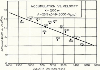
Another empirical study was carried out using the velocity vs. distance curves constructed directly from the travel-time curves. Figures 9–11 compare accumulation with compressional wave velocities recorded at distances of 50,100, and 200 m. from the shot point, respectively. Assuming linear relationships for these graphs also, the standard deviations in terms of measured accumulations from the least-square straight lines are ±6.0 g./cm.² yr., 5.8 g./cm.² yr., and ±4.5 g./cm.² yr. for 50,100, and 200 m. distances respectively. The depths h corresponding to the velocities at each of these distances X were measured and averaged from the velocity-depth curves with the following results: X = 50 m., h = 11 m., with standard deviation s = ±3.3 m., X = 100 m., h = 21 m., s = ±4.2 m., and X = 200 m., h = 41 m., s = ±2.7 m. The least scatter from the straight lines was for X = 200 m. (Fig. 11) corresponding to a mean depth of 41 m.; this is essentially equivalent to Figure 8 for accumulation versus density at 40 m. depth.

Fig. 9.

Graph of accumulation vs. compressional wave velocity observed 50 m. from the shot point. The straight line is the least-square fit to the data

Fig. 10.

Graph of accumulation vs. compressional wave velocity observed 100 m. from the shot point. The straight line is the least-square fit to the data

Fig. 11.

Graph of accumulation vs. compressional wave velocity observed 200 m. from the shot point. The straight line is the least-square fit to the data

I attempted an explanation of these empirical results on a theoretical basis. Reference BaderBader (1962) and Reference LandauerLandauer (1957) gave the following relations for the rate of snow densification (−v):

where t is the time, σ the load in

where ρ is the average density from the surface to a depth h, σ ₀ = 700 g./cm.²; and c is a constant depending on snow type and temperature. Thus

Integrating and rearranging gives

where k is a constant of integration. In the following discussion, I assumed k was also constant throughout the area studied. Using the 2 m. pit density data furnished by Shimizu and the density-depth curves of Figures 3–7, values of σ at 40 m. depth were calculated for each of the thirteen stations of Figure 8 by numerical integration. These were found to show the following apparently linear relation with ρ at 40 m. depth (Fig. 12):

Fig. 12.

Average density vs. density at 40 m. depth. The straight line is the least-square fit to the data

Using this expression introduced an error of ±0.9 per cent in ρ . Within the range of densities of Figure 8

or

with an introduced error ±0.4, per cent in 1/ρ. (The error introduced by the assumption a linear relation between 1/ρ and In ρ is less than that between ρ and In ρ in the density range from 0.7 to 0.8 g./cm.³.) From equation (6) and the relationship

a theoretical curve of cosh (σ/σ ₀) versus ln ρ was calculated and plotted on a graph of the observed data in Figure 13. The standard deviation of points from the curve is ±3.0 per cent and from the least-square fit of a straight line is ±2.7 per cent. Thus the approximation of the linear relationship

Fig. 13.

Graph cosh (σ/σ₀) vs. ln ρ. The straight line is the least-square fit to the data; the curve is the theoretical relationship

has an error of ±3 per cent.

Substituting equation (7) into equation (8) and substituting both into equation (5) gives:

Substituting the value of σ ₀ and solving for ρ this reduces to

with a combined error in ρ of ±3.4 per cent where ρ is in the range 0.7 to 0.8 g./cm.³. The best fit to the observed data was found to be c = 3.9×10⁻⁴ yr⁻¹ and.k = −0.42 These gave the expression

from which the curve of Figure 8 was drawn. The standard deviation from the observed data is ±6.8 g./cm.² yr. compared with ±4.7 g./cm.² yr. for the linear fit and ±4.5 g./cm.² yr. from. V _p at X = 200 (Fig. 11). Since a number of approximations and assumptions were made in deriving equation (10), it is not intended as a rigorous theoretical expression for the variation of density with accumulation. Rather, it allows some understanding of the empirical relations observed in Figures 8–11.

This discussion leads to the conclusion that at least in the area of the Antarctic Peninsula traverse, where the scatter in mean annual temperatures is small, the compressional wave velocity at 200 m. distance from the shot point or the density at 40 m. depth can be used to obtain reasonably reliable values of accumulation. The graph of accumulation versus velocity at 200 m. is preferred over the graph of accumulation versus density because it is much less time-consuming to determine a velocity (which can be taken directly from a seismogram) at a given distance than a density at a specific depth.

Determinations of the accumulation were made for all of the seismic stations as shown in Table 1 using Figures 8 and 11. A _L and A _C refer to values from the straight line and curve of Figure 8; A _V refers to the values from, V _p at X = 200 m. The standard deviation is ±2.9 g./cm.² yr. for the comparison of the three methods. This should be regarded as an indication of the internal agreement of the data rather than an indication of absolute accuracy of the accumulation values.

Acknowledgements

This work was conducted while the author was employed at the Geophysical and Polar Research Center at the University of Wisconsin and was supported by a grant from the National Science Foundation. I would like to thank C. R. Bentley for many helpful suggestions in the course of this study. This discussion, together with the velocity-distance-depth data, is included in Geophysical and Polar Research Center Report 64–1.