

1. Introduction
The extent of emerging markets’ (EMs) integration with world markets has been on the rise, especially when investors see investment in EMs as a way to diversify their portfolios to reduce risks (Divecha et al. Reference Divecha, Drach and Stefek1992; De Santis, Reference De Santis1993; Li et al. Reference Li, Sarkar and Wang2003; Berger et al. Reference Berger, Pukthuanthong and Yang2011). The analogy is that, as the EMs are considerably connected with the asset markets, their exchange rates are expected to be influenced by the simultaneous rise and fall of international asset prices and capital flows across countries in reaction to the varying financial conditions, the “global financial cycle.” This is in line with Verdelhan (Reference Verdelhan2018), who posit that the variations in exchange rates are significantly explained by global shocks.Footnote 1
Several push-pull factors, including country-specific indicators such as sentiments, risk rating, and political risk, have been shown to have contributed to deviation of market returns, currency depreciation, and reduction in all types of capital flows into emerging economies (Bekaert et al. Reference Bekaert, Erb, Harvey and Viskanta1998; Koepke, Reference Koepke2019; dos Santos et al. Reference dos Santos, Klotzle and Pinto2021).
The risk exposure of the EMs demands that risk-averse investors, especially, understand and reckon with the specific sentiments and risks associated with the EMs before jumping in. In contrast, De Bondt (Reference De Bondt1998) argues that just a few individual investors can understand these factors and other high-quality financial information. One of the medium investors who informs their personal risk assessment and investment decisions is to tap into public sentiment about EMs. This is buttressed by Brzeszczyński et al. (Reference Brzeszczyński, Gajdka and Kutan2015), who find public information or news as the main driver of asset prices.
Against this backdrop, the study seeks to ascertain a deeper understanding of the shock transmission of EMs and global sentiments and the global financial cycle on the EMs’ exchange rates. Our main aim is to analyze the interplay of global and domestic media sentiment and the global financial cycle concerning effects on the exchange rates. We look into both the nominal bilateral exchange rate against the United States dollar (USD)Footnote 2 and effective exchange rates (NEER). We contribute to the existing literature in three ways. Firstly, we propose a global sentiment factor for 95 economies using a dynamic factor model (DFM). We proceed to generate a symmetric effect model (baseline linear model) that explains the shock transmission mechanisms of EMs and global sentiments and the global financial cycle on the exchange rates. With the baseline model, we do not differentiate between positive and negative sentiments. We assume at this point that both positive and negative sentiments exert the same impact. That is, investors might respond to perceived opportunities or higher yields in EMs irrespective of sentiment polarity. To ascertain this, we apply the linear local projections put forward by Jordà (Reference Jordà2005).
As a second step, we investigate an asymmetric effect model (threshold model) associated with the shock transmission mechanisms. We adopt regime-switching models that employ the EMs sentiment, country-specific buzz, and monetary policies buzz to generate two separable states of “positive and negative sentiments,” “higher and lower buzzes,” and “higher and lower rates buzz.” In the next step, we assess how these states of the media perspectives distinctively interact with the global sentiment and global financial cycle to affect the EMs’ currencies. This helps us to explain investors’ behavior for investing in EMs. By analyzing the state of the intensity of the monetary policies discussed in the media, we contribute to the literature inspired by Miranda-Agrippino et al. (Reference Miranda-Agrippino, Nenova and Rey2020), who find that monetary policies affect the global financial cycle. It is important to stress that our asymmetric effect can stem from either the sign (direction) or the size (magnitude) of the shock impact on the exchange rates within the regimes. To achieve this, we use nonlinear local projections. Third, we contribute to Miranda-Agrippino and Ricco (Reference Miranda-Agrippino and Ricco2015) by filtering out the global economic fundamentals from their estimate of global factor and then generating the idiosyncratic component as our measure of “pure” global financial cycle shock. In this case, we are able to investigate the idiosyncratic shock of the global financial cycle on the exchange rates.
Given the prominent literature on textual analysis in these contemporary times, one of the major sources of public sentiment or information about the EMs is the news and social media outlets (Baker et al. Reference Baker, Bloom and Davis2016; Gui et al. Reference Gui, Kou, Pine and Chen2017; Michaelides et al. Reference Michaelides, Milidonis and Nishiotis2019). Public sentiment about the EMs or the global economy provides a broader picture of the country and global indicators that are expected to have a significant impact on the EMs’ asset returns and their domestic currencies. Shleifer and Summers (Reference Shleifer and Summers1990) point out that assets subject to the sentiment of EMs yield higher returns than assets that are not. This instigates a question of how the sentiments or perceptions of people about the EMs or the global economy could interact with the global financial cycle to affect EM currencies, which is relatively unexplored in the literature.
We analyze 17 EMs, including the most rapidly growing (G20) and other widely used EM currencies. As these economies continue to grow, they get linked to the global economy, making studying imperative. These economies’ new and social sentiments are extracted from Thomson Reuters Refinitiv MarketPsych Indices (TRMI). To have a comprehensive discussion, we dwell on the combined news and social media sentiments. For the global financial cycle, we employ the Miranda-Agrippino and Ricco (Reference Miranda-Agrippino and Ricco2015) and Miranda-Agrippino et al. (Reference Miranda-Agrippino, Nenova and Rey2020)’s global factor in risky asset prices, which summarizes the fluctuations in the global risky asset market prices, including equity prices, commodity prices, and corporate bond indices. The global factor is consistent with major worldwide events, as well as the United States (US) recession times as specified by the National Bureau of Economic Research (NBER) and also accounts for major changes in global risky asset prices. Following Passari and Rey (Reference Passari and Rey2015), we use the VIX index, which is a measure of risk aversion and uncertainty, as an additional proxy to examine the global financial cycle shock. The VIX co-moves with the global factor (Miranda-Agrippino and Rey, Reference Miranda-Agrippino and Rey2012; Rey, Reference Rey2013). According to Obstfeld et al. (Reference Obstfeld, Ostry and Qureshi2018), the VIX is highly correlated with the VXO index and provides similar results.
Our results illustrate a significant appreciation of the EMs’ currencies in response to shocks from the domestic and global sentiments and the general and pure global factors. By estimating two specifications of our factor model, we show that both global fundamentals and global risk have a significant impact on the exchange rates of emerging economies. VIX shock also leads to the depreciation of the EM currencies. We observe asymmetric effects with the degree of the domestic and global sentiments and the global financial cycles’ impacts on the EMs’ currencies being greater at the positive regime than at the negative regime. Moreover, the impact of domestic sentiments is magnified by higher country-specific and monetary policies’ media intensities. In contrast, global sentiments and global financial cycles exert a stronger impact on currencies in the lower country-specific and monetary policies’ media intensities regimes.
The remainder of this paper is as follows: section 2 elaborates on the related literature. Section 3 provides details of the data and the econometric methodology. Section 4 presents the empirical results, while an extension is made in section 5. Section 6 concludes.
2. Literature review
Our study relates to several strands of literature, which will be briefly summarized in the following. We start by briefly discussing determinants of EM currencies before summarizing studies that deal with the link between the Global Financial Cycle and Exchange Rates. Finally, we discuss the role of media sentiment as public information.
2.1 Currencies of emerging markets
Considering the determinants of EM currencies, the relationship between commodity prices and exchange rates has been considerably researched in the literature. Particularly, an enormous amount of studies have focused on the link between the oil price and the exchange rates of emerging markets with a focus on oil or commodity exporters (Basher et al. Reference Basher, Haug and Sadorsky2012; Delgado et al. Reference Delgado, Delgado and Saucedo2018; Roubaud and Arouri, Reference Roubaud and Arouri2018; Bai and Koong, Reference Bai and Koong2018; etc.). The relationship between oil prices and exchange rates is supported by strong theoretical reasoning, indicating a mutually reinforcing interaction in which oil price shocks affect exchange rate dynamics, and conversely, fluctuations in exchange rates can influence oil price movements, for example via trade or denomination channel (Beckmann et al. Reference Beckmann, Kerkemeier and Kruse-Becher2025). Overall, commodity currencies are often driven by specific commodity prices or commodity price uncertainty (Bermpei et al. Reference Bermpei, Ferrara, Karadimitropoulou and Triantafyllou2024).
Other studies which have focused on common factors in exchange rates have found that the G10 currency factors are less successful in explaining fluctuations in emerging market currencies which might reflect the stronger relevance of risk premia and uncertainty for emerging markets (Aloosh and Bekaert, Reference Aloosh and Bekaert2022).
2.2 Global financial cycle and exchange rates
The literature has long recognized that the currency and stock markets are closely related, since international investors face the risks of both the stock market and the exchange rate (Cenedese et al. Reference Cenedese, Payne, Sarno and Valente2016). Aloosh and Bekaert (Reference Aloosh and Bekaert2022) and Berg and Mark (Reference Berg and Mark2015) explain exchange rate fluctations via common factors, with the latter study illustrateing that third-country variables are significant predictors of bilateral exchange rate movements, showing the spillover effect from the rest of the world to a country’s currency. Another part of the literature explicitly investigates the impact of common variations in the global stock, bond, and commodity prices – the global financial cycle on the exchange rate. The last strand of literature to which our study relates focuses on the impact of the global financial cycle on exchange rates. Ranaldo and Söderlind (Reference Ranaldo and Söderlind2010), for example, employ a factor model to capture linear and nonlinear connections between currencies, stock and bond markets, as well as proxies for market volatility and liquidity. They illustrate that the Swiss franc and Japanese yen are safe havens as they appreciate against the USD when US stock prices decrease and US bond prices and FX volatility increase.
Besides, Kalra (Reference Kalra2011) uses GARCH models for global volatility (VIX and VDAX indices) on foreign exchange returns in East Asia and finds a shred of evidence for these exchange rates to depreciate with increases in global (equity) risk.
Studying the share of systematic variation in exchange rates, Verdelhan (Reference Verdelhan2018) also identify a strong impact of global shocks. Mollick and Sakaki (Reference Mollick and Sakaki2019) examine how 14 major currencies per USD respond to shocks from two global factors (oil and world equity returns). They find that commodity currencies strongly appreciate following positive oil price shocks and depreciate with positive global equity shocks. Eguren-Martin and Sokol (Reference Eguren-Martin and Sokol2022) apply quantile regression to study the relationship between exchange rate returns and global financial conditions. Their measure of global financial condition is related to Miranda-Agrippino and Ricco (Reference Miranda-Agrippino and Ricco2015). A recently study by Rey et al. (Reference Rey, Stavrakeva and Tang2024) provides an overarching perspective on the role of the global financial cycle for exchange rates. Their findings show that exchange rates are closely connected to the global network of equity holdings. They argue that exchange rates can be expressed as local currency stock market capitalization minus equity holdings, denominated in investors’ currencies and are also reflected by the “centrality” of currencies in global equity markets.
2.3 Media sentiment as public information and exchange rates
Theoretically, sentiment refers to the positive and negative tonality of the media coverage, which, when publicly available, provides information that affects the financial markets. This is in line with the efficient market hypothesis (EMH), which stipulates that the market responds quickly and correctly to all publicly available information, such as media sentiment. From a behavioral perspective, a strand of literature has examined the impact of sentiment on investor behavior and exchange rate dynamics (Michaelides et al. Reference Michaelides, Milidonis and Nishiotis2019; Filippou et al. Reference Filippou, Taylor and Wang2021; Kaourma et al. Reference Kaourma, Milidonis, Nishiotis and Panayides2025). Filippou et al. Reference Filippou, Taylor and Wang2021) examine media sentiment and currency reversals for 48 foreign exchange rates and conclude that currency reversals based on media sentiment exhibit a well-defined feature of the foreign exchange market. Also, Kaourma et al. (Reference Kaourma, Milidonis, Nishiotis and Panayides2025) investigate the trading behavior of individual investors using an intraday dataset of a pool of retail investors’ long and short positions in EUR/USD. Their findings indicate that retail investors are influenced by public information from news sentiment.
Investors attach sentiment to their investment in countries due to the level of risk and dispersion in the markets, which can eventually affect the dynamics of the country’s currency. In line with the impact of sentiment on the dynamics and dispersion of currencies, Plakandaras et al. (Reference Plakandaras, Papadimitriou, Gogas and Diamantaras2015) use sentiment from StockTwits posts to perform an out-of-sample forecast of the future direction of four exchange rates against the USD, showing the rejection of the EMH. Lehkonen et al. (Reference Lehkonen, Heimonen and Pukthuanthong2020) investigate the significance of media tone in predicting the exchange rate returns of 24 EMs using news and social media articles. Applying VAR-GARCH(1,1) to analyze the spillovers between the macro news and the exchange rates in the EMs, Caporale et al. (Reference Caporale, Spagnolo and Spagnolo2018) show limited dynamic linkages among the first moments related to the second moments and causality-in-variance observed in some cases. A recent study by Beckmann et al. (Reference Beckmann, Kerkemeier and Kruse-Becher2025), who examine temporary phases of exchange rate predictability in a two-regime threshold predictive regression framework, finds that phases of predictability are triggered by increased media coverage and high uncertainty.
Testing the asymmetric impact of public information from news sentiment, Laakkonen & Lanne, Reference Laakkonen and Lanne2009) examine how positive and negative macroeconomic US and European news announcements in various phases of the business cycle affect the high-frequency volatility of the EUR/USD exchange rate. They find that negative news increases volatility more in good times than in bad times. However, there is no difference between the volatility effects of positive news in bad and good times.Footnote 3 Also, Tetlock (Reference Tetlock2010) applies public financial news events and finds patterns in post-news returns and trading volumes consistent with asymmetric information models.
Some studies have adopted other sentiment measures in the context of exchange rates. Akhtar et al. (Reference Akhtar, Faff and Oliver2011) use the Consumer Sentiment Index (CSI) to examine the effect of consumer sentiment announcements on changes in 13 foreign exchange rates against the Australian dollar (AUD). Their results identify an asymmetric effect, in that an announcement of a lower or negative CSI leads to the depreciation of the AUD. However, no significant impact occurs when positive CSI is announced. Furthermore, Goddard et al. (Reference Goddard, Kita and Wang2015) measure investors’ active attention using the Google search volume index (SVI) and find that it co-moves with contemporaneous FX market volatility, suggesting that investor attention is a priced source of risk in FX markets.
Our study relates to the literature by diving deeper into the asymmetric effect of the media sentiment and attention (media buzz) paid to emerging countries and their interrelation with the global financial cycles, which has not been studied in the literature.
Looking into EMs, sentiment provides public information about the domestic and global economies, which affect risk appetite and global financial cycles. Brzeszczyński et al. (Reference Brzeszczyński, Gajdka and Kutan2015) find that public information drives asset prices. This theoretical link suggests that the interaction between these sentiments can influence the size and sign of the global financial cycle’s impact on the currencies of the EMs. Unfortunately, there are no empirical investigations that examine how the public information proxy by media sentiment affects the transmission of global financial cycle shocks into EM exchange rates. This is what the study seeks to address.
3. Data and methodology
3.1 Data
A balanced panel of 17 EMs, according to the International Monetary Fund (IMF) groupingFootnote 4 is examined with monthly data from January 1998 to April 2019.
We obtain country-specific sentiments and buzz data without inherent biases from Thomson Reuters Refinitiv MarketPsych Indices (TRMI). Michaelides et al. (Reference Michaelides, Milidonis and Nishiotis2019) use the same dataset as public information in the currency market. The TRMI employs lexical analysis to extract sentiment indices in real-time by reckoning several sources comprising conventional newspaper articles and social media platforms, such as Twitter, every minute, totaling over two million news articles and posts daily. MarketPsych has been given emerging attention in recent research since it generates a wider news and social media sentiment index by converting these volumes and professional news into manageable information flows that are capable of influencing decisions. The TRMI scores the news and social media content as sentiment indices, which are described as overall positive references, net of negative references. This is a bipolar ranging from −1 to 1, such that a positive score value in the bipolar is termed a positive opinion and a negative value shows a negative opinion and 0 refers to neutrality. The buzz is the number of words used to compute the sentiment index, representing the intensity of media attention to the economy.
We generate a global sentiment factor from 95 countries’ sentimentsFootnote 5 by applying a DFM as shown in the equation below (see Appendix A for details of this model):
 \begin{equation} x_{t}^{i} = \alpha _{{global}}^{x,i}\, f_{t}^{x, {global}} + e_{t}^{x,i} \end{equation}
where $x_{t}^{i}$
includes the sentiment for the respective 95 countries at month
$x_{t}^{i}$
includes the sentiment for the respective 95 countries at month $t$
.
$t$
. $f_{t}^{x, {global}}$
is the global common factors for the variables. This helps to integrate the impact of the co-movement factor among the global sentiments.
$f_{t}^{x, {global}}$
is the global common factors for the variables. This helps to integrate the impact of the co-movement factor among the global sentiments.
Although there have been several measures of the global financial cycle, we rely on the global factor estimated by Miranda-Agrippino and Ricco (Reference Miranda-Agrippino and Ricco2015), which has received more attention in the literature. This is also utilized in Miranda-Agrippino and Rey (Reference Miranda-Agrippino and Rey2020). The global factor explains a significant share of the common variation in a large cross-section of risky asset prices globally. Miranda-Agrippino and Ricco estimate the global factor using aDFM at monthly frequency data for a larger and an unbalanced (heterogeneous) panel of risky asset prices traded globally.Footnote 6 They use the log-returns of the asset prices.Footnote 7 These asset prices comprise equity prices covering Europe, North and Latin America, Asia Pacific, and Australia; commodity prices excluding precious metals; and corporate bond indices. This is then extended by Miranda-Agrippino et al. (Reference Miranda-Agrippino, Nenova and Rey2020) with two dimensions: time by estimating the data to cover up to April 2019 and cross-section, through including a larger and richer set of price series that is updated to reflect the relevant adjustments in global markets, especially via the inclusion of Chinese stocks. One of the advantages of using the global factor is that it accounts for major changes in global risky asset prices.Footnote 8
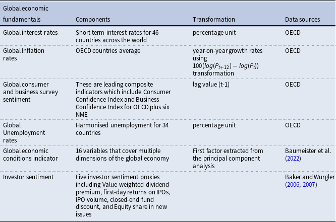
Furthermore, the impact of the global factor of risky assets could be influenced by global economic fundamentals, including interest rate, inflation, economic conditions indicator, consumer and business survey sentiments, investor sentiment, and unemployment rate. As with generating the global sentiment factor shown in Equation (1), we apply the DFM presented in Equation (2) to obtain common factors for the respective global economic fundamentals (see Table A2 in Appendix A for details on the data set of the global economic fundamental indicators).
 \begin{equation} y_{t}^{i} = \alpha _{{global}}^{y,i}\, f_{t}^{y, {global}} + v_{t}^{y,i} \end{equation}
where $y_{t}^{i}$
denotes the global economic fundamentals including the interest rate series, consumer and business survey sentiment and unemployment rates at month
$y_{t}^{i}$
denotes the global economic fundamentals including the interest rate series, consumer and business survey sentiment and unemployment rates at month $t$
.
$t$
. $f_{t}^{y, {global}}$
is the global common factors for the economic fundamentals.
$f_{t}^{y, {global}}$
is the global common factors for the economic fundamentals.
We filter out these global economic fundamental factors from the global factor proposed by Miranda-Agrippino and Ricco to generate a “pure” global factor shock. Sometimes we refer to Miranda-Agrippino and Ricco’s global factor as a “general global factor” to ensure a distinction from the “pure global factor shock.”
Rey (Reference Rey2015) identify VIX to co-move with the global financial cycle. To have a comparative analysis, we employ VIX as a proxy for the global financial cycle. VIX is the Chicago Board Options Exchange (CBOE) Volatility Index that measures market expectations with respect to volatility represented by the Standard & Poor 500 index option prices. This is usually used as a global financial market risk in the literature. In this case, we employ the direct measure of the global financial cycle by Miranda-Agrippino and Ricco and the VIX as an uncertainty measure. We retrieved VIX data from FRED, Federal Reserve Bank of St. Louis.Footnote 9
The target variable in our empirical analysis is the EM currencies, which, for robustness checks, we rely on both the nominal bilateral exchange rates against the USD and the effective exchange rates (broad indices).Footnote 10 Next, we measure the value of the currencies as the average log-returns of the exchange rates from the first day of the current month to the first day of the subsequent month, such that a decrease in the bilateral exchange rate and an increase in the effective exchange rate mean appreciation of the domestic currency and vice versa. We control for the economy’s macroeconomic indicators, such as the inflation rate and the industrial production index.Footnote 11 This helps factor in business cycle variation in the analysis. To ensure comparable units, we standardized the data variables employed in this study.
3.2 Methodology
We set the background by looking at the EMs and global sentiments and the global financial cycle shock transmission on the EMs’ currencies. To achieve this, we employ the local projection introduced by Jordà (Reference Jordà2005), which is less sensitive to misspecification and free from dynamic restrictions, giving us the flexibility to apply it to both linear and nonlinear models. This has been used in several studies, including Jordá and Taylor (Reference Jordà and Taylor2016), Ramey and Zubairy (Reference Ramey and Zubairy2018), etc. We begin our empirical analysis with the baseline specification by generating the impulse response for the linear local projection.
 \begin{align} FX_{j,t+h}^{i,Comp} = \alpha _{h} + \lambda _{j,h} + \sum _{k=1}^r \beta _{k,h}^{Comp}Sent_{j,t-k} + \sum _{k=1}^r \phi _{k,h}^{Comp}GSent_{t-k} + \sum _{k=1}^r \gamma _{k,h}^{Comp}GFact_{t-k} \nonumber \\ +\sum _{k=1}^r \chi _{k,h}^{Comp}FX_{j,t-k}^{i,Comp} + \sum _{k=1}^r \mu _{k,h}^{Comp}INF_{j,t-k} + \sum _{k=1}^r\delta _{k,h}^{Comp}IPI_{j,t-k} + \epsilon _{j,t+h}^{Comp}, \end{align}
where $FX_{j,t+h}^{i,Comp}$
is the cumulative log-returns of the bilateral or effective exchange rate for the country
$FX_{j,t+h}^{i,Comp}$
is the cumulative log-returns of the bilateral or effective exchange rate for the country $j$
. Our local projection coefficients of interest include
$j$
. Our local projection coefficients of interest include $\beta _{k,h}^{Comp}, \phi _{k,h}^{Comp}$
and
$\beta _{k,h}^{Comp}, \phi _{k,h}^{Comp}$
and $\gamma _{k,h}^{Comp}$
, giving the cumulative effect of the country-specific, that is, domestic sentiment (
$\gamma _{k,h}^{Comp}$
, giving the cumulative effect of the country-specific, that is, domestic sentiment ( $Sent_{j,t}$
), global sentiments (
$Sent_{j,t}$
), global sentiments ( $GSent_{t}$
) and the global financial cycle variables (
$GSent_{t}$
) and the global financial cycle variables ( $GFact_{t}$
), respectively, from time
$GFact_{t}$
), respectively, from time $t$
to
$t$
to $t+h$
for each element of the log-returns of the exchange rates. As stated earlier, shock transmission may be affected by economic fundamentals, especially the variation of the business cycle, to some extent. EMs with a suitable inflation and production growth track record influence their capacity to issue more securities in local currency (Burger and Warnock, Reference Burger and Warnock2007; Koepke, Reference Koepke2019). In this vein, we control for key domestic macroeconomic variables such as inflation (
$t+h$
for each element of the log-returns of the exchange rates. As stated earlier, shock transmission may be affected by economic fundamentals, especially the variation of the business cycle, to some extent. EMs with a suitable inflation and production growth track record influence their capacity to issue more securities in local currency (Burger and Warnock, Reference Burger and Warnock2007; Koepke, Reference Koepke2019). In this vein, we control for key domestic macroeconomic variables such as inflation ( $INF_{j,t}$
) and industrial production (
$INF_{j,t}$
) and industrial production ( $IPI_{j,t}$
).Footnote
12
Again, we include the lag of the exchange rates as control variables to develop auto-correlation, which accounts for the persistence in the realized monthly exchange rate. Additionally, we account for country-fixed effects,
$IPI_{j,t}$
).Footnote
12
Again, we include the lag of the exchange rates as control variables to develop auto-correlation, which accounts for the persistence in the realized monthly exchange rate. Additionally, we account for country-fixed effects, $\lambda _{j,h}$
.
$\lambda _{j,h}$
. $r$
is the lag of the variables employed in the system. We use 6-month lags; however, changing the number of lags does not significantly change the results. We perform a
$r$
is the lag of the variables employed in the system. We use 6-month lags; however, changing the number of lags does not significantly change the results. We perform a $h$
steps ahead forecast horizon, thus in this study we estimate the cumulative response of the exchange rates with robust standard errors up to 20 months ahead. The cumulative response provides a total effect of the exchange rate movement, thus capturing both temporary and long-run effects over time, making the study results relevant for policy implications. To ensure robustness of the standard error, we apply the Variance-Covariance matrix estimator, Spatial and Serial Correlation Consistent (vcovSCC). This helps to address the serially correlated, cross-sectional dependence and heteroskedasticity associated with the errors.
$h$
steps ahead forecast horizon, thus in this study we estimate the cumulative response of the exchange rates with robust standard errors up to 20 months ahead. The cumulative response provides a total effect of the exchange rate movement, thus capturing both temporary and long-run effects over time, making the study results relevant for policy implications. To ensure robustness of the standard error, we apply the Variance-Covariance matrix estimator, Spatial and Serial Correlation Consistent (vcovSCC). This helps to address the serially correlated, cross-sectional dependence and heteroskedasticity associated with the errors.
This baseline linear model discussed so far assumes that both positive and negative sentiments play the same role in the exchange rate response to shocks in the global sentiments and global financial cycle. Equation (3) tests three hypotheses: (i) both domestic and global sentiments cause both bilateral and effective exchange rates to appreciate such that higher sentiments appreciate the domestic currency and vice versa. (ii) An increase in the global risky asset market returns (global factor or pure global factor shock) causes the emerging economies’ currencies to appreciate in the short run due to the demand for the domestic currency to invest in EMs, which corresponds to the study by Ranaldo and Söderlind (Reference Ranaldo and Söderlind2010). (iii) The VIX shock leads to the depreciation of the currencies of emerging economies.
Investors may choose not only to invest in risky EM economies based solely on the global financial cycle, such as the returns on risky assets. They also perceive the value of risky assets by considering media sentiment or perceptions regarding specific EMs or the global economy to determine whether the investment is good or bad (Shiller, Reference Shiller1990). This demonstrates how EMs and global sentiments interact with the global financial cycle.
Positive vs. Negative News: The size or sign of sentiments and global financial cycle effects on the currency is expected to be influenced differently during positive and negative sentiment states of EM economies. Therefore, by analogy, we create a threshold country sentiment for positive and negative as below:
 \begin{equation} I_{t} = \begin{cases} 1 &{if}\, S_{t-1} \gt 0 \quad ({Positive}),\\ 0 &{if}\, S_{t-1} \leq 0 \quad ({Negative}). \end{cases} \end{equation}
where $S_{t-1}$
is the lag of the country sentiment.
$S_{t-1}$
is the lag of the country sentiment. $I_{t}$
is a dummy of 1 when it is a positive sentiment and otherwise it becomes a negative sentiment.
$I_{t}$
is a dummy of 1 when it is a positive sentiment and otherwise it becomes a negative sentiment.
High vs. Low Media Intensities: Another important analysis is to examine the interaction between the degree of media intensity, sentiments, the global financial cycle, and the EMs’ exchange rates. This helps to investigate how the level of media attention in the EMs influences sentiments and the impact of the global financial cycle on exchange rates. To do this, we employ the country-specific media buzz. We also contribute to Miranda-Agrippino and Rey (Reference Miranda-Agrippino and Rey2020) by looking into the monetary policies’ buzz, which is termed as rates buzz. The country-specific buzz, as media coverage explains the number of words used to compute the EMs’ sentiment indicators, which directly measures the country-specific media intensity. On the other hand, the monetary policies’ buzz is a sum of all references underlying the central bank, interest rates and their forecast values, debt defaults, and monetary policy loose and tight. We generate a threshold of higher and lower buzz:
 \begin{equation} I_{t} = \begin{cases} 1 &{if}\, Buzz_{t-1}^{i} \gt \overline {Buzz}^{i},\\[6pt] 0 &{if}\, Buzz_{t-1}^{i} \leq \overline {Buzz}^{i}, \end{cases} \end{equation}
where $Buzz_{t-1}^{i}$
measures the media attention given to the EMs at time
$Buzz_{t-1}^{i}$
measures the media attention given to the EMs at time $t-1$
and
$t-1$
and $I_{t}$
in Equation (5) refer to higher buzz (
$I_{t}$
in Equation (5) refer to higher buzz ( $HigherBuzz_{t-1}^{i}$
) where
$HigherBuzz_{t-1}^{i}$
) where $i$
denotes the country-specific buzz or monetary policies buzz.
$i$
denotes the country-specific buzz or monetary policies buzz. $\overline {Buzz}^{i}$
is the mean of the country-specific buzz or monetary policies’ buzz. A dummy 1 is given when the buzz at time
$\overline {Buzz}^{i}$
is the mean of the country-specific buzz or monetary policies’ buzz. A dummy 1 is given when the buzz at time $t-1$
is greater than the average buzz and we term it a higher buzz regime; otherwise, we denote it as a lower buzz regime. The higher buzz regime explains the higher media intensity, while the lower buzz regime represents the lower media intensity.
$t-1$
is greater than the average buzz and we term it a higher buzz regime; otherwise, we denote it as a lower buzz regime. The higher buzz regime explains the higher media intensity, while the lower buzz regime represents the lower media intensity.
In the second stage, we build on the baseline model by extending the local projection estimation with state-of-the-art regime switching as in Auerbach and Gorodnichenko (Reference Auerbach and Gorodnichenko2012), Ahmed and Cassou (Reference Ahmed and Cassou2016), Ramey and Zubairy (Reference Ramey and Zubairy2018), Cloyne et al. (Reference Cloyne, Jordà and Taylor2023), Gonçalves et al. (Reference Gonçalves, Herrera, Kilian and Pesavento2024), Inoue et al. (Reference Inoue, Rossi and Wang2024), etc. This state dependence explains the distinguished nonlinear response of exchange rates to sentiments and global financial cycle shocks when the emerging economy is in a state of positive or negative by incorporating Equation (4) into the local projection. This is represented by the regime-switching model in Equation (6). This specification describes the asymmetric impact of the sentiments, summarizing the different influences of positive and negative sentiment.Footnote 13
 \begin{align} FX_{j,t+h}^{i,Comp} &= I_{t}\Biggl [\alpha _{h}^{P} + \lambda _{j,h}^{P} + \sum _{k=1}^r \beta _{k,h}^{P,Comp}Sent_{j,t-k} + \sum _{k=1}^r \phi _{k,h}^{P,Comp}GSent_{t-k} + \sum _{k=1}^r \gamma _{k,h}^{P,Comp}GFact_{t-k} \nonumber \\ & \qquad+\sum _{k=1}^r \chi _{k,h}^{P,Comp}FX_{j,t-k}^{i,Comp} + \sum _{k=1}^r \mu _{k,h}^{P,Comp}INF_{j,t-k} + \sum _{k=1}^r\delta _{k,h}^{P,Comp}IPI_{j,t-k}\Biggr ] \nonumber \\ & \qquad+(1 - I_{t})\Biggl [\alpha _{h}^{N} + \lambda _{j,h}^{N} + \sum _{k=1}^r \beta _{k,h}^{N,Comp}Sent_{j,t-k} + \sum _{k=1}^r \phi _{k,h}^{N,Comp}GSent_{t-k} \nonumber \\ & \qquad + \sum _{k=1}^r \gamma _{k,h}^{N,Comp}GFact_{t-k} +\sum _{k=1}^r \chi _{k,h}^{N,Comp}FX_{j,t-k}^{i,Comp} \nonumber \\ & \qquad+ \sum _{k=1}^r \mu _{k,h}^{N,Comp}INF_{j,t-k} + \sum _{k=1}^r\delta _{k,h}^{N,Comp}IPI_{j,t-k}\Biggr ] + \epsilon _{j,t+h}^{T,Comp}, \end{align}
where $I_{t}$
denotes the threshold dummy variable.
$I_{t}$
denotes the threshold dummy variable. $P$
and
$P$
and $N$
added to the coefficients suggest positive or higher intensity and negative or lower intensity, respectively.
$N$
added to the coefficients suggest positive or higher intensity and negative or lower intensity, respectively. $\epsilon _{j,t+h}^{T,Comp}$
represents the error of the asymmetric model. The other notations remain the same as explained above. Equation (6) tests our fourth hypothesis that there is an asymmetrical impact of sentiments and the global financial cycle, which is in line with Laakkonen & Lanne, Reference Laakkonen and Lanne2009) and Akhtar et al. (Reference Akhtar, Faff and Oliver2011).
$\epsilon _{j,t+h}^{T,Comp}$
represents the error of the asymmetric model. The other notations remain the same as explained above. Equation (6) tests our fourth hypothesis that there is an asymmetrical impact of sentiments and the global financial cycle, which is in line with Laakkonen & Lanne, Reference Laakkonen and Lanne2009) and Akhtar et al. (Reference Akhtar, Faff and Oliver2011).
4. Empirical results
4.1 Linear analysis
4.1.1 Sentiments, Global Factor, and Exchange Rates
This section presents the combined news and social domestic and global sentiments and a “general” global factor shocks on the emerging economies’ currencies: nominal bilateral and effective exchange rates. We begin with the cumulative impulse response for the local projection for the baseline model (symmetric model) (Blue solid line) and continue with the asymmetric model (Blue and Red solid lines for positive and negative sentiment regimes, respectively).
As an empirical starting point, we present the cumulative impulse responses of the baseline model (symmetric model) for bilateral and effective exchange rates in Figures 1 and 2 with 95% confidence bands. The bilateral exchange rate against the USD appreciates significantly by 2% on impact until the second month following the shock of the media sentiments about the corresponding emerging economies. With the same sentiment shock, the effective exchange rate appreciates significantly by 4%. The results imply a general appreciation of the currencies in emerging economies and no strong differences between bilateral and effective exchange rates. The implication is that the sentiment about EMs provides public information and projects a good perception to investors who respond to investing in EMs. Positive (negative) news causes the domestic currency to appreciate (depreciate) in the short run as the demand for the currency increases (decreases).
Nominal bilateral exchange rate linear response to sentiments and global factor shocks.Note: This figure presents the linear response of the bilateral exchange rate to sentiments and global factor shocks. The shaded area represents the 95% confidence bands. Sentiment and Glo_Sentiment denote country-specific and global sentiments.

Nominal effective exchange rate linear response to sentiments and global factor shocks. Note: This figure presents the linear response of the effective exchange rate to sentiments and global factor shocks. The shaded area represents the 95% confidence bands. Sentiment and Glo_Sentiment denote country-specific and global sentiments.

At the same time, a shock from the global factor, which explains a significant share of the common variation in a large cross-section of global risky asset prices, causes the bilateral exchange rate to appreciate by about 1.5% on impact, while the effective exchange rate appreciates by around 0.7% until the second month. This shows a short-run appreciation of the EMs’ currencies in response to the global financial cycle shock. This is consistent with Mollick and Sakaki (Reference Mollick and Sakaki2019), who find that emerging currencies appreciate when there is a positive oil price shock and global equity. The economic implication is that investors respond to an increase in risky asset prices by investing in EMs. The demand for emerging currencies increases and starts to appreciate in the short run. The result is also in line with the appreciation of the dollar in times of global uncertainty.
4.2 Sentiments, “Pure” Global Factor Shock, and Exchange Rates
Next, we examine the idiosyncratic shock of the global factor, which we refer to as the pure global factor shock. The global factor estimated by Miranda-Agrippino and Ricco (Reference Miranda-Agrippino and Ricco2015), which is a common factor of global risky assets return, including equities, commodity prices, and bonds, can be influenced or soiled by a wide range of economic fundamentals. This provides a ground for one to question that the shock from the “general” global factor, as discussed in section 4.1.1, cannot differentiate between a pure shock component and common economic fundamental variations. We address this issue by screening out possible economic fundamentals. Thus, we estimate the pure global factor shock using the following steps:
First, following the literature, we identify a series of global fundamentals that largely influence the global financial cycle. For instance, global interest rates are considered risk-free rates in the financial market. We also include inflation rates, which have diverse impacts on risky asset returns. One is that central banks respond to higher inflation through contractionary policies, leading to a decrease in global factor (Miranda-Agrippino and Rey, Reference Miranda-Agrippino and Rey2020). In addition, inflation rates affect the real value of risky assets, such that higher inflation rates can cause the real value of risky assets to decrease. The other issue is that when rising global inflation is associated with higher nominal returns on risky assets such as stocks and commodities, investors may demand more risky assets to hedge against devaluing money. Another fundamental variable that we tend to consider is the indicators of economic conditions measured by Baumeister et al. (Reference Baumeister, Korobilis and Lee2022) to forecast real oil prices and global petroleum consumption. These indicators capture aggregate demand, which has an impact on risky assets.
Moreover, we consider the consumer and business survey sentiments, which indicate future household and business developments concerning production, orders, and stocks of finished goods. These factors can influence investors’ expectations and eventually affect risky asset returns. This global survey sentiment factor is good for monitoring output growth and adjustment in economic activities. Furthermore, we incorporate a proxy for investor sentiment used by Baker and Wurgler (Reference Baker and Wurgler2006) and (Reference Baker and Wurgler2007), which can predict changes in investor demand for risky assets. Positive investor sentiment is expected to reduce the global factor (risky asset returns). We eventually include unemployment rates as an economic health indicator, where a higher rate leads to a decline in risky assets. With these variables, we have provided a broader spectrum of global economic fundamentals that provide insight into or are influential on the demand and supply of global risky assets, which perhaps may directly or indirectly affect global risky asset returns.
In our next step, we apply the DFM represented in Equation (2) on these global series to extract a single factor for the individual economic fundamentals. In our third step, we regress the global factor on global economic fundamentals as follows:
 \begin{align} GlobalFactor_{t} = \alpha _{0} + \alpha _{1}GINT_{t} + \alpha _{2}GIFL_{t} + \alpha _{3}GEA_{t} + \alpha _{4}GBS_{t} + \alpha _{5}INMS_{t} + \alpha _{6}GUEP_{t} + \epsilon _{t}, \nonumber \\[3pt] \end{align}
where $GINT$
denotes the global interest rate factor;
$GINT$
denotes the global interest rate factor; $GIFL$
is the global inflation rate factor;
$GIFL$
is the global inflation rate factor; $GEA$
is the global economic conditions indicator;
$GEA$
is the global economic conditions indicator; $GBS$
represents global consumer and business survey sentiment factors;
$GBS$
represents global consumer and business survey sentiment factors; $INMS$
is the investor sentiment;
$INMS$
is the investor sentiment; $GUEP$
indicate the global unemployment rate.
$GUEP$
indicate the global unemployment rate. $\alpha _{i}$
are the parameters.
$\alpha _{i}$
are the parameters.
From Equation (7), we decompose the global factor shock into “expected shock,” also referred to as systematic shock (explained by the economic fundamentals) and “pure shock,” which we term as an idiosyncratic component ( $\epsilon _{t}$
). We are very interested in the pure shock because investors often respond to this shock to adjust their beliefs about the risky asset markets. We further proceed to measure the pure shock by estimating the autoregressive model of order one (AR(1)) of
$\epsilon _{t}$
). We are very interested in the pure shock because investors often respond to this shock to adjust their beliefs about the risky asset markets. We further proceed to measure the pure shock by estimating the autoregressive model of order one (AR(1)) of $\epsilon _{t}$
in Equation (7) below,
$\epsilon _{t}$
in Equation (7) below,
 \begin{equation} \epsilon _{t} = \beta _{0} + \beta _{1}\epsilon _{t-1}+ \omega _{t}, \end{equation}
and employ the error term, $\omega _{t}$
as the “pure global factor shock.” The trend of the pure global factor shock relative to the general global factor is illustrated in Figure
A1. We then put pure global factor shock into Equations (3) and (6) to estimate its interaction with the EMs and global sentiments and their shocks on the currencies.
$\omega _{t}$
as the “pure global factor shock.” The trend of the pure global factor shock relative to the general global factor is illustrated in Figure
A1. We then put pure global factor shock into Equations (3) and (6) to estimate its interaction with the EMs and global sentiments and their shocks on the currencies.
Nominal bilateral exchange rate linear response to sentiments and pure global factor shocks. Note: This figure presents the linear response of the effective exchange rate to sentiments and pure global factor shocks. The shaded area represents the 95% confidence bands. Sentiment and Glo_Sentiment denote country-specific and global sentiments.

Nominal effective exchange rate linear response to sentiments and pure global factor shocks. Note: This figure presents the linear response of the effective exchange rate to sentiments and pure global factor shocks. The shaded area represents the 95% confidence bands. Sentiment and Glo_Sentiment denote country-specific and global sentiments.

The baseline impulse responses are displayed in Figures 3 and 4. We observe that the shock transmissions of EMs sentiments to the exchange rates remain the same as discussed in section 4.1.1. An intuitive result is that filtering out the global macroeconomic fundamentals from the global factor enhances the significant impact of global sentiments and reduces the global financial cycle shock. Both the bilateral and effective exchange rates significantly appreciate on the impact of the global sentiment shock until the second month. The shock of pure global factor causes the bilateral and effective exchange rates to appreciate by 0.5% and about 0.2%, respectively, on impact until the second month and in the seventh month. However, compared to the general global factor in the earlier discussion, the degree of impact is reduced.
The significance of both the pure global factor and general global factor shocks implies confidence in the prevailing strength of the global economy, where substantial global economic conditions increase capital flows into EMs. As capital flows into emerging economies increase, investors can demand the domestic currencies of emerging economies, leading to the appreciation of their currencies.
4.3 Nonlinear analysis
4.3.1 Positive vs. negative
In the next step, we present the asymmetric impact emanating from the state-dependent positive and negative sentiments about the EMs in Figures 5 and 6 with the Blue and Red solid lines for positive and negative sentiments regimes, respectively.
Nominal bilateral exchange rate response to sentiments and global factor shocks: positive Vs. negative. Note: This figure presents the regime-switching impulse-response for the local projection of positive sentiment (Blue solid line) and the negative sentiment (Red solid line). The shaded area represents the 95% confidence bands. Sentiment and Glo_Sentiment denote country-specific and global sentiments.

Nominal effective exchange rate response to sentiments and global factor shocks: positive Vs. Negative. Note: This figure presents the regime-switching impulse-response for the local projection of positive sentiment (Blue solid line) and the negative sentiment (Red solid line). The shaded area represents the 95% confidence bands. Sentiment and Glo_Sentiment denote country-specific and global sentiments.

The first asymmetry we observe is that EMs’ sentiment shock causes the bilateral exchange rate to appreciate significantly until the second month in the positive regime, while there is no significant impact in the negative regime. This explains the asymmetric effect of the countries’ sentiments. We do not observe such a difference for the effective exchange rates, where a sentiment shock leads to a significant appreciation in both regimes. The effects of global sentiment also seem to be slightly more relevant for bilateral exchange rates in the positive regime.
Overall, the persistence of the sentiment across the regimes statistically suggests that there may not be an asymmetry or a nonlinear impact concerning the directional impact on the effective exchange rate in the short term, however, an asymmetric impact is observed with regard to the magnitude of impact. The EMs’ sentiments appreciate the currencies more strongly in the positive regime, with no significant effect in the negative regime. This confirms Shleifer and Summers (Reference Shleifer and Summers1990), where the appreciation of the currencies supports the relevance investors give to positive sentiment. As these EMs are regarded as highly volatile and risky, the results suggest that policymakers in these regions pay attention to the news sentiment and work towards projecting positive sentiment. This induces investors to invest more in the economy and eventually appreciate the domestic currencies.
In response to the global sentiment shock, the bilateral exchange rates appreciate significantly in the third month in the negative regime while the effective exchange rates appreciate in the second, eleventh and nineteenth months at the positive regime, as occurs in the baseline model.
Nominal bilateral exchange rate response to sentiments and global factor shocks: country-specific buzz. Note: This figure presents the regime-switching impulse-response for the local projection of higher buzz (Blue solid line) and the lower buzz (Red solid line). The shaded area represents the 95% confidence bands. Sentiment and Glo_Sentiment denote country-specific and global sentiments.

Nominal effective exchange rate response to sentiments and global factor shocks: country-specific buzz. Note: This figure presents the regime-switching impulse-response for the local projection of higher buzz (Blue solid line) and the lower buzz (Red solid line). The shaded area represents the 95% confidence bands. Sentiment and Glo_Sentiment denote country-specific and global sentiments.

As illustrated in Figures 5 and 6, the bilateral exchange rates appreciate significantly in both positive and negative regimes within the short run following the global factor shock. In response to similar shock, the effective exchange rates appreciate on impact until the third month in the positive regime, whereas there is a less significant effect in the negative regime. Comparatively, the impact of the global financial cycle is magnified more by the bilateral exchange rate against the USD than with the EMs’ effective exchange rates. This explains the US dollar effect. The implication could be that due to the lower interest rates in the US economy, a positive shock in global assets pushes portfolio capital to EMs, particularly bond markets, which causes EM currencies to appreciate over the US dollar (Koepke, Reference Koepke2019).
Again, the impact of the EMs’ sentiments and pure global factor shocks remains the same in both the positive and negative regimes, as explained in section 4.1.1. Moreover, the pure global factor shock significantly appreciates the effective exchange rate in the short run in both regimes (see Figures B1 and B2 in Appendix B for the results).
4.3.2 High vs. low media intensities
Country-Specific Media Intensity: The EMs’ sentiment, global sentiment and the global financial cycle impact on the exchange rates within the regime-switching of the country-specific buzz are reported in Figures 7 and 8 (see Figures B3 and B4 in Appendix B for the illustrations for the pure global factor shock). We observe that a shock from the EMs’ sentiment, global sentiment, and the general and pure global factor leads to a significant appreciation in the bilateral and effective exchange rates in both the higher and lower country-specific buzz regimes. However, there are exceptional cases where the global sentiment and pure global factor shock do not have a significant impact on the effective exchange rate in the higher buzz regime. Thus, we observe that the global sentiment, general and pure global factors, are more impactful in the lower buzz regime than at the higher buzz regime. This implies that the global financial cycle and global sentiment interact with the lower media intensity in the EMs and largely appreciate the EMs’ currencies than when the media intensity in the EMs is high. One explanation for stronger effects in the case of low coverage is that stronger media coverage can occur in times of high uncertainty. Another possibility might be that, in a low buzz environment, perhaps investors feel safer investing in EMs. These results are consistent with Goddard et al. (Reference Goddard, Kita and Wang2015), who find that investor attention affects the volatility in exchange rate markets.
Monetary Policies’ Media Intensity: Next, we follow Miranda-Agrippino and Rey (Reference Miranda-Agrippino and Rey2020) to examine how the monetary policies’ media intensity as a regime-switching variable influences the EMs’ sentiment, global sentiment and the global financial cycle impact on the exchange rates. To measure the monetary policies’ media intensity, we employ rates buzz which is a sum of all references underlying the central bank, interest rates and their forecast values, debt defaults and monetary policy loose and tight (see Figures 9 to 10). We observe that both the bilateral and effective exchange rates appreciate in response to the EMs’ sentiments, general global factor and pure global factor shocks, respectively, in both higher and lower rates buzz regimes.Footnote 14 There is an asymmetric effect where EMs’ sentiment impact is intensified at the higher rates buzz regime, thus higher monetary policies’ media intensity, while the global factor shock is boosted at the lower rates buzz regime, lower monetary policies’ media intensity. This supports Miranda-Agrippino and Rey (Reference Miranda-Agrippino and Rey2020) who find that the global factor declines in response to a contractionary US monetary policy shock. It is also in line with theory since the lower rates regime implies monetary policy loose in the EMs, hence, at this regime higher global factors (i.e., common movement in higher returns on risky assets) in the EMs become incentives for investors, leading to increasing capital inflow and eventually appreciation of the EMs’ currencies.
Nominal bilateral exchange rate response to sentiments and global factor shocks: monetary policies buzz. Note: This figure presents the regime-switching impulse-response for the local projection of higher interest rate buzz (Blue solid line) and the lower interest rate buzz (Red solid line). The shaded area represents the 95% confidence bands. Sentiment and Glo_Sentiment denote country-specific and global sentiments.

Nominal effective exchange rate response to sentiments and global factor shocks: monetary policies buzz. Note: This figure presents the regime-switching impulse-response for the local projection of higher interest rate buzz (Blue solid line) and the lower interest rate buzz (Red solid line). The shaded area represents the 95% confidence bands. Sentiment and Glo_Sentiment denote country-specific and global sentiments.

The results suggest that the reaction of EM currencies to global media sentiment shocks varies depending on the prevailing buzz or intensity of the monetary policy rates. Following a global sentiment shock, the bilateral exchange rate appreciates significantly at the higher rates buzz regime, with no significant impact at the lower rates buzz regime. In contrast, in a similar shock, the effective exchange rate appreciates in the lower rates buzz regime. This can be attributed to the fact that increased media buzz around higher rates typically signals tighter monetary policy, which might attract foreign investment due to higher expected returns in those EMs. This inflow of capital increases the demand for EM currencies, driving up their value relative to the US dollar. Overall, the results align with the results by Beckmann et al. (Reference Beckmann, Kerkemeier and Kruse-Becher2025), who also find that periods of exchange rate predictability can be triggered by high buzz.
In order to link these results to our previous empirical results, which have shown that positive sentiment tends to have stronger effects compared to negative sentiment, and to the importance of media intensity, we have considered simple correlations between buzz and sentiment provided in Table A1. It becomes apparent that Ratesbuzz and USbuzz display a clear positive correlation with positive sentiment for the corresponding economy and global sentiment. This suggests that the intensity of the media coverage might act as a propagation mechanism for the observed effect of positive coverage.
5. Extensions
5.1 VIX as an alternative measure of global financial cycle
Several studies have employed VIX as a proxy of the global financial cycle. Rey (Reference Rey2015) argue that the global financial cycle co-moves with VIX. Hence, we compare the impact of Miranda-Agrippino and Ricco (Reference Miranda-Agrippino and Ricco2015) and Miranda-Agrippino et al. (Reference Miranda-Agrippino, Nenova and Rey2020)’s global factor in risky asset prices with the VIX as an uncertainty measure. The global factor measured by Miranda-Agrippa and Ricco serves as the asset price channel through which the global financial cycle affects exchange rates, and VIX provides a channel through which risk aversion or uncertainty influences exchange rates. In this section, we measure the global financial cycle by using the continuous monthly VIX average at the level that is consistent with Ligonniere (Reference Ligonniere2018), Avdjiev et al. (Reference Avdjiev, Bruno, Koch and Shin2019), Cerutti et al. (Reference Cerutti, Claessens and Rose2019), Cunha et al. (Reference Cunha, Haines and Da Silva2019), Akdi et al. (Reference Akdi, Varlik and Berument2020), etc.
The sentiments and VIX shocks on the exchange rate impulse responses are displayed in Figures C1, C2, C3, C4, C5, C6 and C7 and C8 in Appendix C. Compared to section 4, we observe that VIX negatively co-moves with the global factor either the general or pure shock with respect to their impact on the exchange rate, which is consistent with Ligonniere (Reference Ligonniere2018) and Cerutti et al. (Reference Cerutti, Claessens and Rose2019). EMs and global sentiments maintain their effect on the EMs’ currencies. VIX shock causes the bilateral and effective exchange rates to depreciate significantly, suggesting depreciation of the EMs’ currencies. This is consistent with Kalra (Reference Kalra2011) and Agyapong (Reference Agyapong2023), who find mature market equity volatility and world uncertainty depreciating the exchange rate. The EMs’ currencies’ depreciating impact of VIX is similar in both positive and negative regimes, higher and lower country buzz regimes and higher and lower rates buzz.
The shock intensifies in both the negative sentiment and the lower country-specific and rates buzz regimes. Also, comparing the two exchange rates, the shock is more magnified with the bilateral exchange rates against the US dollar. The implication is that unfavorable US monetary policy increases VIX (market volatility), which affects financial variables and assets that flow into emerging economies (Nier et al. Reference Nier, Sedik and Mondino2014). During such global financial risk and higher uncertainty, risk-averse investors tend to sell risky stocks and demand the safe haven of the US dollar.
5.2 Global Sentiment, Global Factor, and US Dollar Sentiment
Considering the dominance of the US dollar, especially a key pricing currency in these international markets, we proceed to examine the relations between global sentiments, global factor and the US dollar sentiment. The results are reported in Figures D1 and D2. We observe a positive interrelation between the global sentiments, USD sentiment and the global factor. A shock in global sentiment leads to a positive media sentiment about the USD and an increase in the global factor, thus appreciation of the risky assets. Similarly, global sentiment and USD sentiment respond to global factor shocks by rising beyond the steady state. We find that on impact, global sentiment and global factor rise to the USD sentiment shock.
6. Summary and concluding remarks
This paper has added nuance to the shock transmissions of the EMs and global sentiments and the global financial cycle. We have distinguished between a “general” global factor and a “pure” global factor, which summarizes the global risky asset market returns and VIX on the EMs’ currencies. In a second step, we have analyzed the interplay of global and domestic media sentiment and the global financial cycle with regard to effects on the EM exchange rates based on both linear and nonlinear local projections put forward by Jordà (Reference Jordà2005).
We find a significant appreciation of the EMs’ currencies in response to shocks from domestic and global sentiments, and the general and pure global factors (risky asset prices). This is consistent with Mollick and Sakaki (Reference Mollick and Sakaki2019). The significant impact of the global factor supports that investors invest in EMs for higher returns as they seek to diversify their portfolios. In contrast, VIX shock leads to the depreciation of the EMs’ currencies against the US dollar. This confirms the US dollar being a “safe-haven” currency while emerging currencies are “risky” currencies (Ranaldo and Söderlind, Reference Ranaldo and Söderlind2010; Habib and Stracca, Reference Habib and Stracca2012).
We have also observed asymmetric effects with regard to the effect of domestic and global sentiments and the global financial cycles on the currencies of EMs. We find that the effects of domestic sentiment tend to be stronger in the case of positive media coverage. To a lesser extent, the impact of domestic sentiments is magnified at the higher country-specific and monetary policies’ media intensities.
Our results confirm that sentiments shift in different environments (such as different phases of the financial cycle, together with its pure version) and movements in the VIX are important determinants of exchange rates. This implies that policymakers should pay close attention to media sentiments, which also offer a potential transmission channel for policy communication. Emerging economies can, for example, formulate effective and stable economic policy measures that would generate positive sentiment, making these economies more appealing to investors.
Future research could analyze the transmission mechanisms of media coverage in greater detail. This could, for example, be done in the context of capital flow dynamics at the country level.
Declarations of interest
None.
Appendices
Appendix A
Linear correlation with the bilateral exchange rate

Note: The table reports the correlation estimates. $Bi\_FX$
is bilateral exchange rate;
$Bi\_FX$
is bilateral exchange rate; $Sent$
is sentiment;
$Sent$
is sentiment; $Pos$
is positive;
$Pos$
is positive; $Neg$
is negative;
$Neg$
is negative; $Glo\_Sent$
is global sentiment;
$Glo\_Sent$
is global sentiment; $Glo\_factor$
is global factor (global financial cycle).
$Glo\_factor$
is global factor (global financial cycle).
Dynamic factor model
Given $x_{t}$
denoting
$x_{t}$
denoting $n\times 1$
vector of observed series at time
$n\times 1$
vector of observed series at time $t$
:
$t$
: $(x_{1,t},\ldots ,x_{nt})^{\prime }$
in the case of this study it representing the 95 countries sentiments or the various global economic fundamentals (the global interest rate series, global consumer and business survey sentiment, proxies for investor sentiment and global unemployment rate) with
$(x_{1,t},\ldots ,x_{nt})^{\prime }$
in the case of this study it representing the 95 countries sentiments or the various global economic fundamentals (the global interest rate series, global consumer and business survey sentiment, proxies for investor sentiment and global unemployment rate) with $n$
number of series in
$n$
number of series in $x_{t}$
which contains
$x_{t}$
which contains $r$
number of factors and
$r$
number of factors and $p$
number of lags in factor VAR as the arguments to the DFM. A DFM can be estimated first by using the measurement or observation equation below:
$p$
number of lags in factor VAR as the arguments to the DFM. A DFM can be estimated first by using the measurement or observation equation below:
 \begin{eqnarray} x_{t} = \lambda F_{t} + \epsilon _{t}, \sim N(0,\Sigma _{\epsilon }) \end{eqnarray}
where $F_{t}$
represents
$F_{t}$
represents $r\times 1$
vector of factors at time
$r\times 1$
vector of factors at time $t$
:
$t$
: $(\,f_{1,t},\ldots ,f_{rt})^{\prime }$
.
$(\,f_{1,t},\ldots ,f_{rt})^{\prime }$
. $\lambda$
is
$\lambda$
is $n\times r$
measurement (observation) matrix or a vector of factor loadings.
$n\times r$
measurement (observation) matrix or a vector of factor loadings. $\epsilon _{t}$
is the
$\epsilon _{t}$
is the $n\times 1$
idiosyncratic measurement (observation) errors and
$n\times 1$
idiosyncratic measurement (observation) errors and $\Sigma _{\epsilon }$
gives
$\Sigma _{\epsilon }$
gives $n\times n$
measurement (observation) covariance matrix which by assumption is diagonal that follows
$n\times n$
measurement (observation) covariance matrix which by assumption is diagonal that follows $E[x_{it}|x_{-i,t},x_{1,t-i},\ldots ,f_{t},f_{t-1},\ldots ] = \lambda f_{t}\forall i$
. The factors are assumed to follow a VAR given a transition or state equation as:
$E[x_{it}|x_{-i,t},x_{1,t-i},\ldots ,f_{t},f_{t-1},\ldots ] = \lambda f_{t}\forall i$
. The factors are assumed to follow a VAR given a transition or state equation as:
 \begin{eqnarray} F_{t} = \sum _{i=1}^{p}\delta _{i}F_{t-i} + e_{t}, \sim N(0,Q_{0}) \end{eqnarray}
where $\delta _{i}$
represents
$\delta _{i}$
represents $r\times r$
state transition matrix at lag
$r\times r$
state transition matrix at lag $i$
and
$i$
and $Q_{0}$ $r\times r$
state covariance matrix. To ensure an efficient estimate, we set the dynamic factor model to pursue the following assumption (i)
$r\times r$
state covariance matrix. To ensure an efficient estimate, we set the dynamic factor model to pursue the following assumption (i) $x_{t}$
must be stationary, hence we transform all the series to be stationary before applying the DFM. (ii) there is no direct connection between the series and lagged factors or (iii) there is no serial correlation, that is, no relationship between the lagged error terms in either the measurement or transition equation. We apply information criteria to select the optimal lag and proceed to apply the principal component analysis (PCA) to determine the optimal number of factors needed to estimate the DFM. Several studies advocate the use of maximum likelihood to estimate the factors from DFM. For instance, Sentana and Shah (Reference Sentana and Shah1994) argue that when the series are non-Gaussian, the Gaussian Quasi-Maximum Likelihood (QML) efficiently estimates the static exact factor models. Hence, the maximum likelihood is preferable to principal components. Doz and Lenglart (Reference Doz and Lenglart1999) have examined the properties of QML estimators in a dynamic exact factor model in the case of serial correlation omission in the approximating model. Following Doz et al. (Reference Doz, Giannone and Reichlin2012), we eventually employ the Quasi-Maximum Likelihood (QML) to extract factor estimates from the DFM.
$x_{t}$
must be stationary, hence we transform all the series to be stationary before applying the DFM. (ii) there is no direct connection between the series and lagged factors or (iii) there is no serial correlation, that is, no relationship between the lagged error terms in either the measurement or transition equation. We apply information criteria to select the optimal lag and proceed to apply the principal component analysis (PCA) to determine the optimal number of factors needed to estimate the DFM. Several studies advocate the use of maximum likelihood to estimate the factors from DFM. For instance, Sentana and Shah (Reference Sentana and Shah1994) argue that when the series are non-Gaussian, the Gaussian Quasi-Maximum Likelihood (QML) efficiently estimates the static exact factor models. Hence, the maximum likelihood is preferable to principal components. Doz and Lenglart (Reference Doz and Lenglart1999) have examined the properties of QML estimators in a dynamic exact factor model in the case of serial correlation omission in the approximating model. Following Doz et al. (Reference Doz, Giannone and Reichlin2012), we eventually employ the Quasi-Maximum Likelihood (QML) to extract factor estimates from the DFM.
Global economic fundamental indicators
Global factor and pure global factor shock.

Appendix B: Pure global factor shock and asymmetric results
Nominal bilateral exchange rate response to sentiments and pure global factor shocks: positive Vs. negative. Note: This figure presents the regime-switching impulse-response for the local projection of positive sentiment (Blue solid line) and the negative sentiment (Red solid line). The shaded area represents the 95% confidence bands. Sentiment and Glo_Sentiment denote country-specific and global sentiments.

Nominal effective exchange rate response to sentiments and pure global factor shocks: positive Vs. negative. Note: This figure presents the regime-switching impulse-response for the local projection of positive sentiment (Blue solid line) and the negative sentiment (Red solid line). The shaded area represents the 95% confidence bands. Sentiment and Glo_Sentiment denote country-specific and global sentiments.

Nominal bilateral exchange rate response to sentiments and pure global factor shocks: country-specific buzz. Note: This figure presents the regime-switching impulse-response for the local projection of higher buzz (Blue solid line) and the lower buzz (Red solid line). The shaded area represents the 95% confidence bands. Sentiment and Glo_Sentiment denote country-specific and global sentiments.

Nominal effective exchange rate response to sentiments and pure global factor shocks: country-specific buzz. Note: This figure presents the regime-switching impulse-response for the local projection of higher buzz (Blue solid line) and the lower buzz (Red solid line). The shaded area represents the 95% confidence bands. Sentiment and Glo_Sentiment denote country-specific and global sentiments.

Nominal bilateral exchange rate response to sentiments and pure global factor shocks: monetary policies buzz. Note: This figure presents the regime-switching impulse-response for the local projection of higher interest rate buzz (Blue solid line) and the lower interest rate buzz (Red solid line). The shaded area represents the 95% confidence bands. Sentiment and Glo_Sentiment denote country-specific and global sentiments.

Nominal effective exchange rate response to sentiments and pure global factor shocks: monetary policies buzz. Note: This figure presents the regime-switching impulse-response for the local projection of higher interest rate buzz (Blue solid line) and the lower interest rate buzz (Red solid line). The shaded area represents the 95% confidence bands. Sentiment and Glo_Sentiment denote country-specific and global sentiments.

Appendix C: Results for VIX as an alternative measure of global financial cycle
Nominal bilateral exchange rate linear response to sentiments and VIX shocks. Note: This figure presents the linear response of the bilateral exchange rate to sentiments and VIX shocks. The shaded area represents the 95% confidence bands. Sentiment and Glo_Sentiment denote country-specific and global sentiments.

Nominal effective exchange rate linear response to sentiments and VIX shocks. Note: This figure presents the linear response of the effective exchange rate to sentiments and VIX shocks. The shaded area represents the 95% confidence bands. Sentiment and Glo_Sentiment denote country-specific and global sentiments.

Nominal bilateral exchange rate response to sentiments and VIX shocks: positive Vs. negative. Note: This figure presents the regime-switching impulse-response for the local projection of positive sentiment (Blue solid line) and the negative sentiment (Red solid line). The shaded area represents the 95% confidence bands. Sentiment and Glo_Sentiment denote country-specific and global sentiments.

Nominal effective exchange rate response to sentiments and VIX shocks: positive Vs. negative. Note: This figure presents the regime-switching impulse-response for the local projection of positive sentiment (Blue solid line) and the negative sentiment (Red solid line). The shaded area represents the 95% confidence bands. Sentiment and Glo_Sentiment denote country-specific and global sentiments.

Nominal bilateral exchange rate response to sentiments and VIX shocks: country-specific buzz. Note: This figure presents the regime-switching impulse-response for the local projection of higher buzz (Blue solid line) and the lower buzz (Red solid line). The shaded area represents the 95% confidence bands. Sentiment and Glo_Sentiment denote country-specific and global sentiments.

Nominal effective exchange rate response to sentiments and VIX shocks: country-specific buzz. Note: This figure presents the regime-switching impulse-response for the local projection of higher buzz (Blue solid line) and the lower buzz (Red solid line). The shaded area represents the 95% confidence bands. Sentiment and Glo_Sentiment denote country-specific and global sentiments.

Nominal bilateral exchange rate response to sentiments and VIX shocks: monetary policies buzz. Note: This figure presents the regime-switching impulse-response for the local projection of higher interest rate buzz (Blue solid line) and the lower interest rate buzz (Red solid line). The shaded area represents the 95% confidence bands. Sentiment and Glo_Sentiment denote country-specific and global sentiments.

Nominal effective exchange rate response to sentiments and VIX shocks: monetary policies buzz. Note: This figure presents the regime-switching impulse-response for the local projection of higher interest rate buzz (Blue solid line) and the lower interest rate buzz (Red solid line). The shaded area represents the 95% confidence bands. Sentiment and Glo_Sentiment denote country-specific and global sentiments.

Appendix D: Global sentiment, global factor and US dollar sentiment
US dollar sentiment, global sentiment and global factor. Note: This figure presents the impulse responses between US dollar sentiment, global sentiment and global Factor. The shaded area represents the 95% confidence bands.

US dollar sentiment, global sentiment and pure global factor shock. Note: This figure presents the impulse responses between US dollar sentiment, global sentiment and pure global Factor shock. The shaded area represents the 95% confidence bands.


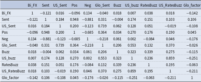

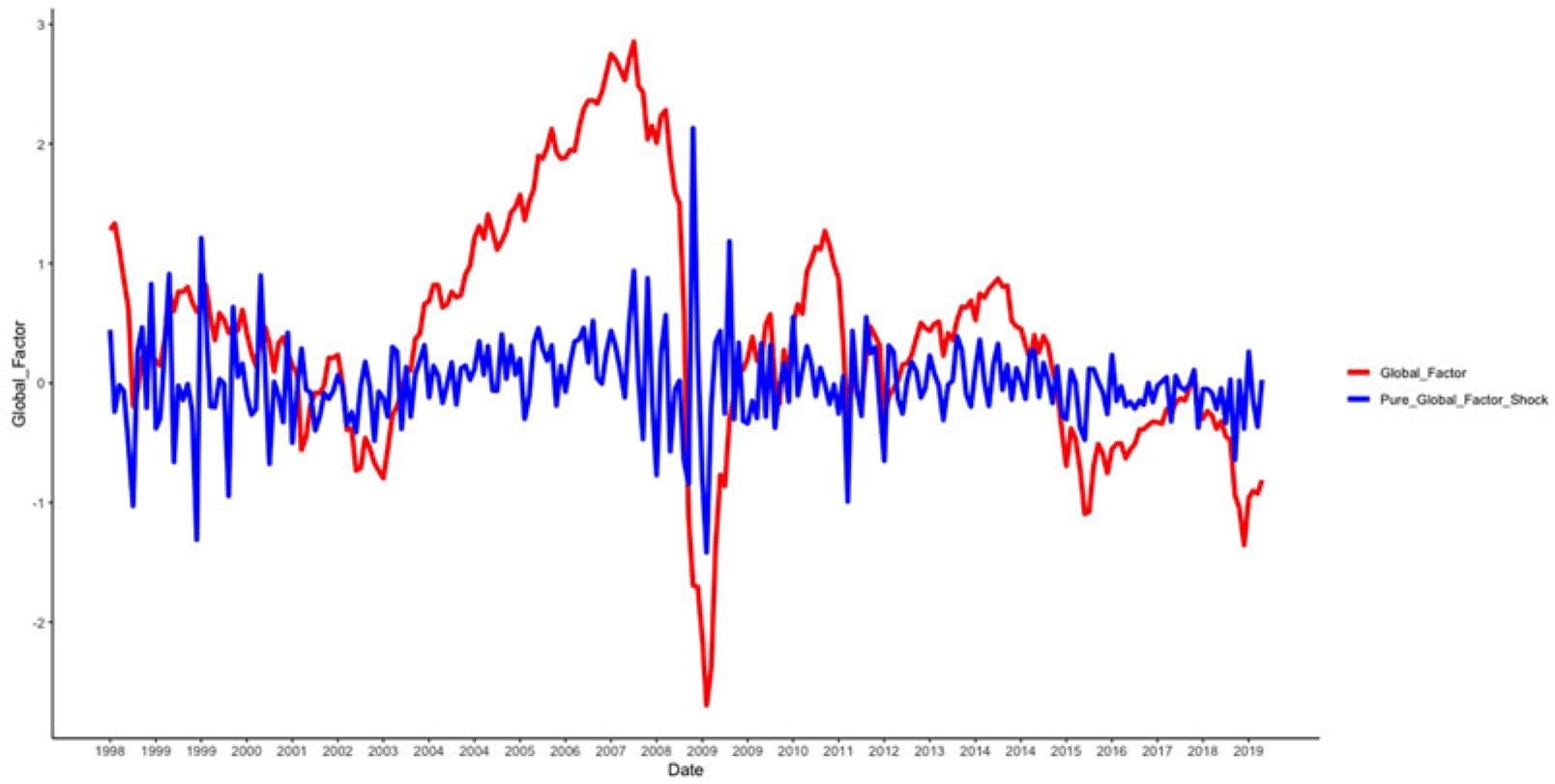


 Open access