


1. Introduction
End Devonian Mass Extinction (EDME) was a severe and distinct biotic crisis affecting terrestrial and marine ecosystems in the latest Famennian Stage (Fig. 1). It was coincident with a short glacial episode within the range of Retispora lepidophyta – a cosmopolitan miospore of latest Famennian age (Maziane et al. Reference Maziane, Higgs and Streel1999; Caputo et al. Reference Caputo, Melo, Streel, Isbell, Fielding, Frank and Isbell2008; Isaacson et al. Reference Isaacson, Díaz-Martínez, Grader, Kaldova, Bábek and Devuyst2008; Lakin et al. Reference Lakin, Marshall, Troth, Harding, Becker, Königshof and Brett2016). Proven glacigenic deposits are described in central South America (Díaz-Martínez & Isaacson, Reference Díaz-Martínez, Isaacson, Embry, Beauchamp and Glass1994; Cunha et al. Reference Cunha, Melo and Silva2007; Vaz et al. Reference Vaz, Mata Rezende, Filho and Travassos2007; Wicander et al. Reference Wicander, Clayton, Marshall, Troth and Racey2011; Caputo & Dos Santos, Reference Caputo and Dos Santos2019) and the Appalachian Basin of North America (Brezinski et al. Reference Brezinski, Cecil, Skema and Stamm2008, Reference Brezinski, Blaine-Cecil and Skema2010). These indicate a near-polar ice centre in western Gondwana and a temperate ice centre in the southern margin of Euramerica respectively (Fig. 2).
Chronostratigraphy of the latest Famennian (Devonian) and Tournaisian (Mississippian) Stages. Standard conodont schemes from Aretz et al. (Reference Aretz, Herbig, Wang, Gradstein, Ogg, Schmitz and Ogg2016) and Becker et al. (Reference Becker, Marshall, Da Silva, Gradstein, Ogg, Schmitz and Ogg2020). Standard Western European miospore biostratigraphic schemes and occurrences from Streel et al. (Reference Streel, Higgs, Loboziak, Riegal and Steemans1987) and Maziane et al. (Reference Maziane, Higgs and Streel1999). Those from South America are from Melo & Playford (Reference Melo and Playford2012) and Playford & Melo (Reference Playford and Melo2012) with gaps in the type sections indicated by crosses. EDME crisis intervals are from Becker et al. (Reference Becker, Kaiser, Aretz, Becker, Königshof and Brett2016). Rhenish Massif Standard Succession from Becker et al. (Reference Becker, Kaiser, Aretz, Becker, Königshof and Brett2016) and Herbig et al. (Reference Herbig, Korn, Amler, Hartenfels and Jäger2019). DS = Drewer Sandstone, HBS = Hangenberg Black Shale, HSh = Hangenberg Shale, HSst = Hangenberg Sandstone, Lst = Limestone. Proven glacial deposits are found within the range of R. lepidophyta, mostly LE/LN, and the mid-Tournaisian PC/PD zones (see Lakin et al. Reference Lakin, Marshall, Troth, Harding, Becker, Königshof and Brett2016).

Early Mississippian (350 Ma) palaeogeography, redrawn from Domeier & Torsvik (Reference Domeier and Torsvik2014). ‘S. Am’ and ‘N. Am’ are South America and North America, respectively. Latest Famennian ice centres are highlighted. Proven glacigenic deposits are found in: (1) Brazil (Cunha et al. Reference Cunha, Melo and Silva2007; Filho et al. Reference Filho, Eiras and Vaz2007; Milani et al., Reference Milani, Melo, Souza, Fernandez and Franca2007; Vaz et al. Reference Vaz, Mata Rezende, Filho and Travassos2007; Caputo et al. Reference Caputo, Melo, Streel, Isbell, Fielding, Frank and Isbell2008; Melo & Playford, Reference Melo and Playford2012); (2) Bolivia (Díaz-Martínez & Isaacson, Reference Díaz-Martínez, Isaacson, Embry, Beauchamp and Glass1994; Isaacson et al., Reference Isaacson, Palmer, Mamet, Cooke and Sanders1995; Wicander et al. Reference Wicander, Clayton, Marshall, Troth and Racey2011); and (3) Appalachia (Ettensohn et al., Reference Ettensohn, Lierman and Mason2009; Brezinski et al. Reference Brezinski, Blaine-Cecil and Skema2010). Putative ice centres are documented in (4) Africa by Theron Reference Theron(1993), Evans (Reference Evans1999), Streel & Theron (Reference Streel and Theron1999), Klett Reference Klett(2000), Streel et al. (Reference Streel, Caputo, Loboziak, Melo and Thorez2000), Almond et al. (Reference Almond, Marshall and Evans2002) and Isaacson et al. (Reference Isaacson, Díaz-Martínez, Grader, Kaldova, Bábek and Devuyst2008).

EDME is also known as the Hangenberg Crisis in the Rhenish Massif standard succession. It was of 100–300 ka duration and has been divided into three main intervals (Kaiser et al. Reference Kaiser, Aretz, Becker, Becker, Königshof and Brett2016). The lower crisis interval (or Hangenberg Black Shale event – HBS) is associated with high-total-organic-carbon (TOC) black shales, positive carbon isotope excursions (PCIEs), and widespread marine anoxia, e.g. in Europe (Brand et al. Reference Brand, Legrand-Blain and Streel2004; Buggisch & Joachimski, Reference Buggisch and Joachimski2006; Kaiser et al. Reference Kaiser, Becker, Hartenfels, Aboussalem, Becker, El Hassani and Abdelfatah2013; Kumpan et al. Reference Kumpan, Bábek, Kalvoda, Frýda and Grygar2013, Reference Kumpan, Bábek, Kalvoda, Grygar and Frýda2014), China (Qie et al. Reference Qie, Liu, Chen, Wang, Mii, Zhang, Huang, Yao, Algeo and Luo2015), Vietnam (Komatsu et al. Reference Komatsu, Kato, Hirata, Takashima, Ogata, Oba, Naruse, Ta, Nguyen, Dang, Doan, Nguyen, Sakata, Kaiho and Konigshof2014), Tibet (Liu et al. Reference Liu, Kerp, Peng and Zhu2019) and North America (Saltzman, Reference Saltzman2005; Cramer et al. Reference Cramer, Saltzman, Day, Witzke, Pratt and Holmden2008; Myrow et al. Reference Myrow, Strauss, Creveling, Sicard, Ripperdan, Sandberg and Hartenfels2011, Reference Myrow, Hanson, Phelps, Creveling, Strauss, Fike and Ripperdan2013; Over, Reference Over2020). The HBS is commonly interpreted as transgression, but it also contains regressive proxies and so could more likely represent increased terrigenous input onto carbonate shelves (Kaiser et al. Reference Kaiser, Becker, Steuber and Aboussalem2011; Bábek et al. Reference Bábek, Kumpan, Kalvoda and Grygar2016). Extinction primarily affected marine organisms, such as ammonoids, trilobites and conodonts (Becker, Reference Becker1992; Chlupac et al. Reference Chlupáč, Feist and Morzadec2000; Corradini et al. Reference Corradini, Spalletti, Kaiser, Matyja, Albanesi and Ortega2013; Kaiser et al. Reference Kaiser, Aretz, Becker, Becker, Königshof and Brett2016). Recent reinvestigations of European and Vietnamese sections show a more complicated picture. Firstly, anoxic conditions sometimes persist into the lower Tournaisian (Paschall et al. Reference Paschall, Carmichael, Königshof, Waters, Ta, Komatsu and Dombrowski2019). And secondly, corresponding negative carbon isotope excursions (NCIEs) are recognized preceding the HBS in the upper praesulcata zone / lower costatus–kockeli interregnum zone and Devonian/Carboniferous Boundary (DCB) (Matyja et al. Reference Matyja, Woroncowa-Marcinowska, Filipiak, Brański and Sobień2020; Pisarzowska & Racki, Reference Pisarzowska, Racki and Montenari2020; Pisarzowska et al. Reference Pisarzowska, Rakociński, Marynowski, Szczerba, Thoby, Paszkowski, Perri, Spalletta, Schönlaub, Kowalik and Gereke2020).
The middle crisis interval is characterized by eustatic sea-level fall and deposition of the ‘Hangenberg Sandstone’ and equivalents (van Steenwinkel, Reference Van Steenwinkel1993). Eustatic sea-level fall immediately below the DCB is supported by regressive facies and/or detrital indicators observed from diverse geological settings (see Kaiser et al. Reference Kaiser, Steuber and Becker2008; Weber et al. Reference Weber, Francis, Harris and Clarke2008; Kumpan et al. Reference Kumpan, Bábek, Kalvoda, Frýda and Grygar2013, Reference Kumpan, Bábek, Kalvoda, Grygar and Frýda2014; Bábek et al. Reference Bábek, Kumpan, Kalvoda and Grygar2016; Carmichael et al. Reference Carmichael, Waters, Batchelor, Coleman, Suttner, Kido, Moore and Chadimová2016). Kaiser et al. (Reference Kaiser, Becker, Steuber and Aboussalem2011) estimated c. 100 m of relative sea-level fall in Morocco, which is comparable to the <100 m of marine incision observed in central Europe and North America (van Steenwinkel, Reference Van Steenwinkel1993; Brezinski et al. Reference Brezinski, Blaine-Cecil and Skema2010).
The upper crisis interval at the DCB is associated with eustatic sea-level rise and severely affected terrestrial plants/miospores, tetrapods and fish (Streel & Marshall, Reference Streel, Marshall and Wong2006; Sallan & Coates, Reference Sallan and Coates2010; Marshall, Reference Marshall2020).
Several factors have been proposed as causes of EDME, ranging from meteorite impacts, marine anoxia, global carbon cycle change, palaeoclimate and sea-level change, to magmatic activity (Kaiser et al. Reference Kaiser, Aretz, Becker, Becker, Königshof and Brett2016; Pisarzowska et al. Reference Pisarzowska, Rakociński, Marynowski, Szczerba, Thoby, Paszkowski, Perri, Spalletta, Schönlaub, Kowalik and Gereke2020).
There are relatively few studies on the nature of the DCB in the glaciated southern palaeolatitudes of western Gondwana, likely because key fossil groups are extremely rare or absent. Palynostratigraphy can tie Late Devonian global schemes and events into South America (e.g. Troth et al. Reference Troth, Marshall, Racey and Becker2011; Melo & Playford, Reference Melo and Playford2012), which allows for a reinvestigation of the DCB from a siliciclastic high-palaeolatitude area affected by glaciation. Our objectives are to: (1) revisit and describe a diamictite sequence from western Gondwana (Bolivian Altiplano); (2) interpret the palynological record; and (3) test whether positive isotope excursions in organic carbon can be recognized. These results can then be compared against the global record to inform debates regarding EDME and global environmental change at the DCB.
2. Study area
The Altiplano is a high-altitude plateau formed during Andean orogenic uplift, which segmented the Palaeozoic stratigraphy into NW–SE-orientated tectonic zones (Fig. 3a; Sempere, Reference Sempere, Tankard, Suarez and Welsink1995; Gregory-Wodzicki, Reference Gregory-Wodzicki2000; Capitano et al., Reference Capitano, Faccenna, Zlotnik and Stegman2011; Barnes et al. Reference Barnes, Ehler, Insei, McQuarrie and Poulson2012). Latest Famennian glacial diamictites (dropstone-in-shales) are reported in the Cumaná Formation, which crops out for c. 80 km from the Isla del Sol to the Copacabana and Cumaná Peninsulas (Fig. 3b; Díaz-Martínez & Isaacson, Reference Díaz-Martínez, Isaacson, Embry, Beauchamp and Glass1994; Díaz-Martínez et al. Reference Díaz-Martínez, Vavrdová, Bek and Isaacson1999).
Location maps. (a) Bolivia. (b) Lake Titicaca area. (c) Chaguaya study area with log locations and geological map overlain. (d) Bolivian Altiplano lithostratigraphy modified from Díaz-Martínez (Reference Díaz-Martínez1996) and Grader et al. (Reference Grader, Díaz-Martínez, Davydov, Montanez, Tair, Isaacson, Díaz-Martínez and Rabano2007). Dark triangles in (d) indicate the units are diamictite-bearing.

The study area is on the NE shore of Lake Titicaca, near the community of Chaguaya (Fig. 3b–c). There is an uninterrupted Devonian–Mississippian sequence that contains diamictites, the global index miospore Retispora lepidophyta and claystones suitable for palynological recovery (Díaz-Martínez, Reference Díaz-Martínez1992; Díaz-Martínez et al. Reference Díaz-Martínez, Vavrdová, Bek and Isaacson1999; Vavrdová & Isaacson, Reference Vavrdová and Isaacson1999; di Pasquo et al. Reference Di Pasquo, Grader, Isaacson, Souza, Iannuzzi and Díaz-Martínez2015 di Pasquo et al. Reference Di Pasquo, Grader, Isaacson, Souza, Iannuzzi and Díaz-Martínez2015 di Pasquo et al. Reference Di Pasquo, Grader, Isaacson, Souza, Iannuzzi and Díaz-Martínez2015). These make it an ideal study area.
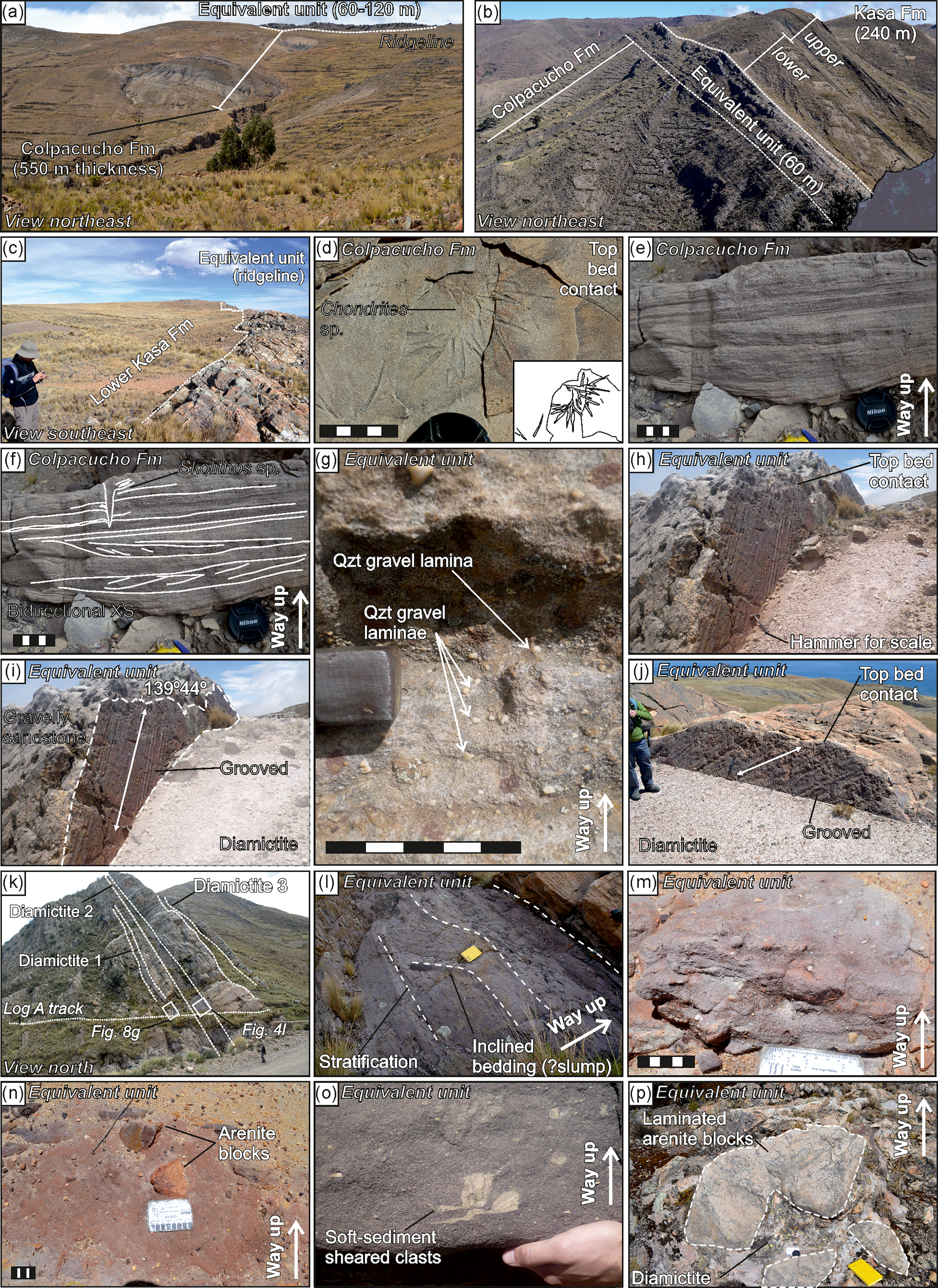
Seventeen stratigraphic logs are presented. Log A is a road section called ‘Villa Molino’ and Logs B–Q were measured along an approximately strike-parallel, 7 km long topographic ridgeline (Fig. 3c). The stratigraphy is mapped from field observations, log sections and satellite imagery and compared to the regional lithostratigraphy of Díaz-Martínez (Reference Díaz-Martínez1996) and Grader et al. (Reference Grader, Díaz-Martínez, Davydov, Montanez, Tair, Isaacson, Díaz-Martínez and Rabano2007) (Fig. 3c–d). The Cumaná and Siripaci Formations are not present. An equivalent unit to the Cumaná Formation has been identified (‘Cumana Formation equivalent unit’: CFEU); it is distinct, well exposed and crops out along the ridgeline (Fig. 4a–b). The CFEU is an informal classification termed by this study. It is defined by its two distinct bounding surfaces: a lower erosive contact with apparent down-cut and an upper conformable contact into not well-exposed claystones. It can be correlated to the Cumaná Formation based on the presence of key palynological taxa (i.e. Retispora lepidophyta and Umbellisphaeridium saharicum). The top of the CFEU is used as a tie-point between log sections (Fig. 4c). The Siripaci Formation is presumed absent under the intra-Carboniferous unconformity (Fig. 3d).
Field photographs. (a) Ridgeline. (b) View of the area north of Log A, photo taken at base Log B. (c) View to southeast, photo taken at base Log E. (d) Bioturbation in the Colpacucho Formation at Log A interpreted as Chondrites sp. See inset for overlay of bioturbation. (e) Colpacucho Formation sandstones at Log A. (f) Bidirectional cross-stratification and Skolithos sp. bioturbation overlain at Log A. (g) Gravelly sandstones in the Cumana Formation Equivalent Unit in Log N with quartz gravel laminae. (h) Strongly cemented gravel bed at Log N. (i) Strongly cemented gravel bed at Log N with details on grooves annotated. (j) Strongly cemented gravel bed, weathered. (k) Log A location with the three diamictite beds annotated. Note the lateral continuity of these beds. Location of (l) and Figure 8g overlain. (l) Inclined and parallel stratification in diamictite facies at Log A. (m) Diamictite with quartz gravel clasts at Log P. (n) Arenite sandstone blocks in diamictite at Log P. (o) Diamictite with soft-sediment sheared clasts at Log A. (p) Metre-scale laminated arenite sandstone blocks at Log I. Scale bar is 5 cm. Field notebook is 13 × 20 cm.
3. Materials, methods and terminology
Sedimentary logs were measured in the field at 1:50 scale using a tape measure and with the aid of a Jacob’s Staff and Abney level. The term ‘diamictite’ is used as a descriptive term that classifies poorly sorted sedimentary rocks with varied grain and clast sizes from clay to boulders (Flint et al. Reference Flint, Sanders and Rodgers1960a, Reference Flint, Sanders and Rodgers1960b). The Moncrieff (Reference Moncrieff1989) classification system is used to discriminate diamictites from other poorly sorted rocks. The classification of Evans et al. (Reference Evans, Phillips, Hiemstra and Auton2006) was used to interpret diamictite facies.
Whole-rock claystone samples were collected from outcrop at a shallow depth (<20 cm). All palynological processing was by standard methods (see Phipps & Playford, Reference Phipps and Playford1984), including HCl (37 %) and HF (60 %) followed by decant washing to neutral and sieving at 15 μm. This was followed by a brief short treatment in hot HCl (37 %) to remove neoformed fluorides. The samples were then rapidly diluted into ˜200 ml of water and re-sieved before storing in a vial. Whole kerogen samples were not sieved at 15 μm and directly strewn after HF digestion.
Miospore schemes and index taxa discussed are from western Europe (see Clayton et al. Reference Clayton, Coquel, Doubinger, Gueinn, Loboziak, Owens and Streel1977; Streel et al. Reference Streel, Higgs, Loboziak, Riegal and Steemans1987; Higgs et al. Reference Higgs, Clayton and Keegan1988; Maziane et al. Reference Maziane, Higgs and Streel1999) and the Amazon Basin, Brazil (see Loboziak et al. Reference Loboziak, Caputo and Owens1986, Reference Loboziak, Melo, Playford and Streel1999, Reference Loboziak, Caputo and Melo2000, Reference Loboziak, Melo, Streel and Koutsoukos2005; Melo & Loboziak Reference Melo and Loboziak2000, Reference Melo and Loboziak2003; Loboziak & Melo, Reference Loboziak and Melo2002; Playford & Melo, Reference Playford and Melo2009, Reference Playford and Melo2012; Melo & Playford, Reference Melo and Playford2012). Biozones are defined on the first occurrences (FOs) of key miospore taxa (Fig. 1). The term ‘phytoplankton’ refers to the preserved cysts of acritarchs and prasinophytes. Particulate organic matter (POM) includes spore, phytoplankton and phytoclasts (i.e. plant debris) that exist as particulate fragments. Amorphous organic matter (AOM) is structureless under light microscopy and is likely formed in the water column and/or sedimentary substrate via microbial activity (Pacton et al. Reference Pacton, Gorin and Vasconcelos2011).
Palynological investigation was difficult due to a high degree of degradation typical of the area (see also Díaz-Martinez et al. Reference Díaz-Martínez, Vavrdová, Bek and Isaacson1999). Only the samples showing the best-preserved palynomorphs were counted to at least 200 specimens for statistical data, with all other samples used for presence/absence data only. Nevertheless, c. 75 % of counted specimens could not be identified to a species/generic level or even in open nomenclature. This has likely reduced the total taxon count and imparted a significant preservation bias as: (1) robust forms are likely to have preserved more than fragile ones, and (2) taxa with distinctive features are more readily identified over those with subtle defining characteristics easily obscured by degradation. As mitigation, certain specimens were grouped into larger categories for the relative abundances, such as genera (e.g. Umbellasphaeridium spp.) or sculpture characteristics (e.g. apiculate spores).
The carbon content in the samples for the TOC profiles was measured using a Carlo-Erba EA-1108 elemental analyser. Between 2 and 3 mg of both decarbonated and original sample were separately analysed with the machine calibrated using a low Total Carbon (TC) ‘soil’ standard (1.55 %). Between every 10 samples a check was made using the standard as an unknown.
Organic carbon isotope analysis was undertaken by Iso-Analytical Ltd. They employed an Elemental Analyser – Isotope Ratio Mass Spectrometry (EA-IRMS) technique using a Europa Isotope Ratio Mass Spectrometer. Measurements were calibrated to a wheat flour standard (δ13CV-PDB −26.43 ‰) and cross-checked during experimental runs against beet sugar (δ13CV-PDB −26.03 ‰) and cane sugar (δ13CV-PDB −11.64 ‰) standards. All are calibrated against the international standard IAEA-CH-6 (sucrose, δ13CV-PDB −10.43 ‰).
4. Results
4.a. Stratigraphy
4.a.1. Colpacucho Formation
The Colpacucho Formation is at least 560 m thick in Log I, but its basal contact was not observed (Figs 5a and 6). It is composed of claystones that contain siderite concretions and subordinate interbedded sandstones. Larger sandstone interbeds can reach up to 1 m thick, and are cross-bedded, laminated and/or massive with occasional channels. Where preserved (Log A), its uppermost 100 m coarsens upwards into massive, laminated, cross-stratified and/or variably bioturbated sandstones. Bioturbation consists of Chondrites sp. with rare Skolithos sp. (Fig. 4d–f). The uppermost Colpacucho Formation is defined at the point at which the unit transitions from claystone- to sandstone-dominated. Where the sediment has been significantly bioturbated, there is a mottled texture. At 124–141 m height in Log A, the cross-stratified sandstones contain rare claystone rip-up clasts, gravel laminae and bidirectional cross-stratification (Fig. 4f).
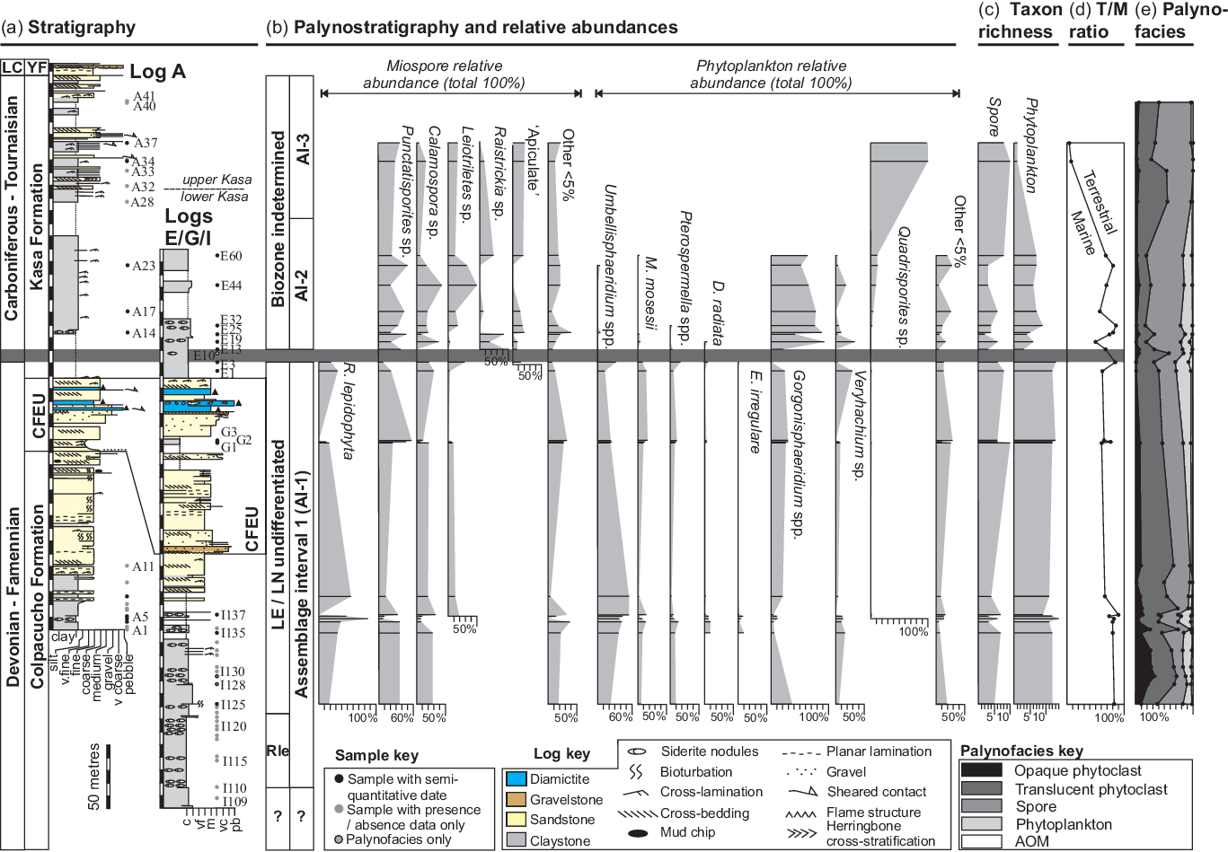
Composite stratigraphy and palynostratigraphy. Horizontal dark bar is Devonian–Carboniferous boundary interval. (a) Stratigraphy. Columns from left to right are age and formation/unit. White gaps in the logs are gaps in exposure where no log was taken. LC = Late Carboniferous, YF = Yaurichambi Formation, ‘CFEU’ refers to Cumaná Formation Equivalent Unit. (b) Palynostratigraphy and relative abundances. Columns from left to right are biozones and assemblage intervals (AIs). (c) Taxonomic richness, i.e. number of spore and phytoplankton taxa present. (d) Terrestrial/marine ratio of counted specimens. (e) Palynofacies.

4.a.2. ‘Cumaná Formation equivalent unit’ (CFEU)
The CFEU varies in thickness from 58 m at Log A to 140 m at Log I. Overall, it is composed of coarse sandstones, gravel and diamictites. Its basal contact is a single or occasionally stacked gravelstone and/or breccia-conglomerate overlying an erosional surface. Variable incision of c. 100 m into the underlying bioturbated sandstones of the Colpacucho Formation is inferred from the correlation of sections (Fig. 6a–b). This basal surface marks a subtle yet defining change in sedimentary character, above which sandstones are more thickly bedded, coarser and non-bioturbated. The unit can be broadly split into: (1) a lower sandstone-dominated sub-unit; (2) a laterally and vertically discontinuous, poorly exposed interbedded sub-unit; and (3) an upper sub-unit of cross-laminated sandstones and diamictites (Fig. 6a).
The lower sub-unit is predominantly composed of two facies. The first comprises thickly bedded, cross-stratified and well-sorted medium to coarse grained sandstones. The second comprises matrix-supported and poorly sorted gravelly sandstones that contain gravel and conglomeratic laminae that occasionally overlie erosive scours (Fig. 4g). These facies broadly coarsen upwards.
The interbedded sub-unit consists of cross-laminated sandstones, claystones and laterally restricted poorly sorted purple siltstones and muddy sandstones. The latter are very similar to diamictite facies but lack the coarser sediment fraction and clasts. Hummocky and swaley cross-lamination was observed at 70 m in section Log H. It fines upwards into poorly exposed claystones in Log G (Fig. 6a).
The boundary between the lower and upper sub-units is typically marked by strongly cemented gravel beds that can be correlated between sections (Figs 4h–j and 6a). They have a common stratigraphic association along the ridgeline; they are exclusively found on the top surface of coarsening-upwards gravelly sandstone facies and are always overlain by diamictite (Fig. 7). They are poorly sorted, 5–20 cm thick and contain interspersed quartz gravel that is especially concentrated on the top surface. The top surfaces have a patchy, weathered exposure, and commonly host linear striations and grooves <1 cm deep (Fig. 4h–j).
Stratigraphic association of the strongly cemented gravel beds at (a) Log I and (b) Log N. These logs are laterally separated by 1200 m.

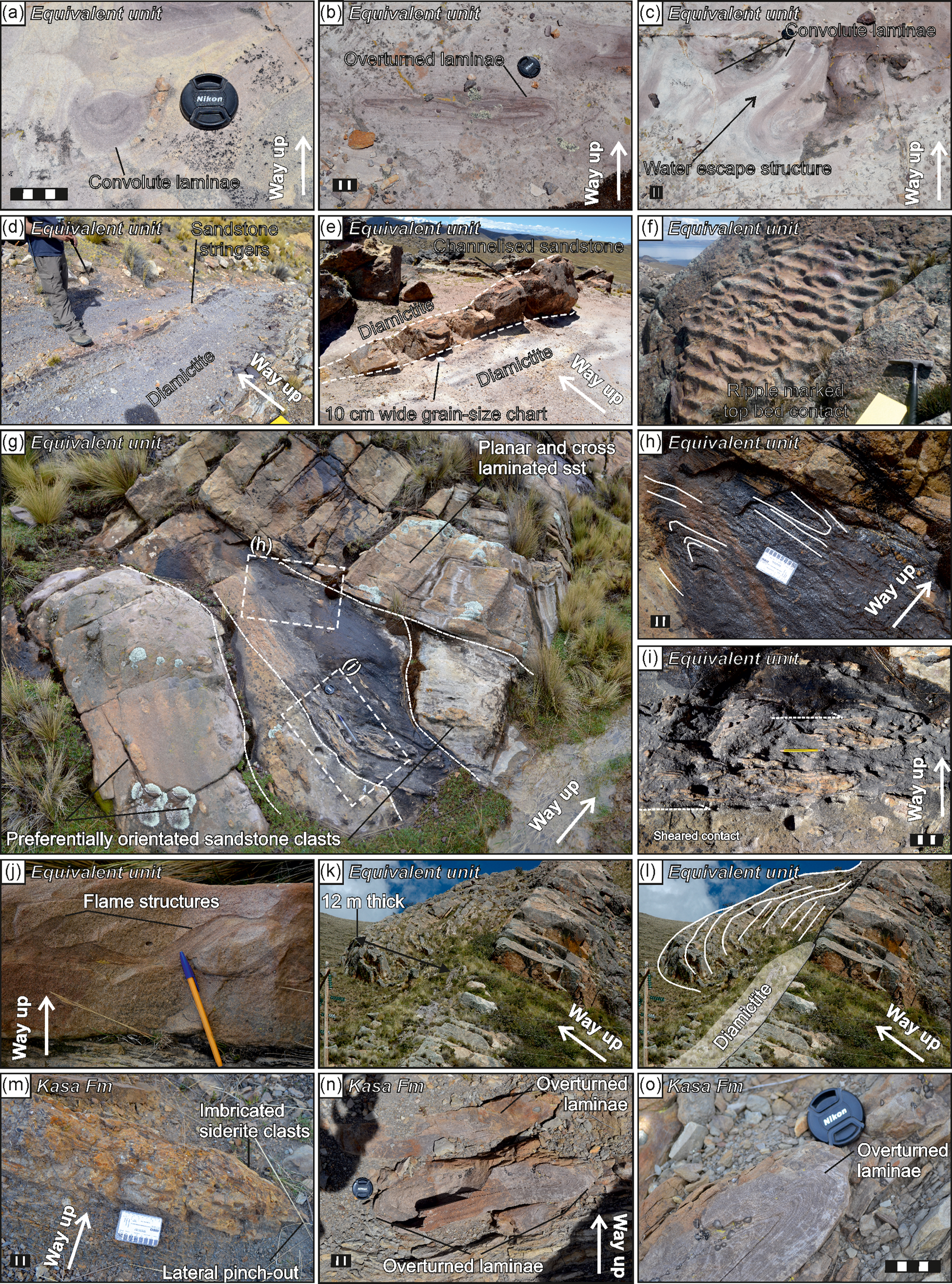
The upper sub-unit is predominantly composed of diamictites and sandstone facies (Fig. 6a). The diamictites are ≤10 m thick, stratified and matrix-supported clast-rich to clast-poor sandy diamictites. They have relatively straight contacts that are rarely sheared and mostly conformable (Fig. 4k). Exposure is recessive and tends to be obscured by modern soil profiles. Stratification is subtle, defined by colour banding, rare lamination and faint bedding, which can be non-planar (Fig. 4l). The matrix is micaceous, poorly sorted (from clay to gravel) and weathers a distinctive purple colour (Fig. 4m). Clasts are composed of quartz gravel/pebbles (randomly orientated) and arenite sandstone lithics (Fig. 4m–n). A rare number of clasts show soft-sediment shearing (Fig. 4o). Clast size and content is highly variable and diamictites are in compositional continuity with muddy sandstones where clasts are absent (Fig. 6a). Larger sandstone lithic blocks up to 1 m in diameter were observed in Log I (Fig. 4p). Overturned and convolute laminae are common (Fig. 8a–c). Cross-stratified sandstones are commonly interbedded with the diamictites; either as discrete stringers (<2 cm thick) or as metre-scale beds (Fig. 8d–e). The sandstone facies become progressively more thickly bedded and ripple-marked with height (Figs 7 and 8f). Sheared contacts and convoluted and/or overturned stratification, including flame structures, were observed across the ridgeline but especially at Log A (Fig. 8g–j). Immediately to the southeast of Log A there is a 22 m thick overturned sandstone that lies above the topmost diamictite bed and contained diamictite intraclasts (Fig. 8k–l).
Field photographs. (a) Convolute laminae in diamictite at Log F. (b) Overturned laminae in diamictite at Log F. (c) Convolute laminae and possible water-escape structures in diamictite at Log F. (d) Interbedded thin sandstones in diamictite. (e) Sandstone channel in diamictite at Log P. (f) Ripple-marked sandstone at near top CFEU. (g) Sheared sandstones in CFEU at Log A. Locations of (h–i) overlain. (h) Overturned laminae in sandstones. See (g) for location. (i) Soft-sediment deformation and sheared basal contact. See (g) for location. (j) Flame structure in CFEU sandstones at Log A. (k) Slump structure at top CFEU at Log A. (l) Slump structure annotated showing position above a diamictite décollement. (m) Laterally restricted debris flow with imbricated siderite clasts in the Kasa Formation at Log A. (n) Overturned laminae in forming a sheaf fold in the Kasa Formation at Log A. (o) Closer photo of overturned laminae in (n). Scale bar is 5 cm.
4.a.3. Kasa Formation
The Kasa Formation has a measured thickness of 240 m at Log A. The basal contact is conformable and laterally correlatable. The Kasa Formation is divided into a lower claystone-dominated unit and an upper interbedded unit (Fig. 5a).
The lower unit is c. 150 m thick. It is composed of claystones that contain siderite concretionary horizons and interbedded cross-laminated sandstones.
The upper unit is c. 90 m thick. Sandstones are cross-stratified, finely interbedded and with rare bioturbation on exposed bed surfaces. There are several thinly interbedded matrix-supported and clast-supported diamictite and conglomerate beds (<1m thick) that overlie sharp erosive contacts (Fig. 8m). Associated with these are sandstones with overturned laminae and sheaf folds (Fig. 8n–o). The diamictite and conglomerate beds are typically lensoid with limited lateral extent. There is a preferred orientation in the clasts along a sub-horizontal fabric (Fig. 8m – ‘Imbricated siderite clasts’). Clasts are well-rounded and primarily composed of siderite nodules and rarer quartz pebbles.
4.b. Palynology
Three palynological assemblage intervals (AIs) are identified. Changes in the miospore and phytoplankton fractions occur at the same stratigraphic levels and are discussed together. See Figures 9 and 10 for palynological plates of the taxa discussed, Table 1 for total assemblage abundances, and the Supplementary Material (available online at https://doi.org/10.1017/S0016756821000741) for the presence/absence data.
Palynological plate 1: miospores. Scale bars are 20 μm and 50 μm. (a) Anapiculatisporites ampullaceus. (b) Anapiculatisporites semicuspidatus. (c) Apiculatisporites quadrosii. (d) Apiculiretusispora sp. (e) Auroraspora sp. (f) Calamospora sp. (g) Claytonispora sp. (h) Convolutispora major. (i) Cymbosporites sp. (j) Densosporites annulatus. (k) Emphanisporites rotatus. (l) Endosporites angustus. (m) Grandispora protea. (n) Indotriradites dolianitii morphon. (o) Indotriradites explanatus. (p) Indotriradites explanatus. (q) Indotriradites viriosus. (r) Knoxisporites literatus. (s) Knoxisporites literatus. (t) Leiotriletes sp. (u) Neoraistrickia sp. (v) Punctatisportites spp. (w) Raistrickia sp. (x) Raistrickia sp. (y) Retispora lepidophyta. (z) Retusotriletes incohatus. (aa) Vallatisporites sp. (ab) Verrucosisporites congestus. (ac) Verrucosisporites depressus. (ad) Verrucosisporites nitidus. (ae) Waltzispora lanzonii. (af) Waltzispora lanzonii aberrant. (ag) Waltzispora lanzonii aberrant. (ah) Waltzispora sp. 1. (ai) Aratrisporites saharaensis.

Palynological plate 2: Acritarchs and prasinophytes. (a) Cymatiosphaera ambotrocha. (b) Duvernaysphaera radiata. (c) Maranhites mosesii. (d) Maranhites mosesii. (e) Petrovina connata. (f) Pterospermella spp. (P. pernambucensis). (g) Quadrisporites sp. (h) Quadrisporites sp. (i) Chomotriletes vedugensis. (j) Evittia sommeri. (k) Exochoderma irregulare. (l) Gorgonisphaeridium spp. (m) Gorgonisphaeridium spp. (n) Gorgonisphaeridium spp. (o) Gorgonisphaeridium winslowiae. (p) Horologinella quadrispina. (q) Micrhystridium breve group. (r) Micrhystridium pentagonale group. (s) Multiplicisphaeridium ramusculosum. (t) Pyloferites pentagonale. (u) Schizocystia bicornuta. (v) Stellinium comptum. (w) Stellinium micropolygonale. (x) Stellinium sp. 1. (y) Umbellasphaeridium deflandrei. (z) Umbellasphaeridium saharicum. (aa) Umbellasphaeridium saharicum. (ab) Veryhachium lairdii group. (ac) Veryhachium trispinosum group. (ad) Incertae sedis 1. (ae) Incertae sedis 2. (af) Incertae sedis 2. (ag) Leiosphere sp. (ah) Leiosphere sp. (ai) Lophosphaeridium sp.

Total relative abundance by all samples in each assemblage interval.

4.b.1. Assemblage interval 1: Retispora lepidophyta / Umbellasphaeridium spp
AI-1 is defined as the range of Retispora lepidophyta in the counted samples from sample ‘I110’ in the Colpacucho Formation to ‘E3’ in the lowermost Kasa Formation (Fig. 5a–b).
The miospore fraction is relatively poorly preserved, difficult to fully speciate and of low diversity. It is characterized by the high relative abundance of R. lepidophyta, which comprises up to a third of the total miospore count. Morphologically simple, single-walled and non-apiculate miospore taxa are common (Punctatisporites sp., Calamospora sp. and Leiotriletes sp.) and comprise half of the total miospore fraction (Fig. 5b).
Age-diagnostic miospore taxa are rare and were observed in out-of-count presence/absence data only. However, AI-1 does contain the First Occurrences (FOs) of key taxa, such as Knoxisporites literatus, Indotriradites explanatus and Verrucosisporites nitidus (Fig. 5b). Long-lived Devonian and Early Carboniferous species, such as Densosporites annulatus, Emphanisporites rotatus and Retusotriletes incohatus, were also identified.
The phytoplankton fraction has relatively high taxonomic richness and is characterized by the high relative abundance of Umbellasphaeridium saharicum and to a lesser extent Umbellasphaeridium deflandrei and indeterminate (degraded) Umbellasphaeridium sp. (Fig. 5b – ‘Umbellasphaeridium spp.’). There are also common Gorgonisphaeridium spp., Maranhites mosesii, Veryhachium trispinosum group, Veryhachium lairdii group, Pterospermella spp., Duvernaysphaera radiata and Exochoderma irregulare. Rare taxa include Pyloferites pentagonale, Stellinium micropolygonale and Schizocystia bicornuta
4.b.2. Assemblage interval 2: Gorgonisphaeridium spp. dominated
The base of AI-2 is defined at the last occurrence (LO) of R. lepidophyta in sample ‘E3’ and is accompanied by an increase in Gorgonisphaeridium spp. abundance between samples ‘E13’ and ‘E19’ (Fig. 5a–b). The base of AI-2 is also associated with significant reductions in spore and phytoplankton taxonomic richness (Fig. 5c). The interval is entirely constrained within the lower unit of the Kasa Formation (Fig. 5b).
The miospore fraction is dominated by the morphologically simple, single-walled and non-apiculate Punctatisporites sp., Calamospora sp. and Leiotriletes sp. genera, which comprise >60 % of the total miospore count. There is a relative increase in single-walled apiculate miospores: Anapiculatisporites sp., Apiculatisporites sp., Apiculiretusispora sp. (Fig. 5b – ‘apiculate’) and Raistrickia sp. (Fig. 5b – ‘Raistrickia’).
Age-diagnostic miospore taxa are extremely rare, and difficult to speciate with confidence. Only a single age-diagnostic species, Anapiculatisporites semicuspidatus, had its FO within AI-2.
The phytoplankton fraction is relatively impoverished compared to AI-1 and characterized by the high relative abundance of Gorgonisphaeridium spp., which accounts for 73 % of total identified phytoplankton. AI-2 is also associated with the long-lived Palaeozoic to Mesozoic phytoplankton genera Veryhachium spp., Micrhystridium spp. and Quadrisporites sp. These are minor components of AI-2, but their relative abundances are relatively unchanged from the preceding AI-1 (Fig. 5b). Those taxa which disappear entirely into AI-2 include E. irregulare, Gorgonisphaeridium winslowiae, Schizocystia bicornuta, Stellinium comptum and Stellinium sp. The following taxa persist into AI-2, but in extremely reduced numbers: D. radiata, Horologinella quadrispina, Lophosphaeridium sp., M. mosesii, Pterospermella spp., P. pentagonale, Stellinium micropolygonale, U. deflandrei and U. saharicum.
4.b.3. Assemblage interval 3: spore-dominated
The base of AI-3 is defined at the loss of the phytoplankton fraction (including Gorgonisphaeridium spp.) in sample ‘A34’ (Fig. 5b–d). It is spore- and phytoclast-dominated and ranges entirely within the upper Kasa Formation.
The miospore fraction is difficult to identify confidently due to poor preservation. However, Punctatisporites sp., Leiotriletes sp. and Calamospora sp. were common and comprise 49 % of the total miospore count. The rest are mostly single-walled apiculate genera such as Anapiculatisporites sp., Apiculatisporites sp., Apiculiretusispora spp., Claytonispora sp. and Raistrickia sp.
The following age-diagnostic miospore taxa had their FOs in AI-3 but are either extremely rare or limited to single occurrences. These are: Anapiculatisporites ampullaceus, Indotriradites dolianitii morphon, Indotriradites viriosus and Waltzispora lanzonii. Only a single specimen of W. lanzonii that conformed to its original type description was identified (see Daemon, Reference Daemon1974). Several unusual forms were observed with up to four poorly developed apical shoulders, which are comparable to those described by Playford & Melo (Reference Playford and Melo2010, Reference Playford and Melo2012). Waltzispora sp. 1 is morphologically like W. lanzonii but lacks shoulder apiculation. Additional age-diagnostic species have their FOs within AI-3 but are known from the Late Devonian. These include: Aratrisporites saharaensis, Convolutispora major, Verrucosisporites congestus and Verrucosisporites depressus (Playford & Melo, Reference Playford and Melo2012).
Phytoplankton are almost non-existent in AI-3. Only rare specimens of Quadrisporites sp. were observed in the counts. Specimens of other marine phytoplankton taxa were only sporadically observed in the presence/absence data.
4.b.4. Palynofacies
The palynofacies are dominated by terrestrially derived phytoclasts and spores, with only minor proportions of marine phytoplankton and amorphous organic matter (AOM) (Fig. 5e). Some broad trends are recognized. There is an upwards decrease in the relative abundance of the marine fraction (‘phytoplankton’ and ‘AOM’) in the uppermost Colpacucho Formation. The proportion of phytoclasts in the lower Kasa Formation (AI-2) is reduced. In contrast, there is a sudden increase in phytoclast content in the upper Kasa Formation (AI-3), coincident with the decrease in Terrestrial/Marine (T/M) ratio in the counts.
4.c. TOC and δ13Corganic
4.c.1. Colpacucho Formation
Total organic carbon values typically vary between 0.3 and 1.5 %, but peak at 2.5 % in sample A-10, which is coincident with an increase in phytoclast content (Fig. 11).
Geochemistry. Horizontal dark bar is DCB interval. (a) Stratigraphy – see Figure 5 for key. (b) Composite total organic carbon with three-point average curve. (c) Composite δ13Corganic with three-point average curve. (d) Expanded view of Logs D and E showing 2 ‰ PCIE in a continuous run of samples through the DCB.

Only those samples above the FO of Indotriradites explanatus (LE/LN zone) were processed for bulk δ13Corg as this is the level in which global PCIEs have been observed (Fig. 11; see also Kaiser et al. Reference Kaiser, Aretz, Becker, Becker, Königshof and Brett2016). δ13Corg values are variable within a c. 1 ‰ range (−24.3 to −25.16 ‰), with a mean average of −24.27 ‰.
4.c.2. Lower Kasa Formation
TOC averages 0.95 %. Trends appear negatively correlated with δ13Corg, but there is no overall statistical relationship (R 2 = 0.02).
There is a negative shift in bulk δ13Corg values of c. 2 ‰ compared to the uppermost Colpacucho Formation. There is an upwards positive trend throughout the lower Kasa Formation (samples D1 to A27) of 1.6 ‰. Within this trend there is at least one PCIE, and potentially two. These are more clearly observed in Logs D and E where there are near-continuous runs of samples at 1 m intervals (Fig 11f).
The lower 2 ‰ PCIE is at 13–22 m above the base lower Kasa Formation and is coincident with a negative TOC excursion of 0.8 %. Its base (sample E3) contains the last counted occurrence of Retispora lepidophyta. Particulate organic matter is noticeably darker and more degraded in samples through the 2 ‰ PCIE compared to those above and below (Fig. 12). Immediately above the PCIE, both TOC and bulk δ13Corg increase by c. 1 % and 1 ‰ respectively. This is accompanied by less degraded and more translucent POM and the lowest observation of AI-2 (Figs 5 and 12c).
Palynological assemblages in samples E1, E9 and E13 that were processed through standard techniques. Samples E1 and E13 are beneath and above the 2 ‰ PCIE respectively. Sample E9 is at the peak of the 2 ‰ excursion and shows much more degraded and darkened POM compared with those samples E1 and E13. Scale bars are 500 μm.

Processed palynological recovery was sparse through the 12–22 m interval in Log E (2 ‰ PCIE), despite the average TOC values of 0.52 %. This suggests that the bulk of the organic residue in the PCIE samples was in the <15 μm fraction lost during standard palynological processing (i.e. washed through the 15 μm nylon mesh). To investigate further, those palynological samples between 13 and 22 m height in Log E were reprocessed using HF only and with the <15 μm fraction retained. The resulting residues contained AOM and neoformed fluorides (the latter a consequence of HF reacting with clay minerals and trace calcium in the sample). This means that AOM was preferentially lost during palynological processing.
The second PCIE (1 ‰) is at 68–72 m in Log E and is accompanied by a negative TOC excursion of 0.7 %. However, due to the break in section at 47–68 m height it is only partially sampled (Fig. 11).
4.c.3. Upper Kasa Formation
TOCs and bulk δ13Corg increase markedly into the upper Kasa Formation to a maximum of 2.2 % and −23.9 ‰ respectively. This correlates with the total loss of the marine fraction and the increase in phytoclast content observed in AI-3 (Fig. 11). In the upper part, TOCs decrease to an average of 0.6 %.
5. Interpretation
5.a. Depositional history
5.a.1. Colpacucho Formation: open-marine
The Colpacucho Formation is an open-marine shelf environment based on the phytoplankton population observed in AI-1 and previous work (Díaz-Martínez, Reference Díaz-Martínez1991). The claystone-dominated lower part is interpreted as offshore. The uppermost Colpacucho is interpreted as a prograding shoreface (Fig. 13a). The high degree of bioturbation in the shoreface sands suggests environmental conditions were either more favourable for biological life or allowed for greater preservation potential. An absence of body fossils, spreite and back-fill structures suggests that bioturbation was caused by soft-bodied organisms, such as annelid or nematode worms. Tidal processes are interpreted to explain claystone rip-up clasts, gravel laminae and bidirectional cross-stratification at the very top of the Colpacucho Formation at Log A (Figs 4f and 5a–b). These results indicate a shallowing-upwards trend and transition from an offshore marine environment into a tidally influenced shoreface. This is reflected in the decrease in marine palynomorphs in the palynofacies counts (Fig. 5e).
Depositional model. (a) Colpacucho Formation: prograding shoreface. (b) Cumaná Formation Equivalent Unit (CFEU): basal incision surface. (c) CFEU: proglacial lower and central sub-units. (d) CFEU: subglacial upper sub-unit. (e) Lower Kasa Formation: post-glacial transgression.

5.a.2. Cumaná Formation Equivalent Unit (CFEU): glaciomarine and remobilization
The CFEU is interpreted as glacigenic based on the following criteria: (1) striations and grooves, (2) diamictites containing large lithic blocks, (3) sheared contacts and soft-sediment deformation, (4) sandstone stringers and channels interpreted as ice–bed separation and (5) the association between striations/grooves and diamictites, where the former are exclusively overlain by the latter. Furthermore, the palynology present (Section 4.b.1) confirm its equivalence to the regional and glacigenic Cumaná Formation (Díaz-Martínez & Isaacson, Reference Díaz-Martínez, Isaacson, Embry, Beauchamp and Glass1994; Díaz-Martínez et al. Reference Díaz-Martínez, Vavrdová, Bek and Isaacson1999) and global context of glacial diamictites (Lakin et al. Reference Lakin, Marshall, Troth, Harding, Becker, Königshof and Brett2016). Marine conditions are supported by the occurrence of the same phytoplankton assemblage in samples below, within, and above the unit (Fig. 5b).
The basal surface represents a major erosional event associated with c. 100 m of incision into the underlying shoreface sands (Fig. 13b). There is no evidence for direct ice contact at the base of the CFEU (no striations/diamictites, etc.). The simplest hypothesis is subaerial or submarine erosion following sea-level fall in the preceding Colpacucho Formation (Section 5.a.1).
The lower sub-unit is interpreted as a subaqueous proglacial fan system, analogues of which contain common coarse massive to cross-stratified sandstones (e.g. Hornung et al. Reference Hornung, Asprion and Winsemann2007) (Fig. 13c). The coarsening-upwards trends are interpreted as the progradation of proglacial fans and ice advance. Rare, overturned beds (such as at c. 30 m height in Log G) are interpreted as soft-sediment deformation caused by rapid deposition and excess pore pressure (Talling et al. Reference Talling, Masson, Sumner and Malgesini2012). Grain-size segregation into gravelly and conglomeratic laminae may have taken place during flow separation (Carling, Reference Carling1990).
The interbedded sub-unit is relatively distal, as shown by claystone facies (Fig. 13c). Poorly sorted muddy and silty sandstones are rare and are interpreted as thin debris flows. The hummocky–swaley cross-stratification shows evidence of storms. The AI-1 palynology indicates that offshore marine conditions and terrestrial vegetation were unaffected by the advance of ice both regionally and globally. Interestingly, these facies do not contain dropstones, which contrasts with the dropstone-in-shale deposits typical of the Cumaná Formation (Díaz-Martínez & Isaacson, Reference Díaz-Martínez, Isaacson, Embry, Beauchamp and Glass1994). Assuming a glacigenic interpretation is correct, there are two possibilities: (1) there was a localized ice retreat in the study area; or (2) glaciers in the study area did not contain much lithified and/or exotic clast material.
The striated/grooved gravel beds, which typically mark the boundary between the lower and upper sub-units, are interpreted as subglacial ice traction onto soft sediment. Gravel would have been deposited via lodgement processes. Their consistent stratigraphic position at the top of coarsening-upwards gravel sandstones is interpreted to mark the point at which proglacial sands were overridden by the advancing ice sheet. No deformational structures were observed beneath the striations and grooves. Subglacial drainage may have lubricated the basal surface and inhibited the formation of glacio-tectonized structures. Alternatively, subglacial ductile shearing and/or ice-keel scouring can also form soft-sediment striations without deformation (Woodworth-Lynas & Dowdeswell, Reference Woodforth-Lynas, Dowdeswell, Deynoux, Miller, Domack, Eyles, Fairchild and Young1994; Le Heron et al. Reference Le Heron, Sutcliffe, Whittington and Craig2005; Vesely & Assine, Reference Vesely and Assine2014). However, no features typical of these mechanisms (i.e. stacked striated pavements or scour/berm structures) were identified and so an ice-traction hypothesis is preferred. A non-glacial interpretation is also considered unlikely. The striations and grooves do not conform to typical definitions of tool marks and gutter casts, which are moulds or casts caused by erosion beneath a coarser unit into unconsolidated muddy sediment (see Middleton, Reference Middleton, Middleton, Church, Coniglio, Hardie and Longstaffe2003; Myrow, Reference Myrow, Middleton, Church, Coniglio, Hardie and Longstaffe2003)
The upper sub-unit is interpreted as subglacial (Fig. 13d). The diamictite facies mostly contain randomly orientated clasts and gravel, suggesting that lodgement processes were predominant. However, the presence of sheared sandstone clasts and overturned laminae suggests a mixture of both deformational and lodgement processes. Lithic clasts were probably reworked from the underlying and interbedded sandstones due to their compositional similarity. Sandstone stringers and lenses within the diamictite beds are interpreted to have been deposited by basal melt-water films formed via ice–bed separation (see Piotrowski et al. Reference Piotrowski, Geletneky and Vater1999, Reference Piotrowski, Mickelson, Tulaczyk, Krzyszowski and Junge2001). Overturned laminae in these sandstones are evidence for post-depositional remobilization. Subglacial drainage may explain the presence of larger, stratified sandstone beds (Evans et al. Reference Evans, Phillips, Hiemstra and Auton2006). The ‘ice-traction till’ classification of Evans et al. (Reference Evans, Phillips, Hiemstra and Auton2006) incorporates a continuum of deformational and lodgement depositional features and stratified inter-diamictite sandstones that is comparable to the features described in the CFEU. The overturned 22 m unit near Log A is interpreted as localized slumping above a diamictite décollement. Convoluted laminations and flame structures at Log A are further evidence of remobilization and dewatering.
5.a.3. Kasa Formation: open-marine to pro-deltaic
The 239 m directly measured thickness at Log A is significantly less than the 600–1400 m reported regionally (Díaz-Martínez, Reference Díaz-Martínez1991, Reference Díaz-Martínez1993). Sedimentation rates could have been reduced here, or, more likely, it was eroded during the development of the overlying intra-Carboniferous unconformity.
The lower unit is interpreted as offshore marine. The basal contact is straight, sharp and widely correlated, suggesting sudden retrogradation of the preceding CFEU as ice receded and the climate warmed (Fig. 13e).
The upper unit records the progradation of relatively proximal sandstone facies. This is a common regional trend and is interpreted as the progradation of deltaic systems onto a shelfal setting (Díaz-Martínez, Reference Díaz-Martínez1991, Reference Díaz-Martínez1993; Díaz-Martínez & Isaacson, Reference Díaz-Martínez, Isaacson, Embry, Beauchamp and Glass1994; Díaz-Martínez et al. Reference Díaz-Martínez, Vavrdová, Bek and Isaacson1999; Isaacson et al. Reference Isaacson, Díaz-Martínez, Grader, Kaldova, Bábek and Devuyst2008). In this study, the lensoid conglomerates/diamictites, erosive contacts, overturned laminae, sheaf folds and siderite rip-up clasts are interpreted as reworked density flows and debrites in an inclined pro-delta or delta-front setting. Siderite rip-up clasts are likely to have been derived from claystone deposits up-dip.
In other studies, conglomerates and diamictites in the Kasa Formation are thought to have been triggered by proglacial outbursts during an early Carboniferous glaciation event (Díaz-Martínez & Isaacson, Reference Díaz-Martínez, Isaacson, Embry, Beauchamp and Glass1994; Isaacson et al. Reference Isaacson, Díaz-Martínez, Grader, Kaldova, Bábek and Devuyst2008). This is supported by evidence for two Early Carboniferous glacial events in western Gondwana in the Tournaisian and Viséan (Caputo et al. Reference Caputo, Melo, Streel, Isbell, Fielding, Frank and Isbell2008; Lakin et al. Reference Lakin, Marshall, Troth, Harding, Becker, Königshof and Brett2016). Ice may have persisted above the CFEU up-dip from the study area. However, there are no independent ice indicators (i.e. dropstones, striations, etc.) observed to support this in Log A and so a reworking interpretation is preferred.
5.b. Age and palynostratigraphy
5.b.1. Assemblage interval 1 – latest Famennian
Assemblage interval 1 (AI-1) has relatively diverse miospore and phytoplankton populations that indicate open-marine conditions (Fig. 5c–d).
Retispora lepidophyta has a near-global extent in the latest Famennian and is an important index species owing to its short geologic range and distinctive morphology (Maziane et al. Reference Maziane, Higgs and Streel2002). As the vertical range of AI-1 is concurrent with R. lepidophyta it is interpreted to represent the latest Famennian Stage (Devonian). An undifferentiated LE/LN zone is defined from the FO of Indotriradites explanatus to the LO of R. lepidophyta (Fig. 5b). Further biostratigraphic refinement is not possible due to the extremely rare occurrence of key taxa, including Verrucosisporites nitidus. This spore is also noted to be rare in the Amazon Basin (Playford & Melo, Reference Playford and Melo2012) and has been reinterpreted in western Europe as an ecozone representing proximal environments (Prestianni et al. Reference Prestianni, Sautois and Denayer2016). It may therefore not be a suitable marker species for age correlation. The Amazon Basin RLe/LVa zones could not be recognized due to the relative paucity and poor preservation of Vallatisporites sp. specimens.
A latest Famennian age is also supported by Umbellasphaeridium saharicum, a distinctive Famennian acritarch (Jardiné et al. Reference Jardiné, Combaz, Magloire, Peniguel and Vachey1974; Díaz-Martínez et al. Reference Díaz-Martínez, Vavrdová, Bek and Isaacson1999; Vavrdova & Isaacson, Reference Vavrdová and Isaacson1999; Wicander et al. Reference Wicander, Clayton, Marshall, Troth and Racey2011). Its occurrence defines an endemic ‘Phytoplankton Bioprovince’ restricted to Gondwana and the southern margin of Euramerica (Vavrdova & Isaacson, Reference Vavrdová and Isaacson1999). The bioprovince is commonly associated with Pyloferites pentogonale, Maranhites mosesii, Horologinella quadrispina, Pterospermella spp., Duvernaysphaera radiata and Stellinium micropolygonale, which are common taxa recognized in AI-1.
5.b.2. Identifying the Devonian/Carboniferous Boundary
The extinction of R. lepidophyta is near-synchronous with the DCB as currently defined (see Higgs & Streel, Reference Higgs and Streel1993; Aretz et al. Reference Aretz, Herbig, Wang, Gradstein, Ogg, Schmitz and Ogg2016). As such, the DCB is picked on the last counted occurrence of R. lepidophyta (Fig. 5a). Very rare occurrences of R. lepidophyta were observed above the picked DCB in the presence/absence data and are interpreted as reworked (see Supplementary Material available online at https://doi.org/10.1017/S0016756821000741). Reworked R. lepidophyta is not unusual and this has been described in Mississippian strata of the Amazonas Basin (Melo & Playford, Reference Melo and Playford2012).
The significant loss of phytoplankton taxonomic richness and assemblage overturns between AI-1 and AI-2 represents EDME as expressed in the high-palaeolatitude record (Fig. 5b–d). The miospore (terrestrial) and phytoplankton (marine) overturns occur synchronously and abruptly in the initial post-glacial marine transgression.
In the miospore fraction, the relative abundance increases of apiculate miospores immediately above the DCB suggest the ecological niche that R. lepidophyta occupied was almost immediately filled post-extinction. The long-lived and morphologically simple genera Punctatisporites sp., Leiotriletes sp. and Calamospora sp. were apparently unaffected.
In the phytoplankton fraction, the DCB is clearly marked by the loss of the Late Devonian ‘U. saharicum’ bioprovince (Vavrdova & Isaacson, Reference Vavrdová and Isaacson1999). Those acritarch genera least affected, Gorgonisphaeridium, Veryhachium and Micrhystridium, are morphologically simple, long-lived and range through the Phanerozoic (Sarjeant & Stancliffe, Reference Sarjeant and Stancliffe1994; Servais et al. Reference Servais, Vecoli, Li, Molyneux, Raevskaya and Rubinstein2007). The dominance of Gorgonisphaeridium spp. in AI-2 suggests it was an opportunistic disaster taxon post-EDME.
5.b.3. Assemblage intervals 2 and 3 – Tournaisian
AI-2 is an impoverished assemblage dominated by long-lived spore and acritarch genera with simple morphologies, reflecting a post-EDME setting. AI-3, in contrast, is likely a depositional effect caused by the progradation of coarser terrigenous material in the upper Kasa Formation. This is supported by the palynofacies being almost entirely composed of terrestrially derived phytoclasts and spores. Those Late Devonian to Carboniferous spores whose FOs occur in AI-3 are either reworked or are more likely to be observed in the relatively proximal facies of the upper Kasa Formation.
AI-2 and AI-3 are undifferentiated Tournaisian Stage (Carboniferous) based on the FOs of the miospores Anapiculatisporites semicuspidatus, Indotriradites viriosus and single occurrence of Waltzispora lanzonii in A-23, A35 and A-33 respectively. These taxa are restricted to the Tournaisian AL-PD miospore zones in the Amazon Basin (Fig. 1; Melo & Playford, Reference Melo and Playford2012; Playford & Melo, Reference Playford and Melo2012). Although Playford and Melo (Reference Playford and Melo2010) discussed the possibility that W. lanzonii extends into the Viséan, they considered the few records in this stage to be more likely due to reworking. Díaz-Martínez et al. (Reference Díaz-Martínez, Vavrdová, Bek and Isaacson1999) observed Dibolisporites distinctus (now Claytonispora distincta) and Raistrickia clavata in the Kasa Formation at the Log A road section. These species were not identified in this study, but their presence would suggest that mid- to late Tournaisian (PC/PD zones) sediments are present.
5.c. Chemostratigraphy
5.c.1. Potential controlling factors
The global correlation of PCIEs at or around the DCB in both organic and inorganic carbon implies a global mechanism. Widespread marine anoxia and organic carbon burial is the leading hypothesis (Kaiser et al. Reference Kaiser, Aretz, Becker, Becker, Königshof and Brett2016). Bulk δ13Corg data (as in this study) reflect the sum value of all organic matter from the rock sample, including both terrestrial (spores, phytoclasts) and marine (phytoplankton cysts, water-column derived AOM) sources. This is important as stratigraphic trends in bulk δ13Corg can be influenced by processes that favour the delivery (and preservation) of marine or terrestrial organic matter (Davies et al. Reference Davies, Leng, MacQuaker and Hawkins2012; Könitzer et al. Reference Könitzer, Davies, Stephenson and Leng2014). Furthermore, early diagenetic effects such as oxidation on the seafloor can influence the isotopic ratio of organic carbon (see e.g. McArthur et al. Reference McArthur, Tyson and Mattey1992). Different detrital organic fractions can also be preferentially depleted in carbon during early diagenesis (Benner et al. Reference Benner, Fogel, Sprague and Hodson1987).
This means there are two potential controls on the bulk δ13Corg results described: (1) changes in the isotopic value of dissolved inorganic carbon in the oceans, resulting from increased global carbon burial, and/or (2) changes in organic delivery and preservation.
Palynofacies counts can provide constraint on the organic fractions present in the sample, including the overall proportion of marine vs terrestrial organic matter. In this study, however, AOM was absent on the palynological slides in most samples and yet observed in the un-sieved residues in some samples, meaning it was preferentially lost through the 15 μm mesh used during standard palynological processing (see Section 4.c). Therefore, the palynofacies counts in this study may not be representative of the bulk rock organic content.
5.c.2. Preliminary hypotheses
A PCIE at the DCB and the broad positive trend in δ13Corg through the Kasa Formation are consistent with what is observed globally (see Saltzman, Reference Saltzman2002; Saltzman & Thomas, Reference Saltzman, Thomas, Gradstein, Ogg, Schmitz and Ogg2012; Kaiser et al. Reference Kaiser, Aretz, Becker, Becker, Königshof and Brett2016), which could suggest it is linked to increased global carbon burial. Considering, though, that the proportion of marine vs terrestrial organic material in bulk rock cannot be quantified (see above) it is premature to link the observed stratigraphic trends and PCIEs in this study solely to global mechanisms. The most positive bulk δ13Corg values are in the uppermost Colpacucho and upper Kasa Formations, both of which are coarser (progradational) units with TOC maxima and higher phytoclast abundance. These results therefore compare well with Davies et al. (Reference Davies, Leng, MacQuaker and Hawkins2012) who observed more positive bulk δ13Corg in coarser sedimentary facies, which was interpreted as reflecting increased terrigenous input.
The characteristics of the organic matter through the 2 ‰ PCIE at the DCB (darker, sparser, more degraded) and the low TOC also suggest that changes in the delivery and preservation of organic matter are a significant controlling factor. It is possible that stress in the terrestrial and marine environments may have caused the reduction in POM (i.e. spores, phytoplankton cyst, plant debris) at the DCB (Fig. 14a–b). This reduction is observed by the sparse POM in the >15 μm palynological fraction and supported by the negative TOC excursion. The remaining POM represents the residual degraded remnants of organic material in the sedimentary system. Assuming a steady flux of AOM, then a reduction in POM delivery would increase the relative proportion of AOM in the samples, resulting in a corresponding shift in bulk δ13Corg, i.e. a 2 ‰ PCIE (Fig. 14b). As environmental conditions became less stressed, there was a return of phytoclast- and palynomorph-rich assemblages, resulting in a corresponding δ13Corg negative shift (Fig. 14c). The palynological assemblage above the PCIE is the diminished Tournaisian AI- 2, which shows that EDME occurred coincidentally with these changes in organic matter delivery and preservation. A similar mechanism is possible for the smaller and only partially sampled 1 ‰ PCIE.
Interpretation for the 2 ‰ positive carbon isotope excursion at the DCB. (a) Very latest Famennian: pre-excursion. (b) DCB interval excursion. (c) Earliest Tournaisian initial post-excursion.

The above hypothesis implies that AOM is of a lighter average δ13Corg value than that of POM to cause a positive shift. Carbon fractionation between microbes is highly variable, by as much as 15 ‰ in modern marine phytoplankton (Hinga et al. Reference Hinga, Arthur, Pilson and Whitaker1994). It would be difficult to infer what types of microbe were responsible for the AOM production based on this study alone. However, a potential candidate could be green sulphur bacteria, which in one modern species has an average δ13Corg-cell of −20.2 ‰ (Zyakun et al. Reference Zyakun, Lunina, Prusakova, Pimenov and Ivanov2009).
6. Discussion
6.1. Alternative hypothesis of the Cumaná Formation Equivalent Unit
The CFEU is considered part of the Colpacucho Formation by Díaz-Martínez (Reference Díaz-Martínez1992, Reference Díaz-Martínez, Vavrdová, Bek and Isaacson1999) and Díaz-Martínez & Isaacson (Reference Díaz-Martínez, Isaacson, Embry, Beauchamp and Glass1994). Based on its sedimentology (i.e. diamictite facies) and similar palynological assemblage (e.g. Retispora lepidophyta /Umbellasphaeridium spp.), the unit is considered equivalent to the Cumaná Formation in this study.
Díaz-Martínez (Reference Díaz-Martínez1992) interpreted the diamictites and 22 m overturned beds at Log A road section to be non-glacigenic and the result of debris flows, mass remobilization and the sliding of slabs. Remobilization features complicate any sedimentological interpretation because it is difficult to distinguish between glacial diamictites and debrites from field observations alone (Eyles et al. Reference Eyles, Eyles and Miall1985; Visser, Reference Visser, Deynoux, Miller, Domack, Eyles, Fairchild and Young1994). A non-glacigenic interpretation is supported by the absence of exotic clasts and dropstone-in-shale facies in the CFEU, which contrasts with the typical Cumaná Formation (Díaz-Martínez & Isaacson, Reference Díaz-Martínez, Isaacson, Embry, Beauchamp and Glass1994). Furthermore, debrites are known from the overlying Kasa Formation, which supports a regional stratigraphic interpretation of a progradational clastic wedge on an unstable foreland basin situated NE of an active basin margin (Díaz-Martínez, Reference Díaz-Martínez1991, Reference Díaz-Martínez1992, Reference Díaz-Martínez1996; Sempere, Reference Sempere, Tankard, Suarez and Welsink1995). There are numerous modern and ancient analogues of large-scale mass transport deposits in slope and deep-water settings along active margins (see Alves, Reference Alves2015); however, this study area would be a unique example of such a system upon a shallow shelf.
A limitation of a purely large-scale remobilization hypothesis is that much of the supporting evidence for sliding slabs and blocks is limited to Log A (Díaz-Martínez, Reference Díaz-Martínez1992). The CFEU is largely consistent across 7 km and is not observed to be laterally compartmentalized into sliding slabs and/or blocks (Fig. 6a). Also, there is no evidence for shearing or remobilization at the basal incision surface. The 22 m overturned beds at Log A are interpreted by this study to have slipped along a localized décollement surface above a diamictite bed, which would explain its uniqueness in the study area. The sandstone facies, which form the bulk of the topographic ridgeline, are largely depositional in texture, i.e. cross-stratified, laminated or with common ripple mark (Fig. 5a). Deformational features can be present in glacigenic environments, and the range of remobilized features observed are not atypical of an ‘ice-traction till’ interpretation (see Evans et al. Reference Evans, Phillips, Hiemstra and Auton2006). Furthermore, the diamictites can be tracked laterally and have relatively straight contacts and so contrast with the remobilized conglomerates and diamictites in the overlying Kasa Formation, which are small-scale, lobate and/or associated with sheaf folds (see Sections 4.a.3 and 5.a.3).
A glacigenic interpretation is preferred based on the evidence described in this study. However, glacigenic vs remobilized hypotheses should be further tested by sedimentological investigation utilizing microfacies and petrographic analysis. Specifically, the <20 cm striated/grooved gravel beds and overlying diamictites could be sampled for orientated thin-section or magnetic fabric analysis to investigate any textural features indicative of subglacial processes (e.g. van der Meer, Reference Van der Meer2003). Additional work is also needed to understand the wider palaeogeographic relationship between Colpacucho and Cumaná Formations and the CFEU described in this study.
6.2. The DCB in the western Gondwana
The DCB interval has historically been difficult to identify and correlate in western Gondwana due to the absence/rarity of key fossil groups (conodonts, goniatites, etc.). The findings of this study, if replicated elsewhere in central South America, provide three additional criteria for correlating the DCB interval in western Gondwana and integrating it with the global record of EDME.
Firstly, the boundary lies immediately above diamictite deposits within the lowermost post-glacial sequence. The record of glaciation in the study area is therefore consistent with the wider record of glacial diamictites observed immediately below the DCB within the range of Retispora lepidophyta (Caputo et al. Reference Caputo, Melo, Streel, Isbell, Fielding, Frank and Isbell2008; Isaacson et al. Reference Isaacson, Díaz-Martínez, Grader, Kaldova, Bábek and Devuyst2008; Lakin et al. Reference Lakin, Marshall, Troth, Harding, Becker, Königshof and Brett2016). Glaciation in the study area is the high-palaeolatitude equivalent of the regressive facies and proxies observed in EDME’s lower and middle crisis intervals (Bábek et al. Reference Bábek, Kumpan, Kalvoda and Grygar2016; Kaiser et al. Reference Kaiser, Aretz, Becker, Becker, Königshof and Brett2016). The inferred magnitude of incision (<100 m) beneath the CFEU is consistent with the 75–100 m of incision and sea-level fall observed immediately below the DCB in North America (Brezinski et al. Reference Brezinski, Blaine-Cecil and Skema2010), Central Europe (van Steenwinkel, Reference Van Steenwinkel1993) and Moroccan Anti-Atlas (Kaiser et al. Reference Kaiser, Becker, Steuber and Aboussalem2011).
Secondly, the DCB is defined by the sudden loss of Retispora lepidophyta and Umbellasphaeridium saharicum phytoplankton bioprovince within the initial post-glacial sequence (Vavrdova & Isaacson, Reference Vavrdová and Isaacson1999). The additional increases in single-walled apiculate miospores and Gorgonisphaeridium spp. above the boundary may also provide additional biostratigraphic constraint in western Gondwana where index taxa (e.g. Vallatisporites vallatus, Verrucosisporites nitidus, Waltzispora lanzonii) are rare. These overturns conform with global reference sections where EDME’s upper crisis interval is associated with palynological and marine extinctions during sea-level rise (Streel & Marshall, Reference Streel, Marshall and Wong2006; Kaiser et al. Reference Kaiser, Aretz, Becker, Becker, Königshof and Brett2016). Furthermore, the early Tournaisian AI-2 in this study is comparable with a contemporaneous diminished palynological record in North America and Europe (Higgs & Streel, Reference Higgs and Streel1993; Higgs et al., Reference Higgs, Clayton and Keegan1988; Wicander & Playford, Reference Wicander and Playford2013).
Thirdly, this study identifies for the first time that the DCB in western Gondwana is coincident with TOC and δ13Corg excursions, comparable to global reference sections (Kaiser et al. Reference Kaiser, Aretz, Becker, Becker, Königshof and Brett2016). The positive δ13Corg excursion observed in this study area starts immediately at the loss of the R. lepidophyta, which correlated to the the upper EDME crisis interval and is synchronous with overturns in miospore and phytoplankton assemblages. However, the PCIE observed in this study more likely reflects changes in organic delivery and preservation during an interval of ecological stress rather than being a direct result of global organic carbon drawdown. Further work is needed to test the controls on the 2 ‰ DCB PCIE. This may include processing different maceral types (i.e. phytoclast, phytoplankton, AOM) separately for compound specific biomarkers which would identify the relative proportion of end-member values controlling bulk δ13Corg.
6.3. On the cause of palynological extinctions at the DCB
Anoxia has been suggested as a kill mechanism for marine extinctions in the lower EDME crisis interval (Kaiser et al. Reference Kaiser, Aretz, Becker, Becker, Königshof and Brett2016). Paschall et al. (Reference Paschall, Carmichael, Königshof, Waters, Ta, Komatsu and Dombrowski2019) identified sustained anoxia into the middle and upper EDME crisis intervals also. In this study, neither obvious ‘black shale’ facies nor a high TOC value was identified at the DCB, suggesting that marine anoxia was not a factor in the marine phytoplankton extinctions and loss of the U. saharicum bioprovince. However, anoxia cannot be discounted, as a low TOC in siliciclastic settings may not preclude anoxic conditions (e.g. Harding et al. Reference Harding, Charles, Marshall, Pälike, Roberts, Wilson, Jarvis, Thorne, Morris, Moreman, Pearce and Akbari2011). Furthermore, even though AOM was qualitatively observed in the whole kerogen samples (i.e. those processed without the 15 μm mesh), there is no constraint on the AOM flux. However, marine anoxia alone cannot explain the coincidence of terrestrial extinctions observed in this study and in the upper crisis interval globally (plants, miospores, placoderms, etc). Due to the observed co-occurrence of marine (phytoplankton) and terrestrial (miospore) extinctions in this study being constrained to the initial post-glacial transgression, rapid climate change associated with the sudden retreat of global ice centres is proposed as the leading cause of extinction in the upper EDME crisis interval. However, additional elemental geochemistry, and Hg/TOC curves in Log E could test marine anoxia and/or magmatic activity as other potential causes of the observed extinctions.
7. Conclusions
The stratigraphy, palynology and chemostratigraphy of a Devonian/Carboniferous boundary section in western Gondwana have been described. A prograding latest Famennian shoreface (Colpacucho Formation) is incised and overlain by a glacigenic unit consisting of coarse sandstones, diamictites and striated/grooved gravel beds (Cumaná Formation Equivalent Unit). The CFEU is at least 7 km wide, 60–120 m thick, and overlies <100 m of incision. Its top surface is a sharp transition into offshore claystones of the lower Kasa Formation, an offshore marine unit recording progradation of regional deltaic systems. The DCB is identified at 12 m above the CFEU on the last occurrence of Retispora lepidophyta, with an increase in single-walled apiculate miospores, and loss of the Umbellasphaeridium saharicum phytoplankton bioprovince. The Tournaisian palynological assemblages are impoverished, and dominated by long-ranging genera with simple morphologies. Coincident with extinction at the DCB is a 2 ‰ positive excursion in bulk δ13Corg. This is accompanied by a 0.8 % negative excursion in total organic carbon. It is proposed that environmental stress reduced the supply of particulate organic matter, which increased the relative proportion of amorphous organic matter in the whole-rock samples, thus, causing a shift in average bulk δ13Corg. Glaciation in western Gondwana is time-equivalent to eustatic sea-level fall immediately below the DCB. Palynological extinctions occur stratigraphically above diamictites in the initial post-glacial sea-level rise. Terrestrial and marine palynological extinctions observed at the DCB (i.e. the upper EDME crisis interval) are likely related to rapid climate change associated with the sudden retreat of ice centres in western Gondwana and Euramerica.
Supplementary material
To view supplementary material for this article, please visit https://doi.org/10.1017/S0016756821000741
Acknowledgements
This research was undertaken during the PhD of the first author, which was funded by the Engineering and Physical Sciences Research Council (EPSRC) and Graduate School of the National Oceanography Centre Southampton. The first author is grateful to Dan le Heron and Justin Dix as PhD examiners for their constructive and detailed discussions in regard to much of the work in this paper. David Carpenter and Shir Akbari are acknowledged for their hard work and support in the field and laboratory respectively.
Declaration of interests
There are no known conflicting interests.


 Open access