Introduction

Mass loss from the Antarctic ice sheet takes place at its ice shelves. The two main processes that dominate this mass loss are basal melting and iceberg calving (e.g. Reference Rignot, Jacobs, Mouginot and ScheuchlRignot and others, 2013). Averaged over the entire ice sheet, these two processes account for roughly equal proportions of the mass loss, but between the individual ice shelves the relative proportions vary greatly (Reference Rignot, Jacobs, Mouginot and ScheuchlRignot and others, 2013). In the three largest ice shelves (Ross, Filchner–Ronne and Amery) calving accounts for as much as two-thirds of the mass loss (Reference Rignot, Jacobs, Mouginot and ScheuchlRignot and others, 2013). However, because iceberg calving events can remove large amounts of mass from the ice shelf nearly instantaneously, even small changes in calving frequency or style can have a dramatic effect on the mass budget.

Iceberg calving from ice shelves is the end result of the initiation and propagation of rifts, fractures that penetrate the entire ice thickness. Many of Antarctica’s ice shelves experience large calving events, in which significant sections break off from the ice front as tabular icebergs, usually following several years of propagation of a rift in the ice shelf (e.g. Reference Jacobs, MacAyeal and ArdaiJacobs and others, 1986; Reference Lazzara, Jezek, Scambos, MacAyeal and Van der VeenLazzara and others, 1999). The availability of suitable satellite imagery since 1966 allows the process of rift propagation and how it varies over increasingly long periods to be monitored. However, the satellite observational record is still short compared with the decadal or longer recurrence interval between major tabular calving events from large ice shelves. Consequently, studies of the ice-shelf calving process have focused on understanding the factors that control the initiation and propagation of rifts, through penetrating fractures that eventually become the detachment boundary of icebergs (e.g. Reference Larour, Rignot and AubryLarour and others, 2004; Reference Fricker, Young, Coleman, Bassis and MinsterFricker and others, 2005; Reference BassisBassis and others, 2007, Reference Bassis, Fricker, Coleman and Minster2008; Reference Benn, Warren and MottramBenn and others, 2007; Reference Hulbe, Ledoux and CruikshankHulbe and others, 2010; Reference MacGregor, Catania, Markowski and AndrewsMacGregor and others, 2012; Reference Heeszel, Fricker, Bassis, O’Neel and WalterHeeszel and others, 2014).

Previous observations of Amery Ice Shelf rift propagation (Reference Fricker, Young, Coleman, Bassis and MinsterFricker and others, 2005) used satellite imagery to create an 8 year time series (1996–2004) of two rifts near the calving front. These data suggested a seasonal trend in propagation rate, where rifts propagated faster in austral summer than in austral winter. Subsequent field studies supported this finding and concluded that rift propagation did not appear to be triggered by environmental stresses, such as temperature, wind or ocean swell, although environmental factors might become more important as an iceberg becomes closer to detachment (Reference Bassis, Fricker, Coleman and MinsterBassis and others, 2008). A similar conclusion was reached based on modeling studies of rifts on the Filchner–Ronne, Ross and Fimbul ice shelves (Reference Larour, Rignot and AubryLarour and others, 2004; Reference Joughin and MacAyealJoughin and MacAyeal, 2005; Reference Humbert and SteinhageHumbert and Steinhage, 2011). These conclusions have been modified by studies that have argued that ocean stresses, including strong pulses of storm-induced swell, infra-gravity waves and the impact of tsunamis, might drive rift propagation (Reference MacAyealMacAyeal and others, 2006, Reference MacAyeal, Okal, Aster and Bassis2009; Reference Bromirski, Sergienko and MacAyealBromirski and others, 2010; Reference SergienkoSergienko, 2010; Reference Brunt, Okal and MacAyealBrunt and others, 2011).

A recent Antarctic-wide decade-long (2002–12) survey of rift propagation found no significant correlation between environmental triggers and rift propagation around the continent; however, that study did suggest that front-initiated ice-shelf rifts were prone to propagation following the impact of tsunami waves (Reference Walker, Bassis, Fricker and CzerwinskiWalker and others, 2013). Of the 78 rifts observed on 13 different ice shelves, only seven actively propagated over the entire observational period; five of these were in the Amery Ice Shelf. Here we examine these five rifts in more detail, expanding on the study by Reference Fricker, Young, Coleman, Bassis and MinsterFricker and others (2005) and using satellite images with an average temporal resolution of 21 days from 2002 to 2014, instead of the 1–2 month observation scale of the study by Reference Walker, Bassis, Fricker and CzerwinskiWalker and others (2013). With this higher resolution and a dataset that spans a longer period, we seek to observe the temporal evolution of rift propagation behavior and evaluate the relationships between environmental forcings and dynamics of a multi-rift system.

Study Site

The Amery Ice Shelf is supplied by the seaward flow of ice from three main tributary glaciers (Lambert, Mellor and Fisher) and has a surface area of ∼64 000 km² (Reference Griggs and BamberGriggs and Bamber, 2011), making it the largest ice shelf in East Antarctica (e.g. Reference ZhaoZhao and others, 2013). Its last major calving event occurred in late 1963/early 1964 (Reference BuddBudd, 1966), and in the intervening 50 years the ice shelf has steadily re-advanced towards its pre-calved position (Fig. 1). During that time, six rifts have opened in the ice front (Fig. 1). Two longitudinal-to-flow rifts initiated at the ice front, opened ∼30km apart, in the late 1980s (L1 and L2 in Fig. 1). L2 propagated until the early 1990s, when it reached a length of ∼15 km and then arrested. Around 1995, rift L1 bifurcated at its tip into two transverse rifts (T1 and T2), forming a triple junction, first observed in a 1997 satellite image (Reference Fricker, Young, Allison and ColemanFricker and others, 2002); this set of rifts makes up the ‘Loose Tooth’ rift system. Since then, two other rifts have initiated in the west part of the ice front, ∼10 km apart and propagated transverse-to-flow (W2 in the late 1990s, W1 in 2006). Rift E3 opened at the eastern part of the ice front before 1996; this rift propagates oblique-to-flow, and is visually distinct from the other rifts, as its propagation direction appears to be controlled by the pre-existing fractures in its vicinity (Fig. 1).

Fig. 1.

False-color MISR (Multi-angle Imaging Spectroradiometer) images acquired on 7 January 2012 show (a) the full Amery Ice Shelf and (b) a zoomed-in view of the ice-shelf front relative to its front positions in 1963 (white) and 1965 (blue). These positions frame the extent of the ice shelf before and after its last major calving event in 1963/64. The five rifts monitored in this study are labeled in black. The central suture zone is labeled, and a surface fracture field is visible near the northeastern ice front. (c) A zoomed-in view of rift T1 acquired on 27 January 2012, showing its changing propagation direction as it crosses a suture zone in the ice shelf. (d) A zoomed-in view of rift E3 acquired on 17 November 2002, showing its meandering path among the pre-existing fractures near the ice front. (e) Red curves denote beginning and end points for the rift measurement method. Shown here is a front-initiated rift (W2) and a rift initiated at a triple junction (T2).

Data and Methodology

Results

All five of the rifts we monitored lengthened continuously during the observation period (Fig. 2). We define ‘continuous’ as the scenario in which the recurrence intervals between propagation events were comparable with or smaller than the repeat pass time of image acquisition, giving the appearance of continuous propagation in our image acquisition. Rifts W2, T1, T2 and E3 were observed from 2002 to 2014; rift W1 initiated in 2006 and was observed from then until 2014. Overall the three east-propagating rifts (W1, W2 and T2) propagated slower than the two west-propagating rifts (E3 and T1). The west-propagating rifts are accelerating, while the trends of the east-propagating rifts indicate they are slowing down.

Fig. 2.

Relative change in rift length for each of the five Amery Ice Shelf rifts monitored January 2002–January 2014. The rifts are color-coded as shown in the inset. Decadal averages are shown as dotted lines (with values shown on the right), computed by linear regression analysis.

Rift W1 had the lowest long-term rate (1.2 md⁻¹), while rift E3 had the highest rate (5.1 m d⁻¹; Fig. 2). We also observed large interannual variability of rift propagation rates (Fig. 3). We conducted a linear regression analysis for each summer season (case A, Table 1) and, using t-tests (e.g. Reference WilksWilks, 2011), found that, for each rift, slopes for the summers differ from each other between different years at the 95% confidence interval. For most years, the change in length of the rift between the end of each austral summer and the beginning of the following summer was near zero, confirming previous findings that rift propagation primarily occurs during the summer, with only a little propagation during the winter (Reference Fricker, Young, Coleman, Bassis and MinsterFricker and others, 2005). This was confirmed using a regression analysis on the dataset to determine the difference between ‘average summer’ rates (case B, Table 1) and a straight-line fit to all data (case C, Table 1). The average winter growth in all rifts was <250m (one pixel); however, there were two exceptions to this pattern: (1) during the winter of 2005 three rifts (W2, T1 and T2) exhibited higher than average winter propagation (∼250, 1100 and 1200 m, respectively) and (2) during the winter of 2011, rift E3 lengthened by 2.1 km (Fig. 3). As noted by Reference Walker, Bassis, Fricker and CzerwinskiWalker and others (2013), the timing of the 2005 winter events corresponds to the arrival of tsunamis in the region. The large jump in length of rift E3 over the winter of 2011 coincided with the rift intersecting a pre-existing fracture.

Fig. 3.

Seasonal propagation (change in length, ΔL), and air temperature and wind speed measured by automatic weather stations at Mawson and Davis stations. (a–e) Rift length change relative to the beginning of each season and annual average rates (black) for each rift. Vertical lines signify ‘large propagation events’. Dotted lines show tsunami run-up in the Amery Ice Shelf region. (f) Daily-averaged air temperature in black is overlaid by orange highlights that denote temperatures >0°C (smoothed signal highlighted). (g) Number of days spent at ‘high’ winds (blue) overlaid by green highlights that show ‘sustained high winds’. (h) Daily wind speeds (dark blue) overlaid by light blue highlights showing winds above two standard deviations of mean (smoothed signal highlighted).

Table 1.

Propagation rates (m d⁻¹) derived from measured rift length time series and 95% confidence intervals (CI) using three regression analyses. Case A: individual season slopes; case B: ‘average summer’ slopes; case C: full 12 year time series slopes; case D: individual season slopes with large events removed; case E: ‘average summer’ slopes with large events removed; case F: full 12 year series slopes with large events removed

The time series for each rift show several intermittent ‘large propagation events’, which we define as individual propagation events with rates greater than the interquartile range of the data (Fig. 3). During these events, the rift significantly lengthened over a short period. Within each rift, these events tended to dominate the average rift propagation rates (cases D, E, F in Table 1). We observed a total of 142 large rift propagation events across the five rifts. The number of large propagation events that occurred each season varied interannually; however, overall they were distributed approximately evenly between austral spring, midsummer and autumn. Our observed distribution of large propagation events (for all rifts) was not distinguishable from a uniform distribution, and hence their occurrence does not appear to be related to the changing conditions between spring, midsummer and autumn. Overall, the rifts experienced similar numbers of large propagation events during the 12 year observation period (ranging from 23 for W1 to 34 for T1), but their occurrence varied over the years, and there was little synchronicity of large events between the rifts for any given year (Fig. 4). There were three instances in which the east-propagating rifts all exhibited a large propagation event simultaneously, and eight instances in which the two west-propagating rifts had large propagation events on the same day. Occasionally two or three rifts experienced a large propagation event on the same day, but there were none in which all five rifts had large propagation events within the same observational period (repeat-pass time interval).

Fig. 4.

Seasonal averages of rift propagation, sea-ice concentration and air temperature. (a–e) Average rift propagation rate (m d⁻¹) for each rift and each season. Darker top blocks show number of large propagation events in each rift for each year. (f) Gray region shows range of annual sea-ice extent in front of Amery Ice Shelf. (g) Orange region shows range of average temperatures. Black dots show number of positive degree-days (PDDs).

Discussion

Our results confirm the main finding of Reference Fricker, Young, Coleman, Bassis and MinsterFricker and others (2005) that was based on two rifts in the Amery Ice Shelf: rift propagation rates for all five rifts in our study have a strong seasonal component. However, the pattern of rift propagation we observe is far more complex than initially recognized. For instance, we see large interannual variability in rift propagation rates; also, the differing behavior of rifts based on propagation direction (i.e. deceleration of east-propagating rifts vs acceleration of west-propagating rifts). Much of the variability we observed is related to occasional large bursts of propagation. Previous authors have suggested a link between rift propagation rates and external meteorological and climate conditions. To investigate if these large bursts of propagation were triggered by unusual environmental conditions we conducted linear regression analyses to compare the time series of rift lengths with four proxies for environmental variables: air temperature, ocean swell, wind speed and unusually high ocean waves (tsunamis). Additionally, previous studies have found that internal glaciological stress and structural elements within or below the ice have been cited as plausible drivers of rift propagation (e.g. Reference Bassis, Fricker, Coleman and MinsterBassis and others, 2008; Reference Holland, Corr, Vaughan, Jenkins and SkvarcaHolland and others, 2009; Reference Jansen, Kulessa, Sammonds, Luckman, King and GlasserJansen and others, 2010, Reference Jansen, Luckman, Kulessa, Holland and King2013; Reference Heeszel, Fricker, Bassis, O’Neel and WalterHeeszel and others, 2014; Reference Kulessa, Jansen, Luckman, King and SammondsKulessa and others, 2014). We assessed the observable structural elements within the Amery Ice Shelf to determine whether the observed large bursts of propagation coincided with changing ice-shelf properties.

Investigating the link between rift propagation and environmental variables

To determine whether there is a link between our derived rift propagation rates and environmental conditions, we acquired several climate datasets with which to compare our time series: (1) air temperature; (2) wind speed and (3) sea-ice concentration. We obtained (1) and (2) from the Australian Antarctic Data Center (AADC; Reference Barnes-KeogahnBarnes-Keogahn, 2014), recorded at automatic weather stations at Davis and Mawson stations during the period 2002–14. The Amery Ice Shelf ice front is located between these stations, farther north than Davis and farther south than Mawson. We obtained (3) from monthly Nimbus-7 scanning multichannel microwave radiometer (SMMR) and US Defense Meteorological Satellite Program (DMSP) Special Sensor Microwave/Imager (SSM/I-SSMIS) passive microwave data of sea-ice concentration, archived at the NSIDC (Reference Cavalieri, Parkinson, Gloersen and ZwallyCavalieri and others, 1996).

Air temperature

We estimated positive degree-days (PDDs) using the mean degree-hours method (e.g. Reference DayDay, 2006), where we determined the total sum of hourly (j) averaged temperatures, T_j , per day above our base temperature, T _b, of 0°C: 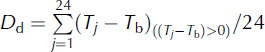. Daily degree-days, D _d, were then summed over each season. Investigating the relationship between PDDs and rift propagation events more closely, we compared our calculated PDDs with the occurrence of rift propagation events (Fig. 5). We did not observe a statistically significant correlation between the number of PDDs and timing of rift events. Days with zero propagation (and rift events that did not qualify as large) correlated with high PDD periods just as often as (if not more often than) large propagation events (Fig. 5). This suggests that large rift events are not related to rising temperatures during a season. Instead, large propagation events occurred approximately uniformly over a season, even before any positive temperatures were recorded. Using a linear regression analysis, the correlation between >0°C temperatures and the timing of rift propagation events was not calculated to be statistically significant at the 95% confidence interval.

Fig. 5.

Large propagation events vs PDDs on the Amery Ice Shelf, 2002–14. Each panel shows rift propagation rates measured between 2002 and 2014 for each rift (color-coded as Fig. 2 inset map), plotted against the number of PDDs. Yellow-circled dots signify those events that were classified as large propagation events for each rift. White squares signify those events preceded by at least 4 days of sustained high winds.

Wind speeds

We looked for a correlation between rift activity and ‘anomalous’ wind speeds, i.e. speeds two standard deviations or more above the average wind speed from 2002 to 2014. None of the large propagation events were found to coincide with anomalous winds. Using linear regression analysis, we found that that the correlation between wind speeds and rift propagation was not statistically significant, with coefficients staying close to zero (0.16 for W1, 0.11 for W2, 0.03 for T1, 0.04 for T2 and –0.5 for E3). This supports Reference Bassis, Coleman, Fricker and MinsterBassis and others (2005), who observed no instantaneous correlation between days with high winds and rift propagation in rift T2. However, Reference Bassis, Coleman, Fricker and MinsterBassis and others (2005) did observe that two out of three large ‘bursts’ in rift T2 occurred following periods of sustained strong winds. We considered sustained strong winds to be when at least four days were above average within the week prior to the rifting event. We observed that 75 of the 142 large propagation events, approximately evenly across all rifts, took place after periods of sustained strong winds, which might suggest that sustained winds may have a small influence on the timing of propagation events. However, the correlation may not be causal, in that sustained periods of high winds might also generate significant ocean swell. We consider this hypothesis next.

Sea-ice concentration

Ocean swell has been hypothesized to mechanically trigger ice-shelf rift propagation, but ocean swell can be dampened by the presence of sea ice in front of the shelf (e.g. Reference Schulz-Stellenfleth and LehnerSchulz-Stellenfleth and Lehner, 2002; Reference Bassis, Fricker, Coleman and MinsterBassis and others, 2008; Reference Bromirski, Sergienko and MacAyealBromirski and others, 2010). Both rift propagation and sea ice have strong seasonal signals. We first removed the seasonal signal from the sea-ice dataset to directly compare the variability of the sea-ice concentration and rifting rates. If sea-ice concentration controlled the propagation of rifts, we would expect that years with higher (lower) than average concentration would correlate with lower (higher) annual propagation rates in the ice shelf. While there are some years with more extreme variation (e.g. winter 2004 and summer 2002/03), for the most part sea ice oscillated from 25% to 85% concentration (Fig. 4). The correlation coefficient between the time series of rift lengths with sea-ice concentration was not statistically significant, the only exception being rift E3, which is the widest rift in our study. The satellite imagery shows that it is filled with ice melange for most of the year (Fig. 1d) and is visibly filled with sea ice for most of the year. It is possible that sea ice around or within the rift buffers the ice shelf from other influences and helps to stabilize the rift (Reference Hulbe, Ledoux and CruikshankHulbe and others, 2010). Reference Borstad, Rignot, Mouginot and SchodlokBorstad and others (2013), for example, suggested that thicker melange within a rift could be associated with less-damaged rifts. We note, however, that we have no direct observations of longer-period infra-gravity waves (e.g. Reference Bromirski and StephenBromirski and Stephen, 2012) and cannot rule out a mechanical interaction with these longer-period waves.

Arrival of tsunamis

Previously, Reference Brunt, Okal and MacAyealBrunt and others (2011) and Reference Walker, Bassis, Fricker and CzerwinskiWalker and others (2013) have documented the effect of tsunamis on front-initiated ice-shelf rifts, demonstrating that tsunami arrivals around the Antarctic continent correlated with large rift propagation events or iceberg calving events throughout the decade (2002–12). The effect appears to be most pronounced for the Amery Ice Shelf rifts. Of the 24 tsunamis that caused run-up in the Amery Ice Shelf region between 2002 and 2014 (data from the Historical Tsunami Database maintained by the US National Oceanic and Atmospheric Administration (NOAA) National Geophysical Data Center), we detected 15 instances in which one or more of the rifts propagated between documented wave arrival and the next available clear observation, limited to being within 1 month (Fig. 3). Furthermore, the abnormal winter propagation event we observed in winter 2005 is coincident with the predicted impact of two tsunamis associated with Indonesian tsunami-genic earthquakes, suggesting that these events may have been triggered by tsunami impact. Using a chi-squared test, we found that the correlation between the arrival of the tsunami and the timing of large bursts of propagation is statistically significant at the 90% confidence level.

Conclusions

We have generated time series of rift lengths for five rifts at the front of the Amery Ice Shelf using MISR and MODIS satellite imagery for the period 2002–14. While all five rifts lengthened over the observation period, the three east-propagating rifts slowed significantly after 2010, while the two west-propagating rifts continued to propagate at high rates, and have even accelerated. The average propagation rates for the period differed between rifts. Within each rift, propagation rates varied annually and exhibited a seasonal pattern, with higher rates occurring during the austral summer and almost no propagation during austral winter. We observed that nearby rifts exhibited linked behavior, with a statistically significant correlation between the timing of rift events. We also considered the occurrence of large propagation events, which dominated the seasonal averages. The number of large propagation events per rift and per season varied, and their timing was not consistent across all rifts. This observation suggests that all rifts were not responding to the same stressor; if, however, they were responding to the same stressor, the observation suggests rifts do not respond equally or synchronously to the same trigger.

We examined the possibility that propagation rates might be correlated with external environmental factors, as they clearly follow a seasonal signal. However, comparison of our rift dataset with atmospheric temperature, wind speed and sea-ice concentration does not suggest that any of these phenomena are direct triggers of rift propagation. As such, the cause of the seasonal signal remains a mystery.

The five rifts in this study are unusual in that they initiated and extend from the shelf front, rather than initiating upstream, like most other rifts observed on Antarctic ice shelves (e.g. Reference Walker, Bassis, Fricker and CzerwinskiWalker and others, 2013). The fact that structural heterogeneity, internal glaciological stress due to shelf geometry, possible sustained winds and intermittent tectonic events (by way of tsunamis) contribute to the propagation of rifts and that the rifts exhibit interactive behavior suggests that these parameters must be accounted for in modeling rift propagation in ice shelves. By continuing to observe the rifts, in the future it may be possible to connect rifting activity levels to the imminence or likelihood of large calving events.