


1. Introduction
Continental ice sheets covering Greenland and Antarctica play pivotal roles in Earth’s climate system. Deep drill cores of these ice sheets reveal they have captured and preserved their response to past climates continuously over the last one hundred thousand to one million years, providing a means to reconstruct the past to help predict future climate and project changes in ice sheet mass, geometry, and sea-level (e.g. Faria and others, Reference Faria, Weikusat and Azuma2014; Lauritzen and others, Reference Lauritzen2025). Reconstructions of climate records and ice dynamics use the same archive of ice core layers and are interdependent in many ways. That is, when these layers formed through the burial and compaction of recurrent snowfalls, they trapped ancient atmospheres in the form of air bubbles, airborne particles, and elemental and isotopic abundances, but interpreting their stratigraphic chronology relies on our understanding of ice grain mechanics and interactions with these climate proxies (e.g. Faria and others, Reference Faria, Freitag and Kipfstuhl2010, Reference Faria, Weikusat and Azuma2014; NEEM community members, 2013; Stoll and others, Reference Stoll, Eichler, Hörhold, Erhardt, Jensen and Weikusat2021; Westhoff and others, Reference Westhoff2021). More specifically, how microstructural mechanisms facilitate the creeping flow of ice sheets at the crystal-scale not only informs the origin and integrity of ice core stratigraphy but also allows large-scale ice sheet evolution and its climatic effects to be modeled (Fan and Prior, Reference Fan and Prior2023; Gerber and others, Reference Gerber2023; Zhang and others, Reference Zhang2024). Our ability to interpret such information, however, fundamentally relies on our approach to textural analysis (grain and bubble morphologies, sizes, orientations) and how we access ice layers to begin with.
Since polar ice core drilling began in the 1950s, scientists have accessed thousands of meters of ice sheet stratigraphy by developing what are now standard core-processing techniques. These include an assembly line of instruments and saws to measure along-core properties and to send samples to various labs for gas, chemistry, and isotope analysis. Although traditional sample preparations and analytical techniques involve dissection of the ice cores and can remove important three-dimensional (3D) context (Westhoff and others, Reference Westhoff2021; Disbrow-Monz and others, Reference Disbrow-Monz, Hudleston and Prior2024), one-dimensional (1D) and two-dimensional (2D) analyses have led to detailed climate-record reconstructions and form the basis of most textural studies carried out to date (e.g. Gow and Williamson, Reference Gow and Williamson1976; Lipenkov and others, Reference Lipenkov, Barkov, Duval and Pimienta1989; Thorsteinsson and others, Reference Thorsteinsson, Kipfstuhl and Miller1997; Svensson and others, Reference Svensson, Baadsager, Persson, Hvidberg and Siggaard-Andersen2003a; Durand and others, Reference Durand, Gagliardini, Thorsteinsson, Svensson, Kipfstuhl and Dahl-Jensen2006; Binder and others, Reference Binder, Garbe, Wagenbach, Freitag and Kipfstuhl2013; Montagnat and others, Reference Montagnat2014a; Fan and others, Reference Fan2021; Stoll and others, Reference Stoll2025). A question remains, however, as to what scientists can learn if they initially and routinely have access to ice core textures in 3D.
Progress towards 3D characterizations of snow and ice textures have been made over the last two decades using X-ray microtomography. Air bubbles in deep ice cores are often relatively easy to wholly visualize by X-ray attenuation given their small scale and low density compared to ice grains, making it possible to measure porosity and contextualize trapped greenhouse gases (Burr and others, Reference Burr, Ballot, Lhuissier, Martinerie, Martin and Philip2018; Baker, Reference Baker2019). However, in both synchrotron- and lab-based X-ray systems, challenges surrounding the necessary cold analytical environments and sample size limitations mean that sufficient grain numbers with crystal orientation measurements have not been achieved (e.g. Flin and others, Reference Flin, Brzoska, Lesaffre, Coléou and Pieritz2004; Schneebeli and Sokratov, Reference Schneebeli and Sokratov2004; Kaempfer and Schneebeli, Reference Kaempfer and Schneebeli2007; Heggli and others, Reference Heggli2011; Rolland du Roscoat and others, Reference Rolland du Roscoat2011; Riche and others, Reference Riche, Montagnat and Schneebeli2013; Granger and others, Reference Granger, Flin, Ludwig, Hammad and Geindreau2021).
However, crystal orientations are thought to play a critical role in ice sheet evolution, which begins with the intrinsic visco-plastic anisotropy of each ice crystal’s hexagonal structure (Duval and others, Reference Duval, Ashby and Anderman1983; Fan and others, Reference Fan2021; Fan and Prior, Reference Fan and Prior2023). The basal plane in ice has a relatively low resistance to shear, thus the gravity-driven flow occurring in ice sheets causes dislocation slip mainly along the basal plane, while the crystal c-axis tends toward the compressive-stress direction (Gow and Williamson, Reference Gow and Williamson1976; Alley, Reference Alley1992). This leads to a bulk anisotropy manifesting in crystallographic fabrics that develop under continued snow deposition, burial, and ice deformation (Gow and Williamson, Reference Gow and Williamson1976). In effect, feedback occurs between fabrics and flow, such that crystal orientations control the bulk mechanical behavior of the polycrystalline ice, but the fabrics also evolve as a function of the ice’s thermomechanical history. Therefore, crystal orientations exert an important rheological control on the large-scale flow of ice sheets (Duval and others, Reference Duval, Ashby and Anderman1983; Shoji and Langway, Reference Shoji and Langway1985; Castelnau and others, Reference Castelnau1998; Gerber and others, Reference Gerber2023; Rathmann and others, Reference Rathmann, Lilien, Richards, McCormack and Montagnat2025).
Depending on the extent and mechanisms of ice deformation, the fabric-induced mechanical anisotropy of the ice layers can vary considerably over the depth of the ice column (Thorsteinsson and others, Reference Thorsteinsson, Kipfstuhl and Miller1997; Montagnat and others, Reference Montagnat2014a; Montagnat and others, Reference Montagnat, Löwe, Calonne, Schneebeli, Matzl and Jaggi2020; Stoll and others, Reference Stoll2025). For this reason, crystal orientation measurements are routinely performed with automatic fabric analyzers (AFAs) or other mapping methods that rely on optical microscopy and cm-scale, 2D thin sections of ice cores (Wilson and others, Reference Wilson, Russell-Head and Sim2003; Kipfstuhl and others, Reference Kipfstuhl2006). Although these are high-resolution methods and can rapidly measure c-axis directions for hundreds of grains, they cannot determine directions of the three a-axes for each grain (Wilen and others, Reference Wilen, Diprinzio, Alley and Azuma2003; Wilson and others, Reference Wilson, Peternell, Piazolo and Luzin2014). This leaves consequential gaps in textural data, such as whether grains are truly distinct from one another outside the section plane (Disbrow-Monz and others, Reference Disbrow-Monz, Hudleston and Prior2024), or whether a-axis directions can or should be used as strain markers to understand ice flow (Qi and others, Reference Qi2019; Hunter and others, Reference Hunter, Wilson and Luzin2023; Lilien and others, Reference Lilien2023). Furthermore, an incomplete understanding of how to efficiently parameterize the elastic and visco-plastic anisotropies of individual grains partly prevents ice-flow models from accounting for their effects, at least to the desired accuracy (Ranganathan and others, Reference Ranganathan, Minchew, Meyer and Peč2021; Richards and others, Reference Richards, Pegler, Piazolo and Harlen2021; Lilien and others, Reference Lilien2023; Ranganathan and Minchew, Reference Ranganathan and Minchew2024). At present, coupling small-scale micromechanical models with large-scale ice-flow models is rarely considered for two main reasons. First, it has proven challenging to incorporate realistic, yet efficient, representations of crystal fabrics into large-scale models (e.g. Montagnat and others, Reference Montagnat2014b; Lilien and others, Reference Lilien2023). Second, only a few ways have been proposed to parameterize the predictions made by micromechanical models, each with their own caveats and limitations (Gillet-Chaulet and others, Reference Gillet-Chaulet, Gagliardini, Meyssonnier, Montagnat and Castelnau2005; Placidi and others, Reference Placidi, Greve, Seddik and Faria2010).
In addition to crystal-orientation fabrics, more work is needed to understand the influence of grain sizes, shapes, boundaries, and even bubbles on ice metamorphosis and how they should also be parameterized in models (Kuiper and others, Reference Kuiper, Weikusat, De Bresser, Jansen, Pennock and Drury2020). However, collecting this microstructural information has proven challenging for polycrystalline ice. Optical and cryo-electron backscatter diffraction (EBSD) techniques provide visibility of ice grain boundaries, but only in 2D (e.g. Iliescu and others, Reference Iliescu, Baker and Chang2004; Piazolo and others, Reference Piazolo, Montagnat and Blackford2008; Prior and others, Reference Prior2015). Whereas, X-ray tomography provides 3D context but traditionally necessitates X-ray diffraction from mm-scale samples to distinguish individual grains (Baker, Reference Baker2019). Ultimately, gaining the ability to correlate 3D behaviors of microstructures and bubbles in ice cores over large sample volumes could improve both paleoclimate reconstructions and the physical realism of large-scale ice-flow models.
Here we present a new non-destructive 3D method for the textural analysis of ice cores that complements standard methods used in ice core studies. By implementing well-established grain-mapping techniques that have been transferred from the synchrotron to the lab (e.g. Juul Jensen and others, Reference Juul Jensen2006; Ludwig and others, Reference Ludwig, Schmidt, Lauridsen and Poulsen2008; King and others, Reference King, Reischig, Adrien, Peetermans and Ludwig2014; McDonald and others, Reference McDonald2015), our method makes it possible to simultaneously map ice grains and pore spaces in 3D while measuring their volumes and shapes with respect to complete crystallographic orientations of the grains. Our method combines two lab-based X-ray modalities—absorption contrast tomography (ACT) and diffraction contrast tomography (DCT)—which enable the visualization, measurement, and spatial correlation of ice grain and air bubble textures, adding new perspectives on ice core stratigraphy and new ways to access modeling parameters. We achieve this by pushing the spatial resolution and sample volume limits of DCT in the lab and by mitigating challenges in X-ray diffraction posed by crystal deformation. Our measurement approach is based upon a specially designed cooling device that accommodates ∼3 × 3 × 3 cm3 samples containing hundreds to thousands of grains, extending observational volumes of ice by one to four orders of magnitude over those quoted 5–30 years ago (e.g. Liu and others, Reference Liu, Baker, Yao and Dudley1992, Reference Liu, Baker and Dudley1995; Rolland du Roscoat and others, Reference Rolland du Roscoat2011; Baker, Reference Baker2019). To demonstrate the power of greater spatial and statistical information, we evaluate the representation of grain size distributions and orientations in 3D versus 2D, investigate grain and bubble relationships in 3D, and discuss the relevance of complete 3D crystallographic information in constraining micromechanical models that underpin current large-scale ice-flow models.
2. Methods
2.1. Building a freezer inside the laboratory X-ray microscope
A cooling device was designed at Lund University under the requirement that it (1) keeps ice at a temperature well below −10°C and (2) maximizes sample size while minimizing grain diffraction overlap, which we simulated beforehand. A sketch of the experimental set-up is shown in Fig. 1. Each sample sat directly on a 34 mm-diameter aluminum plate that was cooled by a Peltier element. The hot bottom-side of the Peltier was kept cold using an external chiller, attached to the device through an integrated slip ring system that held fluid hoses stationary during sample rotation. Sample housing above the plate included a 27 mm-tall polymer (PMMA) tube with 3 mm-thick walls, as well as surrounding polyethylene foam with 13 mm-thick walls, bringing the total housing diameter to 66 mm. For 30 min, chiller fluid cooling to 5°C was circulated through the device before powering the Peltier and setting it to −35°C, an unobtainable target that prevented temperature regulation. Plate sensor readings reached −29°C in 10 min and remained stable below each sample during data acquisition (up to 24 h). A sensor embedded 3 mm beneath the upper sample surface also read stable at −21°C during a test. While not ideal, thermal gradients of ∼0.3°C mm−1 along the ∼3 cm sample height had negligible effects on ice microstructures at these temperatures and on our analytical timescales. Air temperatures between the upper sample surface and insulating foam reached −14°C in 5–7 min and typically continued to decrease by a few degrees.
The cooling device, sample and beam geometries used for lab-based multimodal X-ray imaging. Examples of absorption and diffraction contrast projection data shown here correspond to a subvolume of a firn sample described in Section 2.2. Source-to-sample and sample-to-detector distances are referred to as DS-S and DS-D, respectively, and are provided in Section 2.3.

2.2. Selecting and working with ice core samples
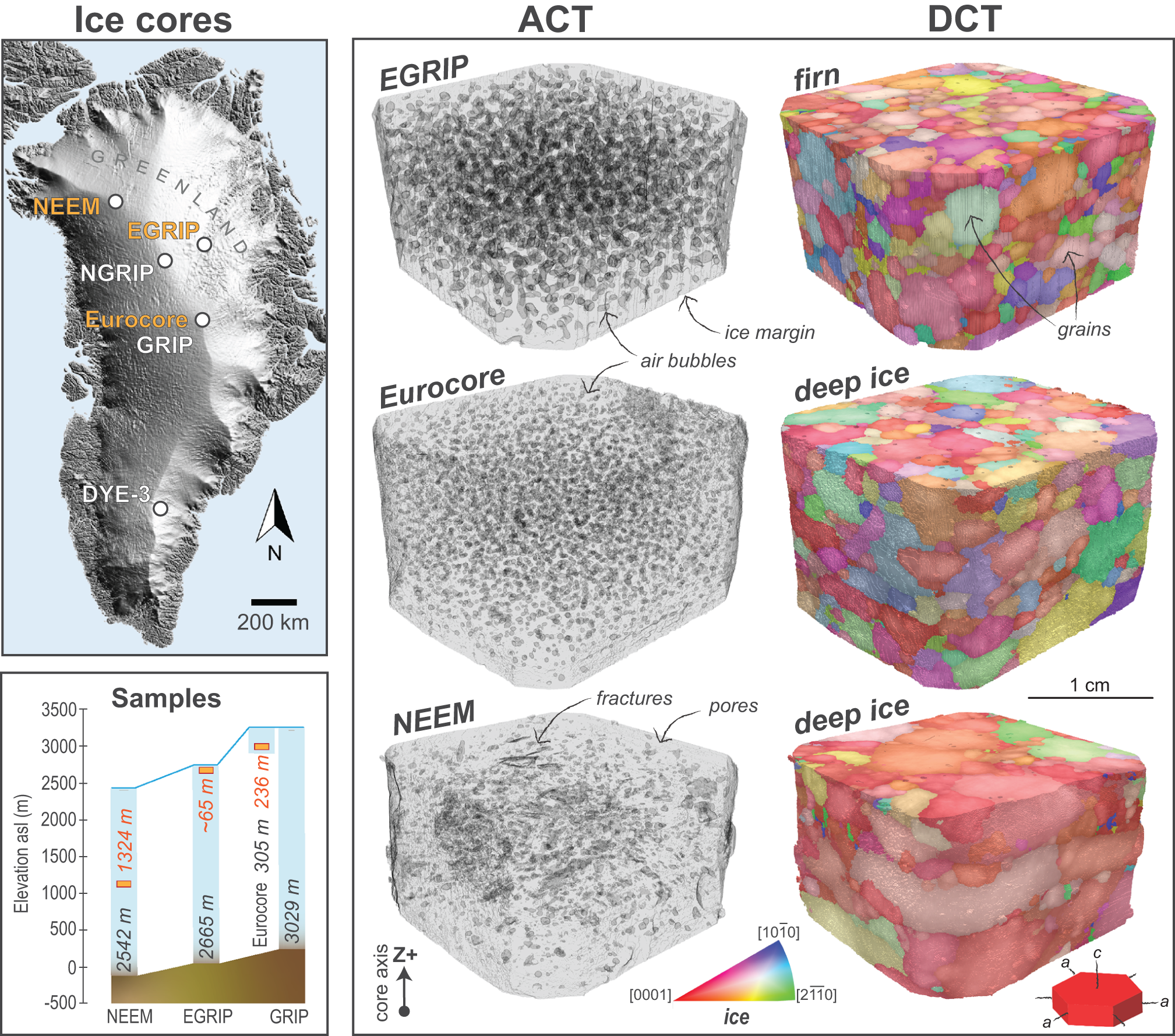
We selected 10 samples from the Niels Bohr Institute’s ice core archive at the University of Copenhagen. Samples include firn and Holocene-age deep ice from central, northwestern, and southern drilling sites on Greenland (i.e. EGRIP, Eurocore, NEEM, and Dye-3; Fig. 2). For experimental purposes, we targeted non-precious cores that had suffered drilling and recovery complications in the field. Of the samples, we focused on three that cover a range in depth and enabled us to develop methods and establish proof of concept (Fig. 2; Table 1). Each sample captures less than 1 year, and in some cases less than one winter or summer season, based on its thickness (0.03 m) and the annual ice-layer thickness at the depth it was extracted from. The original cores have been stored at −30°C for durations that can be deduced from their drilling dates in Table 1.
Overview of the three ice-core sample datasets used for method development. We screened samples from five ice-core drilling sites shown on the DEM of Greenland. In this paper, we present sample data from the sites labeled in orange (also see Table 1). Sample depths are provided with elevations and the final core depths at those drilling sites. EastGRIP was drilled between 2016 and 2023 within the active Northeast Greenland Ice Stream (NEGIS). The depth of the EGRIP firn sample is estimated based on sample porosity and firn density profiles of NEGIS (Vallelonga and others, Reference Vallelonga2014). Eurocore was drilled in 1989, just 30 m away from the GRIP site (GReenland Ice core Project, drilled 1990–1992). Our deepest sample is from the NEEM core (North Greenland Eemian ice drilling project), drilled between 2009 and 2012. The observed differences in porosity and grain sizes between the three samples generally reflect their different depths within the ice sheet.

Details of Holocene samples from Greenland ice cores.

a Mojtabavi and others (Reference Mojtabavi2020).
b Seierstad and others (Reference Seierstad2014).
c Rasmussen and others (Reference Rasmussen2013).
Sections of the 10 cm-diameter cores were sawn inside a walk-in freezer at the University of Copenhagen and cut into smaller, ∼3 × 3 × 3 cm3 samples (Fig. 1). The samples were then sealed in plastic bags and transported for 1 h by cooler box to Xnovo Technology in Køge, Denmark for X-ray imaging. The cooler box and its contents were stored for a few days to months between −20°C and −25°C inside a small, temperature-monitored freezer next to the X-ray microscope. Ice exposure to room temperature lasted 2–4 s when samples were transported by cold steel tweezers into the X-ray microscope cabinet. Mounted samples were frozen to the aluminum plate using one drop of water, which temporarily increased the plate temperature by 1°C. No ice metamorphosis occurred before or during data acquisition, although an inconsequential <2 mm layer of frost commonly accumulated on sample surfaces while inside the cooling device.
2.3. Absorption and diffraction contrast tomography
Ice textures were characterized through correlative, multimodal X-ray imaging using a Zeiss Xradia 520 Versa X-ray microscope equipped with a LabDCT Pro module. ACT was used to visualize sample morphology and determine the shapes of pore spaces, including trapped (primary) air bubbles and secondary pores and fractures. Whereas, DCT was used to measure and map 3D crystallographic orientations and shapes of grains. Grains can only be defined by DCT, because they lack contrast in ACT due to their same composition and density. The crystal lattice distortion inherent to glacial processes prompted us to explore different X-ray scanning conditions to optimize data collection from grains that are plastically deformed, a general challenge in X-ray diffraction methods (Fig. S1).
To optimize absorption contrast between ice and pore spaces, ACT scans were performed at 80 kV and 7 W. We placed the X-ray source at 61 mm and detector at 245 mm away from the sample to maximize spatial resolution while avoiding hardware collision with the cooling device (Fig. 1). These distances created a geometrical magnification of 5x that corresponded to a large, roughly 46 × 29 mm2 field of view on the flat panel detector, which, as a result, produced a tomography image containing 3064 × 1936 pixels at a nominal size of 75 µm and effective size of 14.95 µm. We collected 3201 projections (images), each with 0.5 s of exposure, as the sample completed a 360° rotation. This ACT acquisition step took less than 2 h.
Directly after the ACT scan, we performed the correlative DCT scan. Given that many grains lie in the X-ray beam’s path, we optimized diffraction patterns for crystallographic reconstruction by performing DCT scans (110 kV, 10 W) with the flat panel detector in a projection geometry close to Laue focusing (Bachmann and others, Reference Bachmann, Bale, Gueninchault, Holzner and Lauridsen2019), such that source-to-sample (200 mm) and sample-to-detector (245 mm) distances were similar enough to produce radially focused, linear diffraction spots that reduced spot overlap (Fig. 1). Two different source-beam apertures were used depending on the extent of grain deformation, which causes a radial spread of cloudy and elongated diffraction spots, known as asterism (Fig. S1). A 375 × 375 µm2 square aperture was used for firn and deep ice from <300 m depths. Whereas, a 200 µm circular pinhole aperture improved results for much deeper (1000s of meters) and more deformed ice by (1) illuminating less sample volume per projection and (2) improving diffraction spot definition by constraining spots to the aperture’s pinhole shape. Depending on the aperture used, our source distance gave roughly a 9 × 9 mm2 to 5 × 5 mm2 field of view. To keep experiment times to a day, partial sample volumes of approximately 3 × 3 × 1.7 cm3 were covered in one advanced helical phyllotaxis raster scan (Oddershede and others, Reference Oddershede, Bachmann, Sun and Lauridsen2022) consisting of 1119 to 5061 projections, each with an exposure time of either 5 or 10 s for the larger aperture and 10 s for the pinhole. The DCT acquisition step took approximately 5–6 h when using the larger aperture and 20 h using the pinhole. From start to finish, each multimodal imaging measurement was completed in ∼8–24 h.
2.4. Data reconstruction and processing
2.4.1. Ice and pore volumes
We reconstructed sample volumes from the ACT data using cubic voxels with side-lengths of 14.95 µm. This was performed using a filtered back projection routine and the reconstructor tool in ZEISS Scout-and-Scan software. Because individual ice grains have the same density, they cannot be distinguished by way of X-ray attenuation and thus form one continuous volume with homogeneous grayscale intensity. Much lower density air bubbles >40 µm in diameter and apparent microfractures were detectable at the reconstructed voxel size, while dust impurities, which are typically on the order of a few micrometers, fell below the detection limit.
2.4.2. Ice grain crystallographic orientations and morphologies
Using Xnovo Technology’s GrainMapper3D software, crystallographic maps were reconstructed from the DCT data with 60 µm-wide cubic voxels inside the volume mask obtained from the ACT data (Bachmann and others, Reference Bachmann, Bale, Gueninchault, Holzner and Lauridsen2019; Fig. 2). Natural ice on Earth occurs as ice Ih (ice one hexagonal), which belongs to the hexagonal crystal system and dihexagonal dipyramidal 6/mmm Laue class (and point group). Lattice parameters for space group P63/mmc of a = 4.489 Å, c = 7.327 Å and the four {hkil} families { $2\overline {11} 0$}, { $10\bar 10$}, { $10\bar 13$}, and { $2\overline {11} 2$} were used to reconstruct ice grains from diffraction patterns. We use Fig. 3 to show how we define grains and subgrains in our data. Adjacent regions in 3D space were assigned to the same ‘grain’ if the voxel-to-voxel, crystallographic angular misorientation was <2° (EGRIP firn, Eurocore deep ice) or <3° (NEEM deep ice). The reason for using different thresholds for different samples relates to their amount of deformation, its impact on diffraction pattern quality, and therefore the confidence in grain detection and reconstruction. Lower misorientation thresholds yielded large numbers of low confidence grains a few hundred microns in size, which were interpreted to be unphysical. Therefore, grain maps were cleaned by replacing any grain with a neighboring grain that it shared the largest boundary area with, based on fulfillment of at least two of the following three criteria indicative of poor reconstruction: (1) a mean completeness of <60% across the grain (completeness is defined as the ratio between the number of observed and expected diffraction spots for a given orientation); (2) a grain volume less than 83 = 512 voxels (equivalent sphere diameter < 600 µm); (3) a misorientation to a neighbor-of-a-neighbor grain of < 2° (EGRIP firn, Eurocore deep ice) or < 4° (NEEM deep ice). These limits ensured the merging of high confidence grains with low confidence grains located at their boundaries and with misorientations close to the set threshold.
Grain and subgrain definition in this study. Grains were reconstructed based on our chosen scanning conditions and crystallographic misorientation thresholds described in the Methods. Virtual slices of 3D grain maps of the EGRIP firn sample are used here for demonstrative purposes, wherein we defined grains based on a 2° misorientation threshold. Grain completeness typically drops both at grain and subgrain boundaries, enabling their visualization. This is because of the 1:1 relationship between the shapes of diffraction spots on the detector and the shapes of the diffracting volumes (i.e. grains or subgrains), with the spot edges corresponding to grain and subgrain boundaries. As a note, the completeness map underlies all other maps shown in the top row. The grain definition map reflects our chosen misorientation threshold to define grains, resulting in groupings of adjacent regions defined by completeness drop-off and circled in black. When looking at IPF maps for XYZ directions, regions defined as one grain appear with the same IPF color, consistent with the grain definition map. IPF coloring may be similar for neighboring grains above the chosen misorientation threshold, such as those circled by red-dashed lines. The grain reference orientation deviation (GROD) and grain orientation spread (GOS, or average GROD) maps verify that apparent subgrains identified in previous maps can be interpreted as such, given that the locations of completeness drop-off correspond to low-angle misorientation boundaries.

Using GrainMapper3D, we validate the reconstruction of both non-deformed and deformed grains by inspecting forward projections of the {hkil} families listed above (see Bachmann and others, Reference Bachmann, Bale, Gueninchault, Holzner and Lauridsen2019 for details). As seen in Fig. S1, forward projection outlines cover the spread in orientation represented by elongated diffraction spots that originate from deformed grains. When we define a deformed grain (i.e. consider the deformed grain to be one grain with one orientation), it becomes the average orientation (or the average forward projection), which can also be seen in Fig. S1. Although the current reconstruction model does not account for lattice deformation, it can be tolerated so long as diffraction spots can be clearly extracted and separated (Bachmann and others, Reference Bachmann, Bale, Gueninchault, Holzner and Lauridsen2019). Resolving subdomains or subgrain boundaries is dependent on use of the Laue-focusing geometry (increases angular sensitivity), working distances, and grain and sample sizes (Bachmann and others, Reference Bachmann, Bale, Gueninchault, Holzner and Lauridsen2019). We calculated crystallographic misorientations using the difference between a reconstructed grain’s average orientation and the orientations of individual voxels composing that grain (i.e. the grain reference orientation deviation, or GROD). Because we considered adjacent voxels with <2–3° misorientations to be the same ‘grain’, the maximum misorientations of subgrains with low-angle grain boundaries were defined to be <2° or <3°, depending on the specific sample. We show in Fig. 3 that combined maps of completeness, inverse pole figures (IPFs), and grain reference orientation deviations (GRODs) can be used to characterize subgrains. The uncertainty in grain boundary position is approximately 5–10% of the grain size and is related to the diffraction spot size and their binarization in our data (cf. Bachmann and others, Reference Bachmann, Bale, Gueninchault, Holzner and Lauridsen2019). For spots originating from deformed grains, this uncertainty can be greater and needs to be quantified and statistically assessed in the future.
2.5. Data analysis and visualization
Our analysis was focused on demonstrating the complementarity of 3D and 2D data, as well as the new possibilities offered by 3D data available through our method. Therefore, the analysis is limited in scope regarding ice mechanics and climate records. We instead focus on comparing traditional and new perspectives using a few of the most common types of texture analyses performed on ice cores. All analyses and 3D visualizations were generated using in-house code at Xnovo Technology, GrainMapper3D (Bachmann and others, Reference Bachmann, Bale, Gueninchault, Holzner and Lauridsen2019), Paraview (Ayachit, Reference Ayachit2015), or the Python package Vedo (Musy and others, Reference Musy2025).
2.5.1. Grain sizes
Grain size statistics were derived from both 3D reconstructed volumes and 2D cross-sectional slices for comparison. Two grain metrics, the equivalent grain diameter and major-axis length, were chosen to demonstrate the comparisons in Figs. 4 and 5 (also see Fig. S2). For each grain and each slicing axis (X, Y, Z), the mean, minimum, and maximum values of the chosen 2D metric across all slices intersecting that grain were calculated. In the generated scatter plots, each point represents a single grain, with the 3D metric value compared to the mean 2D metric value calculated from all slices intersecting the grain, either along a specified slicing axis or XYZ axes combined. Vertical bars were added to each point (grain) to indicate the minimum and maximum 2D metric value observed when slicing along a specified axis. Additionally, grain size distributions based on the equivalent diameter were visualized through histograms that emphasize the contribution of different sizes to the total volume (for 3D) or total area (for 2D slices). For demonstrative purposes, grain-related analyses include grains that intersect the sample margins due the presence of larger grain sizes (cf. Svensson and others, Reference Svensson, Baadsager, Persson, Hvidberg and Siggaard-Andersen2003a).
Comparing grain size information between 3D grain maps and virtual 2D slices of the EGRIP firn sample. (a) The 3D grain map, colored by grain diameter, was sliced orthogonally. (b) Grain size distributions based on 3D data are compared to those calculated in single, orthogonal X and Z section planes through the sample, which simulate vertical (X) and horizontal (Z) cuts typically made of ice cores. (c) Multiple XYZ slices in these plots represent 60 µm intervals (i.e. the reconstructed voxel size of DCT data). Grain sizes calculated from 3D volumetric data are plotted against grain sizes calculated from combined XYZ orthogonal slices, hence the 1:1 line, as well as the average 2D size of each grain found across XYZ slices combined. Each grain’s average size based on either all X-slices or all Z-slices is also compared to its volume-calculated size, with the full 2D size range for each grain plotted as vertical bars. Note that all plot diameters represent equivalent sphere (3D) or circle (2D) diameters.

Comparing grain size information between 3D grain maps and virtual 2D slices of the NEEM deep ice sample. (a) The 3D grain map, colored by grain diameter, was sliced orthogonally. X and Z slices simulate the typical vertical (X) and horizontal (Z) cuts made of ice cores. (b–c) Multiple XYZ slices in these plots represent 60 µm intervals (i.e. the reconstructed voxel size of DCT data). Grain sizes calculated from 3D volumetric data are plotted against grain sizes calculated from combined XYZ orthogonal slices, hence the 1:1 line, as well as the average 2D size of each grain found across XYZ slices combined. Each grain’s average size based on either all X-slices or all Z-slices is also compared to its volume-calculated size, with the full 2D size range for each grain plotted as vertical bars. Note that (b) plots diameters as equivalent sphere (3D) or circle (2D) diameters, whereas (c) plots the major-axis lengths of grains based on ellipsoid (3D) and ellipse (2D) fitting.

2.5.2. Grain orientations
Pole figure analysis involved plotting separately: (1) the number-weighted grain orientations; (2) the volume-weighted grain orientations; and (3) all grains compared to those of separate grain size fractions for (1) and (2) (Figs. 6 and 7). To do this, we plotted and symmetrized discrete c-axis and a-axes directions for each grain within the sample reference frame (XYZ). The kernel density of the distribution of crystal axis directions was estimated using a de La Vallee Poussin kernel with a halfwidth (kappa, K) of 10° and weighting them by number or volume. A unit sphere grid with density weights was plotted in a filled tri-contour plot in an equal-angle, lower-hemisphere stereographic projection.
Comparing pole figure analyses for the Eurocore sample’s grain orientations based upon count, volume, and grain size fraction. Pole figures provide views down the sample Z-axis, parallel to the ice core axis. Analytical details are provided in the Methods. Note that glaciological studies employing EBSD of ice may instead represent the a-axes as [ $11\bar 20$] (−a 3), which is symmetrically equivalent to [ $2\overline {11} 0$] (+a 1) (e.g. see Qi and others, Reference Qi2019).

Comparing pole figure analyses for the NEEM sample’s grain orientations based upon count, volume, and grain size fraction. Pole figures provide views down the sample Z-axis, parallel to the ice core axis.

2.5.3. Pore positions and shapes
Pore analysis in 3D leveraged complementary information from ACT and DCT datasets. To gain insight into spatial relationships between pores and grains, we correlated ACT segmentation and DCT grain labels. After segmenting pores from the ACT volume, a connected components analysis (26-connectivity) and 5-voxel minimum was used to identify individual pores and calculate their voxel count, volume, equivalent sphere diameter, and centroid. Pore-grain adjacency was then determined relative to the DCT grain map, such that the neighborhood of each identified ACT pore was examined within the corresponding region of the DCT volume. The pore–grain adjacency was visualized by generating a surface mesh of grains in the DCT volume (colored by IPF crystallographic orientations) and overlaying it with the ACT-derived pore mesh (one color, gray), which made pore and grain boundary surfaces visible. These surfaces provided a visualization of ACT pores colored by the IPF orientation of their host grain(s). We then characterized pores based on their position and size with respect to grain boundaries, classifying them as ‘intragranular’ or ‘intergranular’ based on the number of unique adjacent DCT grain labels detected in a 3 × 3 × 3 (ACT) voxel-dilated boundary around each pore. In the EGRIP firn sample, where the average pore size is 1 mm and most grains are smaller than 10 mm, the pore classification is highly accurate considering the estimated uncertainty on grain boundary position is 5–10% of the grain size. The pore classification is considered less accurate in our Eurocore and NEEM data due to a combination of smaller pores and larger, more deformed grains. Counts and sizes of total, intragranular, and intergranular pores were analyzed statistically. Pores that intersect sample margins had a negligible effect on the analytical results.
To characterize each pore based on its shape and size, we made principal measurements using ACT data and performed a convex hull fitting with a ‘minimum volume enclosing ellipsoid’ containing a set of points. Fitted axis measurements were made for ellipsoids following the axis convention a ≥ b ≥ c [where ellipsoid factor, EF = c/b − b/a, and the aspect ratio is a/c]. These measurements include axis length (L) and corresponding azimuth (φ) and elevation (θ) after rotation. Analyses focused on measuring the extent and direction of pore flattening or elongation with respect to the host grain’s c-axis direction, as well as the sample compression axis (Z), which is parallel to the ice core axis. Only intragranular pores were considered for the purpose of comparing results to those of Fegyveresi and others (Reference Fegyveresi, Alley, Voigt, Fitzpatrick and Wilen2019), who focused on intragrain deformation. Therefore, the intergranular pores touching grain boundaries were excluded entirely from our shape-related analyses, while the intragranular pores were also filtered to exclude those intersected by sample margins.
3. Results and discussion
3.1. Visualizing ice grains and pores through correlative 3D images
Herein we demonstrate some of the utility of lab-based, multimodal (ACT + DCT) X-ray tomography for the 3D analysis of ice cores. For brevity, we focus on one firn sample and two deep ice samples that cover a range in depth and metamorphosis, as exemplified by differences in their porosities, grain sizes, shapes, and crystallographic orientations visible in Fig. 2. Again, reconstructing and correlating images of these parameters required the consecutive collection of X-ray absorption and diffraction image data. When correlating the two image types, pores and ice grains are numerable and their spatial characteristics and relationships measurable in 3D. Notably, the correlated images enable fast qualitative assessments of ice core textures that can guide and contextualize measurements.
Prior to any quantitative analysis, there is visible evidence of crystallographic preferred orientations (CPOs) in the IPF maps in Fig. 2. These maps are colored with respect to the ‘up’ or vertical (Z+) direction of ice cores, perpendicular to the glacier surface. The dominance of red indicates a c-axis preferred orientation, such that many grains are oriented with the axis near-vertical. These observations match those commonly made from AFA images of thin sections (e.g. Faria and others, Reference Faria, Weikusat and Azuma2014). The correlative maps also allow qualitative observations of a-axis CPOs, as well as volumetric differences in porosity and grain sizes between different samples.
For the samples we considered and the ∼12–15 cm3 volumes we correlated, we observed representative air bubble sizes, shapes, and distributions, but capturing representative grain sizes was challenging, as large grains can intersect sample margins or extend beyond imaged volumes. Our observations are corroborated by previous documentations of bubbles, which reach just tens of micrometers to millimeters in size beneath the lower part of the firn-column, where bubbles become closed-off (e.g. Bendel and others, Reference Bendel2013; Westhoff and others, Reference Westhoff2024). In contrast, ice grains can reach centimeters at depth and even meters near warm bedrock (Baker, Reference Baker2019). While we achieve a total sample size of ∼3 cm tall × ∼3 cm diameter, which is much greater than sizes attempted previously in synchrotron- and lab-based multimodal experiments (e.g. 2 mm thick up to 1 × 1 cm; Liu and others, Reference Liu, Baker, Yao and Dudley1992, Reference Liu, Baker and Dudley1995; Jia and others, Reference Jia, Baker, Liu and Dudley1996; Rolland du Roscoat and others, Reference Rolland du Roscoat2011), we acknowledge that even larger samples would be ideal for accurate characterizations of coarse-grained ice. However, larger samples equate to measurement limitations, ranging from too many diffracting grains crowding the X-ray detector, to resolution limits and long acquisition times.
Analyzing ice cores with grain sizes too large to capture whole is a problem for all existing methods. When using optical microscopy and thin sections, the problem may be compounded by irregular grain shapes, such that duplicated measurements of grains appearing more than once in the section will influence CPO analysis (Svensson and others, Reference Svensson2003b; Monz and others, Reference Monz2021). Furthermore, although cryo-EBSD has been applied to serial sections of coarse-grained ice to identify representative volumes, shapes, and sufficient grain numbers needed for accurate CPO characterizations, this is labor-intensive and can create positional and angular uncertainties when recombining sections and stitching data together (Monz and others, Reference Monz2021). We note that a stitching approach can also be taken with our X-ray method using serially cut ice blocks, which, when combined with recent advancements in 3D image correlation, could eliminate many uncertainties and address large grain sizes. Effectively, the sample volumes we imaged here balance the pros and cons of relatively large samples for lab-based DCT and provide the option to collect lower- versus higher-resolution data to fit scientific questions.
3.2. Contrasts between 3D and 2D grain size distributions
Ice rheology has both crystal orientation and grain size dependencies (Cuffey and others, Reference Cuffey, Thorsteinsson and Waddington2000; Durand and others, Reference Durand, Gagliardini, Thorsteinsson, Svensson, Kipfstuhl and Dahl-Jensen2006). How these characteristics vary across ice layers largely reflects the deformation mechanisms driving the viscous flow of ice sheets under their own weight (Thorsteinsson and others, Reference Thorsteinsson, Kipfstuhl and Miller1997; De La Chapelle and others, Reference De La Chapelle, Castelnau, Lipenkov and Duval1998; Ranganathan and others, Reference Ranganathan, Minchew, Meyer and Peč2021). Crystal orientation fabrics and grain sizes, however, are commonly decoupled (Svensson and others, Reference Svensson, Baadsager, Persson, Hvidberg and Siggaard-Andersen2003a; Wang and others, Reference Wang, Kipfstuhl, Azuma, Thorsteinsson and Miller2003; Stoll and others, Reference Stoll2025). In thin sections, the cross-sectional areas and shapes of grains change depending on burial depth, temperature, amount of shear, or impurity concentrations. Observed trends between grain area (2D) distributions and depth have led to informative grain growth models, although it has been acknowledged that grain volume (3D) data would better suit these models (Svensson and others, Reference Svensson2003b).
Figures 4 and 5 demonstrate how volumetric data from 3D grain maps can be used to assess the representativeness of 2D grain size distributions, which are the standard calculations typically made using vertically, and sometimes horizontally, cut surfaces of ice cores (Faria and others, Reference Faria, Weikusat and Azuma2014). While there are many ways glaciologists go about these calculations, we chose to compare 3D and 2D grain size distributions by calculating equivalent sphere and circle diameters of grains from their volumes and cross-sectional areas, respectively. We also extract the major- and minor-axis lengths of grains based on ellipsoid (3D) and ellipse (2D) fitting. We show in Figs. 4 and 5 how vertical and horizontal cuts can impose bias on grain size measurements and related calculations (also see Figs. S2 and S3). This is a well-known problem that continues to motivate refinement of statistical correction methods, as a single 2D measurement cannot capture the full grain shape and must be based on additional assumptions (e.g. Morgan and Jerram, Reference Morgan and Jerram2006; Mangler and others, Reference Mangler, Humphreys, Wadsworth, Iveson and Higgins2022; Bretagne and others, Reference Bretagne, Wadsworth, Vasseur and Dobson2023). To demonstrate this dimensional bias statistically, we digitally cut the sample volume into vertical and horizontal serial sections at intervals equal to the 60 µm voxel size of the DCT grain map. This enabled us to measure the mean circle (2D) diameter of each grain against its spherical (3D) diameter, while noting the full range of circle diameters encountered (Figs. 4 and 5). We find that, on average, grain sizes would be severely underestimated in vertical cuts of our samples, whereas grain sizes in horizontal cuts would be comparatively more representative but with many overestimations (i.e. with respect to equivalent sphere and circle diameters). Using the major-axis, for example, consistently leads to underestimations of grain sizes in these samples (Fig. 5 and S2). These results indicate the influence of grain shapes and, in particular, the effect of oblate or flattened grains in the horizontal plane, which becomes prevalent in deep ice due to high compressive stress. Horizontal cuts may be significantly biased when bimodal grain sizes are distributed unevenly or in layers, as in the NEEM sample (Fig. 5). As one would expect, the probability of making a cut that yields a 2D grain size distribution matching the 3D one will be greater for samples with more uniform grain shapes and sizes, but this is improbable for samples containing high aspect ratio grains or varied sizes. Here we collectively show how 3D grain maps provide insight into the relative contributions of grain shape versus grain size, which may yield sample-specific correction factors for routine 2D grain size calculations and help refine models of grain development and their utility (cf. Thorsteinsson and others, Reference Thorsteinsson, Kipfstuhl and Miller1997; Svensson and others, Reference Svensson2003b; Rollet and others, Reference Rollett, Rohrer and Humphreys2017).
3.3. Crystallographic fabrics characterized by grain size and c- and a-axes
Glacial ice behaves like a plastically deforming monomineralic rock. Its creeping flow causes crystallographic fabrics and structures to develop to accommodate macroscopic strain, similar to high-grade metamorphic rocks of Earth’s crust and mantle. The fabrics are manifestations of a mechanical anisotropy that develops slowly through intracrystalline glide on the basal plane of ice, normal to the c-axis of its hexagonal crystal structure (Duval and others, Reference Duval, Ashby and Anderman1983). While there are several dislocation slip systems in ice, deformation is dominated by basal slip and explains why the crystal c-axis preferentially tends toward the direction of compressional stress (Alley, Reference Alley1988). As a result, polycrystalline ice becomes more difficult to compress but easier to shear as the basal planes of more grains become perpendicular to the compressive direction (Durand and others, Reference Durand, Gagliardini, Thorsteinsson, Svensson, Kipfstuhl and Dahl-Jensen2006). It is therefore necessary to track the strength and evolution of c-axis fabrics to determine the induced mechanical anisotropy, which is relevant for modeling the large-scale flow of ice sheets (e.g. Azuma, Reference Azuma1994; Montagnat and others, Reference Montagnat2014b; Fan and others, Reference Fan2021). However, because directions of the three a-axes in the basal plane are also found to align depending on the strain history of ice (Montagnat and others, Reference Montagnat, Chauve, Barou, Tommasi, Beausir and Fressengeas2015; Journaux and others, Reference Journaux2019; Qi and others, Reference Qi2019; Monz and others, Reference Monz2021), a-axis measurements might also be needed to fully characterize deformation (Hunter and others, Reference Hunter, Wilson and Luzin2023), despite that bulk viscosity is often thought to depend only on c-axis directions. For example, a-axis measurements could help discern between models of fabric evolution wherein plastic spin predicts different a-axis orientation dynamics. Yet, crystal a-axes are largely uncharacterized for polar ice cores because standard optical techniques, being the universal Rigsby stage and AFA, simply cannot be used to measure them (Rigsby, Reference Rigsby1951; Langway, Reference Langway1958; Russel-Head and Wilson, Reference Russell-Head and Wilson2001; Wilen and others, Reference Wilen, Diprinzio, Alley and Azuma2003). Methods used to simultaneously measure c- and a-axes in the past, like etching and spot-based Laue X-ray diffraction, are time-intensive and impractical (e.g. Matsuda, Reference Matsuda1979; Miyamoto and others, Reference Miyamoto, Weikusat and Hondoh2011; Weikusat and others, Reference Weikusat, de Winter, Pennock, Hayles, Schneijdenberg and Drury2011a). Although modern cryo-EBSD can measure c- and a-axes and offers advantages in speed, resolution, and angular precision, it is destructive and does not currently offer volumetric information necessary to fully characterize CPOs (Weikusat and others, Reference Weikusat, Miyamoto, Faria, Kipfstuhl, Azuma and Hondoh2011b; Prior and others, Reference Prior2015).
Our coupled measurements of grain volume and full crystallographic orientation enable us to interrogate fabrics in ways not previously possible. For example, in Figs. 6 and 7, we use volume-weighted pole figures to characterize fabrics at different grain size fractions and compare them to traditional point-scatter and number-weighted pole figures that include all grains. The comparison shows that weighting by volume versus number of grains does not result in a significant difference in the distribution of crystal-axis directions for our specific samples, but the magnitudes of the distributions differ and may be relevant to different questions concerning anisotropy. Such comparisons could be notably different for other ice samples, like those with more diverse grain size distributions.
Notably, we observe c-axis distributions commonly documented in ice cores, including multimaxima, a broad or tight maximum around vertical, and a vertical girdle distribution, which can be superimposed when plotting all grain sizes together. In other words, we identify that different grain size populations can contribute differently to the overall fabric developed in each of our samples (Figs. 6 and 7; also see Fig. S4). Therefore, 3D grain population fabrics could shed light on deformation or recrystallization mechanisms as they relate to grain size or shape, for example, and may potentially be used to differentiate overprinted kinematics and deformation drivers (Weikusat and others, Reference Weikusat2017; Qi and others, Reference Qi2019; Fan and others, Reference Fan2020; Stoll and others, Reference Stoll2025). Additionally, while several studies have used high grain number statistics to conclude that fabric strength can develop independently of grain size with depth, those relationships were assessed based on measured changes in the mean crystal area across thin sections (e.g. Svensson and others, Reference Svensson, Baadsager, Persson, Hvidberg and Siggaard-Andersen2003a; Svensson and others, Reference Svensson2003b). Pulling apart fabrics using volume-based grain populations, in hindsight, may even permit improved interpretations of optical thin-section images that cover centimeters to meters worth of ice cores.
Segregating c-axis fabrics may ultimately help characterize a-axis fabrics, a challenge inherent to the presence of three indistinguishable a-axes in the basal plane. Distributions of a-axes appear considerably weaker by comparison; therefore, we plot a-axes on a separate scale unbound by the intensity of c-axis CPOs in Figs. 6 and 7. For most grain size fractions in our samples, the a-axes define a broad girdle that hosts multimaxima on a plane roughly normal to the ice core axis; whereas, a-axes of the largest grain sizes can deviate away from this plane considerably. The presence of a-axis CPOs in our data corroborates those observed in experiments and mountain glaciers, collectively indicating that slip is anisotropic in the basal plane wherein a-axes lie (Montagnat and others, Reference Montagnat, Chauve, Barou, Tommasi, Beausir and Fressengeas2015; Qi and others, Reference Qi2019; Journaux and others, Reference Journaux2019; Monz and others, Reference Monz2021; cf. Kamb, Reference Kamb1961), whether or not it has first-order effects on the viscous anisotropy. We note, however, that because ice cores rotate when they are brought to the surface, the unconstrained nature of pole figures with respect to the horizontal direction may make it challenging to interpret a-axis CPOs geographically (Westhoff and others, Reference Westhoff2021), likely requiring statistically robust datasets to fully evaluate their importance.
3.4. Misorientations across grains
Many microscopic mechanisms operate during ice deformation and to different extents over the depth of ice sheets, ultimately affecting the ice’s macroscopic flow behavior (Thorsteinsson and others, Reference Thorsteinsson, Kipfstuhl and Miller1997; De La Chapelle and others, Reference De La Chapelle, Castelnau, Lipenkov and Duval1998; Montagnat and others, Reference Montagnat, Chauve, Barou, Tommasi, Beausir and Fressengeas2015; Ranganathan and others, Reference Ranganathan, Minchew, Meyer and Peč2021). Recrystallization mechanisms activate to reduce the strain energy that accumulates as neighboring grains interact and develop internal stress and strain fields, which can be highly heterogeneous near grain boundaries (Duval and others, Reference Duval, Ashby and Anderman1983; Montagnat and others, Reference Montagnat, Chauve, Barou, Tommasi, Beausir and Fressengeas2015). These processes can lead to grain boundary migration, grain growth, or nucleation and concentrate crystal lattice dislocations into substructures and subgrain boundaries (Montagnat and others, Reference Montagnat, Chauve, Barou, Tommasi, Beausir and Fressengeas2015; Rollett and others, Reference Rollett, Rohrer and Humphreys2017).
Measuring crystallographic misorientation gradients across grains is commonly used to understand dislocation density and recrystallization mechanisms, where the density may comprise only some dislocation types based on their accessibility (e.g. Montagnat and others, Reference Montagnat, Chauve, Barou, Tommasi, Beausir and Fressengeas2015). In this context, cryo-EBSD has proven highly useful for mapping low-angle misorientations at resolutions of 10 µm or higher, although some studies have employed lower (e.g. 50 µm) resolutions to characterize subgrains (e.g. Montagnat and others, Reference Montagnat, Chauve, Barou, Tommasi, Beausir and Fressengeas2015; also see Weikusat and others, Reference Weikusat, de Winter, Pennock, Hayles, Schneijdenberg and Drury2011a). Optical-based techniques, like AFAs, similarly provide a high (6 µm) spatial resolution but a lower angular resolution (3°) compared to EBSD (0.1–1°) (Prior and others, Reference Prior1999; Winkelmann and others, Reference Winkelmann, Jablon, Tong, Trager-Cowan and Mingard2020). However, cryo-EBSD and AFAs share the same disadvantages in that they can only uncover information from cut surfaces, which generates uncertainties in the representation of grain shapes and sizes. In contrast, lab-based DCT can offer a spatial resolution down to about 30 µm for our specific sample sizes and a high (0.1°) angular resolution (Sun and others, Reference Sun, Bachmann, Oddershede and Lauridsen2022). While the 2D-based techniques can cover large sample areas (up to 7 × 3 cm for EBSD and 10 × 10 cm for AFA; Faria and others, Reference Faria, Weikusat and Azuma2014; Prior and others, Reference Prior2015), DCT provides the advantage of working with bulk samples that yield volumetric information and maintaining 3D contexts crucial to interpretations. Therefore, a correlative 3D–2D microscopy method could generate complementary data sets that offer powerful multiscale, multidimensional information.
Our large sample volume, experimental setup, and DCT measurements permitted realistic grain map reconstructions down to 60 µm voxel sizes, comparable to EBSD resolutions applied previously (e.g. Montagnat and others, Reference Montagnat, Chauve, Barou, Tommasi, Beausir and Fressengeas2015). At this resolution, we were able to resolve what appear to be subgrains, whose boundaries strongly correspond to those seen in grain completeness maps (Fig. 3), corroborating the evidence of intracrystalline deformation in X-ray diffraction patterns (Fig. S1). Notably, DCT grain maps provide an indication of differences in the relative amount of grain deformation (Fig. 3; also see Section 3.5 and Fig. S5). We observe, for example, that the amount of intragranular misorientation is weakly dependent on the size of a grain, but this relationship varies with the degree of deformation in our samples and is not straightforward. Specifically, smaller grains in the EGRIP firn sample tend to exhibit higher misorientation angles and across distinct subgrain boundaries (see Fig. 3; also see Fig. S5). Conversely, in the Eurocore and NEEM samples, larger grains tend to show a greater amount of intragranular misorientation than the very smallest grains, but the spread in misorientation angles varies between the larger grains (Fig. S5). The weak relationships may indicate a dependency not only on grain size but other factors, such as the average grain orientation with respect to far-field or even local stresses (see Section 3.5). At our resolution, we also see that the largest grains of these deeper and more deformed samples lack the distinct subgrain boundaries seen in the firn sample of Fig. 3 (compare to Fig. 10 in Section 3.5). In the following section, we integrate these observations with those of bubble shapes and discuss how 3D misorientation data could help constrain grain-scale deformation histories.
3.5. Spatial relationships between ice grains and pore spaces
The decrease in ice sheet porosity with depth reflects the densification of accumulated snow and its progressive burial and deformation. An interplay exists between air-bubble and grain-scale processes that must be understood when it comes to (1) measuring atmospheric gases trapped in ice cores and (2) constraining controls on ice deformation. Knowing precisely where and how air bubbles are occluded in the firn column is crucial for determining the age difference between bubbles and the encapsulating ice (Burr and others, Reference Burr, Ballot, Lhuissier, Martinerie, Martin and Philip2018; Westhoff and others, Reference Westhoff2024). Similarly, knowing where atmospheric gases become occluded in clathrates under immense compression at depth, as well as how ice core relaxation affects the retransformation of clathrates to air bubbles, is crucial for understanding gas behavior (e.g. Pauer and others, Reference Pauer, Kipfstuhl and Kuhs1996; Kipfstuhl and others, Reference Kipfstuhl, Pauer, Kuhs and Shoji2001). Further, knowing how grain-growth mechanisms (that help to seal bubbles) are affected kinetically by the bubbles themselves is important for understanding grain-scale deformation near the firn-ice transition (Roessiger and others, Reference Roessiger, Bons and Faria2014; Fegyveresi and others, Reference Fegyveresi, Alley, Voigt, Fitzpatrick and Wilen2019; Fan and others, Reference Fan2023). Anisotropic bubble shapes in deep ice may also record the stress distribution on individual grains and improve our understanding of local and far-field stresses needed to model ice flow.
In Figs. 8–11, we demonstrate how correlating bubbles (generally pores) with the 3D grain structure allows an integration of qualitative and quantitative information that is difficult to access from 2D sections of ice cores. By visualizing pores and grains as surface meshes created from 3D maps, we can view bubbles from the perspective of their host-grain orientations, which becomes a powerful guide for quantitative analysis.
Bubble position determined simply as intergranular versus intragranular is an important parameter that provides insight on gas pathways, grain-growth behavior, and ice–air boundary mobility (e.g. grain-boundary migration and bubble pinning; Roessiger and others, Reference Roessiger, Bons and Faria2014). In Fig. 8, we paired spatial classifications with bubble sizes and found expected differences between the firn and deep ice samples. In the EGRIP firn sample, the size distribution of bubbles that intersect grain boundaries is distinct from bubbles positioned wholly within grains. Different types of bubbles are identifiable by their spherical, tube-like, or amoeboid shapes, the latter two of which are visibly larger. Therefore, even without quantitative measures of the complex bubble shapes, one can infer from the count and volume distribution data that more non-spherical bubbles intersect grain boundaries (cf. Kipfstuhl and others, Reference Kipfstuhl2009). Differences between inter- and intra-granular bubble size distributions in the Eurocore sample are more subtle, consistent with grain growth increasing the numbers of intragranular bubbles in deeper ice (De La Chapelle and others, Reference De La Chapelle, Castelnau, Lipenkov and Duval1998).
Size distributions of air bubbles categorized by their intergranular versus intragranular positions. Pore spaces in EGRIP firn and Eurocore deep ice samples represent primary air bubbles captured by ice during the densification process. The overlay of ACT and DCT surface meshes enable visualizations and correlations of bubbles and grain boundaries. Bubble surfaces are colored with respect to the IPF (Z+) color of their host grain(s) and therefore change color across the grain boundaries.

Bubble shapes in deep ice have been proposed as possible strain gauges, given bubbles deform ∼1.7 times faster than the surrounding ice (Alley and Fitzpatrick, Reference Alley and Fitzpatrick1999; Fegyveresi and others, Reference Fegyveresi, Alley, Voigt, Fitzpatrick and Wilen2019). Previous data for elongated bubbles, as well as slightly nonspherical ones typical of deep ice cores, have led to the physical understanding that diffusion restores bubbles toward steady-state spherical shapes. Bubbles deform, however, if the diffusion rate is slower than that of deformation. Flattened or elongated bubbles are therefore thought to record strain rates and directions of deformation, which are expected to differ between grains and depend on both local and far-field stresses (Fegyveresi and others, Reference Fegyveresi, Alley, Voigt, Fitzpatrick and Wilen2019). A closer look at the Eurocore sample in Fig. 9 revealed bubble-shape anisotropies that are strongly grain-dependent. More specifically, intragranular bubbles belonging to the same grain are visibly flattened or elongated in roughly the same plane, but their sizes and aspect ratios vary (Fig. 9). Bubble shape orientations also tend to vary considerably near grain margins. Such observations are consistent with those made previously in ice cores (e.g. Alley and Fitzpatrick, Reference Alley and Fitzpatrick1999; Fegyveresi and others, Reference Fegyveresi, Alley, Voigt, Fitzpatrick and Wilen2019), however, past studies employed 2D techniques that imposed measurement limitations, which did not allow bubble shapes to be used to their full potential.
Bubble–grain relationships identified through correlative, multimodal imaging. Bubble shape anisotropies in the Eurocore sample were first observed using an ACT-derived surface mesh (gray). By overlaying the ACT bubble-surface mesh with a grain-surface mesh generated from the DCT volume (IPF color), the visualization of ACT bubbles colored by the IPF orientation of their host grain(s) led to the observation that bubble anisotropy is grain-dependent. Rotation of the sample revealed most bubbles inside the same grain exhibit flattening or elongation in roughly the same plane, although variability occurs near grain boundaries. The three largest grains (g6, g405, g142) and another grain (g223) with its c-axis near-vertical (Z) are shown with intragranular bubbles and their fitted ellipsoids (see Methods). Major-axes of the ellipsoids are plotted as red vectors scaled by the ellipsoid aspect ratio, and only for bubbles whose major-axis lies within 20° of the grain basal plane (the number fraction of these bubbles is given as n for each grain). The dominant oblateness of bubbles with preferential flattening or elongation in the grain basal plane is expressed collectively by IPFs of the fitted-ellipsoid axes. The IPFs represent all intragranular bubbles plotted with respect to the crystallography of their host-grains, which have been rotated into a single reference frame.

For the 954 grains in the Eurocore sample, we analyzed 5248 bubbles, of which 2647 are intragranular and do not intersect the sample margins (see Methods). Of these intragranular bubbles, approximately 65% are oblate (disc-shaped), 15% are prolate (rod-shaped), and 20% are roughly spherical in shape (ellipsoid factor of −0.05 ≤ x ≤ 0.05) (Figs. 9 and 10). There are no clear correlations between bubble shape, volume, and host-grain volume in this sample (Fig. 10; Fig. S6). There is a strong correlation, however, between the directions of bubble-flattening/elongation and the c-axis and basal plane of the host grain (Fig. 9). An analysis of all 2647 intragranular bubbles indicates they have a strong preference to flatten and elongate in the grain basal plane, the dominant slip plane in ice during deformation. Based on bubble major-axis directions, we determined that 76% of them are elongated within 20° of the basal plane (Fig. 9), while 57% are within 10°. The minor-axis directions indicate that 57% of bubbles have a flattening, or shortening, direction within 20° of the c-axis. Furthermore, the angle between the bubble direction and basal plane does not appear to be strongly influenced by the orientation of the host grain with respect to the compressive direction (Z) (see Fig. S7), even for grains whose c-axis is oriented at a high angle to Z, further supporting there is a strong crystallographic control on bubble deformation.
Examples of possible relationships and non-relationships among intragranular bubbles and their host-grains in the Eurocore sample. The ellipsoid factor (EF) was used to classify bubbles as prolate, oblate, or spherical based on their fitted ellipsoids. As depicted in the EF distribution plot, the boundaries for ‘spherical’ bubbles were chosen at −0.05 ≤ EF ≤ 0.05. The Flinn diagram reflects these shape classifications but adds information about host-grain volume, which has been normalized. A single slice through the 3D grain map intersects three of the grains isolated in Fig. 9, which are among the eight largest grains. Notably, these grains show a relatively high amount of intragranular misorientation but different GOS values. Plots of grain size versus GOS (average GROD) and the standard deviation of GROD show weak correlations (also see Fig. S5).

While some of our observations of bubble–grain relationships are comparable to those of Fegyveresi and others (Reference Fegyveresi, Alley, Voigt, Fitzpatrick and Wilen2019), their 2D optical technique offers measurements within one section plane and typically of only projections of elongations. In Fig. 10, we demonstrate the limited information we would gather from a single section plane through different grains in our Eurocore sample. Only by searching and selecting slices through 3D data could we find bubbles with the highest projected ‘elongation’ that could then be verified against a projection of the host-grain c-axis (determined from pole figures). Accurate measures and the true spatial variability of bubble shapes across the bulk sample would never be captured without 3D information in this case. Nonetheless, we find it interesting that Fegyveresi and others (Reference Fegyveresi, Alley, Voigt, Fitzpatrick and Wilen2019) found correlations between bubble shape, size, and grain size in their Antarctica sample, whereas we do not see clear trends. Although we can identify that grain size and the amount of intragranular misorientation is weakly correlated (see Section 3.4; Fig. 10; Fig. S5), we do not see a clear relationship between these characteristics and the magnitude of bubble-flattening/elongation, for example. One possibility is that grain-scale interactions generate differences between local and far-field stresses, resulting in different deformation rates for individual grains and variance in observable patterns (Fegyveresi and others, Reference Fegyveresi, Alley, Voigt, Fitzpatrick and Wilen2019). We suggest another possibility is that the Eurocore sample’s bubbles have undergone enough diffusional restoration to erase any such correlations, if they ever existed. After all, the current bubble configurations can be assumed to represent both the cumulative deformation and the balance between diffusion and deformation over the entire history of the ice (Fegyveresi and others, Reference Fegyveresi, Alley, Voigt, Fitzpatrick and Wilen2019).
On the other hand, at depths greater than the Eurocore sample, immense compression causes gases to transform into clathrates and leads to the eventual loss of all original bubbles in ice. However, following the recovery of bubble-free ice cores, the stress release can cause fractures to form and bubbles to redevelop from clathrates (e.g. Shoji and Langway, Reference Shoji and Langway1983; Pauer and others, Reference Pauer, Kipfstuhl and Kuhs1996; Kipfstuhl and others, Reference Kipfstuhl, Pauer, Kuhs and Shoji2001). These secondary processes have received considerable attention because they may lead to gas escape and affect gas concentration measurements that are notably destructive for ice cores.
The pore spaces in the NEEM sample are bubbles and cracks that have formed from decomposed clathrates and relaxation since the core was drilled in 2010, although many pores have a flattened, yet graupel-like appearance characteristic of primary clathrates (Pauer and others, Reference Pauer, Kipfstuhl and Kuhs1996; Kipfstuhl and others, Reference Kipfstuhl, Pauer, Kuhs and Shoji2001). These features are interesting because most pores and apparent fracture planes have a strong preference to align with the basal plane of the host grain (Fig. 11). We determined this by analyzing all 2424 intragranular pores (out of 3276 total pores) for the 502 grains identified in the sample. The NEEM pore results (Fig. 11) are remarkably similar to those of the Eurocore sample (Fig. 9), suggesting that the grain crystallography may also exert a strong crystallographic control on relaxation processes and the evolution or retransformation of clathrates. The visualization and statistical analysis of 3D sizes, shapes, and spatial distributions of these features could be paired with Raman spectroscopy (Pauer and others, Reference Pauer, Kipfstuhl and Kuhs1996), for example, to contextualize and ensure accurate measurements of the ancient atmospheric gases in ice cores.
Pore–grain relationships in the NEEM sample. The visualization of pore spaces and apparent microfractures throughout the sample (top left) were performed in the same way as described for the Eurocore sample in Fig. 9. Two of the largest grains with the c-axis near-vertical (g168) or near-horizontal (g176) with respect to the ice core axis are shown with intragranular pores and their fitted ellipsoids (see Methods). Grain 168 is shown in two different views; one view looks down the c-axis and the other looks normal to it. The features we refer to as microfractures are very thin and require careful segmentation of our data to preserve the fracture surfaces, which, at our data resolution, appear as adjacent lines of voxels. Our connected component analysis allowed the merging of these neighboring voxels to fit an ellipsoid to each fracture. The vector plots and IPFs here are the same as described for Fig. 9.

4. Conclusions
Our pilot study demonstrates that ice core microstructures, fabrics, and air bubbles can be imaged in 3D using multimodal X-ray imaging in a lab setting. We show that samples as large as 3 × 3 × 3 cm3 are achievable and balance the advantages and disadvantages of imaging what are considered large volumes for the multimodal X-ray technique. These sample sizes allowed us to achieve adequate resolutions and volume-based statistics under reasonable acquisition times, and they provide the opportunity to vary the spatial resolution to investigate specific scientific questions. Our novel method for measuring, mapping, and analyzing ice textures can be combined with established ice-core analytical techniques to generate complementary 3D and 2D datasets. Such datasets can maximize scientific insight through the benefits of 3D sample curation, volumetric measurements, shape determinations with improved accuracy, and the integration of complete ice-grain crystallographic orientations. Together, the analytical method and our results demonstrate great potential for 3D textural data to advance ice-core paleoclimate studies and the future development of more integrated models of grain-scale ice deformation and large-scale ice flow.
5. Outlook
Using 3D data to improve the accuracy of micromechanical models could benefit from higher-resolution (<10 µm) multimodal scanning, which is needed to resolve intracrystalline deformation features to a greater accuracy. Such high-resolution 3D datasets would help constrain the complex behaviors of grains, bubbles, and potentially large impurities as they interact during ice deformation, which is currently challenging to parameterize in models. One caveat of going to higher resolutions is that the experiments will require smaller, less representative sample volumes. This may require design modifications to the current cooling device, and perhaps the development of a correlative, multiscale approach to data collection.
In general, our analytical method can advance the level of textural characterizations of ice core samples, which has the potential to improve paleoclimate reconstructions and micromechanical models. Our results demonstrate the ability to detect 3D variations in ice core textures from different depths and climatic periods. Therefore, examples of future studies that could apply our new method include stratigraphic sampling to investigate bubble closure, clathrate formation, grain-scale deformation, or the 3D evolution of ice fabrics over the depth of the ice sheet. Additionally, experimental studies could also employ our method to understand, for example, (1) the effects of melting on ice textures using controlled temperature changes and time-lapse experiments, or (2) the rates of microstructural evolution and bubble/clathrate transformation under ambient pressure through interrupted time-series experiments.
Supplementary material
The supplementary material for this article can be found at https://doi.org/10.1017/jog.2026.10124.
Acknowledgements
Discussions with members of the Physics of Ice, Climate and Earth group at the Niels Bohr Institute, University of Copenhagen are greatly appreciated. This work was supported by Innovation Fund Denmark through a collaborative Industrial Postdoctoral Researcher grant (3130-00017B) awarded to Olivia A. Barbee, Xnovo Technology, and Lund University; Jette Oddershede, Stephen Hall, and Jonas Engqvist were also supported under this grant. Nicholas M. Rathmann was supported by the Novo Nordisk Foundation Challenge grant no. NNF23OC0081251. Anders Svensson acknowledges funding from the European Union (ERC, Green2Ice, 101072180). Views and opinions expressed are those of the authors only and do not necessarily reflect those of the European Union or the European Research Council Executive Agency. Neither the European Union nor the granting authority can be held responsible for them. The authors thank Scientific Editor Sérgio Faria and two anonymous reviewers for their constructive comments and suggestions.
Author contributions
Olivia A. Barbee: Conceived the project, designed experiments, performed imaging, performed data reconstruction, performed data visualization and analysis, created figure illustrations, wrote the manuscript. Jette Oddershede: Performed simulations to guide experimental design, supported imaging and data reconstruction, performed data post-processing, supervised the project. Ravi Raj Purohit Purushottam Raj Purohit: Wrote code for data analysis and visualization, performed data analysis; Håkon W. Ånes: Wrote code for data analysis and visualization, performed data analysis. Jonas Engqvist: Designed experiments, built and tested the cooling device. Anders Svensson: Selected and prepared samples, provided scientific insight and discussion. Nicholas M. Rathmann: Provided scientific insight and discussion. Thomas Blunier: Provided scientific insight and discussion. Florian Bachmann: Provided data reconstruction and software support. Stephen Hall: Conceived and supervised the project, designed experiments. All authors contributed to the final version of the manuscript.
Data availability
Data reported in this paper are available on request given individual file sizes reach 10s of GB.


 Open access