


Impact Statement
The paper performs large-eddy simulation using a novel unstructured overset grid methodology to predict the highly unsteady flow field around a ducted marine propulsor in the crashback mode of operation. The simulation results show good agreement with experiment, and the validated results are used to obtain physical insight into the flow field and propulsor loads. The high fidelity of the results and the generality of the unstructured overset grid large-eddy simulation methodology suggests its profitable use to predict a wide range of complex engineering flows.
1. Introduction
A multitude of marine propeller flow studies consider the forward or design mode of operation, where positive thrust generated by propeller rotation propels a vehicle forward. For the also essential off-design mode of operation known as crashback, the propeller is rotated in reverse to generate negative thrust while the vessel moves forward, to perform a stopping manoeuvre. Separation on the rotor blades yields a highly unsteady flow with low-frequency, high amplitude off-axis loads that affect vessel manoeuvrability. A major flow feature in crashback is the vortex ring that arises from the interaction of the propeller-induced reverse flow with the forward-moving free stream. The vortex ring is highly unsteady and irregular at high Reynolds numbers, as shown in figure 1. Similar vortex rings have been observed in counterflowing jets and the vortex ring state observed during helicopter hover (Reference LeishmanLeishman, 2006). The vortex ring affects the local blade-passage flow where the cross-section of the propeller blade resembles an airfoil. The roles of the leading and trailing edges are reversed as the reverse flow interacts with the sharp trailing edge of the blades, creating a massively separated flow and unsteady loads. This type of interaction has also been observed in high-speed helicopters, fixed-pitch rotors for horizontal axis wind turbines and marine hydro-kinetic devices such as tidal turbines, whose retreating blades interact with reverse flow.
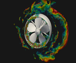
The instantaneous flow field of a ducted propeller in crashback at  $J=-0.82$. An iso-contour of pressure $p=-0.75$ coloured by axial velocity $U_x$. This reveals the irregularly shaped vortex ring as it is shedding, increasing propeller and duct loads. The axial velocity is normalized with $U$ and the pressure is normalized with $\rho$ $U^2$, where $\rho$ is the fluid density.

Extensive work has been performed to characterize and understand the flow physics of crashback for an open propeller. In this configuration, the propeller and its hub are placed in a uniform free stream. Open propeller experiments by Reference Jiang, Dong, Lui and ChangJiang, Dong, Lui, and Chang (Reference Jiang, Dong, Lui and Chang1997) and Reference Jessup, Chesnakas, Fry, Donnelly, Black and ParkJessup et al. (Reference Jessup, Chesnakas, Fry, Donnelly, Black and Park2004), Reference Jessup, Chesnakas, Fry and DonnellyJessup, Chesnakas, Fry, and Donnelly (Reference Jessup, Chesnakas, Fry and Donnelly2006) for propeller David Taylor model basin (DTMB) 4381 used particle image velocimetry (PIV) and laser Doppler velocimetry to identify the main flow features, and measured the loads at numerous advance ratios  $J$ where
 \begin{equation} J = \frac{U}{nD}, \end{equation}
characterizes the relative strengths of the free-stream velocity  $U$ and propeller rotation $n=\omega /2{\rm \pi}$, where $\omega$ is the rotational velocity, and $D$ is the propeller diameter. The use of traditional Reynolds-averaged Navier–Stokes approaches to study crashback are limited due to the unsteady flow characteristics (Reference Chen and SternChen & Stern, 1999; Reference Davoudzadeh, Taylor, Zierke, Dreyer, McDonald and WhitfieldDavoudzadeh et al., 1997). Hybrid methods, detached-eddy simulation and delayed detached-eddy simulation have been used as an alternative (Reference Pergande, Wang, Neitzel-Petersen and Abdel-MaksoudPergande, Wang, Neitzel-Petersen, & Abdel-Maksoud, 2017; Reference Pontarelli, Martin and CarricaPontarelli, Martin, & Carrica, 2017). Large-eddy simulation (LES) has shown to be a good alternative, characterizing in detail the main flow features, flow physics and the unsteady load responses in crashback (Reference Chang, Ebert, Young, Liu, Mahesh, Jang and ShearerChang et al., 2008; Reference Jang and MaheshJang & Mahesh, 2013; Reference Verma, Jang and MaheshVerma, Jang, & Mahesh, 2012; Reference Vyšohlid and MaheshVyšohlid & Mahesh, 2006). Blade leading-edge and trailing-edge separation were identified as the main mechanisms for unsteadiness and high side-force loads, and the stability of the vortex ring was linked to these mechanisms.
A ducted propeller is one where a duct is fitted around the rotor blades (figure 2 $d$). Ducts are commonly used to increase thrust and improve propeller efficiency, to reduce cavitation effects, and to reduce underwater noise. In some cases, the duct acts as a physical barrier to protect the propeller from damage. Although there are a plethora of studies on the effects of the duct in the forward or design mode of operation, less is known about off-design conditions like crashback. For a ducted propeller in crashback, a series of experiments studied propeller DTMB 4381 shrouded by a neutrally loaded duct. Reference Jessup, Chesnakas, Fry and DonnellyJessup et al. (Reference Jessup, Chesnakas, Fry and Donnelly2006) found that the duct has a minimal effect on the rotor loads compared with the open case, and that the vortex ring moves outside the duct as seen in figure 1. Later work focused on measuring the unsteady loads on the duct, and concluded that the addition of a duct increases side forces up to three times the magnitude measured in the open configuration (Reference Donnelly, Jessup and EtebariDonnelly, Jessup, & Etebari, 2010; Reference Swithenbank, Jessup and EtebariSwithenbank, Jessup, & Etebari, 2008). Reference Jang and MaheshJang and Mahesh (Reference Jang and Mahesh2008) used LES in a rotating reference frame to study the effect of the duct geometry on the same propeller. Their work confirmed that high side forces arise from the duct surface; however, it did not account for the stator blades used to support the duct in the experiments (figure 2 $d$). The LES of Reference Jang and MaheshJang and Mahesh (Reference Jang and Mahesh2012) used a sliding interface method to include both the duct and stators with the same propeller, matching the exact geometries used in the experiments. The stators were found to add a significant contribution to the torque coefficient $K_Q$. However, these simulations statistically observed only about 18 revolutions, did not compare the mean flow field with the experiments and the 36 in. variable pressure water tunnel (VPWT) geometry was also not included in the simulation. The crashback experiments note potential water tunnel effects due to close proximity of the vortex ring to the VPWT nozzle shear layer, as visualized in figure 2(c). For validation and a better comparison of the simulation with the experiment, it is important to model its presence. In both these previous LES works, it was found that similar mechanisms play a role in the unsteadiness of the loads on the rotor blades as for the open case. In addition, both works identified the presence of tip-leakage flow, a downstream directed flow between the rotor blade tips and duct surface. The physical source was linked to a high pressure gradient between the pressure and suction sides of the blades inside the duct. High pressure fluctuations were observed near the rotor blade tips and on the inner-duct surface right above the tips. This blade–duct interaction was connected to tip-leakage flow and the high side forces observed. Tip-leakage flow has been studied in the forward mode of operation where it interacts with the inflow into the propeller blade passage and forms a tip-leakage vortex (Reference Oweis, Fry, Chesnakas, Jessup and CeccioOweis, Fry, Chesnakas, Jessup & Ceccio, 2006a, Reference Oweis, Fry, Chesnakas, Jessup and Ceccio2006b). However, there is a lack of detailed work on characterizing tip-leakage flow and its effects in the crashback mode of operation.
( $a$) A cross-sectional slice of the computational domain showing dimensions and boundary conditions. All wall surfaces have a no-slip boundary condition except for those on the rotor blades. The 36 in. VPWT geometry is included to best match the experiments. ( $b$) A cross-section showing the mesh configuration and overlap of all four grids. The background grid (in black) which also contains the VPWT walls overlaps the grids around the duct and propeller. ( $c$) Instantaneous axial velocity $U_x$ contour at the constant $y$-plane slice $y = 0$. Note the acceleration of the flow around the vortex ring and the shear layer expansion into the empty section of the VPWT. ( $d$) The geometries of the propeller, duct and stator blades.

In this paper, LES of flow over a ducted marine propeller using an unstructured overset method is performed at an advance ratio of  $J=-0.82$. The use of overset grids provides considerable flexibility compared with solving in a rotating reference frame, or with a sliding interface method. It improves the grid generation process, maintaining good resolution in relevant areas like the rotor blades and duct. In addition, it reduces the overall number of computational cells due to individual localized meshes of high resolution that do not have to expand out towards the far-field. Inclusion of the 36 in. VPWT is straightforward within the overset framework, connecting the mesh to the duct as well as the propeller. To the best of our knowledge, this work is the first utilization of the overset methodology for LES on a ducted propeller in crashback. Over 200 revolutions are simulated to give a clearer picture of the mean flow field. The physical mechanisms responsible for flow structures like the vortex ring and tip-leakage flow are identified. The relationships between the local flows and the resulting unsteady loads are elucidated as well as the mechanism behind the highest side forces. Thus the objectives of the present work are to: (i) assess the ability of LES using an unstructured overset method to predict crashback for a ducted propeller; (ii) study the origins of the unsteady loads on each of the components and their relationship to flow structures like the vortex ring and tip-leakage flow; and (iii) propose the mechanism behind the highest side forces.
2. Simulation Details
In this work, we use an overset grid method to solve the incompressible Navier–Stokes equations with an arbitrary Lagrangian–Eulerian formulation to account for mesh movements while LES models the sub-grid unresolved scales. The simulation uses an overset grid method developed by Reference Horne and MaheshHorne and Mahesh (Reference Horne and Mahesh2019a, Reference Horne and Mahesh2019b). More details of the numerical method can be found in the supplementary material available at https://doi.org/10.1017/flo.2021.18.
The simulation of a ducted propeller in crashback is set up to match experiments (Reference Donnelly, Jessup and EtebariDonnelly et al., 2010; Reference Jessup, Chesnakas, Fry and DonnellyJessup et al., 2006; Reference Swithenbank, Jessup and EtebariSwithenbank et al., 2008) conducted in a 36 in. VPWT where PIV measurements described details of the flow field, and propeller and duct forces were measured using in-hub 6-component dynamometers. A neutrally loaded duct was designed to fit around propeller DTMB 4381, a five-bladed, right-handed propeller with variable pitch, and no skew or rake. The duct was constructed using stereolithography (SLA) plastic with 13 aligned support vanes or stator blades ahead of the duct. At the propeller design advance ratio of  $J = 0.889$, the duct was designed to contribute no additional propulsor loading. More details of the geometry are provided in Reference Jessup, Chesnakas, Fry and DonnellyJessup et al. (Reference Jessup, Chesnakas, Fry and Donnelly2006, Reference Jessup, Chesnakas, Fry, Donnelly, Black and Park2004), and the geometries are visualized in figure 2( $d$). Note that the duct forces measured in the experiments by Reference Donnelly, Jessup and EtebariDonnelly et al. (Reference Donnelly, Jessup and Etebari2010) used an in-hub dynamometer and thus measured the contributions from both the duct geometry as well as the stator blades as a sum. A different in-hub dynamometer was used to measure loads from the rotor blades separately.
As seen in figure 2( $b$), a total of four unstructured grids represent the flow domain. The background grid contains the 36 in. VPWT walls, the inlet and the outlet as well as the upstream portion of the propeller shaft surrounding all the other grids. There are three overset grids around the duct and the propeller. The duct is represented using two grids, an upstream portion containing the stator blades and a downstream portion containing the rest of the duct. All surfaces on these grids have no-slip boundary conditions. Finally, the propeller grid contains the five rotor blades and part of the inner duct. Only this grid is rotated at the rotational velocity $\omega = 2 {\rm \pi}n$. The $v=\omega \times R$ boundary conditions are prescribed on the rotor blades and hub surfaces contained in this grid, and the inner-duct portion is set to a no-slip boundary condition. More information on the size and partitioning of the grids is presented in table 1. The computational domain with boundary conditions is presented in figure 2( $a$) and the mesh configuration showing the overlap and interpolation edges of all the grids can be seen in figure 2( $b$).
$b$).
Details of the four grids, including the number of control volumes and the number of processors used. The background grid is meant to contain all the other grids within it and has the 36 in. VPWT geometry. The propeller grid is the only dynamic one, to represent the propeller rotation.

During the grid generation process, a cylindrical cut is used to remove redundant control volumes on the background grid in the region where the overset grids are located making sure to leave enough overlap for interpolation (figure 2 $b$). The overset grids are also designed to contain enough overlap for interpolation between each other and the background grid. The background, and duct grids contain only hexahedral control volumes and all surfaces have a minimum wall-normal spacing of 0.00083 $D$ with a growth ratio of 1.01. The propeller grid contains a pill box of tetrahedral cells. On the blade surface of this grid, four prism layers are extruded while on the duct surface, four hexahedral layers are extruded all at an initial wall-normal height of 0.00083 $D$ and a growth ratio of 1.01. The tip gap region has an average spacing of 0.0083 $D$.
$D$.
3. Results
The simulation is performed at the advance ratio  $J=-0.82$ at Reynolds number $Re= 561\ 000$. The Reynolds number $Re$ is defined below
 \begin{equation} Re = \frac{UD}{\nu}, \end{equation}
where  $U$ is the free-stream velocity, $D= 12.0 \ in$ is the propeller disk diameter and $\nu$ is the kinematic viscosity. Thrust $T$ is defined as the axial component of the force. The axial component of the moment is the torque $Q$.
$Q$.  $F_H$ and $F_V$ are the horizontal and vertical components of the force whose vector sum yields the total side force $F_T$. Here, $\rho$ is the fluid density. Non-dimensional thrust $K_T$, torque coefficient $K_Q$ and side-force coefficient $K_S$ are defined as
 \begin{equation} K_T = \frac{T}{\rho n^2 D^4}, \quad K_Q = \frac{Q}{\rho n^2 D^5}, \quad K_S = \frac{\sqrt{F_H^2 + F_V^2}}{\rho n^2 D^4}; \end{equation} $\langle K_T \rangle$ represents the mean of the coefficient $K_T$ and $\sigma (K_T)$ the standard deviation.
The computational time step used for this case is  ${\rm \Delta} tU/D = 2.083 \times 10^{-4}$, which corresponds to a propeller rotation of $0.1286^\circ$ per time step. According to Reference Jessup, Chesnakas, Fry, Donnelly, Black and ParkJessup et al.'s (Reference Jessup, Chesnakas, Fry, Donnelly, Black and Park2004) experimental observations, the force coefficients in crashback do not vary with Reynolds number in the range of $4\times 10^5 < Re < 9\times 10^5$. The Reynolds number used in this study, $Re=561\ 000$, is within this range. In the next section, the LES simulation at $J=-0.82$ is compared in detail with the time-averaged PIV data of Reference Jessup, Chesnakas, Fry and DonnellyJessup et al. (Reference Jessup, Chesnakas, Fry and Donnelly2006) at $J=-0.8$.
3.1 Validation
3.1.1 Circumferentially Averaged Flow Field
The time-averaged flow statistics sampled for 234 revolutions from the LES are circumferentially averaged for comparison with the experimental PIV results of Reference Jessup, Chesnakas, Fry and DonnellyJessup et al. (Reference Jessup, Chesnakas, Fry and Donnelly2006) taken in the  $x$–
$x$– $r$ plane. Contours for the axial and radial components of the mean velocity as well as the turbulent kinetic energy (TKE) calculated from the fluctuating components of the aforementioned directions $k_{xr}=\sqrt []{\overline {(u_x ')^2}+ \overline {(u_r ')^2}}$ are compared in figure 3. The contours of axial velocity with velocity streamlines are also compared in figure 4. The experiments were not able to obtain data in the duct and propeller region, thus this region is blanked out. The TKE from the LES results is that resolved on the grid. Although the resolution of the experimental PIV is coarse compared with the LES, good qualitative agreement is observed.
PIV from the VPWT experiment (Reference Jessup, Chesnakas, Fry and DonnellyJessup et al., 2006) compared with the circumferentially averaged flow field of the LES. From VPWT: ( $a$) axial velocity $U_x$, ( $b$) radial velocity $U_r$ and ( $c$) turbulent kinetic energy $k_{xr}=\sqrt []{\overline {(u_x ')^2}+ \overline {(u_r ')^2}}$ using the $x$ and $r$ fluctuating components only. From present LES: ( $d$) axial velocity $U_x$, ( $e$) radial velocity $U_r$ and ( $f$) resolved turbulent kinetic energy $k_{xr}$ using the $x$ and $r$ fluctuating components only. The flow field quantities are normalized with $\rho$ and $U$.
$U$.

Circumferentially averaged flow field of  $U_x$ with streamlines. ( $a$) VPWT experiment (Reference Jessup, Chesnakas, Fry and DonnellyJessup et al., 2006). ( $b$) Present LES. The axial velocity is normalized with $U$.
$U$.

Figures 3( $d$) and 4( $b$) show reverse flow on both inner- and outer-duct surfaces. Inside the duct, reverse flow is strong but weakens closer to the hub surface. There is a strong radially outward flow upstream of the duct (figure 3b,e) as the propeller-induced reverse flow through the stator blades interacts with the free stream. The vortex ring arises from this interaction, forming above the outer duct surface (figure 4a,b). A recirculation zone is also observed upstream of the duct and stator blades (figure 4 $b$). In figure 3(c, f), TKE is high in the regions where the vortex ring is located throughout the flow field history as well as in a region upstream of the duct where the free-stream and radial flows from the inner duct interact. The highest TKE region begins at the sharp leading edge (LE) of the duct and continues along the inner duct, upstream of the rotor blades. This region is important to the overall mechanism for the high side force from the duct and will be discussed in more detail in later sections.
Profiles are extracted from the LES and the experimental contours at nine axial locations, one at the propeller centre ( $x/R=0.0$) and four each upstream and downstream. Figure 5(a,b) compares the profiles of mean axial and radial velocity, which show encouraging agreement. The location of the mean vortex ring centres is compared in table 2, showing good agreement. Overall, the LES captures the flow field for a ducted propeller in crashback well, and compares well with the experiment of Reference Jessup, Chesnakas, Fry and DonnellyJessup et al. (Reference Jessup, Chesnakas, Fry and Donnelly2006).
Profiles of ( $a$)
$a$)  $U_x$ and ( $b$)
$b$)  $U_r$ at axial locations: dashed lines are VPWT experiments (Reference Jessup, Chesnakas, Fry and DonnellyJessup et al., 2006), and the solid lines are the present LES result. The locations are from left to right $x/D=-1.00$, $x/D=-0.75$, $x/D=-0.50$, $x/D=-0.25$, $x/D=0.00$, $x/D=0.25$, $x/D=0.50$, $x/D=0.75$ and $x/D=1.00$. The velocity values are normalized with $U$.
$U$.

The mean vortex ring centre locations for LES at  $J=-0.82$ compared with the experiments at $J=-0.8$. The distances are measured relative to the centre of the propeller.

3.1.2 Unsteady Loads
The massively separated and highly unsteady flow field in crashback at high  $Re$ produces highly unsteady loads on the ducted propeller components. Table 3 compares the LES load statistics with the experimental measurements by Reference Donnelly, Jessup and EtebariDonnelly et al. (Reference Donnelly, Jessup and Etebari2010), and reasonable agreement is obtained. As observed in the experiments, the force coefficients have high standard deviations from their means with instantaneous load measurements fluctuating about the mean up to 3 times the standard deviation. As expected and also confirmed by Reference Donnelly, Jessup and EtebariDonnelly et al. (Reference Donnelly, Jessup and Etebari2010), the total summed $K_T$ is mostly produced from the rotor blades and is similar statistically to the blade contributions in the open propeller configuration. The total summed $K_Q$ has a smaller magnitude due to opposing contributions from the rotor blades and the stator blades, respectively. It is, however, more accurate to view this sum as separate contributions from each of the two components. The rotor blades contribution of $K_Q$ is the torque that needs to be overcome by the propeller drive engine and that of the stator blades would act on the manoeuvring body they are attached to. Here, $K_S$ is mostly produced by the duct, which has a large surface area and experiences the unsteady effects of the vortex ring.
Statistics of unsteady loads where VPWT refers to the measurements from the (Reference Donnelly, Jessup and EtebariDonnelly et al., 2010) experiments at  $J=-0.8$ and LES is the present result at $J=-0.82$. The duct and stator blade contributions were measured with an in-hub dynamometer upstream of the stator blades which constituted the combined forces, details in Reference Donnelly, Jessup and EtebariDonnelly et al. (Reference Donnelly, Jessup and Etebari2010).

3.2 Flow Physics: Vortex Ring, Tip-Leakage Flow
The vortex ring is one of the most prominent flow features of a crashback flow. The propeller-induced reverse flow collides with the forward-moving free stream to form a ring shaped vortex about the propeller disk. The vortex ring formed around a ducted propeller is visualized in figures 1 and 8(a,b) using an iso-contour of pressure. As described by Reference Jang and MaheshJang and Mahesh (Reference Jang and Mahesh2013), at high  $Re$, the vortex ring is highly unstable and irregular in shape. As it breaks down and re-forms, the stability of the vortex ring has direct impact on the flow features around the propeller and duct vicinity. In addition, it has implications on the strength of the free stream versus the reverse flow which affects the local flows in the rotor blade, stator blade and duct passages, impacting the loads on these components.
The addition of the duct geometry has many implications on the flow field that differentiates the ducted case from the open configuration. The vortex ring forms outside the duct as seen in the circumferentially averaged flow in figure 4, increasing the range of its influence radially further outward. For the open configuration case, Reference Jang and MaheshJang and Mahesh (Reference Jang and Mahesh2013) noted that the vortex ring has direct impact on the local flow near the rotor blade tips. During vortex ring shedding events, its centre moves closer to the blade tips, increasing the angle of attack (AOA) of the flow seen by the blade LE. This then increases tip loading and the magnitude of the force coefficients. For the ducted case, the vortex ring centre is now physically disconnected from the rotor blades and does not explicitly affect the flow on the blade tips as noted by Reference Jang and MaheshJang and Mahesh (Reference Jang and Mahesh2013). However, the vortex ring still has a crucial implicit role on high blade loading.
A major effect resulting from the addition of the duct is the so called tip-leakage flow that occurs in the tip gap, the small space between the rotor blade tips and the duct surface. The flow is induced by a pressure gradient between the pressure and suction sides of the rotor blades as illustrated in figure 6. This flow has also been observed in the forward mode of operation where the tip-leakage flow interacts with the inflow into the rotor blades and forms a tip-leakage vortex (Reference Oweis, Fry, Chesnakas, Jessup and CeccioOweis et al., 2006a, Reference Oweis, Fry, Chesnakas, Jessup and Ceccio2006b). In crashback, the pressure and suction sides of the rotor blades switch and so does the direction of the tip-leakage flow which now interacts with the propeller-induced reverse flow (figure 6). In addition, the high pressure gradients created by separation at the rotor blade sharp LE in crashback results in a more prominent tip-leakage flow compared with the forward mode case.
A schematic of tip-leakage flow (TL) for a ducted propeller in the frame of reference of the marine vehicle. ( $a$) The forward mode case, where the pressure difference results in a net tip-leakage flow moving upstream of the rotor blades. ( $b$) The crashback case, where the pressure difference results in a net tip-leakage flow moving downstream of the rotor blades. Note that tip-leakage flow occurs only in the region near rotor blade tips in the small tip gap. The free stream and propeller-induced flows represent their direction outside the duct.

The circumferentially averaged mean pressure field (figure 7 $a$) shows a strong pressure gradient between the pressure and suction sides of the rotor blade with its strength increasing towards the tips. Reference Jang and MaheshJang and Mahesh (Reference Jang and Mahesh2013) showed that there exists a high pressure gradient between the pressure and suction sides along the whole blade with the peak near the rotor blade tips for the open propeller. For the ducted propeller, the effect of the flow on the pressure field around the rotor blades mostly resembles that of the open configuration. However, there is a major difference caused by the addition of the duct geometry. The duct surrounds the propeller and confines the pressure and suction sides preserving a strong pressure gradient along the rotor blade tip gap. This strong gradient, coupled with the small size of the tip gap is the source of a strong tip-leakage flow.
( $a$) The circumferentially averaged mean pressure field showing contours of pressure. There is a large pressure gradient inside the duct, induced by the pressure and suction sides of the blades. A low pressure region representing the vortex ring can be observed outside the duct. A high pressure region upstream of the duct represents the slowing free stream as it interacts with the reverse flow. ( $b$) The circumferentially averaged flow field showing a contour of axial velocity $U_x$ with streamlines. The flow around the duct is mostly attached. There is a stagnation point downstream of the rotor blades and on the duct surface. The free stream is from left to right. The flow field quantities are normalized with $\rho$ and $U$.
$U$.

Tip-leakage flow also affects the local flow field downstream of the rotor blades. It introduces a positive axial component of velocity moving downstream and opposing the propeller-induced reverse flow. As can be seen in the circumferentially averaged contours with streamlines in figure 7( $b$) as well as the contours in figure 9(a,b), this interaction also creates a recirculation zone just downstream of the rotor blades. The recirculation zones are seen to be local to each rotor blade. Instantaneously, the effects of tip-leakage flow create a complex, three-dimensional flow field downstream of the rotor blades. To complicate things more, the rotor blade-local recirculation zones move along with blade rotation as seen in figure 8(c,d), interacting with the duct surface. As will be discussed in the next section, tip-leakage flow and the blade-local recirculation zones play a crucial role in the side-force production from the duct surface.
( $a$,
$a$, $b$) The instantaneous flow field showing iso-contours of pressure $p=-0.70$ coloured by the axial velocity $U_x$. ( $c$,
$c$, $d$) The instantaneous flow field showing iso-contours of pressure $p=-1.25$ coloured by the axial velocity $U_x$. ( $a$,
$a$, $c$) The broken down vortex ring during a shedding event. ( $b$,
$b$, $d$) A more coherent vortex ring. The flow field quantities are normalized with $\rho$ and $U$.
$U$.

As previously mentioned, for the open propeller, the vortex ring directly interacts with the propeller blades, increasing the AOA of the flow interacting with the sharp LE of the propeller blade tips during high loading events (Reference Jang and MaheshJang & Mahesh, 2013). For the ducted case, the vortex ring does not directly interact with the rotor blade tips. Tip-leakage flow is the mechanism observed to have a similar role. A stronger tip-leakage flow results in higher rotor blade tip loading and an increase in the force coefficient magnitudes produced by the rotor blades. In addition, the vortex ring's stability, can be linked to the strength of tip-leakage flow as well as the rotor blade tip loading.
The effects of the blade-local recirculation zones on the local flow field depends on the strength of the tip-leakage flow versus the propeller-induced reverse flow. This means that the stability of the vortex ring also plays an implicit role. An unstable vortex ring results in a break-up of the vortex ring like in figures 8( $a$) and 9( $a$). This directly affects the flow that enters the duct and makes it non-uniform with higher axial positive velocity in some regions and lower in others. In some regions, a stronger forward-moving flow impinges further into the duct and creates a higher pressure region upstream of the rotor blades. A higher forward-moving flow means a more negative $J$ locally and following the trend seen in the experiments by Reference Donnelly, Jessup and EtebariDonnelly et al. (Reference Donnelly, Jessup and Etebari2010), the magnitude of the force coefficients are expected to increase because of this. The higher pressure inside the duct means that the blades located locally in this region would see an increase in the pressure gradient between the pressure and suction sides and thus the strength of the tip-leakage flow and the blade-local recirculation zone (figure 8a,c). Interestingly, observing along the azimuthal direction, tip-leakage flow can be strong enough to have an effect further away from the rotor blade tips and in between them (figure 8 $c$). Overall, the individual blades rotate in and out of high pressure regions leading to fluctuations in the strength of tip-leakage flow and blade-local recirculation zones with implications on the loads as well.
( $a$) A contour of instantaneous axial velocity $U_x$ at the constant $z$-plane slice $z = 0$ with streamlines of the axial $U_x$ and radial $U_r$ components of velocity. An unstable and broken down vortex ring also seen in figure 8( $a$). This leads to non-uniformity around the duct geometry and an increase in the strength of tip-leakage flow as well as LE separation. The effect is a considerable increase in side-force production from the duct. ( $b$) A contour of instantaneous axial velocity $U_x$ at the constant $z$-plane slice $z = 0$ with streamlines. A stable vortex ring also seen in figure 8( $b$). This leads to a more uniform flow around the duct geometry and lower side forces. The centre of the vortex ring is also close to the average location of ( $x/R=0.65$) and ( $r/R=1.80$). All velocity quantities are normalized with $U$.
$U$.

3.3 Origin of Unsteady Loads
As noted by Reference Chang, Ebert, Young, Liu, Mahesh, Jang and ShearerChang et al. (Reference Chang, Ebert, Young, Liu, Mahesh, Jang and Shearer2008), Reference Verma, Jang and MaheshVerma et al. (Reference Verma, Jang and Mahesh2012), Reference Jang and MaheshJang and Mahesh (Reference Jang and Mahesh2013), the propeller loads in crashback are pressure-driven with separation resulting in highly unsteady loads that fluctuate about their mean. This can result in extreme magnitudes of the loads that occur in low frequency and are almost unpredictable. Understanding the loads in crashback is essential for design aspects. It is also crucial to understand the extreme magnitudes of the side forces due to their relevance to manoeuvring.
3.3.1 Rotor Blades
Similar to the open propeller, the rotor blades are the main source of the negative thrust  $K_T$ and torque $K_Q$ coefficients. These two force coefficients are produced from the pressure difference between the pressure and suction sides of the rotor blades. The largest pressure difference occurs near the sharp LE along the whole rotor blade, pointing to large flow separation here as the mechanism behind the high magnitude of the generated $K_T$ and $K_Q$, similar to what was observed by Reference Verma, Jang and MaheshVerma et al. (Reference Verma, Jang and Mahesh2012), Reference Jang and MaheshJang and Mahesh (Reference Jang and Mahesh2013). Figure 10( $a$) illustrates the distribution of $\langle K_T \rangle$ on blade sections. Not shown, $\langle K_Q \rangle$ closely follows this trend. The highest local contribution to $K_T$ occurs near the rotor blade tips where there is the highest pressure gradient, as seen in figure 7( $a$). Figure 10( $b$) illustrates the distribution of $\langle K_T \rangle$ on blade sections per unit area which also confirms this trend. Instantaneously, these force coefficients have high standard deviations (table 3) and can deviate up to 3 times the standard deviation about the mean as noted by Reference Chang, Ebert, Young, Liu, Mahesh, Jang and ShearerChang et al. (Reference Chang, Ebert, Young, Liu, Mahesh, Jang and Shearer2008), Reference Verma, Jang and MaheshVerma et al. (Reference Verma, Jang and Mahesh2012) and Reference Jang and MaheshJang and Mahesh (Reference Jang and Mahesh2013). The source for this behaviour is the LE separation on the sharp LE of the rotor blades.
( $a$) Radial distribution of mean thrust coefficient $\langle K_T \rangle$, ( $b$) mean thrust coefficient per unit area, ( $c$) mean side-force coefficient $\langle K_S \rangle$ and ( $d$) mean side-force coefficient per unit area all on 10 equal segments along the rotor blades. The $x$-axis is the rotor blade radius normalized by the total radial length of the rotor blade from the hub surface to the tip, $L_R=4.8\ in$.

The LE separation also helps produce a high side-force coefficient  $K_S$ which measures the magnitude of the vertical and horizontal components of the loads. The rotor blade contribution to the mean side-force coefficient $\langle K_S \rangle$ has a peak near the root and another near the tip where it has the highest magnitude (figure 10 $c$). This trend remains the same when looking at $\langle K_S \rangle$ per unit area in figure 10( $d$) with both the root and tip producing almost similar magnitudes. In previous publications on crashback flow for the open propeller (Reference Jang and MaheshJang & Mahesh, 2013; Reference Verma, Jang and MaheshVerma et al., 2012), the largest magnitudes of $K_S$ were found to originate from the blade roots, where there is stronger forward-moving flow that impinges into the blade passage interacting with the reverse flow and forming both LE and trailing-edge separation zones. This mechanism is also observed for the ducted case and is responsible for the significant contribution to $K_S$ from the rotor blade roots. Differing from the open case, there is a high contribution of $K_S$ near the rotor blade tips. For the ducted case, tip-leakage flow is the main driver to increasing the magnitude of $K_S$ in this region. As tip-leakage flow moves downstream, it increases the local AOA seen by the LE of the blade section, simultaneously increasing LE separation and flow unsteadiness. Both these effects on high $K_S$ production are expected to grow following an increase in the magnitude of advance ratio $J$, a trend seen in the experiments by Reference Donnelly, Jessup and EtebariDonnelly et al. (Reference Donnelly, Jessup and Etebari2010).
Compared with the open case, the addition of the duct geometry has a minor effect on the general trends observed on the force coefficients produced from the propeller blades. This was noted by previous experiments as well, (Reference Donnelly, Jessup and EtebariDonnelly et al., 2010; Reference Jessup, Chesnakas, Fry and DonnellyJessup et al., 2006; Reference Swithenbank, Jessup and EtebariSwithenbank et al., 2008). However, analysis of the mean flow field and load distributions shows that the mechanisms behind the force production from the rotor blades are altered with the additional effect of tip-leakage flow.
3.3.2 Stator Blades
The stator blades are used to connect the duct geometry to the hub. They have an airfoil cross-section in order to regularize the flow approaching the rotor blades in forward mode of operation. In crashback, however, they have major effects on the flow field and impact the loads. To study this, we can isolate the loads produced on the stator blades as well as observe the mean flow on their surface and surrounding region. The reverse flow has a component in the negative azimuthal direction due to propeller rotation and collides with the pressure side of the stator blades. The thrust coefficient  $K_T$ is produced by the axial pressure difference created by the strong reverse flow and is therefore net positive, opposite that from the rotor blades. However, its magnitude is negligible overall at only approximately 2 % of that produced by the rotor blades (table 3).
The stator blades produce an appreciable amount of the torque coefficient  $K_Q$ with a magnitude of approximately 70 % that from the rotor blades (table 3). The LE separation is the main mechanism behind this as the propeller-induced reverse flow collides with the sharp LE of the stator blades. The pressure gradient between the pressure and suction sides creates a resultant force in the negative azimuthal direction. This force adds up on all the 13 stator blades producing a net positive $K_Q$, opposite to that produced by the rotor blades (table 3). Figure 11(a) illustrates the distribution of $\langle K_Q \rangle$ on the stator blade sections. The magnitude increases almost linearly from the root following the increasing lever arm. The increase in strength in the reverse flow from the root toward the duct surface is also a contributor to this increase in $K_Q$. It is important to note that, although the direction of $K_Q$ opposes that from the rotor blades, its effects are solely on the manoeuvring vehicle as the $K_Q$ from the rotor blades is counteracted by the propeller engine drive.
( $a$) Radial distribution of mean torque coefficient $\langle K_Q \rangle$ and ( $b$) mean side-force coefficient $\langle K_S \rangle$ on 10 equal segments along the stator blades. The $x$-axis is the stator blade radius normalized by the radial length of the stator blade from the hub surface to the duct, $L_S=4.465\ in$.

The magnitude of  $\langle K_S \rangle$ produced by the stator blades (table 3) is close to that produced by the propeller blades, although it does not necessarily act in the same direction instantaneously. Figure 11( $b$) illustrates the distribution of $\langle K_S \rangle$ on the stator blade sections. The magnitude of $K_S$ increases moving from the root and towards the duct surface. The mechanism behind side-force production is the unsteady flow effects of LE separation. This leads to an almost steady $K_S$ production throughout the stator blade surface.
3.3.3 Duct
The statistics of the force coefficients produced by the duct are shown in table 3. The thrust coefficient  $K_T$ produced by the duct has a relatively small magnitude at approximately 10 % of that produced by the rotor blades. It is negative, acting in the same direction as that produced from the rotor blades, a resultant of the overall pressure field around the duct (figure 7 $a$). The torque coefficient $K_Q$ produced has a negligible magnitude due to the duct surface orientation. These results are consistent with the experiments (Reference Donnelly, Jessup and EtebariDonnelly et al., 2010) as well as previous simulations (Reference Jang and MaheshJang & Mahesh, 2008, Reference Jang and Mahesh2012).
The duct is the main source of the side-force  $K_S$ production. The main reason that its magnitude can get so high is the large surface area on the duct available for pressure forces to act on. In addition, the instantaneously complex and highly varying pressure field around the duct geometry creates situations where large magnitudes of $K_S$ are possible. Observing the circumferentially averaged mean pressure field in figure 7( $a$), the vortex ring creates a low pressure region outside the duct surface. Inside the duct, forward-moving flow creates a high pressure region upstream of the rotor blades while LE separation creates a low pressure region downstream of them. Due to the symmetry of the duct geometry, a side force only occurs due to non-uniformities in the flow field that affect the pressure field inside and outside it. There are three identified flow features around the duct geometry that can cause this and are thus the mechanisms for high $K_S$ on the duct. These are the vortex ring, the blade-local recirculation zones caused by tip-leakage flow and LE separation on the sharp LE downstream of the duct.
Figure 12 illustrates the distribution of the mean side force  $\langle K_S \rangle$ on the duct sections from upstream to downstream. Moving from left to right, the total production of $K_S$ is minimal on the upstream part of the duct followed by a slight increase and a steady amount throughout the duct with an increase after the rotor blade passage, and finally a pinnacle at the sharp LE downstream. This observed distribution can be related to the flow field features. Due to the vortex ring, the pressure field in the outer duct contributes a steady amount of $K_S$ throughout as seen in figure 12. The inner duct distribution shows a lower $K_S$ contribution upstream of the rotor blades where the reverse flow is strongest and TKE is lower as seen in figure 3( $\,f$). Surprisingly, unsteadiness introduced by LE separation from the stator blades near the duct surface is not enough to make an appreciable impact. Overall, the vortex ring globally contributes to a total high $K_S$ magnitude on the duct.
Axial distribution of mean side force  $\langle K_S \rangle$ on 10 equal segments along the duct: inner $\triangle$; outer $\diamond$; total $\circ$. The $x$-axis is normalized by the axial length of the duct $L_D=10.043\ in$, going from upstream (left) to downstream (right). The rotor blade is located at approximately $x/L_D = 0.6$.

The rest of the mechanisms are local to certain areas on the duct and have an impact on the fluctuation in  $K_S$ produced mostly by the vortex ring. First, the effects of the rotor blades on $K_S$ are evident in figure 12. Upstream of the rotor blade passage ( $x/L_D=0.6$), there is an increase in total $K_S$ caused by an increase in the inner duct. This is followed by a slight drop downstream. This confirms a blade–duct interaction caused by the physical presence of the rotor blades as they rotate. More specifically, this is the effect of blade-local recirculation zones caused by tip-leakage flow, as they rotate with the propeller blades. We also see an increase in $K_S$ the farther we move downstream in figure 12 as the region of influence of the blade-local recirculation zones extends further downstream as seen in figures 7( $b$) and 9(a,b).
However, this by itself is not enough to produce the largest local side forces. Further downstream, there is an even larger increase in total  $K_S$ caused by an increase in the inner-duct contribution. The LE separation on the sharp duct LE, as seen in figure 9(a,b), is the final mechanism for local $K_S$ production. This is the main contributor to the highest local $K_S$, produced on the downstream most section of the duct (figure 12). Very much similar to the other components, this mechanism is dependent of the strength of the reverse flow.
Instantaneously, the overall magnitude of  $K_S$ can increase up to 3 standard deviations above the mean. The largest of these fluctuations are unpredictable and occur at low frequencies. The cause of this can be linked to the break-up and re-formation of the vortex ring, figure 8(a,c). The vortex ring break-up creates a pressure field that loses symmetry resulting in a net $K_S$. Due to the scale of the vortex ring and the large surface area it influences on the duct, it has the largest effect on the overall large magnitude of $K_S$. The LE separation increased by the higher reverse flow on certain sections of a broken down vortex ring contributes a significant amount of local $K_S$ to this total. The large local $K_S$ caused by tip-leakage flow and the blade-local recirculation zones contribute as well. When the vortex ring is more stable, figure 8(b,d), LE separation contributes to the highest of $K_S$ locally, and the blade-local recirculation zones play a more important role leading to high fluctuations in total $K_S$ on the duct. However, the total side force produced is lower in magnitude compared with a state where the vortex ring is broken down. The contours in figure 9(a,b) summarizes the effects of a stable and unstable vortex ring on the side forces.
4. Summary
A novel unstructured overset methodology is applied to simulate the flow over a ducted propeller in crashback under the same conditions as experiments, comparing well. To the best of our knowledge, these simulations are the first that reproduce detailed velocity profiles observed in experiment and are also the first application of an unstructured overset methodology to perform LES of the ducted crashback problem. There is little work and detailed description of the crashback mode of operation for a ducted propeller and how it differs from the open configuration. This work helps create a more clear, general description of the flow field as well as the unsteady loads. Comparing the ducted propeller with the open configuration, the mechanisms behind the unsteady force coefficients on the rotor blades are similar, LE separation identified as being primary. One difference is that the vortex ring does not directly impact the local flow near the rotor blade tips. Tip-leakage flow takes its place leading to high rotor blade tip loading. The largest difference between the two configurations, however, is the higher side-force production due to the effects of the addition of the duct geometry.
Observations of the flow reveal the propeller-induced reverse flow interacts with the free-stream velocity to form the globally prominent vortex ring outside the duct. The vortex ring is responsible for a high total  $K_S$ production on the duct surface due to its effect on the pressure field. As the vortex ring breaks up, it leads to non-uniform flow around the duct creating a large magnitude side force. To mitigate its effects on manoeuvring, it is important to consider the overall duct surface area during the design process.
The vortex ring is also found to have an influence on the local flows in the different components, as the duct, rotor blades and stator blades experience the effects of LE separation on their sharp LE. The strength of this separation is dependent on the strength of the propeller-induced reverse flow which is linked to the vortex ring and its stability. This mechanism results in high fluctuations of  $K_T$ and $K_Q$ on the rotor and stator blades and also $K_S$ production on all components, with the largest values on the duct. The largest $K_S$ fluctuations caused by LE separation on the duct could be reduced by weakening the strength of the reverse flow that approaches it.
The rotor blades coupled with the duct geometry produce tip-leakage flow, whose effects on the local rotor blade and inner-duct flow field are described. All force coefficient magnitudes on the rotor blades increase with its strength which is linked to the stability of the vortex ring in that an unstable vortex ring leads to non-uniform flow with a local increase in tip-leakage flow where forward-moving flow is stronger. Due to the high pressure gradients inside the duct in crashback, the strength of tip-leakage flow is more significant compared with that in forward mode. It results in blade-local recirculation zones that affect the flow field downstream of the rotor blades as they fluctuate in strength, moving upstream and downstream along the duct surface. In addition, they rotate with the rotor blades, their strengths varying with the local flow and pressure field they experience. Overall, these blade-local recirculation zones lead to fluctuations of local  $K_S$ and an increase in total $K_S$ production on the duct.
Acknowledgements
The authors would like to thank Dr W. Horne and N. Morse for their thoughtful comments and discussion throughout this work.
Funding Statement
This work was supported by the United States Office of Naval Research (ONR) under ONR grant N00014-18-1-2356 with Dr K.-H. Kim as grant monitor. Computational resources were provided by the U.S. Army Engineer Research and Development Center (ERDC) in Vicksburg, Mississippi on the Cray XC40/50, Onyx of High Performance Computing Modernization Program (HPCMP) and the Minnesota Supercomputing Institute (MSI) at the University of Minnesota.
Declaration of Interests
The authors declare no conflict of interest.
Author Contributions
T.B.K. created the grids, ran the simulations and post-processed the data. T.B.K and K.M. wrote the manuscript.
Data Availability Statement
Raw data will not be available.
Ethical Standards
The research meets all ethical guidelines, including adherence to the legal requirements of the study country.
Supplementary Material
Supplementary material are available at https://doi.org/10.1017/flo.2021.18.


 Open access