

1.1 Introduction
The science of spectroscopy dates back to the seventeenth century with Newton’s demonstration of the dispersion of sunlight into a spectrum of colours, but it was not until the nineteenth century that it was recognised that elements and molecules possess a characteristic emission or absorption spectrum. Observation of emission or absorption line spectra became an important method for the identification of chemical compounds and the only method for determining the composition of stars and other objects in our universe. The advent of the laser in the second half of the twentieth century marked the era of modern spectroscopy, opening up new techniques based on the laser’s unique properties of high intensity, spectral purity and coherence. Additionally, over the past 30 years the widespread deployment of fibre optic data communication has led to the ready availability of low cost and versatile laser sources in the near-IR region of the spectrum, as well as low-loss fibres and a variety of fibre components. Today, laser absorption spectroscopy in the near-IR and mid-IR spectral regions is a well-established technique for the identification of gases and for the measurement of gas parameters such as concentration, pressure and temperature. The primary focus of this book is on near-IR gas absorption spectroscopy to take advantage of the maturity of near-IR lasers and photonics, but it should be noted that the principles and methods discussed throughout are equally applicable to the longer wavelength mid-IR region, which will be considered in detail in Chapter 8. In this chapter we will review the fundamental principles and parameters used to describe the absorption spectroscopy of gases, covering topics such as the Beer–Lambert law, lineshapes and line-broadening mechanisms, fundamental and overtone absorption lines and the measurement of gas parameters from lineshape information.
1.2 Fundamentals of Optical Absorption
1.2.1 Definition of Parameters
There are several parameters used to describe the absorption of light by gas molecules. We start with the definition of the absorption cross-section for a single gas molecule, where the molecule is viewed as having an effective area, σ, for the capture or absorption of a photon from a beam of intensity, I(x,y), as shown in Figure 1.1.
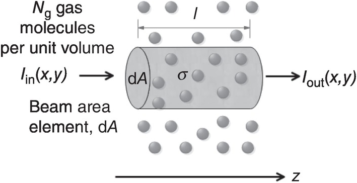
Figure 1.1 Description of the parameters used in the Beer–Lambert law.
Considering a cross-sectional area of dA = dxdy , the probability of photon capture or absorption by the molecule is σ/dA. Over a short length, dz, in the propagation direction, the beam will encounter NgdAdz gas molecules and the rate of photon absorption or change in beam intensity will therefore be:
 (1.1)
(1.1)where Ng is the number density of the target gas molecules (number per unit volume) and we assume that this density is uniform in the (x,y) transverse plane and along beam direction, z.
The power in the beam is P = ∬ I(x, y)dxdy and hence integration of (1.1) leads to the Beer–Lambert law for the transmitted power, Pout, after a path length, l, over which the beam and gas interact:
where Pin is the incident beam power.
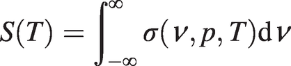
As shown in Figure 1.2, the absorption cross-section, σ, is dependent on the optical frequency, ν, gas pressure, p, and temperature, T, and may be written as σ(ν, p, T) = S(T)ϕ(ν, p, T), where ϕ(ν, p, T) describes the lineshape function and S is the line strength per molecule defined by:
 (1.3)
(1.3)Note that with the above definitions, ϕ(ν, p, T) is normalised so that  .
.
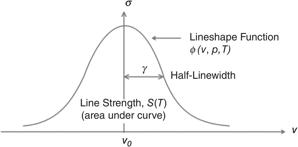
Figure 1.2 Typical absorption cross-section of a gas molecule and the associated parameters.
The number density, Ng, in (1.2) may be expressed in terms of the mole fraction or partial pressure of the target gas using the ideal gas law and Dalton’s law:
 (1.4)
(1.4)where n is the total number of moles and ni and pi are the number of moles and the partial pressure of each of the constituent gases, respectively.
Hence we can write for the number density of the target gas:
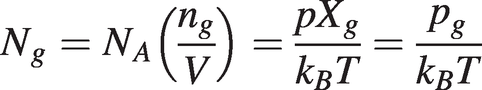 (1.5)
(1.5)where NA is Avogadro’s number, kB = R/NA is the Boltzmann constant, p is the total gas pressure, ng is the number of moles, pg the partial pressure and Xg = ng/n is the mole fraction of the target gas.
Hence the Beer–Lambert law may be written as:
where S′(T) = S(T)/(kBT).
Another commonly used parameter is the absorption coefficient, α, where the absorption cross-section or line strength for a single molecule is multiplied by N0 as follows:
where N0 = p0/(kBT0) ≅ 2.5 × 1025m−3 is the molecular density at normal temperature and pressure (NTP, T0 = 293.15 K, p0 = 1 atm pressure or 101.325 kPa).
The Beer–Lambert law is then:
where the target gas concentration is given by C = Ng/N0 = (T0/T)(pXg/p0) = (T0/T)(pg/p0), with T0 = 293.15 K and p0 = 1atm pressure.
Equations (1.2), (1.6) and (1.8) represent useful equivalent forms of the Beer–Lambert law for calculating the gas absorption.
1.2.2 Absorption Lineshape Functions
The absorption lineshape function, ϕ(ν, p, T), for gases is determined by three line-broadening mechanisms, namely, natural (or lifetime) broadening, Doppler broadening and collisional (or pressure) broadening [Reference Demtroder1, Reference Fox2].
1.2.2.1 Natural Broadening
Photon absorption occurs when an electron, atom or molecule is raised from a lower to a higher energy level. However, in accordance with the uncertainty principle, ΔEΔt ≥ h, the levels have an uncertainty in their energy giving rise to a small range of optical frequencies over which the absorption occurs. Similar to the exponential decay in spontaneous emission of light from downward transitions, which is characterised by a Lorentzian function in the frequency domain, the absorption lineshape from natural broadening is also described by a normalised Lorentzian function with a natural half-linewidth, γn. Natural broadening represents the limit in the sharpness of a spectral line, but will not be considered further here since for most practical applications the linewidth is dominated by Doppler or pressure-broadening effects, as discussed below.
1.2.2.2 Doppler Broadening
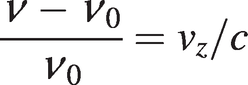
The random thermal motion of gas molecules means that the optical frequency ‘seen’ by a molecule is shifted due to the Doppler effect. The frequency shift will be positive or negative depending on whether the z-component of the molecular velocity, νz, is in the opposite or in the same direction as the beam propagation along the z-axis (the velocity component perpendicular to the beam will have no effect). The frequency shift is given by:
 (1.9)
(1.9)where ν0 is the centre frequency of the transition.
The number of gas molecules with a velocity component between νz and νz + dνz is given by the one-dimensional Maxwell–Boltzmann distribution:
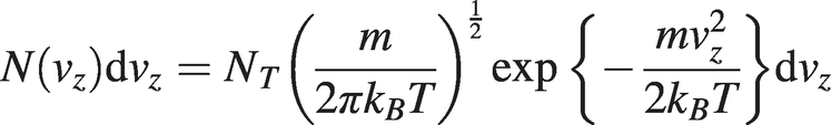 (1.10)
where NT is the total number of molecules and m is the molecular mass.
Substituting vz = (c/ν0)(ν − ν0) and dvz = (c/ν0)dν from (1.9) into (1.10) and, since the absorbed power in the range ν to ν + dν will be proportional to the number of molecules in the range νz to νz + dνz, we obtain a normalised Gaussian lineshape for Doppler broadening as:
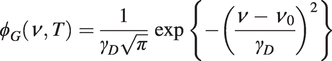 (1.11)
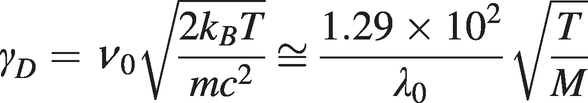 (1.12)
where M is the molecular weight in atomic mass units. The half-width-half-maximum linewidth is  . Typically, for CO2 at an absorption wavelength of ~2 µm, with M = 44 and T ~300 K, γHWHM ~ 0.14 GHz.
1.2.2.3 Collisional Broadening
Gas molecules are subject to random collisions and, as the molecules approach each other during collisions, their energy levels will be perturbed, each level by differing amounts. Hence the frequency of photon absorption during a collision will differ from the unperturbed situation, resulting in collisional broadening of the absorption line. From a simple analysis, we would expect the line broadening to be dependent on the collision rate or inversely on the mean time, τc, between collisions. In turn, the collision rate will be proportional to the collision cross-section, σc, the total number density of molecules present, ND = p/kBT (from the ideal gas law) and the average molecular speed,  (from the Maxwell–Boltzmann distribution). Hence:
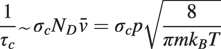 (1.13)
Collisional (or pressure) broadening produces a normalised Lorentzian lineshape of the form:
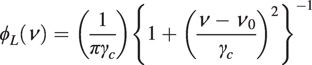 (1.14)
where, from (1.13), the half-linewidth will have a pressure and temperature dependence of the form:
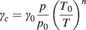 (1.15)
where γ0 is the half-linewidth at NTP and the temperature index, n, is ½ in the simple model outlined above, but in practice may differ from this value.
Broadening will, however, depend on whether collisions occur between molecules of the same species (self-broadening by the target gas) or cross-broadening from different species. The overall broadening may be approximated as the weighted sum of self-broadening and cross-broadening effects. For example, for the target gas in air:
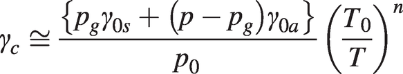 (1.16)
where γ0s and γ0a are the self- and air-broadened half-widths at NTP and pg is the partial pressure of the target gas.
Note from the above discussion that the Doppler linewidth is dependent only on temperature, whereas pressure broadening depends on pressure and inversely on temperature. At NTP, pressure-broadened linewidths are typically of the order of several GHz and dominate over Doppler broadening. However, at lower pressures and/or higher temperatures where the pressure and Doppler-broadened linewidths are comparable, the lineshape may be described by a convolution of the normalised Gaussian and Lorentzian lineshapes:
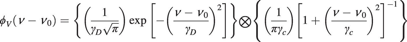 (1.17)
This convolution function is also normalised and may be written as:
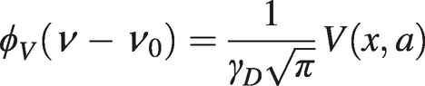 (1.18)
where V(x, a) is the Voigt function [Reference Voigt3] defined by the integral:
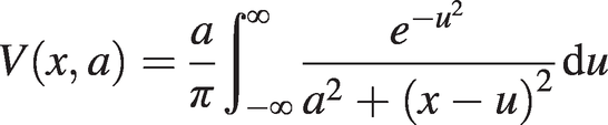 (1.19)
with x = (ν − ν0)⁄γD , a = γc⁄γD.
The Voigt function cannot be evaluated analytically, but various approximations are given in the literature [Reference Drayson4–Reference Huang and Yung7]. Approximations to the Voigt linewidth are discussed by Olivero and Longbothum [Reference Olivero and Longbothum5].
1.3 Extraction of Gas Parameters from Absorption Line Measurements
Measurement of the half-width, γ, and line centre depth, dc, of an absorption line yields information on the gas concentration, pressure or temperature. In situations where Doppler broadening is dominant, the target gas temperature may be determined uniquely from the linewidth using (1.12). The normalised depth of a Doppler-broadened line from (1.6) and (1.11) is:
 (1.20)
which gives  and the approximation applies for small absorbance.
Hence knowing the line strength and gas cell length, the partial pressure (or target gas concentration) may be determined from the measured line depth and width, but no information can be gained on the total gas pressure if other gases are present.
Where collisional broadening is dominant, the normalised depth of the Lorentzian profile from (1.6) and (1.14) is:
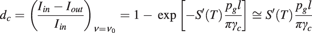 (1.21)
which gives pg ≅ (πγcdc)⁄{S′(T)l}.
So again the partial pressure (or target gas concentration) may be determined from the measured line depth and width, knowing the line strength and gas cell length.
However, the linewidth depends on both pressure and temperature for Lorentzian and Voigt profiles, as shown by (1.16), and hence additional information is required to determine both pressure and temperature. For this, we can make use of the fact that the line strength, defined by (1.3) as the area under the absorption cross-section distribution, is a function of temperature only and is not dependent on the linewidth. This is because the broadening mechanisms spread the absorption probability distribution function over a wider range of frequencies, but the total integrated probability remains the same for the same number density of target gas.
Hence if we simultaneously measure the widths (γ1 and γ2) and normalised depths (dc1 and dc2) of two nearby absorption lines of the same species, then, since the gas concentration and cell length are the same for both lines, the ratio of line strengths may be calculated from (1.20) or (1.21) for small absorbance as:
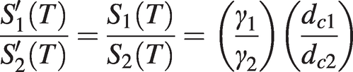 (1. 22)
This ratio of line strengths, which is purely a function of temperature, may be calibrated against temperature for two particular absorption lines and used for gas temperature measurements. (Alternatively for large absorbance, this ratio may be computed from the ratio of areas under the two lines.) For this procedure it is clearly advantageous to choose two lines where the line strength variation with temperature is significantly different; see Arroyo [Reference Arroyo and Hanson8] for more information.
Finally, we note that high-speed gas flows can be monitored from the Doppler effect on the central position of an absorption line. If the absorption line is monitored by two beams, one parallel and one orthogonal to the direction of gas flow, then the shift, Δν0, in the line centre position between the two measurements is simply related to the gas flow velocity, Vg, by: Δν0 = (Vg/c)ν0.
1.4 Absorption Spectra of Gases
Here we briefly review the origin and nature of the absorption lines of gases, with a particular interest in the near-IR region. A more detailed account may be found in references [Reference Hollas9–Reference Barrow12]. In general, absorption lines arise from the excitation of rotational and vibrational states of gas molecules and from electron transitions between orbitals of the atoms involved. As in the case of electronic transitions, the rotational and vibrational states are quantised, giving rise to a discrete set of energy levels and absorption lines. In broad terms, the energy separations of rotational levels correspond to the microwave region, vibrational transitions to the mid-IR region and electronic transitions to the <1 µm wavelength region. However, as we shall see, both rotational and vibrational transitions have an important bearing on the near-IR absorption spectrum. Diatomic molecules possessing two atoms of the same type, such as O2 or H2 undergo no changes in electric dipole moment under rotation or vibration so have no rotational or vibrational spectra and their spectral features of interest arise from electronic transitions.
1.4.1 Rotational Lines of Gases
A molecule may be excited into rotational states through the interaction of the oscillatory electric field of the radiation with the electric dipole moment of the molecule. Hence the existence of a pure rotational line spectrum depends on whether the molecule has a permanent dipole moment. Symmetric linear molecules such as CO2 and highly symmetric spherical molecules such as CH4 have no permanent electric dipole moment and hence no pure rotational line spectrum in the microwave region. However, as discussed below, rotational line spectra for these molecules may appear in combination with vibrational states.
In describing molecular rotation, it is convenient to consider three principal axes of rotation through the centre of gravity of the molecule. A key factor in determining the rotational energy states and hence the rotational line spectrum is the moment of inertia associated with each axis, which in turn depends on the shape and symmetry of the molecule. For diatomic gases such as CO and linear molecules such as CO2 (see Figure 1.3a), the moment of inertia for rotation around the bond axis is approximately zero, while rotation around the other two orthogonal axes has the same moment of inertia so these molecules possess only one series of rotational absorption lines. Highly symmetric spherical molecules such as CH4 have, to a first approximation, the same moment of inertia for all three principal axes so likewise have a single series of rotational lines (although fine structure exists and may be observed at low pressure). Most molecules have three different moments of inertia, e.g. H2O, SO2, NO2, etc., so possess three basic series of rotational line spectra and combination series from rotation about more than one axis.
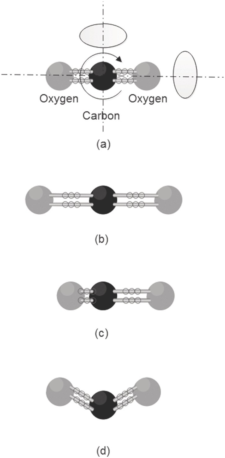
Figure 1.3 Rotation and vibration of the CO2 molecule (a) the three axes of rotation, (b) symmetric stretch mode, (c) anti-symmetric stretch mode, (d) bending mode.
1.4.2 Vibrational Lines of Gases
In a simple model, the bond between the atoms of a molecule may be viewed as a spring obeying Hooke’s law, and the vibrations of a molecule as a mass–spring system forming a simple harmonic oscillator. According to the rules of quantum mechanics, the allowed energy states of the oscillator are quantised according to En = (v + ½)hf0 where f0 is the classical oscillation frequency, v = 0, 1, 2, …, and changes in the vibrational state are restricted to: Δv = ±1. However, the real behaviour of molecular bonds differs from the simple Hooke’s law model and the vibrations are better described as an anharmonic oscillator, as shown in Figure 1.4, with quantised energy states, En = (v + ½)hfa{1 − xa(v + ½)}, where fa is a characteristic frequency and xa is the anharmonicity factor. The spacing between the energy states is no longer uniform and the allowed transitions are governed by the selection rule, Δv = ±1, ±2, ±3, … However, the probability of large jumps is small and at normal temperatures the populations of states with v ≥ 1 is small, so the main vibrational transitions of interest are the fundamental, first and second overtones, corresponding to ν changing from 0 → 1, 0 → 2, 0 → 3, respectively, with diminishing probability and line strength. The fundamental transition 0 → 1 is typically in the mid-IR region for gases, with the near-IR region corresponding to first and second overtones giving absorption lines which are two or more orders of magnitude weaker than the fundamental. Note that at high temperature, transitions from the v = 1 state (known as a vibrational hot-band) may become important.
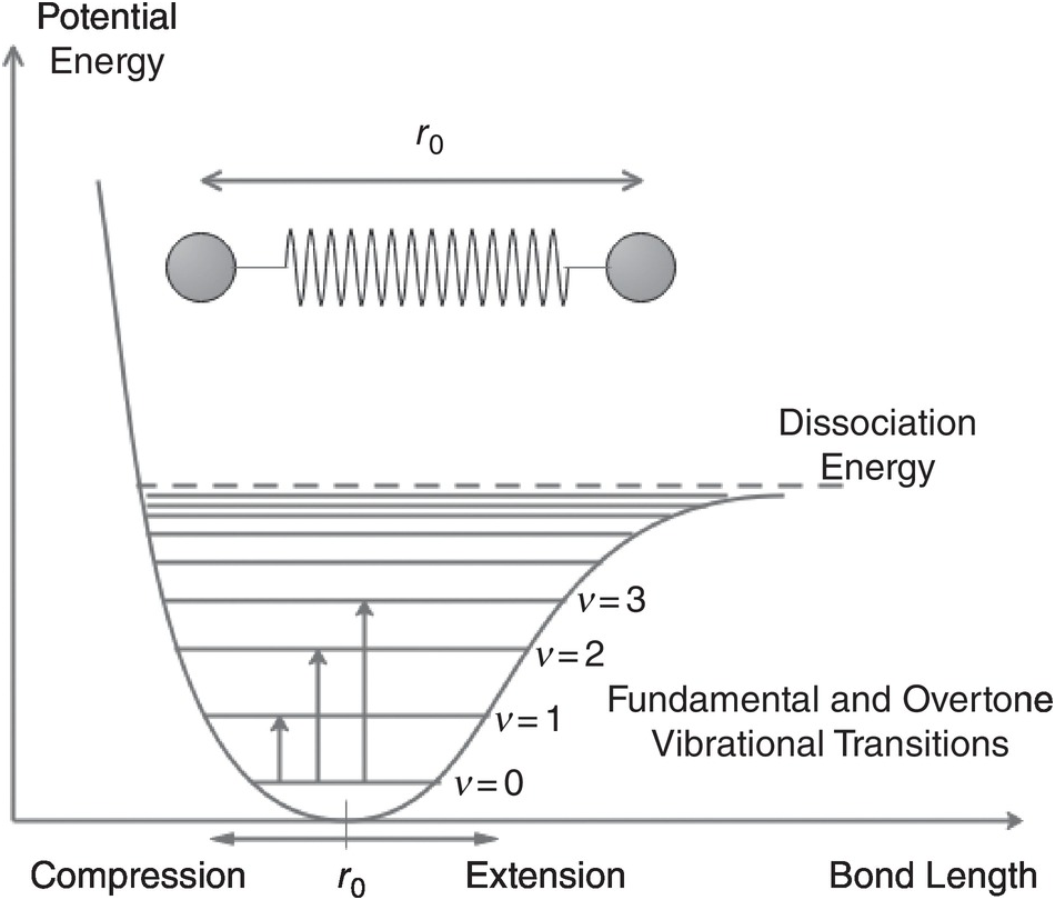
Figure 1.4 The energy levels of the anharmonic oscillator.
The above discussion applies in principle to each vibration mode of a molecule. In general, a molecule containing N atoms can undergo 3N – 6 modes of vibration (3N – 5 for linear molecules). This includes N – 1 bond-stretching motions, with the others being bending motions. Of course, a vibration mode must produce a change in the dipole moment of the molecule for it to interact with the exciting radiation; for example, the symmetric stretching mode of the linear CO2 molecule (see Figure 1.3b) does not give rise to vibrational absorption lines, whereas the anti-symmetric stretching mode (Figure 1.3c) does. Animations of the vibration modes of various molecules, such as methane, may be viewed on the web, see, for example, reference [Reference Greeves13].
As well as pure vibrational modes, a molecule may be excited into a superposition of vibration modes giving vibrational energy levels corresponding to combination and difference bands. For example if ν2 represents the (doubly degenerate) vibration mode of CH4 at ~ 6.5 µm and ν3 represents the (triply degenerate) asymmetric stretching mode ~3.3 µm, then the first overtone, 2ν3, gives rise to near-IR absorption lines around 1.66 µm and the combination, ν2 + 2ν3, gives lines around 1.33 µm (note that IR-inactive vibration modes may appear in combination with other modes). Table 1.1 provides a list of the vibration modes and absorption regions (λ >1 µm) for some common gases.
Table 1.1 Vibrational modes and absorption regions (λ >1 µm) for some common gases
| Gas molecule | Vibrational mode | Wavelength region of absorption lines (µm) |
|---|---|---|
| Carbon monoxide (CO) Linear molecule, N = 2, one stretching mode only, with P and R branches only | Stretching mode, ν1 2ν1 3ν1 | 4.666 2.347 1.575 |
| Carbon dioxide (CO2) Linear molecule, N = 3, four fundamental vibrational modes (two degenerate bending modes) | Symmetric stretch, ν1 | IR inactive |
| 2-degenerate bend, ν2 | 14.986 | |
| Asymmetric stretch, ν3 | 4.257 | |
| 2ν2+ν3 | 2.768 | |
| ν1+ν3 | 2.692 | |
| 4ν2+ν3 | 2.060 | |
| ν1+ 2ν2+ν3 | 2.01 | |
| 2ν1+ν3 | 1.961 | |
| 6ν2+ν3 | 1.646 | |
| ν1+ 4ν2+ν3 | 1.606 | |
| 2ν1+ 2ν2+ν3 | 1.575 | |
| 3ν1+ν3 | 1.538 | |
| 3ν3 | 1.434 | |
| 2ν2+3ν3 | 1.221 | |
| ν1+3ν3 | 1.206 | |
| Methane (CH4) Tetrahedral molecule, N = 5, giving nine vibrational modes but several are degenerate | Symmetric stretch, ν1 | IR inactive |
| 2-degenerate bend, ν2 | 6.523 | |
| 3-degenerate asymmetric stretch, ν3 | 3.312 | |
| 3-degenerate asymmetric bend, ν4 | 7.628 | |
| 2ν 4 | 3.828 | |
| ν2+ν4 | 3.534 | |
| ν2+2ν4 | 2.425 | |
| ν1+ν4 | 2.368 | |
| ν3+ν4 | 2.304 | |
| ν2+ν3 | 2.203 | |
| ν3+2ν4 | 1.791 | |
| ν1+ν2+ν4 | 1.732 | |
| ν2+ν3+ν4 | 1.706 | |
| 2ν 3 | 1.666 | |
| ν2+2ν3 | 1.331 | |
| 2ν1+2ν4 | 1.187 | |
| Water vapour (H2O) Non-linear molecule, N = 3, three fundamental vibrational modes | Symmetric stretch, ν1 | 2.734 |
| Bending mode, ν2 | 6.270 | |
| Asymmetric stretch, ν3 | 2.662 | |
| 2ν2 | 3.173 | |
| 3ν2 | 2.143 | |
| ν1+ν2 | 1.910 | |
| ν2+ν3 | 1.876 | |
| ν1+2ν2 | 1.476 | |
| 2ν2+ν3 | 1.455 | |
| 2ν1 | 1.389 | |
| ν1+ν3 | 1.379 | |
| 2ν3 | 1.343 | |
| ν1+3ν2 | 1.209 | |
| 3ν2+ν3 | 1.194 | |
| 2ν1+ν2 | 1.141 | |
| ν1+ν2+ν3 | 1.135 | |
| ν2+2ν3 | 1.111 | |
| Hydrogen sulfide (H2S) Non-linear molecule of similar shape to water, N = 3, three fundamental vibrational modes | Symmetric stretch, ν1 | 3.726 |
| Bending mode, ν2 | 7.752 | |
| Asymmetric stretch, ν3 | 3.830 | |
| 2ν2 | 4.129 | |
| ν1+ν2 | 2.646 | |
| ν2+ν3 | 2.639 | |
| ν1+ν3 | 1.940 | |
| 2ν1+ν2 | 1.590 | |
| ν1+ν2+ν3 | 1.590 | |
| ν2+2ν3 | 1.565 |
1.4.3 Rovibrational Lines
In general, molecules may simultaneously undergo both vibration and rotation, giving rise to rovibrational energy states. This includes molecules such as CO2, CH4, etc., which have no permanent dipole moment and hence no pure rotational spectra, but undergo dipole changes during vibration. As noted earlier, the energy separation of the vibrational states of a gas molecule is typically in the mid-IR region, whereas for rotational states the energy separation is two or three orders of magnitude smaller, in the microwave region. The large difference in these energies means that, to a first approximation, the total energy of a combined rovibrational state is simply the sum of the separate rotational and vibrational energies. Associated with each vibrational absorption line there is a series of closely spaced rotational lines. For linear molecules where the vibration mode produces dipole changes parallel to the major axis of rotational symmetry (e.g. the anti-symmetric stretching mode of CO2 in Figure 1.3c), transitions between vibrational states must be accompanied by a change in the rotational state, ΔJ = ±1, but for a vibration mode producing perpendicular dipole changes (e.g. the bending mode of N2O), ΔJ = 0, ±1 is allowed. For the vibration modes of non-linear molecules, the selection rules are more complex, but ΔJ = 0, ±1 is often allowed (e.g. the asymmetric stretching mode of CH4). Rovibrational lines corresponding to ΔJ = −1, 0, +1 are described as the P, Q, R branches, respectively. Figure 1.5 illustrates the above principles showing the origin of typical rovibrational absorption lines in the near-IR with the P, Q and R branches.
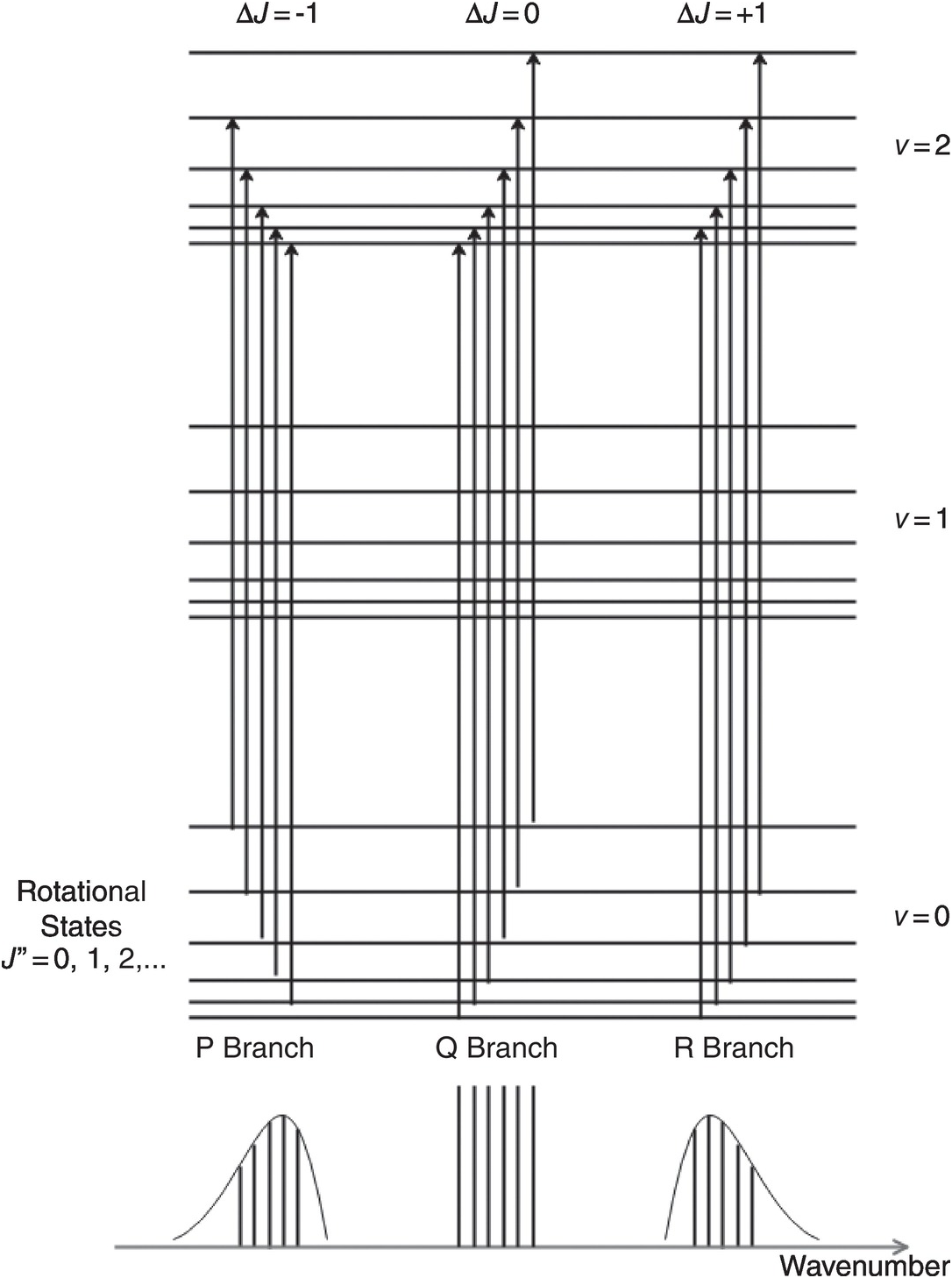
Figure 1.5 Characteristics of typical rovibrational absorption lines in the near-IR showing the P, Q and R branches.
1.4.4 Examples of Gas Absorption Spectra
An extremely useful source of information on spectral line parameters of atmospheric gases and pollutants is the HITRAN database [Reference Gordon, Rothman and Hill14, Reference Rothman15] which also includes an extensive list of references. The HITRAN Application Programming Interface (HAPI) [Reference Kochanov, Gordon and Rothman16, Reference Kochanov, Gordon and Rothman17] and HITRAN on the Web Reference Rothman[18] may be used for the modelling of absorption spectra, including plotting absorption coefficients, and absorption and transmission functions for a variety of important gases and mixtures, with various adjustable parameters such as temperature, pressure, lineshape (Voigt, Lorentz or Doppler), path length, wavenumber range, etc. Outputs are provided in graphical or tabular form which may be downloaded for processing by EXCEL or other programmes.
Figures 1.6–1.12 show some of the stronger near-IR absorption lines for several common and important gases plotted using HITRAN on the Web Reference Rothman[18] with a concentration length product of Cl = 1 cm in (1.8). For comparison, the mid-IR absorption lines for CO, CO2 and CH4 with a much smaller value of Cl = 0.01 cm are shown in Figure 8.1 in Chapter 8, clearly showing the relatively weak strength of the near-IR lines. Note that for our purposes we have plotted the spectra in terms of wavelength (µm) rather than the commonly used wavenumber (cm–1) and hence the order of the P, Q and R branches is reversed. The transmittance (T) on the vertical axis corresponds to the ratio, Pout/Pin, as defined by (1.2), (1.6) or (1.8). Note that the vertical scale differs between graphs to clearly show the line depths. All the examples of the near-IR spectra shown in Figures 1.6–1.12 are for the most abundant isotopologue of the pure gas at a pressure of 1 atm, temperature of 296 K and an absorption path length of 1 cm (hence Cl = 1 cm) with the assumption of a Voigt profile for the lineshape function.
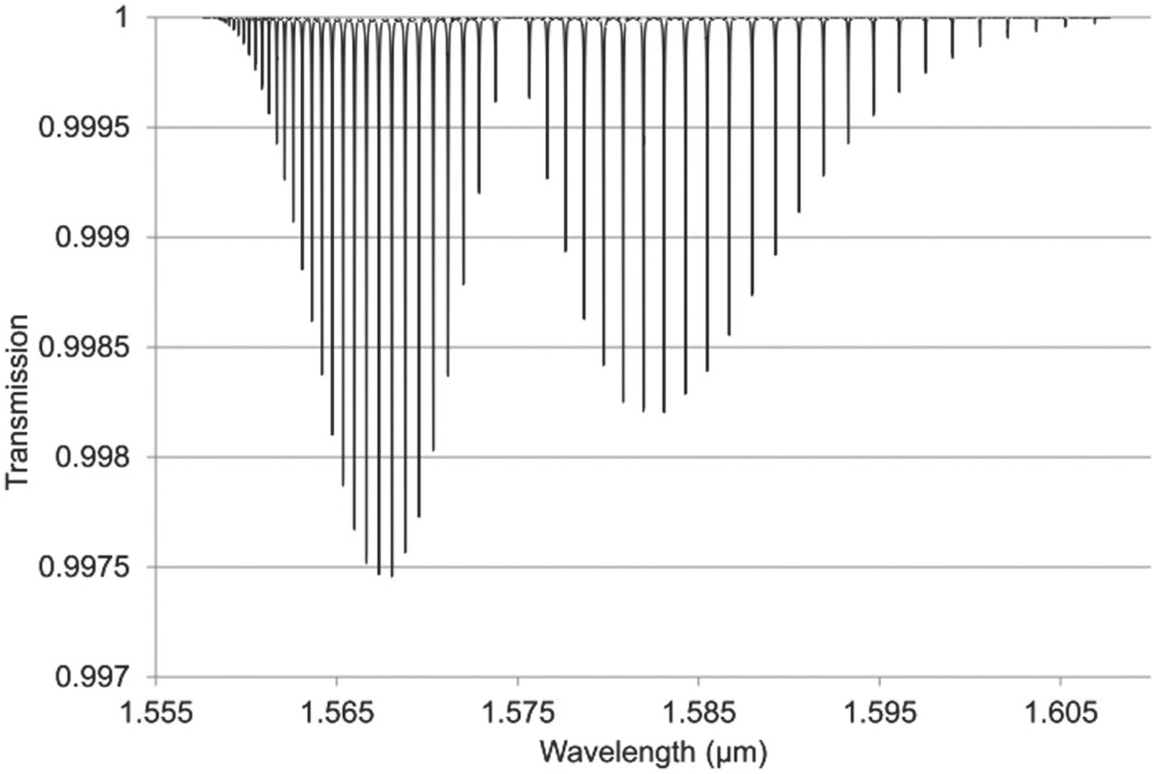
Figure 1.6 Near-IR absorption lines for CO plotted using HITRAN on the Web Reference Rothman[18].
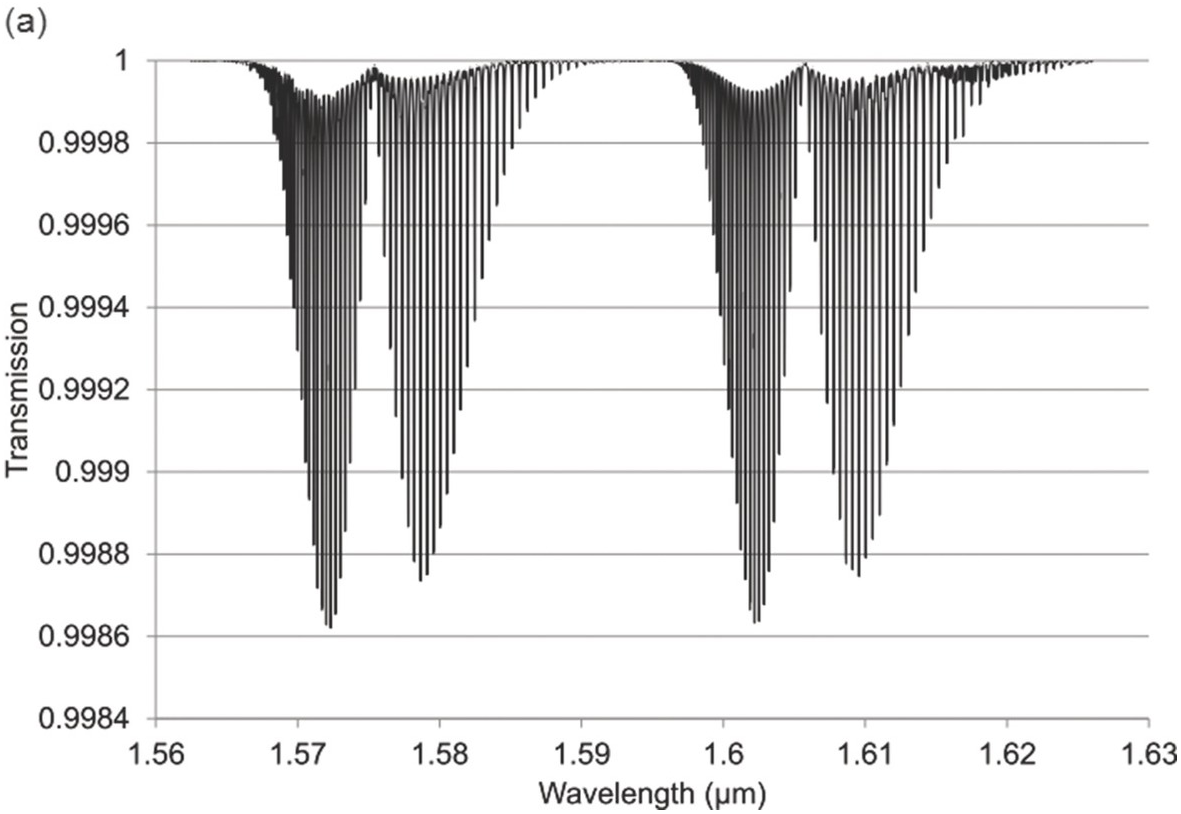
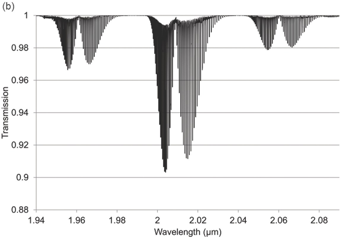
Figure 1.7 Near-IR absorption lines for CO2: (a) 1.6 μm region (b) 2 μm region plotted using HITRAN on the Web Reference Rothman[18].
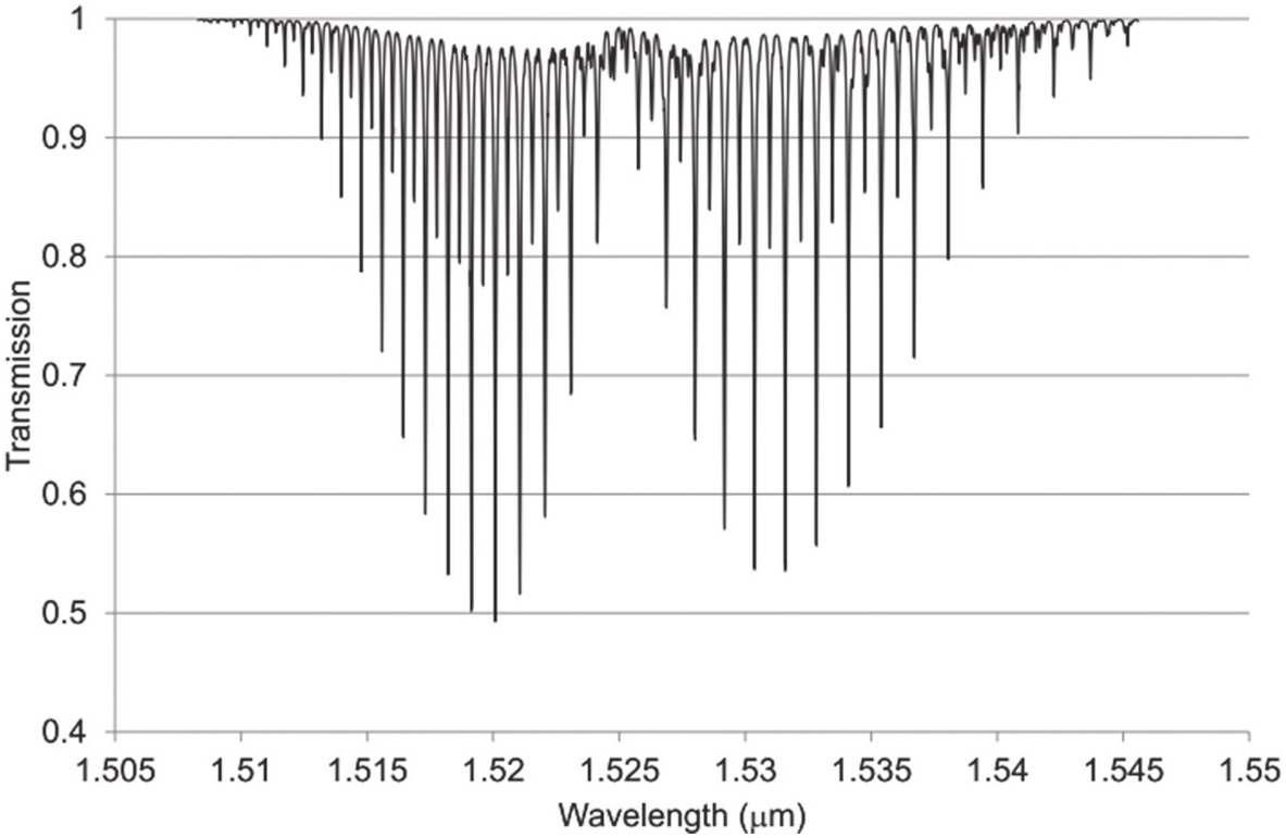
Figure 1.8 Near-IR absorption lines for C2H2 plotted using HITRAN on the Web Reference Rothman[18].
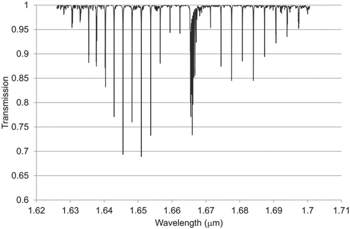
Figure 1.9 Near-IR absorption lines for CH4 showing the P, Q and R branches plotted using HITRAN on the Web Reference Rothman[18].
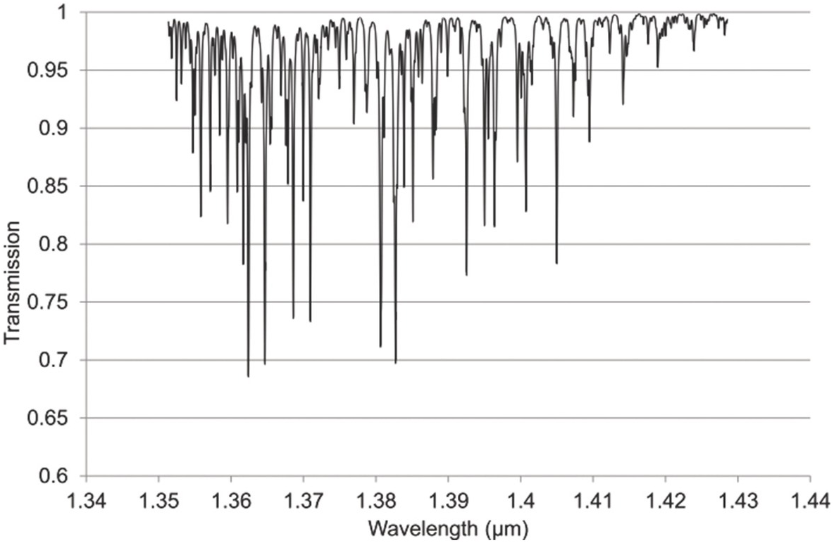
Figure 1.10 Near-IR absorption lines for H2O in the 1.4μm region plotted using HITRAN on the Web Reference Rothman[18].
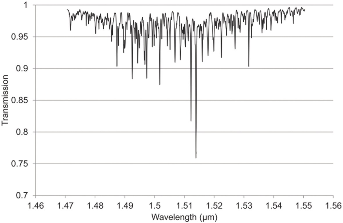
Figure 1.11 Near-IR absorption lines for NH3 plotted using HITRAN on the Web Reference Rothman[18].
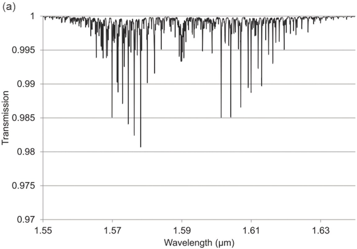
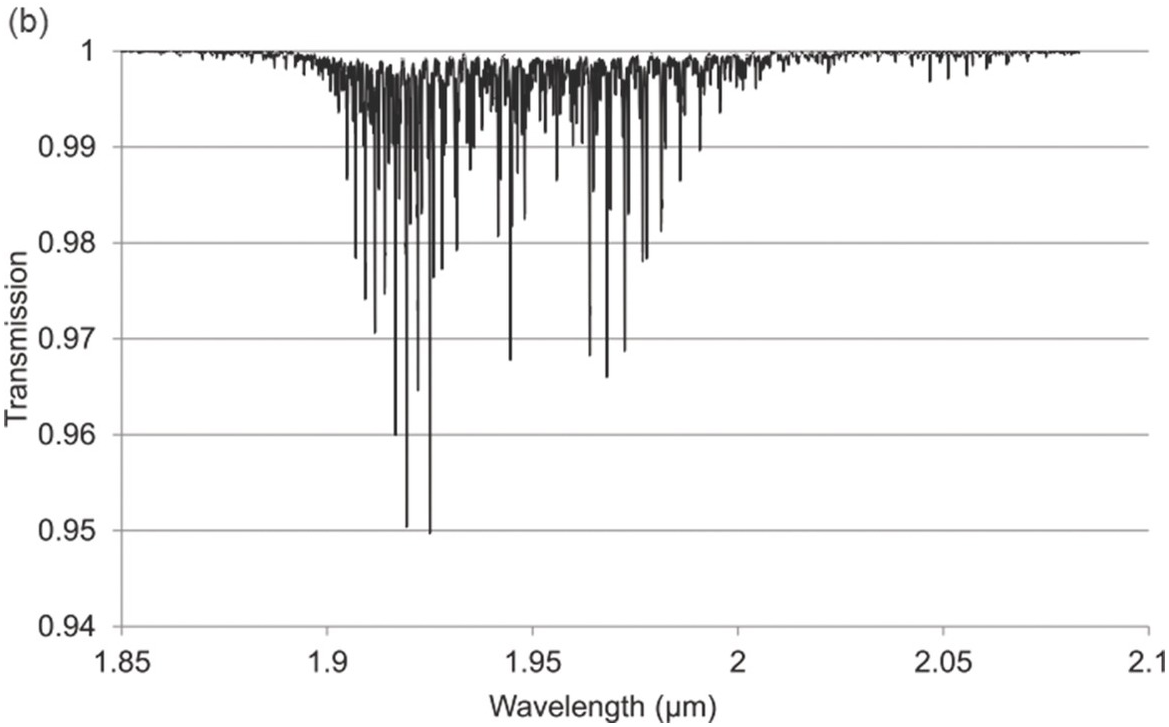
Figure 1.12 Near-IR absorption lines for H2S: (a) 1.6 μm region, (b) 1.9 μm region plotted using HITRAN on the Web Reference Rothman[18].
The absorption coefficient defined by (1.8) at line centre (in units of cm–1) for a particular line may be easily obtained from these figures as approximately the line depth when it is small or more accurately as α0 = −ln (Tmin) where Tmin is the line centre transmittance. The optical attenuation at line centre (in dB cm–1) is 4.34α0. Table 1.2 provides a list of the line centre absorption coefficient and attenuation for some absorption lines calculated from the figures, which will be useful later in discussing the sensitivity of near-IR and fibre optic systems. Similar data for a range of other gases may be obtained from HITRAN, including gases such as O2 which have no rotational or vibrational spectra but have electronic bands (O2 has a spectral band centred around 762 nm).
Table 1.2 Approximate values of line centre absorption coefficient and attenuation for common pure gases at atmospheric pressure and a temperature of 296 K
| Gas molecule | Wavelength of absorption line (µm) | α0 (cm−1) | Optical attenuation at line centre (dB cm–1) |
|---|---|---|---|
| Carbon monoxide (CO) | 1.5680 | 0.0025 | 0.011 |
| Carbon dioxide (CO2) | 1.5723 2.0035 | 0.0014 0.1 | 0.006 0.434 |
| Acetylene (C2H2) | 1.5201 | 0.69 | 2.99 |
| Methane (CH4) | 1.6510 | 0.36 | 1.56 |
| Water vapour (H2O) | 1.3827 | 0.36 | 1.56 |
| Ammonia (NH3) | 1.5139 | 0.27 | 1.19 |
| Hydrogen sulfide (H2S) | 1.5781 1.9250 | 0.019 0.05 | 0.08 0.22 |
Note the characteristic shape of the intensity envelope of the P and R branches as clearly shown in Figures 1.6–1.8. This arises from the multiplication of two functions governing the population of the rotational levels, namely, the exponentially decreasing function describing the population of the J-th state following Boltzmann statistics and the linearly increasing degeneracy of the J-th state by the factor (2J + 1). An additional factor determining the population of rotational levels is the influence of nuclear spin Reference Banwell and McCash[10]. As a result, for linear molecules possessing a centre of symmetry such as CO2, alternate rotational levels in the P and R branches have zero intensity. For C2H2, the rotational lines alternate in strength due to the nuclear spin of hydrogen atoms (see Figure 1.8).
1.5 Relative Merits of Near-IR and Mid-IR Absorption Spectroscopy
As noted previously, absorption lines in the near-IR are typically two or three orders of magnitude weaker than the fundamental transitions. A question therefore arises as to why one would use near-IR lines when much higher sensitivity is possible in the mid-IR. Certainly if high sensitivity is the main consideration then the fundamental absorption lines in the mid-IR are clearly the best choice. However, for many practical situations, the sensitivities that can be achieved in the near-IR may be perfectly adequate and there are several other issues that should be considered when reviewing the relative merits of the near-IR compared with the mid-IR region of the spectrum:
(i) Laser sources: the vast fibre optic data communications market has led to the ready availability of low cost, compact laser sources in the near-IR region, particularly DFB lasers, which can be tailor-made for a wide range of near-IR wavelengths and are extremely flexible in terms of wavelength tuning and modulation through control of the diode current and temperature. There have, of course, been major advances in the availability and performance of mid-IR sources in the last decade, particularly with regard to the development of quantum cascade lasers, but mid-IR sources are currently more expensive and generally less mature than their near-IR counterparts.
(ii) Optical detectors: mid-IR detectors can perform as well as near-IR devices but may require cooling at longer IR wavelengths to maintain noise performance and again are generally more expensive.
(iii) Optical fibres: near-IR systems offer unprecedented levels of flexibility in the design of spectroscopic systems through use of standard optical fibres, fibre amplifiers and photonic components from the data communications market. Techniques borrowed from data communication systems such as spatial-, time- and wavelength-division multiplexing may be applied in principle for the design of multi-point and multi-gas sensors, with fibre amplifiers to boost signal powers as required. By contrast, while the performance of mid-IR fibres will no doubt improve with further research, they are currently more expensive and are limited to relatively short lengths from fibre losses and may, in some cases, suffer from durability issues.
We shall return to these issues in Chapter 8, where a review of sources, detectors and fibres for mid-IR gas absorption sensors is given.
1.6 1.6 Conclusion
This chapter has reviewed the fundamental parameters involved in the design of gas absorption sensors, particularly for deciding appropriate wavelengths of operation, for predicting the expected sensitivity and for the extraction of concentration, pressure and temperature under different conditions of operation. The focus here is on near-IR spectroscopy since it is always prudent to consider this spectral region first to ascertain whether the required sensitivity for an optical gas sensor could be met with low-cost near-IR photonics. Of course certain gases may not possess suitable near-IR lines or their intensity may be too weak, in which case there is no option but to use the mid-IR spectral region, as reviewed in the last chapter of this book. However, near-IR systems will no doubt always have an important role in gas spectroscopy due to the maturity, low cost and versatility of sources, detectors and photonic components in this region of the spectrum.


