1 INTRODUCTION
Smoothed particle hydrodynamics (SPH) is a Lagrangian hydrodynamics modelling technique developed independently by Lucy (Reference Lucy1977) and Gingold & Monaghan (Reference Gingold and Monaghan1977). In this grid-less technique, fluid elements are represented by individual particles that act according to hydrodynamic flow equations. SPH has been used to model a wide variety of astrophysical phenomena, including star formation (e.g., Monaghan & Lattanzio Reference Monaghan and Lattanzio1991; Bonnell & Bastien Reference Bonnell and Bastien1992; Whitworth Reference Whitworth1998), planet formation (e.g., Benz, Slattery, & Cameron Reference Benz, Slattery and Cameron1986; Mayer et al. Reference Mayer, Quinn, Wadsley and Stadel2002; Nelson, Benz, & Ruzmaikina Reference Nelson, Benz and Ruzmaikina2003), cosmology (e.g., Navarro, Frenk, & White Reference Navarro, Frenk and White1995a, Reference Navarro, Frenk and White1995b; Springel Reference Springel2005), stellar collisions (e.g., Benz & Hills Reference Benz and Hills1987; Rasio & Shapiro Reference Rasio and Shapiro1991; Davies, Benz, & Hills Reference Davies, Benz and Hills1991, Reference Davies, Benz and Hills1992), stellar mergers (e.g., Rasio & Shapiro Reference Rasio and Shapiro1992; Terman, Taam, & Hernquist Reference Terman, Taam and Hernquist1994; Davies et al. Reference Davies, Benz, Piran and Thielemann1994; Rosswog et al. Reference Rosswog, Liebendörfer, Thielemann, Davies, Benz and Piran1999; Lee, Kluzniak, & Nix Reference Lee, Kluzniak and Nix2001; Fryer & Heger Reference Fryer and Heger2005; Yoon, Podsiadlowski, & Rosswog Reference Yoon, Podsiadlowski and Rosswog2007; Motl et al. in preparation), gas dynamics in the Galactic centre (e.g., Rockefeller et al. Reference Rockefeller, Fryer, Melia and Warren2004, Reference Rockefeller, Fryer, Baganoff and Melia2005; Cuadra et al. Reference Cuadra, Nayakshin, Springel and Di Matteo2005), galaxy mergers (e.g., Hernquist & Mihos Reference Hernquist and Mihos1995; Mihos & Hernquist Reference Mihos and Hernquist1996; Thakar & Ryden Reference Thakar and Ryden1998; Cox et al. Reference Cox, Jonsson, Primack and Somerville2006; Khalatyan et al. Reference Khalatyan, Cattaneo, Schramm, Gottlöber, Steinmetz and Wisotzki2008), and supernovae (Fryer & Warren Reference Fryer and Warren2002; Hungerford, Fryer, & Warren Reference Hungerford, Fryer and Warren2003; Fryer, Hungerford, & Rockefeller Reference Fryer, Hungerford and Rockefeller2007).
Each SPH particle i has an associated size hi, its so-called smoothing length. Fluid properties such as temperature or density are smoothed according to a smoothing function W, which is referred to as the SPH kernel. The most commonly used kernel functions are cubic splines (Monaghan Reference Monaghan1992) that are non-zero only within two smoothing lengths of the particle.Footnote 1 Fluid properties at the location of a particle can then be calculated as a linear combination of the contributions from all neighbouring particles. Thus, it is essential for this technique to start out with initial conditions whose interpolation properties are as accurate as possible. In addition, the initial particle setup should be as close as possible to a configuration that would arise by itself in an SPH simulation.
Due to their well-known interpolation properties and ease of construction, the simplest setup schemes often arrange particles on a lattice. While there are many lattice configurations that could in principle be used to produce SPH initial conditions, we focus on three popular configurations—a simple cubic lattice, a cubic close-packed lattice, and a hexagonal close-packed lattice. The simplest such arrangement (and one of the most popular) is the cubic lattice configuration, which has been shown to be an unstable equilibrium configuration and has strong preferred directions along the x, y and z axes (Morris Reference Morris1996; Lombardi et al. Reference Lombardi, Sills, Rasio and Shapiro1999). Cubic close-packed and hexagonal close-packed lattices represent the two optimal and most efficient ways to pack spheres of equal sizes; they are stable against random perturbation and thus much preferred to a simple cubic lattice (Monaghan Reference Monaghan1992). We also include a comparison with a new configuration method based on a quaquaversal tiling of space that has recently been suggested for quasi-random initial conditions of cosmological N-body simulations (Hansen et al. Reference Hansen, Agertz, Joyce, Stadel, Moore and Potter2007).
To avoid geometrical effects, initial conditions are often perturbed and then relaxed into a stable configuration by applying a dampening force that is proportional to but directed against the particle velocities (e.g., Rosswog, Ramirez-Ruiz, & Hix Reference Rosswog, Ramirez-Ruiz and Hix2009). While this additional step before calculation is perfectly acceptable to produce low-noise initial conditions, it is computationally expensive and usually only viable for static initial conditions, as the net forces on the whole set of particles should vanish. In addition, there is no way to guarantee the exact configuration into which the particles will settle at the end.
Another major problem in setting up initial conditions for SPH is that many astrophysical simulations require very large dynamic ranges in density. In simulations of, e.g., the accretion flow in binary mass transfer, the convective region in core-collapse supernova engine models, or interactions between supernova remnants or stellar winds and the interstellar medium, the resolution requirements may not trace the mass, and a range of particle masses may be required to model the system. Large ranges of particle masses in SPH are undesirable and care must be taken when using a range of particle masses. However, setting up arbitrary initial conditions with a spatially varying resolution is an unsolved problem so far; the few previously proposed solutions have only been applicable in spherical symmetry (e.g., Fryer et al. Reference Fryer, Hungerford and Rockefeller2007; Rosswog et al. Reference Rosswog, Ramirez-Ruiz and Hix2009).
In this paper, we propose a solution to this problem inspired by weighted Voronoi tessellations (WVTs) and present a new method to set up SPH initial conditions with arbitrary, spatially varying resolution requirements. We describe requirements for an optimal setup technique in Section 2 and then review and compare existing popular particle setup methods in Section 3. To the best of our knowledge, this is the first comprehensive comparison of SPH setup techniques, despite the known importance of initial conditions for SPH simulations. We introduce our new setup in Section 4 and demonstrate its capabilities with examples in Section 5. In Section 6, we quantitatively compare this new setup method to existing techniques.
2 REQUIREMENTS FOR AN OPTIMAL PARTICLE CONFIGURATION METHOD
A method for generating initial SPH particle configurations should fulfil the following key requirements:
2.1 Isotropy
The resulting particle configuration should be locally and globally isotropic, i.e., it should not impose any particular preferred direction at any location in the simulation domain. The main reason for this requirement is the fact that shocks moving along a perfectly aligned string of SPH particles behave differently than in other directions (Herant Reference Herant1994). In addition, spatially correlated density perturbations can excite modes along these preferred directions.
2.2 High interpolation accuracy
The setup should be locally uniform to minimise noise in the density interpolation. Ideally, for a uniform resolution, the interpolation accuracy should be comparable to that of perfectly uniform lattice configurations. This interpolation accuracy should also worsen for non-uniform particle configurations. Any deviations should also be isotropic and have no preferred directions, in order not to excite non-physical modes in the simulation domain. This requirement is equivalent to enforcing a low particle noise.
2.3 Versatility
The ideal method should be able to reproduce any spatial configuration and should not impose any requirement for symmetry. In particular, this requires the method to work with interpolation of a tabulated data set and not require analytical solutions.
2.4 Ease of use
Ideally, the algorithm should either be publicly available as a stand-alone routine or be easy to implement on top of any existing SPH code.
3 POPULAR PARTICLE SETUP METHODS
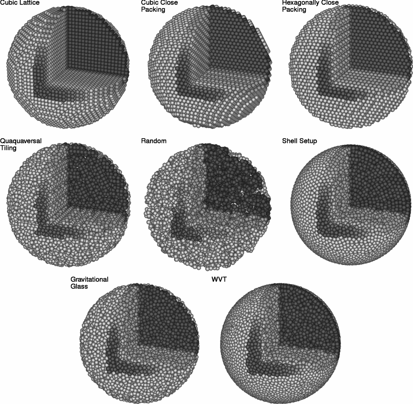
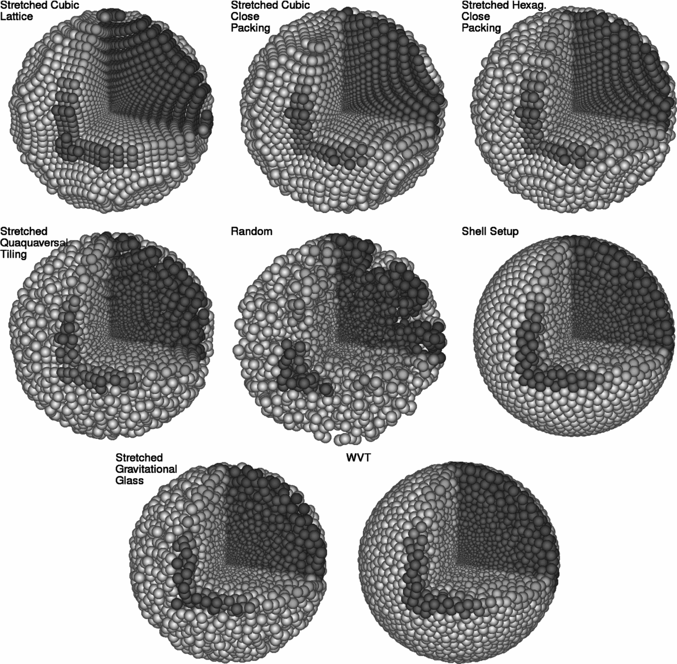
Since the invention of the SPH technique, many different methods have been employed to set up initial conditions in multiple dimensions. In this section, we summarise all particle setup methods known to us, or that have been described in the literature. Figure 1 shows a simple comparison of results of arranging approximately 22 000 particles with equal smoothing lengths in a sphere with each method. Figure 2 shows a similar comparison for spatially adaptive configurations, where the smoothing length varies across the domain (from smallest at the centre, to largest at the outer boundary). Section 3.1 describes the methods that are limited to producing configurations in which all particles have the same smoothing length; Section 3.2 describes the methods that can be used when smoothing lengths are not uniform. Readers who are already familiar with these methods or who are just interested in details of our method may examine the figures or skip this section entirely.
Popular configurations for setting up spatially uniform SPH initial conditions. From the top-left corner to the bottom right: cubic lattice, cubic close packing, hexagonal close packing, quaquaversal tiling, random configuration, concentrical shells, gravitational glass, and the new WVT approach. All examples contain approximately the same number of particles in the sphere (22 000). One quadrant of the sphere is cut out to allow a view into the inner configuration. Colours change along the z-axis simply to show depth.

Popular configurations for setting up spatially adaptive SPH initial conditions. From the top-left corner to the bottom right: stretched cubic lattice, stretched cubic close packing, stretched hexagonal close packing, stretched quaquaversal tiling, random configuration, concentrical shell setup, stretched gravitational glass, and the new WVT approach. All examples contain approximately the same number of particles in the sphere (22 000), and the particles’ sizes reflect the desired particle spacing. One quadrant of the sphere is cut out to allow a view into the inner configuration. Colours change along the z-axis simply to show depth.
3.1 Spatially uniform distributions
The following methods are capable of generating spatially uniform particle configurations.
3.1.1 Cubic lattice
Probably the simplest and fastest way to set up a uniform particle distribution is to arrange them on a cubic lattice. This method received early widespread use in both SPH (Monaghan Reference Monaghan1992) and N-body simulations (Efstathiou et al. Reference Efstathiou, Davis, White and Frenk1985). One of the obvious problems with this method is that it has very pronounced preferred directions along the x, y, and z axes and their diagonals, as can easily be seen in the upper-left example in Figure 1. In addition, the cubic lattice structure is not a stable equilibrium configuration when the particles are perturbed (Morris Reference Morris1996; Lombardi et al. Reference Lombardi, Sills, Rasio and Shapiro1999), as there are other more compact particle configurations that are energetically favourable, such as cubic or hexagonal close-packed arrangements.
3.1.2 Cubic close-packed lattice
A more compact lattice structure is produced when one inserts an additional particle into the centre of each of the six faces of the cubes in the cubic lattice. This results in the well-studied cubic close packing (CCP) configuration, also known as face-centred CCP (Figure 1, top centre panel). This configuration is one of the optimal ways to pack uniform spheres together, with a packing density of 74%. Similar to the cubic lattice, it has the problem of having preferred directions along the principal axes and diagonals of the lattice, and along multiple other planes in which particles are arranged in a hexagonal grid. However, these preferred direction are much less pronounced than for the cubic lattice configuration. The simplest way to construct this configuration is to start with a plane with spheres in a hexagonal configuration (plane A), and lay on top another such plane (B) so that the spheres fit into the gaps created by the layer of spheres from the lower plane, filling half the gaps. The third such plane (C) will then be oriented in a way to fill the other half of the gaps of plane A, while at the same time fitting into the gaps of plane B. This pattern is then continuously repeated to produce an ABCABC order.
3.1.3 Hexagonal close-packed lattice
A very similar lattice configuration is the second optimal packing scheme of uniform spheres, hexagonal close packing (HCP), as seen in the top-right panel of Figure 1. HCP is equally dense and optimal as CCP, with very similar properties. The only difference in its construction is that instead of the ABC pattern as in the CCP lattice, every second layer of hexagonal lattice planes is identical, resulting in an ABAB pattern. Due to their relatively simple implementation, close packing schemes have been utilised in many different applications of SPH (e.g., Davies et al. Reference Davies, Benz and Hills1991; Davies et al. Reference Davies, Benz and Hills1992).
3.1.4 Quaquaversal tiling
Another lattice-like particle configuration has been introduced by Hansen et al. (Reference Hansen, Agertz, Joyce, Stadel, Moore and Potter2007) based on a quaquaversal tiling of space (Conway & Radin Reference Conway and Radin1998). Quaquaversal tiling hierarchically tiles the 3D space into triangular prisms that are rotated about orthogonal axes 2/3 π and 1/2 π. Originally introduced as a way to set up cosmological initial conditions, recent work by Wang & White (Reference Wang and White2007) argues against this choice. As can be seen in the middle-left panel of Figure 1, this setup has many characteristics of a grid.
3.1.5 Gravitational glass
The best way to set up cosmological initial conditions however is the generation of a gravitational glass. This method simply reverses the sign of gravity and lets the particles settle into an equilibrium configuration while dampening their motion. In this paper, we use the implementation of a gravitational glass as provided in the publicly available gadget2 code (Springel et al. Reference Springel, Yoshida and White2001; Springel Reference Springel2005; Wang & White Reference Wang and White2007). This method is particularly effective when used with periodic boundary conditions. A cube with a fixed number of particles can then be replicated numerous times to achieve a larger total number of particles in the final configuration. While this is disadvantageous for cosmological N-body simulations, which require a certain degree of homogeneity on all scales, SPH only requires locally optimal configurations and is not affected by this. Thus, a single instance of a gravitational glass can be concatenated to effectively produce arbitrarily large particle configurations.
3.2 Spatially adaptive distributions
We now discuss the subset of setup methods that are capable of producing spatially adaptive particle distributions. To the best of our knowledge, all of these methods have so far been employed to create spherically symmetric configurations. Examples of each of these methods are shown in Figure 2.
3.2.1 Random configuration
The simplest option to produce a spatially adaptive particle configuration is to distribute particles randomly according to an underlying probability distribution. For example, Terman et al. (Reference Terman, Taam and Hernquist1994) have used this technique in combination with the relaxation method to create adaptive initial conditions. This relaxation is absolutely necessary, as this method results in very clumpy distributions with very low interpolation accuracy. We only mention this method as it represents the starting point for our new setup procedure described in Section 4.
3.2.2 Stretched lattice
To achieve a spatially adaptive resolution, Herant (Reference Herant1994) and later Rosswog et al. (Reference Rosswog, Ramirez-Ruiz and Hix2009) proposed to stretch a uniform lattice configuration in the radial direction. With this method, each point coordinate r of the uniform lattice is multiplied by a radially varying scaling factor q(r) to achieve the desired spherically symmetric distribution, such that r′ = q(r) r. This also implies through simple geometry that the given distance δ between two particle on the shell with radius r is now also scaled by q(r), effectively setting the resolution to δ′(r′) = q(r) δ.
Thus, the problem has now been reduced to figuring out how to choose q(r) to produce the desired resolution in the new stretched coordinates, i.e. δ′(r′) has to obey the differential equation r′δ(r) − rδ′(r′) = 0. While it is entirely possible to solve this problem analytically for simple δ′(r′) functions by substituting r′ and solving, it is more convenient to use a more generally applicable technique to find the root of the function f(r′) = r′δ(r) − rδ′(r′), with its derivative  $\text{d}f^{\prime }/\text{d}r^{\prime } = \delta (r) - r\,\text{d}\delta ^{\prime }(r^{\prime })/\text{d}r^{\prime }$. We chose the simple Newton–Raphson technique by iterating over $r^{\prime }_{n+1}=r^{\prime }_n+f(r^{\prime }_n)\,[\text{d}f/\text{d}r^{\prime }(r^{\prime }_n)]^{-1}$. Note that r is a constant parameter in this context, as it is given by the known position of the particle in the uniform lattice.
As this distorted lattice essentially incorporates and even aggravates all of the undesirable characteristics of a lattice configuration, it is essential not to use this stretched lattice configuration directly, but rather to relax the resulting configuration before using it in an actual SPH simulation (Rosswog et al. Reference Rosswog, Ramirez-Ruiz and Hix2009).
3.2.3 Stretched glass
Instead of radially stretching or compressing a uniform lattice configuration, it is also in principle possible to generate a gravitational glass of uniform resolution and stretch this glass accordingly, to avoid the strong preferred lattice symmetry axes. To the best of our knowledge, this method has never been employed in published simulations.
3.2.4 Concentric shells
In many supernova calculations using the Supernova SPH code (snsph) (e.g., Fryer & Warren Reference Fryer and Warren2002; Hungerford et al. Reference Hungerford, Fryer and Warren2003; Fryer, Rockefeller, & Warren Reference Fryer, Rockefeller and Warren2006; Fryer et al. Reference Fryer, Hungerford and Rockefeller2007; Fryer & Young Reference Fryer and Young2007), the initial conditions are set using shell templates. For a given particle count, such a shell template is created by first randomly placing the particles in a shell of unit radius. The particles are given a repulsive force and then the entire system is evolved until the variation in particle separation falls below some tolerance, essentially creating a two-dimensional gravitational glass wrapped around a sphere. The templates are then used to match a given spherical density profile and either a resolution or particle mass requirement. The spherical object is constructed from the inside outward, each concentric shell determining the new position of the next shell (one smoothing length above the previous shell). The shells are randomly rotated and placed on top of each other so that, even if the same template is used, the setup is random. A variant of this method had originally been proposed by Herant (Reference Herant1994) but to our knowledge has never been extensively described in the literature before.
The advantage of this technique is that the particles are placed randomly and hence have no preferred axis. Depending on the tolerance set for the template creation, the resolution used, and the density gradient, this technique can match a spherical density profile to arbitrary precision. For low-resolution core-collapse calculations, Fryer & Young (Reference Fryer and Young2007) achieved density perturbations below 3–5% (convection in the stellar models they were mapping argued for higher perturbations). For a high-resolution mapping of an exploding star, Fryer et al. (Reference Fryer, Hungerford and Rockefeller2007) limited this perturbation to below 1%. This technique is tuned to spherical objects, and does not work, without major revision, on aspherical objects.
4 A NEW APPROACH INSPIRED BY WEIGHTED VORONOI TESSELLATIONS
In this section, we describe a novel technique for generating spatially adaptive initial conditions for SPH simulations that does not impose any restrictions on the geometry of the desired configuration. This method was inspired by a two-dimensional adaptive binning technique using WVTs developed by Diehl & Statler (Reference Diehl and Statler2006), which in turn was based on previous work by Cappellari & Copin (Reference Cappellari and Copin2003).
4.1 Weighted Voronoi tessellations
Given a metric and a set of k points zi, i = 1, . . ., k (referred to as ‘generators’) in a given domain, a Voronoi tessellation of the domain is a tessellation in which the ith region contains all of the points closer to zi, according to the chosen metric, than to any other generator. A WVT applies a weight to the distance from each generator; a multiplicatively weighted Voronoi tesselation simply multiplies the distance from a given generator by its associated weight (see, e.g., Møller Reference Møller1994). The boundary surface b between adjacent regions in a multiplicatively weighted Voronoi tesselation is defined such that the scaled distance from each generator to the surface is equal, i.e.,
 $$\begin{equation}
|{\bf b}-{\bf z}_i|/\delta _i=|{\bf b}-{\bf z}_j|/\delta _j,
\end{equation}$$
$$\begin{equation}
|{\bf b}-{\bf z}_i|/\delta _i=|{\bf b}-{\bf z}_j|/\delta _j,
\end{equation}$$
if the metric is simply Euclidean distance, and where δi is a scale factor (i.e., the inverse of the weight) assigned to the ith generator.
A centroidal Voronoi tessellation (CVT) is a Voronoi tessellation where each generator coincides with the centroid of its region. Again, each generator can have an associated weight or scale factor, so that the sizes of the regions in the CVT vary across the domain.
One of the most well-known algorithms for constructing a CVT is the Lloyd algorithm (Lloyd Reference Lloyd1982), which alternates between constructing a Voronoi tessellation from a set of generators, and moving each generator to the centroid of its associated Voronoi region. The Lloyd algorithm is a special case of a general gradient descent approach to minimising the CVT energy function (Du & Emelianenko Reference Du and Emelianenko2006; Liu et al. Reference Liu, Wang, Lévy, Sun, Yan, Lu and Yang2009). It delivers monotonic, linear convergence to a CVT without the need for step size control (Du, Faber, & Gunzburger Reference Du, Faber and Gunzburger1999) but requires the ability to construct Voronoi tessellations, which is not a capability typically associated with implementations of SPH.
4.2 Technique
Our adaptive setup technique arranges particles by repeatedly applying net displacements based on proximity to neighbours and the desired final spatial resolution, which can vary across the problem domain. Identifying neighbouring particles and iteratively accumulating and applying pairwise displacements falls well within the normal capabilities of SPH codes.
Although we refer to it as ‘WVT’ because of the method that inspired it (Diehl & Statler Reference Diehl and Statler2006), our technique does not actually construct a WVT. The technique described below is similar to the distributed algorithm for constructing area-centred Voronoi configurations (Cortés, Martínez, & Bullo Reference Cortés, Martínez and Bullo2005; Martínez, Cortés, & Bullo Reference Martínez, Cortés and Bullo2007); each particle within a limited radius contributes to the calculation of a displacement in each iteration.
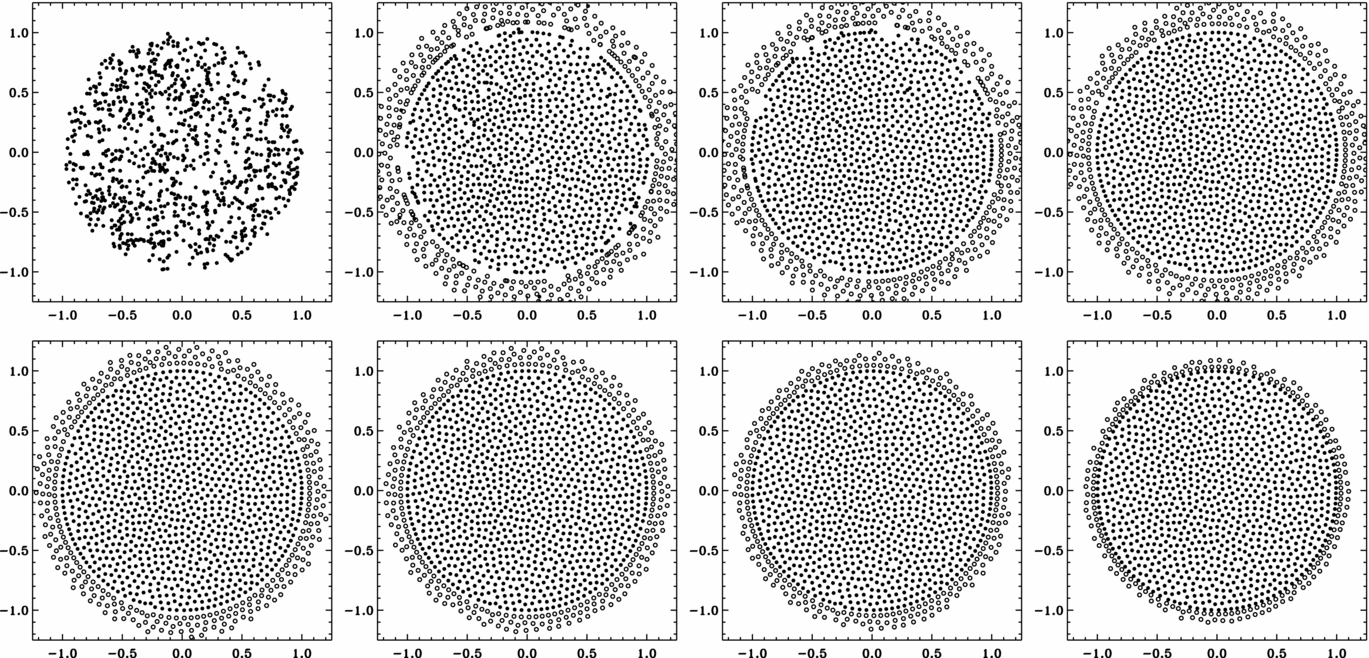
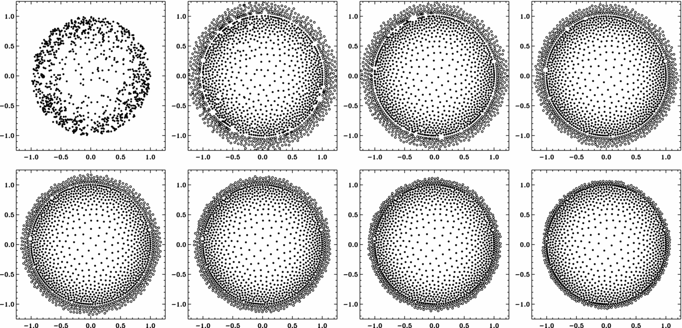
Given a desired average distance to neighbours δ(r) at each point r in the problem, the corresponding smoothing length h is determined by h(r) = N 1/nneigh (δ(r)/2) in n dimensions, where N neigh is the target number of neighbours. We construct an initial set of particles by sampling random positions according to the underlying particle probability distribution  $P({\bf r})\propto h({\bf r})^{-3}\text{d}V$ for a volume dV. We then evolve this configuration for multiple iteration steps by applying repulsive forces between the particles so they settle in the desired places. Figure 3 shows a two-dimensional example of the whole iteration process for a uniform distribution of particles, starting with the initial collection of particles in the upper left and ending with the final product in the lower right. Figure 4 shows an equivalent sequence for an azimuthally symmetric but non-uniform distribution. At the outer boundary, ghost particles exert a purely radial force on particles inside the domain, as if a smooth surface surrounded the domain, which leads to the formation of an unusually uniform ring of particles within 2h of the boundary. Such smoothness at the boundary might be an asset in some simulations—for example, if the simulation domain really is the inside of a sphere—but in other cases the outer particles simply behave like the outermost layer of a concentric shell configuration (Section 3.2).
Two-dimensional example for producing a uniform particle density in a circle with radius 1 with the new WVT setup for 1 000 particles. The frames show snapshots of the WVT iterations, starting with random positions sampled from a uniform distribution (top left), and then showing every 10th iteration, until the final product in the lower right panel (here, iteration 70). The hollow particles are ‘ghost particles’ that establish proper boundaries.
Same as Figure 3, but for a non-uniform particle distribution. The target particle density is four times higher at the edge of the circle than in the centre.
To reach a useful final configuration, these artificial forces should satisfy two main requirements:
1. The net ‘force’ on any particle should be zero (to a reasonable level of precision) in the desired equilibrium configuration, i.e., when the distance between two particles is identical (or very close) to the desired resolution.
2. The ‘forces’ should be such that the net displacement from the last position is on the order of a fraction of the desired resolution. This will ensure equally fast convergence for high and low-resolution regions of the problem.
Thus, Equation (1) dictates the value of the repulsive ‘displacement’ from bin j on bin i, which we express for simplicity directly as a net displacement
 $$\begin{equation}
\Delta {\bf x}_{i}=\sum \left[\mu \, h_{i}\,f(h_{ij},r_{ij})\,\hat{\bf r}_{ij}\right] = \mu \, h_{i} \sum \left[\,f(h_{ij},r_{ij})\,\hat{\bf r}_{ij}\right],
\end{equation}$$
$$\begin{equation}
\Delta {\bf x}_{i}=\sum \left[\mu \, h_{i}\,f(h_{ij},r_{ij})\,\hat{\bf r}_{ij}\right] = \mu \, h_{i} \sum \left[\,f(h_{ij},r_{ij})\,\hat{\bf r}_{ij}\right],
\end{equation}$$
with hij = (hi + hj)/2. The function f(hij, rij) should be compact within 2h, and empirical tests show fastest convergence of the method for a r −2 dependence. In practice, we add an ε term in the denominator to avoid numerical problems for close particles, and subtract a constant value to make sure the function value vanishes at the boundary at 2h and is set to 0 if the separation is larger than that. Thus, we can express the function as f(hij, rij) = [hij/(rij + ε)]2 + const. The value of μ in Equation (2) regulates what fraction of hij the particles are allowed to move during each iteration step. This free parameter should be chosen to ensure fast convergence. In practice, we shrink μ monotonically with the number of iterations, so particles can move relatively freely at the beginning and at the end ‘freeze’ into their final position. Note that the particle spacing δ(r) can be an almost arbitrary function of space, as long as its value does not change significantly across one particle spacing to ensure convergence of the method, i.e., Δδ(r)/δ(r) ≪ 1.
We chose the r −2 dependence as it reproduces locally many desirable properties of a gravitational glass. A functional form based on the SPH kernel would be another natural choice for this problem, though we did not thoroughly test this possibility.
4.3 Practical implementation
Here, we provide some practical advice on implementing the WVT setup on top of an existing SPH code.
4.3.1 Normalising h(r)
In our description of the WVT method above, we have assumed that we know a priori the desired particle spacing δ(r) as a function of position. However, it can be difficult to guess what specific spatial resolution, at each point in a complex problem, will produce a configuration with an acceptable total particle count. Thus, our implementation interprets the input particle spacing as a relative rather than an absolute value, and scales it according to a desired number of particles N SPH and neighbours N neigh. At each iteration step, h(r) is evaluated for all particle positions and we then compute the sum of all individual SPH particle volumes: V SPH = ∑i[(4π/3)(2 hi)3]. Since we do know the actual volume V of our computational domain and that we desire N neigh neighbours within 2h for each particle, we scale all h(r) values so that V = V SPH/N neigh.
4.3.2 Treating boundaries
Most modern SPH codes have some kind of boundary treatment already implemented. Fixed boundaries are usually implemented by means of ghost particles (e.g., Herant Reference Herant1994) that exert antisymmetric forces on the particles to keep them across a given boundary. WVT works well with this type of boundary treatment, and we suggest mirroring SPH particle layers within two smoothing lengths at the boundary interface and adding them to the set of normal particles during the pseudo force calculation step. Periodic boundaries may also be used, and the region of interest can simply be ‘cut out’ afterwards. We find this method to work well for arbitrary geometries.
4.3.3 Updating particle positions
The most convenient way to implement WVT is to use the entire structure of your existing SPH code with as few changes as possible. We suggest modifying the existing SPH loop to calculate the sum in Equation (2) and then multiply this pseudo ‘velocity’ by the ‘individual time steps’ μhi to update particle positions. If the distribution does not appear to converge, we suggest decreasing the value of μ with each iteration.
4.3.4 Finishing the iterative process
Judging when an initial setup is sufficiently good is application dependent and at least somewhat subjective. In our experience, slowly reducing the value of μ (the maximum fractional distance a particle can be moved in one time step; see Equation (2)) works well. For the cases we have studied, which include setups using from 100 000 to 50 million particles (Raskin et al. Reference Raskin, Timmes, Scannapieco, Diehl and Fryer2009, Reference Raskin, Timmes, Scannapieco, Diehl and Fryer2010; Fryer et al. Reference Fryer2010; Passy et al. Reference Passy2012; Ellinger et al. Reference Ellinger, Young, Fryer and Rockefeller2012), convergence occurs in about 100 iterations, usually even after only 40 iterations. However, this number may strongly depend on the details of the algorithm, and the desired interpolation accuracy, an issue that we discuss in more detail in Section 6.
5 EXAMPLE APPLICATIONS
Different applications may impose very different requirements on the resolution of a particular object. When particle mass density and desired number density vary together, WVT can generate initial conditions with particles of uniform mass; when the mass density and desired number density vary in different ways, WVT can produce configurations where both particle mass and size vary across the domain. We now consider different examples, mostly from stellar interactions, that impose very different numerical requirements.
5.1 Uniform particle density
In the first application, we consider representing a star with a uniform particle density, which would be appropriate for simple head-on collisions between two stars. In this situation, it is very likely that both centre and outer layers will be heavily involved in the process, as all parts should be equally affected during the merger, and would require equal resolution to resolve hydrodynamic effects throughout the star.
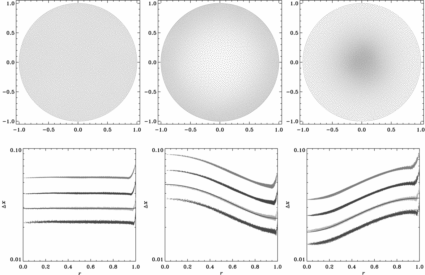
Such a 2D particle setup is shown in the top-left panel of Figure 5. The lower panel shows how well the desired resolution is achieved by measuring the average distance between particles for the closest 8 (red), 16 (green), 32 (blue) and 64 (orange) neighbours. The black solid line shows the expected theoretical values for 16 neighbours. The deviations at the boundary are due to the lack of neighbours across the boundary, and can of course be fixed by increasing h accordingly in that region.
Top panels: particle configurations in two-dimensional examples. We consider three different configurations: uniform particle density (left), more resolution in outer layers (centre), more resolution at centre (right). The bottom panels shows the actual particle separations as a function of radius. The points measure the average distance to the closest 8 (red), 16 (green), 32 (blue) and 64 (orange) neighbours. The solid black line shows the input resolution scaled for the closest 16 neighbours, indeed closely following the green data points.
5.2 More resolution in the centre
However, if the user is interested in any type of mixing within the stars or during a merger, it is imperative to use equal-mass particles. Work by Lombardi et al. (Reference Lombardi, Sills, Rasio and Shapiro1999) suggests that artificial forces between non-equal-mass particles lead to numerical diffusion and artificial mixing. With the WVT setup, we can enforce equal mass particles by adjusting the particle separation according to the underlying density ρ(r), such that δ(r)∝ρ(r)−1/3. This results in a setup with more resolution in the centre, as shown in the right panel of Figure 5.
5.3 More resolution in the outer layers
If one is interested in studying the more gentle Roche Lobe overflow phase in a binary, one needs as much numerical resolution as possible in the outer layers of the donor star, in order to sufficiently resolve the overflow and accretion stream. The middle panel of Figure 5 shows a polytrope where we have put more resolution in the outermost layer than in the centre.
5.4 Asymmetric initial conditions: Double degenerate binary
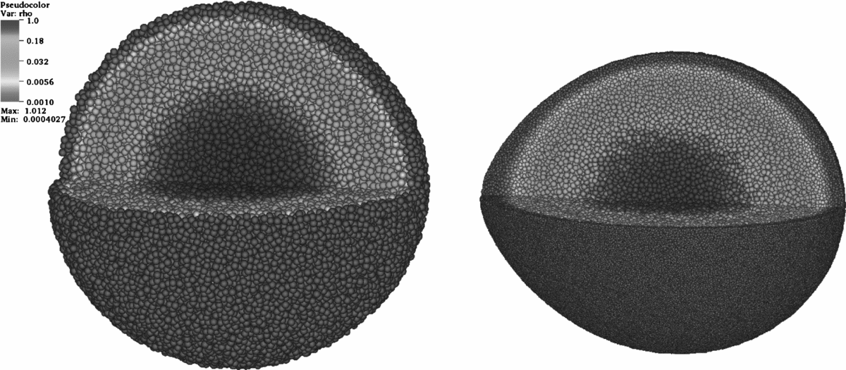
Figure 6 shows an example of an asymmetric, three-dimensional setup with WVT. The picture depicts a double degenerate binary system with the donor (right) on the verge of overflowing its Roche lobe. Note how the size of the SPH particles (varying sizes and colours of spheres) is much smaller in the outer layers of the donor, which helps significantly in resolving the mass transfer stream in the simulation (Motl et al. in preparation). The evolution of the system is extremely sensitive to the initial mass transfer (as it governs the evolution of the orbit). Resolving this mass transfer is critical to achieving good agreement between SPH and rotating grid simulations.
This three-dimensional example shows an asymmetric WVT setup for a double degenerate merger simulation. In this example, the accretor (left) is modelled with a constant particle density, whereas the donor (right) has significant more resolution in the outer layers than in the centre, making SPH simulation of Roche lobe overflow feasible.
5.5 Asymmetric initial conditions: Elliptical galaxies
Simulations of normal elliptical galaxies commonly use a gas component embedded within a dark matter halo in order to model evolution properly. Creating an initial configuration for a simulation of feedback effects in such a galaxy, it is reasonable to say the gas has settled hydrostatically into the dark matter potential and is quiescent. We assume that the gravitational effects of the gas are small compared to those of the dark matter. Then, we should expect the gas density ρgas to follow the dark matter potential ΦDM, assuming a polytropic equation of state:
 $$\begin{equation}
\rho _{\rm {gas}}(x,y,z) = \left[ \frac{-1}{K (n+1)} \Phi _{\rm {DM}}(x,y,z) + C \right] ^{n}
\end{equation}$$
$$\begin{equation}
\rho _{\rm {gas}}(x,y,z) = \left[ \frac{-1}{K (n+1)} \Phi _{\rm {DM}}(x,y,z) + C \right] ^{n}
\end{equation}$$
where K is a constant, n is the polytropic index, and C is a constant of integration that determines the sharpness of the edge of the density distribution. Note that ρgas and ΦDM need not be spherical in shape; the dark matter potential maps into the gas density regardless of its degree of eccentricity.
In fact, we may take direct advantage of the non-requirement for spherical shape; the WVT code contains an option to use a cloud of dark matter particles as three-dimensional interpolation points in order to determine the value of the dark matter potential at a given position. Then, Equation (3) defines the mass density for a gas particle placed at that point.
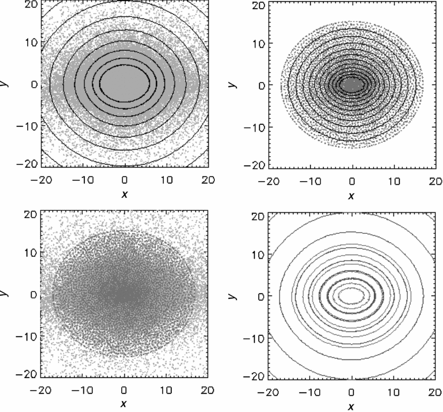
If Equation (3) is applied correctly, the resulting surfaces of constant gas mass density must coincide with the surfaces of constant dark matter potential. Thus, as a diagnostic test, we first construct a self-consistent Hernquist sphere of N-body particles with a distribution function of Ossipkov–Merritt form (Osipkov Reference Osipkov1979; Merritt Reference Merritt1985a, Reference Merritt1985b; Kazantzidis, Magorrian, & Moore Reference Kazantzidis, Magorrian and Moore2004) and anisotropy radius r a = 1 × 10¹⁰, and then use the method of Holley-Bockelmann et al. (Reference Holley-Bockelmann, Mihos, Sigurdsson and Hernquist2001) and Widrow (Reference Widrow2008) to deform the sphere adiabatically into a triaxial system. The resulting configuration of N-body particles has approximate axis ratio 17:15:14, and forms the set of interpolation points from which to create a cloud of gas particles via WVT. The example gas cloud analysed in Figure 7 has a polytropic index of n = 3/8, and shows gas isodensities coincident with the dark matter isopotentials.
WVT results for a gas cloud with polytropic index of n = 3/8, embedded within a triaxial (axis ratio 17:15:14) dark matter potential, a slice through the simulation at z = 0. Top left: Dark matter particles in cyan, with surfaces of constant potential overplotted. Top right: SPH gas particles in red, with surfaces of constant mass density overplotted. Bottom left: SPH gas particles in red and dark matter particles in cyan. Bottom right: The surfaces of constant dark matter potential (blue) coincide with the surfaces of constant gas mass density (red).
5.6 Asymmetric initial conditions: WVT logo
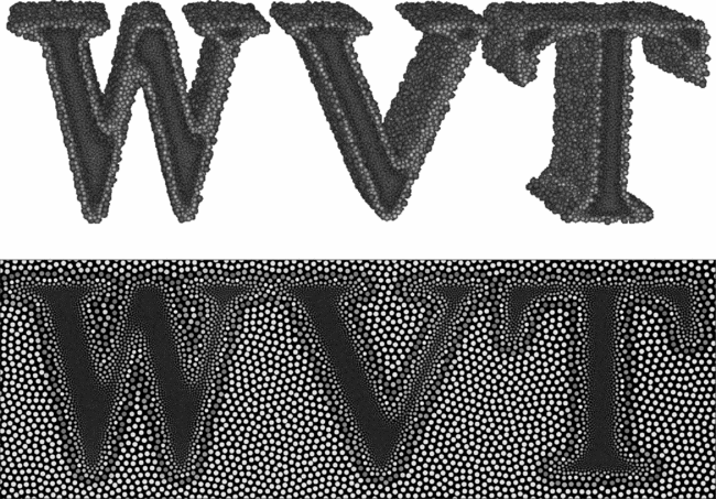
Figure 8 shows another example of an arbitrarily complex setup. The top panel shows the letters ‘WVT’ used in three dimensions, the lower panel gives the same example in two dimensions. Note that we omitted the largest SPH particles (white particles in the 2D version) in the 3D version for clarity. WVT has no difficulties in matching the desired resolution even in these complex test cases.
Examples for an arbitrary spatial configuration. The top panel shows a 3D configuration, the lower panel shows a two-dimensional configuration. Particles with large smoothing lengths (shown in white in bottom panel) are omitted in the three-dimensional view for clarity. This particular configuration shows a dynamic range of ~ 10. Smoothing lengths are indicated by colour and proportional to their symbols’ sizes.
5.7 Mixing in supernovae
As the shock moves out through a star in a supernova explosion, Richtmyer–Meshkov and Rayleigh–Taylor instabilities drive turbulence behind the shock. This turbulence mixes elements, dredging up radioactive 56Ni and injecting hydrogen into slower moving layers. This mixing is observed in supernova light-curves and in the knots in supernova remnants. But modelling this turbulence is not trivial; the shock radius expands by several orders of magnitude, and both cartesian grid Eulerian and SPH codes introduce numerical turbulence (based on noise in the initial setup) that can artificially produce spurious turbulence.
The Sedov blast wave is an ideal test for any code modelling these explosions; an analytic solution exists and can be compared to simulation results. This test also exposes consequences of choices in initial conditions beyond just total particle or mesh cell count. Approximating a point explosion in a large volume benefits from higher spatial resolution near the origin, and the shock is often unstable to hydrodynamic instabilities (e.g., Richtmyer–Meshkov and Rayleigh–Taylor behind the shock), so any initial density perturbation introduced by the setup (or grid effects in an Eulerian code) can artificially seed turbulence.
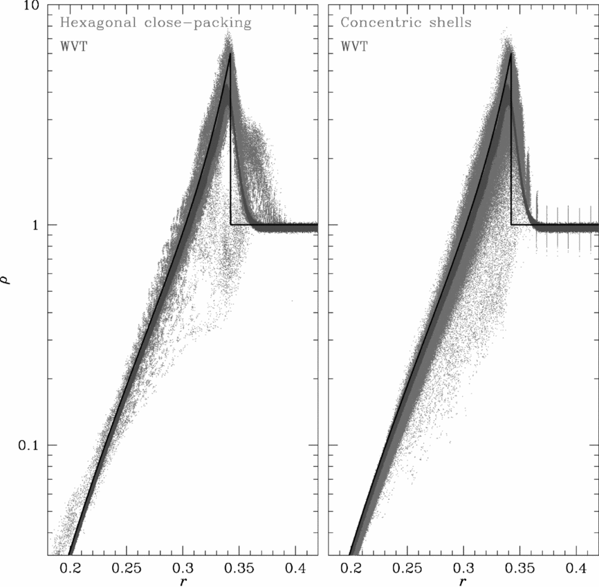
With a given total particle budget, different schemes for generating initial conditions have different degrees of success in meeting the resolution, homogeneity, and isotropy requirements of Sedov simulations. Figure 9 shows the particle distribution, in terms of mass density versus radius, for three different simulations of a Sedov blast wave—one using a hexagonal close-packed lattice, one using a concentric shell configuration, and one using WVT—at a time t = 0.06317 after the launch of the shock. The number of particles is nearly identical for each simulation (1.52 million for the shell setup, 1.50 million for the hexagonal close-packed and WVT configurations). The black line in the figure indicates the analytic solution at this time. All three simulations used the same gamma-law equation of state, with γ = 7/5.
Density versus radius of a Sedov blast wave problem comparing the results from a WVT setup with a hexagonal close-packed lattice (left) and a concentric shell configuration (right), each using 1.5 million particles. The black line indicates the analytic solution. In the hexagonal close-packed lattice, different shock velocities at different angles through the lattice lead to variation in the shock position around the sphere—and to lower-density regions behind the fastest parts of the shock, which show up in the plot as extra scatter in density, especially for radii between ~ 0.32 and ~ 0.36, at this time in the simulation. The initial density perturbations in the concentric shell setup—visible as scatter in density at constant radius outside the shock—grow in the shock to produce a broad range of particle densities. The low resolution at the energy source leads to velocity perturbations that then create density perturbations.
In the same way that initiating a Sedov blast wave calculation by injecting energy into a single mesh cell could imprint the mesh geometry onto the resulting shock, initiating a calculation by injecting energy into a single SPH particle at the origin could produce an aspherical explosion imprinted with artefacts of the arrangement of neighbouring particles. In each of the three simulations, energy E = 1 was injected into a small spherical volume at the centre of the simulation at t = 0. The radius of that volume varied among the simulations, according to the competing constraints that it be as small as possible, to initiate a point-like explosion, but large enough to extend out to several times the smoothing length of the innermost particles, to eliminate relics of the specific particle arrangement around the origin.
A uniform lattice is, by definition, poorly suited for problems with spatially varying resolution requirements. The goal was to simulate a Sedov blast wave in a sphere of radius r max = 1, but the hexagonal close-packed lattice compromised at both small and large radii; with a uniform spacing of 0.01 between closest neighbours, it extended out only to r max = 0.63. At the same time, the uniform lattice had limited ability to simulate a point-like explosion; energy was smoothed over particles at radii r < 0.024, which included 81 particles.
Though both the concentric shell setup and the WVT setup covered a larger range of radii, using the concentric shell setup for Sedov simulations requires extra attention to the compromise between radial and angular resolution. Increasing the particle count for a given shell tends to reduce variation in density around the sphere at that radius, but spending the particle budget on angular resolution requires reducing the overall number of shells, and having too few shells per neighbourhood can lead to radial fluctuations in density and velocity.
Both the concentric shell setup and the WVT setup extended from r max = 1 (where the largest particles had smoothing lengths h max = 2.62 × 10⁻² in the concentric shell setup and h max = 3.29 × 10⁻² in the WVT setup) to much smaller scales; near the origin, the smallest particles had smoothing lengths h min = 7.81 × 10⁻³ in the concentric shell setup and h min = 2.69 × 10⁻⁴ in the WVT setup. In the concentric shell setup, energy was smoothed over particles at radii r < 3.9 × 10⁻³, or the innermost 10 shells (containing a total of 4 840 particles); in the WVT setup, energy was smoothed over particles at radii r < 5.0 × 10⁻³, which included 38 148 particles. Particles had an average of 54 neighbours in the hexagonal close-packed lattice, 76 neighbours in the concentric shell setup, and 50 neighbours in the WVT setup.
As the shock expands outwards, the variation of resolution with radius among the three sets of initial conditions becomes apparent; at t = 0.06317, there are 481 562 shocked particles in the simulation using the shell setup, only 190 472 in the hexagonal close-packed simulation, and 977 512 in the WVT simulation.
In the hexagonal closed-packed lattice, the shock propagates faster along lattice planes than in other directions. This leads to a radial spread in the apparent shock location, averaged over the sphere, and areas of lower density behind those advanced parts of the shock that show up especially between radii 0.32 < r < 0.36, at this time in the simulation. A WVT setup with the same uniform particle spacing avoids this angle-dependent behaviour, which eliminates the appearance of faster-than-expected features ahead of the shock, and most of the variation in density at a given radius. When used to generate initial conditions with spatially varying resolution, WVT produces much less scatter with the same total particle count, limiting the numerically seeded turbulence in this problem.
The nature of the concentric shell setup introduces a density perturbation within each shell, visible as scatter in density at discrete radii outside the shock in the right panel of Figure 9. This perturbation grows when the shock passes through it, driving strong density perturbations and convection. In simulations of supernova explosions (e.g., Fryer et al. Reference Fryer, Hungerford and Rockefeller2007) and other more complex environments, ensuring that these perturbations are small compared to perturbations expected in the natural system can require several rounds of setup, simulation, and adjustment. Even with the same innermost radius and particle size, WVT produces a smoother representation of the initial conditions in both radius and angle; in the simulations presented here, WVT was used to produce a configuration with a smooth representation at even smaller radii, supporting a smaller energy injection region containing more particles.
The WVT setup underestimates the density both behind and ahead of the shock—by 6.6% for particles between r = 0.2 and 0.25, 9.3% between r = 0.25 and 0.3, 15.4% between r = 0.3 and the shock, and 2.9% in the unshocked region between r = 0.37 and 0.41. Both the hexagonal closed-packed and shell configurations provide better estimates of the density ahead of the shock—overestimating by 0.95% and 1.9%, respectively. Behind the shock, the average density for the shell configuration is consistently lower than the WVT result—15.5% below the analytic value for particles between r = 0.2 and 0.25, 14.4% low between r = 0.25 and 0.3, and 13.6% low between r = 0.3 and the shock. The average density in the hexagonal close-packed simulation is just slightly above the analytic line—by 0.6%—for particles between r = 0.2 and 0.25, and below the target value by 6.7% between r = 0.25 and 0.3, and by 14.7% between r = 0.3 and the shock, but averaging over all particles at a given radius in this calculation hides significant variation between different angles around the sphere. For both the shell setup and WVT, the iterative process of assigning masses to particles given their initial position and spacing could be improved to better match the desired initial density profile.
6 COMPARISON TESTS
6.1 Interpolation accuracy: Uniform density
An important performance test for any SPH setup method is to find out how well it reproduces a given density field. This test will reveal the level of perturbations that are introduced by the setup, which could seed convection, excite sound waves, or trigger instabilities. The simplest such test is to see how well each method can mimic a uniform density field with a uniform particle distribution. Thus, each particle should have the same mass, which we will assume to be 1, and the same smoothing length/resolution. At the same time, this test will then provide a means to test the accuracy of the particle density distribution itself.
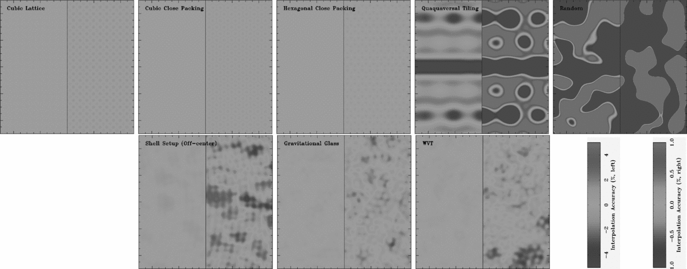
Figure 10 shows the accuracy of all uniform density methods described in Section 3, along with the new WVT method. Each panel shows a projection of a unit cube containing 8 000 particles onto the x–y plane according to the standard spline SPH kernel targeted at containing approximately 128 neighbours. We divided each figure into two parts, with the colours in the left half showing up to 5% deviations (negative: blue, positive: red, accurate: green), whereas the right half reveals lower level (up to 1%) deviations.
Comparison of the interpolation accuracy for 128 neighbours in the cubic lattice, cubic close packing, hexagonal close packing, quaquaversal tiling, random configuration, shell setup, gravitational glass, and the new WVT approach (top left to bottom right). Colours indicate deviations from the target density, with blue colours showing negative and red colours denoting positive deviations. Each panel is divided into two halves with different dynamic ranges: ± 5% on the left and ± 1% on the right side. Note that the shell setup is shown at an off-centre location, to avoid the discussed special treatment of the centre in this comparison. Quaquaversal tiling and the random setup perform noticeably worse than any other method, while the uniform grid setups perform best as expected. The non-gridded setup methods perform equally well, with very high interpolation accuracies that never exceed 1%.
The first three panels show the lattice configurations (cubic lattice, CCP, and HCP) which obviously have excellent interpolation properties. This is not surprising, as they are designed to be as uniform as possible, and each particle has an identical number of neighbours. Only in the right half of each panel does low-level noise becomes visible, revealing the underlying lattice structures. Note that the CCP panel shows hexagonal structures, as the x–y plane cuts through a hexagonal layer. Other orientations of the plane would reveal different patterns, but give the same qualitative impression.
The fourth panel in the top row shows the quaquaversal tiling configuration, which demonstrates very strong clustering of particles and corresponding deviations from the ideal values. Even with 128 neighbours, density fluctuations on the order of 5% are found throughout the simulation volume. In addition, these deviations are strongly spatially correlated, which makes numerical artefacts likely. This reason alone is grounds enough not to use quaquaversal tiling for SPH setups. This effect has also recently been pointed out by Wang & White (Reference Wang and White2007), who found that using quaquaversal tiling to initialise cosmological situations leads to an excessive amount of small halos and clumping. In fact, the only setup method that produces stronger density fluctuations is placement of particles randomly throughout the simulation domain (top-right panel).
The first panel in the lower row shows the interpolation accuracy of the shell setup, at an off-centre location. This setup has most often been used for simulations with an inner boundary inside the innermost shell of particles, which excludes that central volume from the simulation domain. (In a simulation that extends all the way to r = 0, interpolation accuracy inside the innermost shell will be poor without special treatment. Options include placing a small lattice configuration, a gravitational glass configuration, or a single particle inside the innermost shell; the former two can still produce artefacts near the innermost shell, while the latter works best if the innermost shell radius is about the same as the typical inter-particle separation within the shell.) Similar to the lattice configurations, individual shells are visible as low-level noise in the right half of the panel. The level of noise in the density interpolation for 128 neighbours is on the order of 1%, consistent with findings by Fryer et al. (Reference Fryer, Hungerford and Rockefeller2007). However, note that the setup is only optimised within one shell, which leads to the noise deviations having a preferred radial direction perpendicular to the shell structures.
Within one shell, the setup has similar properties to a uniform gravitational glass, shown in the second panel of the bottom row. The level of noise for this method is very low, generally on the order of 0.5% at most. Also note that the noise is isotropic with no preferred direction, as is true for the underlying particle distribution. These desirable properties make the gravitational glass setup a suitable choice for uniform density distributions.
The last panel in the bottom row shows the interpolation properties of our new WVT setup method. Note the similarity to the gravitational glass, with an equally low amount of noise and an isotropic distribution of the noise without preferred directions. In our WVT implementation, each repulsive force is roughly proportional to r −2, and the ratio of scale lengths is 1 for a uniform distribution, which makes the WVT setup locally very similar to a gravitational glass.
In summary, the three uniform lattices (cubic lattice, CCP, HCP) have excellent interpolation characteristics for a uniform density and should be used in situations where lattice effects are expected to be unimportant, but a very low level of initial numerical noise is needed. The quaquaversal and random initial condition are unacceptable for any application due to their low interpolation accuracy. In spherical symmetry, the shell setup provides an adequate configuration, but without a special treatment of the centre is unable to reproduce a solid, uniform centre of the sphere. The gravitational glass and the new WVT setup method both perform best in the interpolation test among non-lattice configurations. Both have a high level of interpolation accuracy with maximum deviations generally on the order of 0.5% for 128 neighbours.
6.2 Interpolation accuracy: Non-uniform density
We now consider a very similar test, but for a non-uniform particle distribution. We test all adaptive setup methods listed in Section 3 along with our new WVT setup. As a comparison test, we choose a spherical setup with the resolution intended to scale as r 2/3. Figure 11 shows the comparison data, in a similar fashion to Figure 10.
The equivalent of Figure 10, but for spatially adaptive setups: stretched cubic lattice, stretched cubic close packing, stretched hexagonal close packing, stretched quaquaversal tiling, random configuration, shell setup, stretched gravitational glass, and the new WVT approach (top left to bottom right). All uniform-grid-based setups, quaquaversal tiling and the random configuration perform very badly. Of the non-gridded setup methods, the WVT setup performs best with density inaccuracies below 1%. The stretched gravitational glass introduces artefacts that are located inside shells, whereas the shell setup demonstrates deviations in the radial direction.

Even with this moderate amount of stretching, all the lattice configurations (stretched cubic lattice, stretched CCP, stretched HCP) perform very poorly in this test. This is not surprising when one considers the 3D structure of the stretched lattices in Figure 2. The problem for these structures is that the stretching factor is a function of radius, and thus not parallel to one of the lattice axes. Thus, originally parallel planes are warped significantly during the stretch process, and the particle spacings within one such plane are multiplied by different stretching factors. This results in a very uneven distribution of particle density, and the lattice structure can now be easily picked out in the first three panels of Figure 11.
The quaquaversal tiling and random configuration perform even more poorly, and the problems seen in the uniform density test are even more apparent.
The intrinsically adaptive shell setup (bottom row, left) performs very well in this test, with density perturbations equivalent to the uniform density test, usually not exceeding 1% for 128 neighbours. The only disadvantage of the shell setup is that the density deviations are systematically in the radial direction, as it is only optimised within a shell.
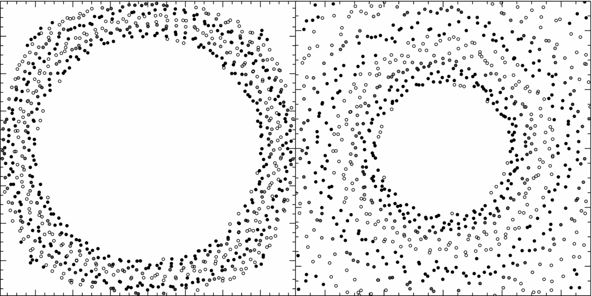
Interestingly and maybe surprisingly, the stretched glass performs relatively poorly, as shown in the middle panel of the bottom row. Even though the gravitational glass has excellent interpolation properties for uniform densities, this is not the case when stretched in a radial (or any other) direction. As was true for the lattice configurations, the stretching procedure tends to pronounce voids between planes that are perpendicular to the direction in which the stretching is applied. The glass does not have a uniform clear lattice structure but still tends to order particles along randomly oriented strings on a local level, as can be seen in the left panel of Figure 12. Thus, the stretching will preferably pick out those features that are perpendicular to our stretching direction, i.e., those inside shells. This leads to the wavy shell-like features in the right panel of Figure 12 which shows the stretched glass. In this particular example, the density deviations are on the order of 3%, which is significantly less than the lattice structures. However, with stronger stretching, these features will only become even more pronounced.
Unstretched (left) and stretched glass (right). Note the wavy shell-like structure in the stretched glass. To bring out this structure, particles are periodically coloured by their radius in the unstretched glass, which is then also applied to the stretched glass.
The WVT setup (bottom row, far-right panel) does not exhibit these features. Note how the level of noise for the adaptive setup is as low as for the uniform distribution. This is due to the fact that the WVT setup knows beforehand the desired resolution at each point in space, and is not a stretched version of a uniform distribution, allowing it to converge to the optimal solution in either case. We also note that this high level of interpolation accuracy does not depend on spherical symmetry as in the shell setup, which makes WVT much more versatile.
In summary, we find that stretched lattice configurations are not suitable for producing non-uniform particle distributions. Quaquaversal tiling and random configuration have even worse interpolation properties. The shell setup has acceptable levels of noise, but is restricted to spherical symmetry and the noise distribution is preferably along the radial direction. The stretched glass setup also introduces artefacts in shells which could lead to radial pulsations in an SPH simulation. The WVT setup has interpolation properties that are equivalent to the uniform distribution, which makes it the method of choice for adaptive resolution requirements. All other distributions should be relaxed into their equilibrium configuration prior to being used.
6.3 Particle noise
Another way of judging the characteristics of an SPH setup is to measure the particle noise inside a uniform distribution of particles within a uniform density distribution. In an ideal situation, all the pressure forces of individual particles cancel out, and the net force is 0 or very small compared to an individual force. Then, the contribution to the pressure force of an individual SPH particle i on another particle j is Monaghan (Reference Monaghan1992)
 $$\begin{equation}
{\text{d}v_{ij} \over \text{d}t}\propto -m_i {P_i \over \rho _i^2} \nabla _i W_{ij}.
\end{equation}$$
$$\begin{equation}
{\text{d}v_{ij} \over \text{d}t}\propto -m_i {P_i \over \rho _i^2} \nabla _i W_{ij}.
\end{equation}$$
For our test, we set up conditions such that the particle masses mi = 1, the average pressure  $\bar{P}_i=1$, and the average density $\bar{\rho }_i=1$. Thus, we expect a single particle to contribute |∇Wij| ≈ 0.08 on average to the acceleration term. Assuming Poisson noise, we thus expect the noise for a random configuration to be on the order of (N neigh)1/2 |∇Wij| = 0.64 for 64 neighbours.Footnote 2 Our random configuration yields a value of 0.60 ± 0.25 in our test setup, consistent with expectations. We will take this measured value of 0.6 as a reference point to measure the performance of the other setup methods in terms of ‘fractional Poisson noise’.
As expected, the uniform lattice configurations yield a perfect equilibrium down to machine precision. The quaquaversal tiling on the other hand shows very poor performance again, with a particle noise of about 30% the Poisson level, consistent with our findings in the density interpolation accuracy. Both the shell setup (3.9 ± 1.7%), the gravitational glass (3.1 ± 1.3%), and WVT (3.9 ± 1.7%) reduce the noise by an order of magnitude.
6.4 Summary
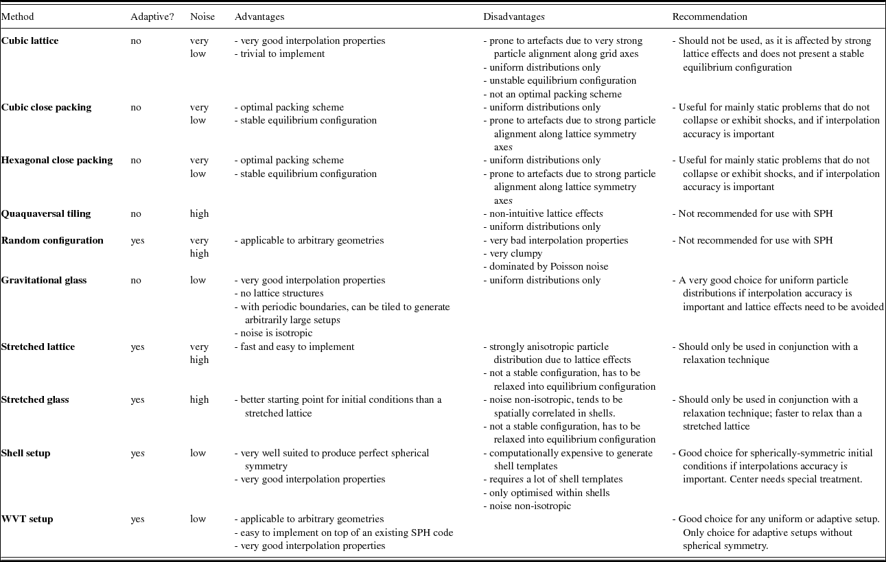
In Table 1, we summarise our findings about positive and negative characteristics of all considered setup methods for uniform particle distributions. We also provide recommendations for which method should be preferred in which situation.
Comparison of particle setup methods.
7 CONCLUSIONS
We have presented an extensive comparison of all particle setup methods currently employed in astrophysics that we are aware of. In particular, we review spatially uniform configurations such as a cubic lattice, CCP, HCP, quaquaversal tiling, and gravitational glasses. For spatially adaptive methods, we also include the random probability distribution, stretched lattice, stretched glass, and a concentrical shell setup. To the best of our knowledge, the stretched glass and concentrical shell setup have not been described in the literature before.
The main focus of our paper, however, is a new setup method based on WVTs. This new method allows for arbitrary spatial configurations of particles, which has not been possible before. We show that this new method is easy to implement on existing SPH codes and demonstrate its superior characteristics in several examples.
This method has now been used in a variety of astrophysics problems from core-collapse supernovae (Ellinger et al. Reference Ellinger, Young, Fryer and Rockefeller2012) to modelling binary interactions (Raskin et al. Reference Raskin, Timmes, Scannapieco, Diehl and Fryer2009, Reference Raskin, Timmes, Scannapieco, Diehl and Fryer2010; Fryer et al. Reference Fryer2010). Especially in doing binary interaction calculations comparing multiple techniques, using identical initial conditions is critical and these initial conditions tend to have complicated structures caused by tidal effects (e.g., Passy et al. Reference Passy2012).
ACKNOWLEDGMENTS
This work was carried out under the auspices of the National Nuclear Security Administration of the U.S. Department of Energy at Los Alamos National Laboratory under Contract No. DE-AC52-06NA25396. Three-dimensional images were created using the visit package developed at LLNL.