


1. Introduction
The large-scale structure evident in the matter distribution of the universe is predicted by the underlying cosmology. In the currently accepted $\Lambda$
CDM model, the universe began with the initial singularity, following which there was a period of rapid inflation. In the primordial field driving this inflation, there were quantum fluctuations, seeding small density variations in the early universe. The evolution and properties of these perturbations are related to the cosmological parameters, as the evolution of these perturbations in the otherwise homogeneous early universe are governed by various mechanisms, such as the collapse due to gravity, the expansion of the universe, and the propagation of the density fluctuations through the primordial medium. As such, one can use measurements of the large-scale structure inherent in galaxy surveys to test consistency with the values of the cosmological parameters derived from other methodologies, such as observing the Cosmic Microwave Background (CMB) (Planck Collaboration et al. Reference Collaboration2014a).
$\Lambda$
CDM model, the universe began with the initial singularity, following which there was a period of rapid inflation. In the primordial field driving this inflation, there were quantum fluctuations, seeding small density variations in the early universe. The evolution and properties of these perturbations are related to the cosmological parameters, as the evolution of these perturbations in the otherwise homogeneous early universe are governed by various mechanisms, such as the collapse due to gravity, the expansion of the universe, and the propagation of the density fluctuations through the primordial medium. As such, one can use measurements of the large-scale structure inherent in galaxy surveys to test consistency with the values of the cosmological parameters derived from other methodologies, such as observing the Cosmic Microwave Background (CMB) (Planck Collaboration et al. Reference Collaboration2014a).
In recent years there has been renewed interest in radio astronomy, and in particular low frequency radio astronomy, as instruments such as LOw-Frequency ARray (LOFAR) and the Murchison Widefield Array (MWA; Tingay et al. Reference Tingay2013; Wayth et al. Reference Wayth2018) perform large area sky surveys with unprecedented sensitivity. The Murchison Widefield Array (MWA) is a low-frequency radio telescope located at Inyarrimanha Ilgari Bundara/the Murchison Radio-astronomy Observatory, operating at a frequency range of over 72–231 MHz and is the instrument used in this study.
Prior studies have made successful measurements of the clustering inherent in the large-scale structure, through the angular correlation function (ACF) as well as other means. This has included studies with radio surveys, such as the work of Dolfi et al. (Reference Dolfi, Branchini, Bilicki, Balaguera-Antolnez, Prandoni and Pandit2019) using TIFR GMRT Sky Survey (TGSS; Intema et al. Reference Intema, Jagannathan, Mooley and Frail2017), the work of Blake & Wall (Reference Blake and Wall2002) using the NRAO VLA Sky Survey (NVSS; Condon et al. Reference Condon, Cotton, Greisen, Yin, Perley, Taylor and Broderick1998), and more recently that of Hale et al. (Reference Hale2024) using LOFAR Two-metre Sky Survey (LoTSS; Shimwell et al. Reference Shimwell2017) and that of Bahr-Kalus et al. (Reference Bahr-Kalus, Parkinson, Asorey, Camera, Hale and Qin2022) using Rapid ASKAP Continnum Survey (RACS; McConnell et al. Reference McConnell2020; Hale et al. Reference Hale2021). After accounting for survey and source specific factors such as sky coverage, resolution, and the bias inherent in the observed tracers of the matter distribution, these studies have shown consistency with the predictions of the $\Lambda$
CDM cosmological model.
$\Lambda$
CDM cosmological model.
In this study, the GLEAM-X, is used to measure the clustering of radio tracers, primarily active galactic nuclei (AGN), through measuring the ACF. In Section 2, the theoretical basis of the ACF is discussed. Following this, the methodology of this study shall be detailed in Section 3, with theoretical predictions discussed in Section 3.5. Covariance estimation is considered in Section 3.6. The results of this study and conclusion are summarised in Sections 4 and 5, respectively.
2. Theory
2.1. Power spectrum and cosmology
In the current $\Lambda$
CDM model of cosmology, the large-scale structure of the universe evident today evolved from the collapse of density fluctuations seeded in the very early universe (Peacock Reference Peacock1999). The theory of cosmological perturbations and their evolution is well developed (see e.g. Ma & Bertschinger Reference Ma and Bertschinger1995; Hawking Reference Hawking1966; Bardeen et al. Reference Bardeen, Bond, Kaiser and Szalay1986). Essentially, the initial density perturbations are generated during the early inflationary epoch, before their growth is affected by gravitational collapse, the expansion of the universe, and radiation pressure from the collapsing matter. To derive a theoretical consideration incorporating these factors, the boltzmann code Code for Anisotropies in the Microwave Background (CAMB) (Lewis, Challinor, & Lasenby Reference Lewis, Challinor and Lasenby2000) was used, to evolve the perturbation equations to provide theoretical predictions for the angular correlation function for a given cosmology: this is further discussed in Section 3.5.
$\Lambda$
CDM model of cosmology, the large-scale structure of the universe evident today evolved from the collapse of density fluctuations seeded in the very early universe (Peacock Reference Peacock1999). The theory of cosmological perturbations and their evolution is well developed (see e.g. Ma & Bertschinger Reference Ma and Bertschinger1995; Hawking Reference Hawking1966; Bardeen et al. Reference Bardeen, Bond, Kaiser and Szalay1986). Essentially, the initial density perturbations are generated during the early inflationary epoch, before their growth is affected by gravitational collapse, the expansion of the universe, and radiation pressure from the collapsing matter. To derive a theoretical consideration incorporating these factors, the boltzmann code Code for Anisotropies in the Microwave Background (CAMB) (Lewis, Challinor, & Lasenby Reference Lewis, Challinor and Lasenby2000) was used, to evolve the perturbation equations to provide theoretical predictions for the angular correlation function for a given cosmology: this is further discussed in Section 3.5.
2.2. Bias
In using radio sources to trace large-scale structure one must be mindful of the bias of various source populations in tracing the underlying matter density. In this case, bias refers to the degree to which the tracer population follows the matter distribution, specifically:
 \begin{equation} \delta_g=b\delta_m \,. \end{equation}
where $\delta_g$
is the perturbation in the galaxy density when compared to a homogeneous background,
$\delta_g$
is the perturbation in the galaxy density when compared to a homogeneous background, $\delta_m$
is the peturbation in the matter density, and b is the bias of the tracer. Models for the bias of varying galaxy types have been proposed in the literature, whether derived from N-Body simulations (Boylan-Kolchin et al. Reference Boylan-Kolchin, Springel, White, Jenkins and Lemson2009), analytically (Sheth, Mo, & Tormen Reference Sheth, Mo and Tormen2001; Catelan et al. Reference Catelan, Lucchin, Matarrese and Porciani1998), or empirically derived from observations (Bahr-Kalus et al. Reference Bahr-Kalus, Parkinson, Asorey, Camera, Hale and Qin2022). The most relevant of these in our case is that of Nusser & Tiwari (Reference Nusser and Tiwari2015), which was found by Siewert et al. (Reference Siewert2020) to fit their ACF, with LoTSS also being a low frequency continuum survey.
$\delta_m$
is the peturbation in the matter density, and b is the bias of the tracer. Models for the bias of varying galaxy types have been proposed in the literature, whether derived from N-Body simulations (Boylan-Kolchin et al. Reference Boylan-Kolchin, Springel, White, Jenkins and Lemson2009), analytically (Sheth, Mo, & Tormen Reference Sheth, Mo and Tormen2001; Catelan et al. Reference Catelan, Lucchin, Matarrese and Porciani1998), or empirically derived from observations (Bahr-Kalus et al. Reference Bahr-Kalus, Parkinson, Asorey, Camera, Hale and Qin2022). The most relevant of these in our case is that of Nusser & Tiwari (Reference Nusser and Tiwari2015), which was found by Siewert et al. (Reference Siewert2020) to fit their ACF, with LoTSS also being a low frequency continuum survey.
2.3. ACF and angular power spectrum (APS)
A radio survey such as GLEAM-X cannot be used to measure the 3-dimensional power spectrum directly, as the redshifts of the sources are unknown. The 2-dimensional angular power spectrum is observable however, being the projection of the 3-dimensional spectrum onto the celestial sphere. The density perturbations of equation 1 are related to the 3 dimensional power spectrum by
 \begin{equation} P\left(k\right) = \langle \delta_k\rangle^2 \end{equation}
where $\delta_k$
is the ensemble average power of wavemode k. The theoretical APS was derived, following (Bahr-Kalus et al. Reference Bahr-Kalus, Parkinson, Asorey, Camera, Hale and Qin2022):
$\delta_k$
is the ensemble average power of wavemode k. The theoretical APS was derived, following (Bahr-Kalus et al. Reference Bahr-Kalus, Parkinson, Asorey, Camera, Hale and Qin2022):
 \begin{equation} C_l=\frac{2}{\pi}\int dk k^2 P\left(k\right)\left[W_l\left(k\right)\right]^2 \,, \end{equation}
with
 \begin{equation} W_l\left(k\right)=\int dz n\left(z\right)b\left(z\right)D\left(z\right)j_l\left[k r\left(z\right)\right] \,. \end{equation}
where $C_l$
is the angular power spectrum coefficient of multipole l,
$C_l$
is the angular power spectrum coefficient of multipole l, $W_l\left(k\right)$
is the window function of wavenumber k,
$W_l\left(k\right)$
is the window function of wavenumber k, $b\left(z\right)$
is the bias of the tracers at redshift z,
$b\left(z\right)$
is the bias of the tracers at redshift z, $D\left(z\right)$
is the growth factor,
$D\left(z\right)$
is the growth factor, $n\left(z\right)$
is the number density,
$n\left(z\right)$
is the number density, $j_l$
is the Bessel function of order l, and
$j_l$
is the Bessel function of order l, and $r\left(z\right)$
is the co-moving distance to redshift z. The theoretical power spectrum
$r\left(z\right)$
is the co-moving distance to redshift z. The theoretical power spectrum $P\left(k\right)$
was derived using CAMB. The ACF
$P\left(k\right)$
was derived using CAMB. The ACF $w\left(\theta\right)$
was then calculated from this theoretical APS prediction using Equation (5), through a Legendre transform:
$w\left(\theta\right)$
was then calculated from this theoretical APS prediction using Equation (5), through a Legendre transform:
 \begin{equation} w\left(\theta\right)=\sum c_lP_l\left(\cos\left(\theta\right)\right) \,,\end{equation}
with
 \begin{equation} c_l=\frac{\left(2l+1\right)C_l}{4\pi} \,.\end{equation}
2.4. ACF
In essence, the ACF measures the clustering at each angular scale present in the data set, when compared to that expected if the tracer positions were random. Formally, following the form introduced by Peebles (Reference Peebles1980);
 \begin{equation} \delta P=N^2\delta \Omega_1 \delta \Omega_2\left(1+w\left(\theta\right)\right)\,, \end{equation}
where $w\left(\theta\right)$
is the ACF, pertaining to the probability
$w\left(\theta\right)$
is the ACF, pertaining to the probability $\delta P$
of two sources located in both solid angles
$\delta P$
of two sources located in both solid angles $\delta \Omega_1$
and
$\delta \Omega_1$
and $\delta \Omega_2$
separated by an angle
$\delta \Omega_2$
separated by an angle $\theta$
. Thus, the ACF formally relates to the probability overdensity, indicative of the source clustering: in the trivial case where w is uniformly zero, one can see that this reduces to the source density multiplied by the area.
$\theta$
. Thus, the ACF formally relates to the probability overdensity, indicative of the source clustering: in the trivial case where w is uniformly zero, one can see that this reduces to the source density multiplied by the area.
Various estimators for the ACF have been proposed, among the most intuitive being that derived from Monte Carlo integration (Peebles Reference Peebles1980; Landy & Szalay Reference Landy and Szalay1993):
 \begin{equation} w\left(\theta \right)=DD/RR-1 \,. \end{equation}
In this work, that of Landy & Szalay (Reference Landy and Szalay1993) is used, due to the lower variance (Blake & Wall Reference Blake and Wall2002; Landy & Szalay Reference Landy and Szalay1993):
 \begin{equation} w\left(\theta\right)=\frac{DD}{RR}-\frac{2DR}{RR}+1 \,, \end{equation}
where DD is the number of galaxy pairs in the sample at an angular distance $ \theta\Longrightarrow\theta+\delta\theta\, $
, RR is the number in a random sample, and DR is the number of pairs found between the catalogue and random sources.
$ \theta\Longrightarrow\theta+\delta\theta\, $
, RR is the number in a random sample, and DR is the number of pairs found between the catalogue and random sources.
3. Methodology
3.1. Data
The GLEAM-X survey was performed with the Murchison Widefield Array (MWA; Tingay et al. Reference Tingay2013; Wayth et al. Reference Wayth2018), surveying the sky south of $+30$
degrees declination. The survey has observed the frequency range of 72–231 MHz, and the final data will have a resolution varying from 2′ to 45′′, with a resolution of approximately 45′′ in the 170–231 MHz image, used for source-finding. The first data release from the GLEAM-X survey was produced in 2022, covering 4 h
$+30$
degrees declination. The survey has observed the frequency range of 72–231 MHz, and the final data will have a resolution varying from 2′ to 45′′, with a resolution of approximately 45′′ in the 170–231 MHz image, used for source-finding. The first data release from the GLEAM-X survey was produced in 2022, covering 4 h $\leq$
RA
$\leq$
RA $\leq$
13 h, and Declination range
$\leq$
13 h, and Declination range $-32.7^\circ$
to
$-32.7^\circ$
to $-20.7^\circ$
(Hurley-Walker et al. Reference Hurley-Walker2022). Data release 2 will cover 20 h40 m
$-20.7^\circ$
(Hurley-Walker et al. Reference Hurley-Walker2022). Data release 2 will cover 20 h40 m $\leq$
RA
$\leq$
RA $\leq$
6 h40 m, -90
$\leq$
6 h40 m, -90 $\leq$
Dec
$\leq$
Dec $\leq$
+30 (Ross et al. Reference Ross2024).
$\leq$
+30 (Ross et al. Reference Ross2024).
The ACF was calculated from a subset of the GLEAM-X data. The usable data was reduced by highly sporadic noise properties near the edges of the image, leading to variations in source density. As discussed by Blake & Wall (Reference Blake and Wall2002), due to the dependence of the galaxy data pairings on the local source density, i.e on the amount of clustering, differing with that of the randoms, which is dependent on the global density, the ACF can be artificially increased. As such, a mask was applied to the data, to excise these regions from the image, resulting in sections between RA $21^h 4^m$
to
$21^h 4^m$
to $6^h 24^m$
, and Dec
$6^h 24^m$
, and Dec $-40^\circ$
to
$-40^\circ$
to $0^\circ$
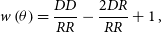
being used. This is shown in Fig. 1, and shall hereby be referred to as GLEAM-X Data Subset (GXDS). This region contains 362 944 sources, found in the source-finding image by the AEGEAN source finding package (Hancock, Trott & Hurley-Walker Reference Hancock, Trott and Hurley-Walker2018) as part of GLEAM-X processing and has a mean rms value of
$0^\circ$
being used. This is shown in Fig. 1, and shall hereby be referred to as GLEAM-X Data Subset (GXDS). This region contains 362 944 sources, found in the source-finding image by the AEGEAN source finding package (Hancock, Trott & Hurley-Walker Reference Hancock, Trott and Hurley-Walker2018) as part of GLEAM-X processing and has a mean rms value of $1\,\mathrm{mJy\ beam^{-1}}$
. AEGEAN uses a novel source finding technique, namely priorised fitting, whereby the location of a source is determined in the source finding image, and then used at lower frequencies to inform where the source should be (Hurley-Walker et al. Reference Hurley-Walker2022).
$1\,\mathrm{mJy\ beam^{-1}}$
. AEGEAN uses a novel source finding technique, namely priorised fitting, whereby the location of a source is determined in the source finding image, and then used at lower frequencies to inform where the source should be (Hurley-Walker et al. Reference Hurley-Walker2022).
A view of the GXDS region, highlighted in the white box, and the rms values. The GLEAM-X DR2 region is shown in the black dashed line.
The completeness of GLEAM-X DR2 is discussed by Ross et al. (Reference Ross2024). The survey is approximately 90% complete in this region for a flux density level of 10 mJy. As such, a flux density cut of 10 mJy was applied to both the randoms and data, the cut being performed at the source-finding image central frequency of 200 MHz.
3.2. Source counts
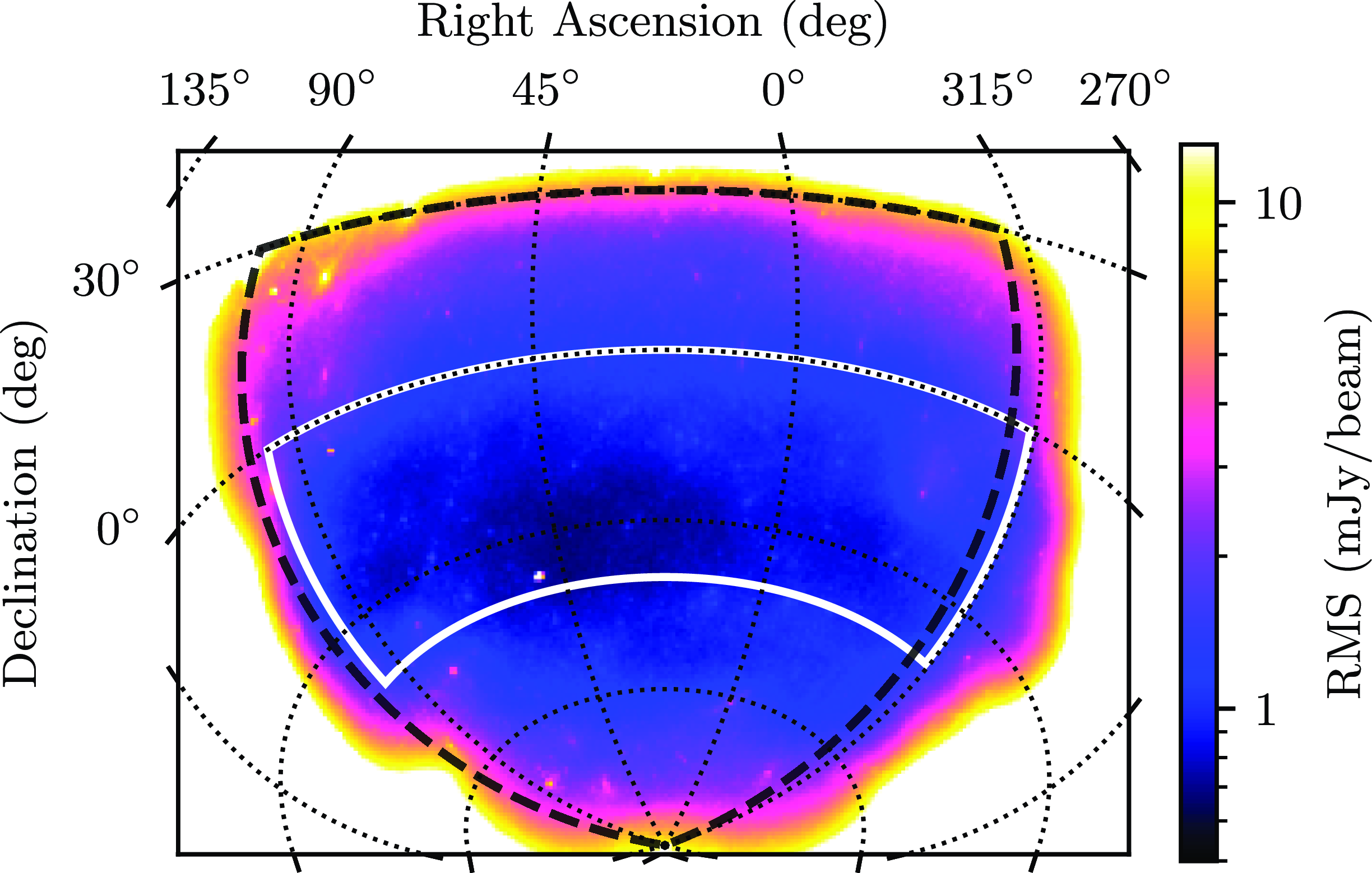
The GLEAM-X GXDS differential source counts are shown in Fig. 2. This uses the GXDS region defined in Section 3.1, with 200 610 sources after flux density cutting. One can see good agreement with other surveys, namely that of the 151-MHz 7C survey (Hales et al. Reference Hales, Riley, Waldram, Warner and Baldwin2007), 200-MHz counts from the GaLactic and Extragalactic All-sky Murchison Widefield Array survey (GLEAM) survey (Franzen et al. Reference Franzen2016), and source counts from Giant Meterwave Radio Telescope (GMRT) observations of the Boötes field (Intema et al. Reference Intema, van Weeren, Röttgering and Lal2011). It is also evident from the counts that the survey drops considerably in completeness below 10 mJy. This is reflected in a flux density cut applied to the data (see Section 3.1) before measurements of the source counts and ACF were made. The source counts are tabulated in Appendix 5
The normalised Euclidean source counts of the GXDS region, compared to other surveys, namely the the 151-MHz 7C survey (Hales et al. Reference Hales, Riley, Waldram, Warner and Baldwin2007), 200-MHz counts from the GLEAM survey (Franzen et al. Reference Franzen2016), and source counts from GMRT observations of the Boötes field (Intema et al. Reference Intema, van Weeren, Röttgering and Lal2011). The source counts have not been corrected for frequency scaling.
3.3. Angular correlation function
Following this, random sources were generated, to compare the clustering to that present in the data. As well as a random position, these sources were assigned a flux density, this value being derived from the n(s) distribution for the GLEAM-X data. In an effort to replicate the effect of noise on surface density in the remaining image, the random sources were retained if the flux density, which when a normally distributed noise component was added, was 5 $\sigma$
above the noise, as per the process used in GLEAM-X source finding. A further flux density cut of 10 mJy was made, to ensure the uniformity of the source density, as discussed in Section 3.1.
$\sigma$
above the noise, as per the process used in GLEAM-X source finding. A further flux density cut of 10 mJy was made, to ensure the uniformity of the source density, as discussed in Section 3.1.
The ACF of the resulting data was then calculated. The measurement of the pairs at a given angular separation was done using the TreeCorr (Jarvis, Bernstein, & Jain Reference Jarvis, Bernstein and Jain2004) package, for both the GLEAM-X galaxies and the generated random catalogues.
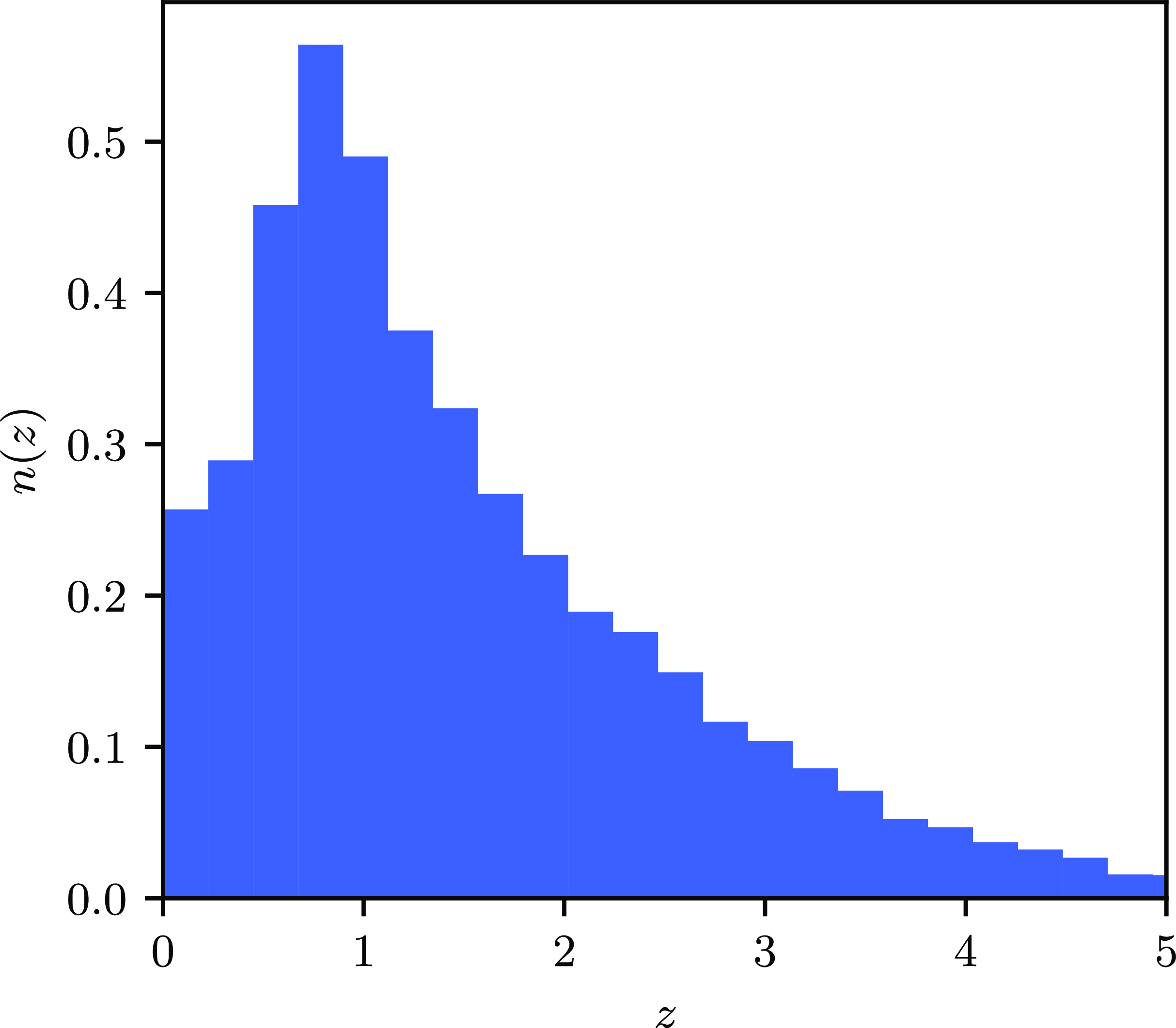
3.4. Window function, redshift distribution and n(z)
In translating the 3-dimensional clustering prediction to the observed ACF, one must assume some information about how the sources are clustered in redshift space. To make an informed prediction, the European SKA Design Study Simulated Skies (SKADS; Wilman et al. Reference Wilman2008) simulations were used: these simulations were conducted to provide a dataset resembling that which may eventuate from the Square Kilometre Array (SKA; Dewdney et al. Reference Dewdney, Hall, Schilizzi and Lazio2009), so astronomers could test science cases with a realistic dataset. A flux density cut of 10 mJy was applied to the European SKA Design Study Simulated Skies (SKADS) estimate, scaled to the SKADS frequency of 1.4 GHz, and the redshift distribution of the resulting sources was chosen to approximate that in GXDS. The $n\left(z\right)$
distribution is shown in Fig. 3.
$n\left(z\right)$
distribution is shown in Fig. 3.
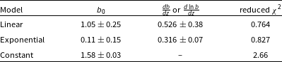
3.5. Theoretical estimation and bias fitting
As mentioned above, the observed angular power spectrum and ACF are related to the fundamental parameters of our universe. As an intent of our work is to see if the measurements made using the GLEAM-X data are consistent with the currently accepted $\Lambda$
CDM cosmological values, summarised in Table 1. We set the default cosmology for theoretical predictions to these values. Indeed, degeneracy in the computations involving bias and n(z), as demonstrated in equation 4, mean that we would be unable to measure the values exclusively from the GLEAM-X data without assuming the value of arbitrarily chosen parameters. The chosen values, from Planck Collaboration et al. (Reference Collaboration2020), were used to generate a theoretical power spectrum and correlation function, thereby allowing theoretical comparison with the observed data.
$\Lambda$
CDM cosmological values, summarised in Table 1. We set the default cosmology for theoretical predictions to these values. Indeed, degeneracy in the computations involving bias and n(z), as demonstrated in equation 4, mean that we would be unable to measure the values exclusively from the GLEAM-X data without assuming the value of arbitrarily chosen parameters. The chosen values, from Planck Collaboration et al. (Reference Collaboration2020), were used to generate a theoretical power spectrum and correlation function, thereby allowing theoretical comparison with the observed data.
Attempts were made in this work to derive the bias (see Section 2.2) of the source population, primarily AGN in GLEAM-X (Franzen et al. Reference Franzen, Vernstrom, Jackson, Hurley-Walker, Ekers, Heald, Seymour and White2019), and check consistency with various theoretically motivated and parametric models (Siewert et al. Reference Siewert2020; Bahr-Kalus et al. Reference Bahr-Kalus, Parkinson, Asorey, Camera, Hale and Qin2022; Blake, Ferreira, & Borrill Reference Blake, Ferreira and Borrill2004). To do this, the ACF and angular power spectrum, assuming best-fitting Planck cosmology, were theoretically estimated with multiple bias models, and the model that best fit the observational data identified. The models used are listed in Table 2.
The cosmological parameters used in this analysis.
The SKADS approximated distribution of GLEAM-X redshifts, as discussed in Section 3.4.
The best fitting bias fits for the GLEAM-X ACF, plotted in Fig. 6.
3.6. Covariance estimation
In estimating the covariance of the angular power spectrum, including both that due to cosmic variance and statistical variance, three techniques were used: two internal and one external. The covariance matrix was calculated analytically from the data, using the Jackknife methodology of Norberg et al. (Reference Norberg and Baugh2009), and externally through the variance of generated mock galaxy catalogues. This was necessary due to the effects of cosmic variance not being measured by internal covariance estimators, such as that calculated analytically (Bahr-Kalus et al. Reference Bahr-Kalus, Parkinson, Asorey, Camera, Hale and Qin2022; Eisenstein & Zaldarriaga Reference Eisenstein and Zaldarriaga2001).
3.6.1. Jackknife estimation
The first method of estimating the covariance matrix was by ‘jackknife’ estimation (Norberg et al. Reference Norberg and Baugh2009). 50 subsamples of the healpix cells to which the sky distribution was binned were drawn, each sample consisting of non adjacent healpix cells exclusive to that subsample. The ACF of the sky excluding each sub-sample was then calculated for all subsamples. The overall covariance matrix was then estimated as:
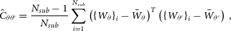 \begin{equation} \hat{C}_{\theta\theta^{\prime}}=\frac{N_{sub}-1}{N_{sub}}\sum_{i=1}^{N_{sub}}\left(\left\{W_{\theta}\right\}_i-{\bar{W}}_\theta\right)^{T}\left(\left\{W_{\theta^{\prime}}\right\}_i-{\bar{W}}_{\theta^{\prime}}\right) \,, \end{equation}
with $W_\theta$
the correlation function at angle
$W_\theta$
the correlation function at angle $\theta$
, and:
$\theta$
, and:
 \begin{equation} \bar{W}_\theta=\frac{1}{N_{sub}}\sum_{i=1}^{N_{mock}}\left\{W_{\theta}\right\}_i \,. \end{equation}
3.6.2. Analytic covariance
The covariance matrix was also estimated analytically following Crocce, Cabré, & Gaztañaga (Reference Crocce, Cabré and Gaztañaga2011). That is, the analytic covariance between two angles $\theta$
and
$\theta$
and $\theta^{\prime}$
is represented by:
$\theta^{\prime}$
is represented by:
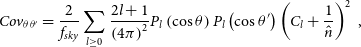 \begin{equation} Cov_{\theta\theta^{\prime}}=\frac{2}{f_{sky}}\sum_{l\geq0}\frac{2l+1}{\left(4\pi\right)^2}P_l\left(\cos{\theta}\right)P_l\left(\cos{\theta^{\prime}}\right)\left(C_l+\frac{1}{\hat{n}}\right)^2 \,, \end{equation}
with $C_l$
estimated as per equation 3,
$C_l$
estimated as per equation 3, $\hat{n}$
the source density per steradian, and
$\hat{n}$
the source density per steradian, and $f_{sky}$
the fraction of sky covered by the survey.
$f_{sky}$
the fraction of sky covered by the survey.
3.6.3. Covariance of mock samples
In order to quantify the effect of cosmic variance and validate the covariance matrix, the covariance was estimated from mock galaxy catalogues, generated from the same underlying cosmology as that measured by Planck Collaboration et al. (Reference Collaboration2014b), and consistent with the GLEAM-X angular power spectrum and ACFs measured in this work. The sample covariance of the mock realisations is calculated as (Bahr-Kalus et al. Reference Bahr-Kalus, Parkinson, Asorey, Camera, Hale and Qin2022):
 \begin{equation} \hat{C}_{\theta\theta^{\prime}}=\frac{1}{N_{mock}-1}\sum_{i=1}^{N_{mock}}\left(\left\{W_{\theta}\right\}_i-{\bar{W}}_\theta\right)^{T}\left(\left\{W_{\theta^{\prime}}\right\}_i-{\bar{W}}_{\theta^{\prime}}\right) \,. \end{equation}
In generating these mock samples, the Generator for large-scale Structure (GLASS; Tessore et al. Reference Tessore, Loureiro, Joachimi, von Wietersheim-Kramsta and Jeffrey2023) software package was used to generate mock catalogues. Generator for large-scale Structure builds light cones in an iterative manner, given an assumed underlying cosmology, with values in this paper set to those detailed by Planck Collaboration et al. (Reference Collaboration2020), referenced in Table 1. GLASS uses a hybrid of statistical and physical models, log-normal realisations of the Gaussian field, and other relations to produce accurate realisations in reasonable timeframes. We used 500 mocks in our analysis, generated with a maximum multipole l of 24 564. The covariance matrices are discussed in Section 4.5.
4. Results
4.1. ACF
The ACF derived from the GLEAM-X is displayed in Fig. 4 with errors derived from the Jackknife covariance matrix (see Section 3.6.1). The form of the ACF resembles that of prior results; in particular, it displays the double power law morphology of the ACF produced by Blake & Wall (Reference Blake and Wall2002): at a similar angular scale to Blake & Wall (Reference Blake and Wall2002) we see an increase in the slope of the correlation function. In Blake & Wall (Reference Blake and Wall2002) this is attributed to multiple-component sources: we attribute this to similar features, as discussed in Section 4.4.
The ACF computed with various surveys. The crosses show that computed in this work with the GXDS survey data, whilst those from the work of Blake & Wall (Reference Blake and Wall2002) using the NRAO VLA Sky Survey (NVSS; Condon et al. Reference Condon, Cotton, Greisen, Yin, Perley, Taylor and Broderick1998), and more recently that of Hale et al. (Reference Hale2024) using LOFAR Two-metre Sky Survey (LoTSS; Shimwell et al. Reference Shimwell2017). Also shown is a result by Connolly et al. (Reference Connolly2002) using the Sloan Digital Sky Survey (SDSS; York et al. Reference York2000). Note that the three fits displayed make use of Limber’s approximation (Limber Reference Limber1953), and model the ACF as a power law.
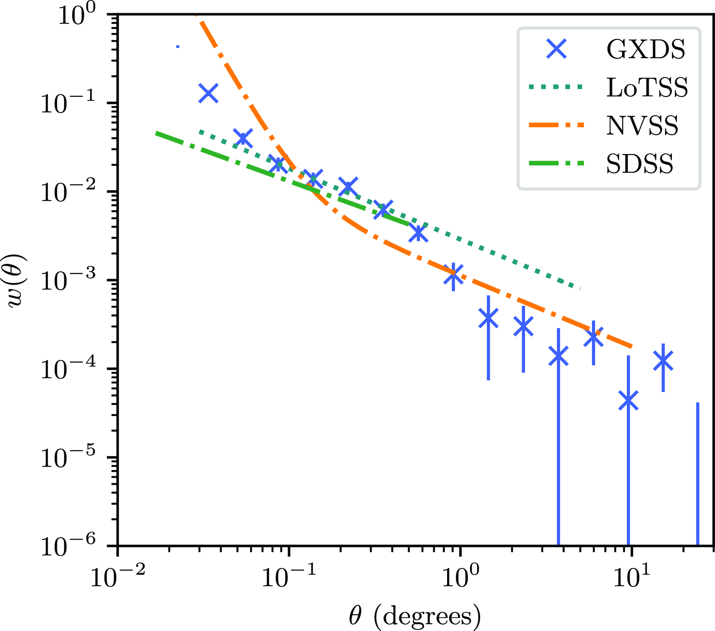
It is important to note that the fitting of the ACF as a power law, as in works by Blake & Wall (Reference Blake and Wall2002) and Hale et al. (Reference Hale2024) relies on Limber’s approximation Limber (Reference Limber1953), which is only applicable for small angular scales. Below the scale of 1 $^\circ$
we see excellent agreement with the ACF presented by Hale et al. (Reference Hale2024).
$^\circ$
we see excellent agreement with the ACF presented by Hale et al. (Reference Hale2024).
One also sees similar cosmological slope (i.e the slope of the power-law component not due to multiple component sources, seen at angular scales of about $~0.1$
degrees) to Hale et al. (Reference Hale2024) and Connolly et al. (Reference Connolly2002), but a difference in amplitude, and an overall curvature at higher angular scales. The amplitude of the ACF is dependent on flux density, luminosity and source type (Hale et al. Reference Hale2024), and as this differs for the different surveys, we would not expect this to match exactly. This is further discussed in Section 4.3.
$~0.1$
degrees) to Hale et al. (Reference Hale2024) and Connolly et al. (Reference Connolly2002), but a difference in amplitude, and an overall curvature at higher angular scales. The amplitude of the ACF is dependent on flux density, luminosity and source type (Hale et al. Reference Hale2024), and as this differs for the different surveys, we would not expect this to match exactly. This is further discussed in Section 4.3.
4.2. Systematic effects
As per prior studies such as that by Hale et al. (Reference Hale2024), systematic effects in the data can give the measure of spurious clustering in the resulting ACF. The GLEAM-X data used in this work has the potential to be affected by three effects, namely flux density scaling, calibration errors and ionospheric effects that could smear out the sources, and primary beam dependent effects. These are addressed in turn.
4.2.1. Flux density scaling
The flux density scale for GLEAM-X was computed using a model from the precursor survey GLEAM. GLEAM in turn has a flux density scale derived from the NRAO VLA Sky Survey (NVSS), Sydney University Molonglo Sky Survey (SUMSS; Bock, Large, & Sadler Reference Bock, Large and Sadler1999), and the Very Large Array Low-frequency Sky Survey Redux (VLSSr; Lane et al. Reference Lane, Cotton, van Velzen, Clarke, Kassim, Helmboldt, Lazio and Cohen2014). As detailed by Hurley-Walker et al. (Reference Hurley-Walker2017), this leads to an internal flux density scale that is free of Declination-dependent effects down to a Declination of $-72^\circ$
, which was also tested with independently-calibrated VLA observations of various well-known calibrator sources. Both GLEAM and GLEAM-X processing are performed in drift scans with very large primary beam overlaps, leading to minimal variation in the flux density scale with Right Ascension. The sub-band channels are processed independently using the same methods, and the final radio source spectra derived from these measurements are consistent with those expected from other studies i.e. a median spectral index of
$-72^\circ$
, which was also tested with independently-calibrated VLA observations of various well-known calibrator sources. Both GLEAM and GLEAM-X processing are performed in drift scans with very large primary beam overlaps, leading to minimal variation in the flux density scale with Right Ascension. The sub-band channels are processed independently using the same methods, and the final radio source spectra derived from these measurements are consistent with those expected from other studies i.e. a median spectral index of $\alpha=-0.83$
, where flux density
$\alpha=-0.83$
, where flux density $S\propto\nu^\alpha$
, for bright, isolated AGN (Hurley-Walker et al. Reference Hurley-Walker2017, Reference Hurley-Walker2022). We therefore have no cause to suspect any issues with the flux density scale that could cause any systematics in the measured clustering.
$S\propto\nu^\alpha$
, for bright, isolated AGN (Hurley-Walker et al. Reference Hurley-Walker2017, Reference Hurley-Walker2022). We therefore have no cause to suspect any issues with the flux density scale that could cause any systematics in the measured clustering.
4.2.2. Smearing
A potential issue in the dataset that has affected other results (Hale et al. Reference Hale2024), is that of smearing, namely sources being altered in dimension such that the peak flux density is reduced, and the source subsequently not detected. To gauge whether this is an issue for GLEAM-X, we consulted the rms maps for the region considered, and reviewed the procedures that went into making the GLEAM-X mosaics, as detailed by Ross et al. (Reference Ross2024). Briefly, a catalogue of sparse, unresolved, and high signal-to-noise sources from NVSS and Sydney University Molonglo Sky Survey (SUMSS) is constructed, and the ratio of the integrated to peak flux density for those sources in GLEAM-X is calculated. A mean greater than or equal to $1.1$
or a standard deviation greater than or equal to
$1.1$
or a standard deviation greater than or equal to $0.125$
of
$0.125$
of $S_{int}/S_{peak}$
saw the observation flagged and not included in the final mosaics. Furthermore, in constructing the GLEAM-X mosaics, ionospheric corrections were applied to the positions of the sources, with the catalogue of NVSS and SUMSS sources used to derive a model of position shifts (Hurley-Walker et al. Reference Hurley-Walker2022). These were applied to every image before mosaicing. Only unresolved, single component sources were used in these corrections. Finally, a 5 sigma applied to the data and randoms should ensure that any smearing remains minimal.
$S_{int}/S_{peak}$
saw the observation flagged and not included in the final mosaics. Furthermore, in constructing the GLEAM-X mosaics, ionospheric corrections were applied to the positions of the sources, with the catalogue of NVSS and SUMSS sources used to derive a model of position shifts (Hurley-Walker et al. Reference Hurley-Walker2022). These were applied to every image before mosaicing. Only unresolved, single component sources were used in these corrections. Finally, a 5 sigma applied to the data and randoms should ensure that any smearing remains minimal.
4.2.3. Primary beam effects and other effects
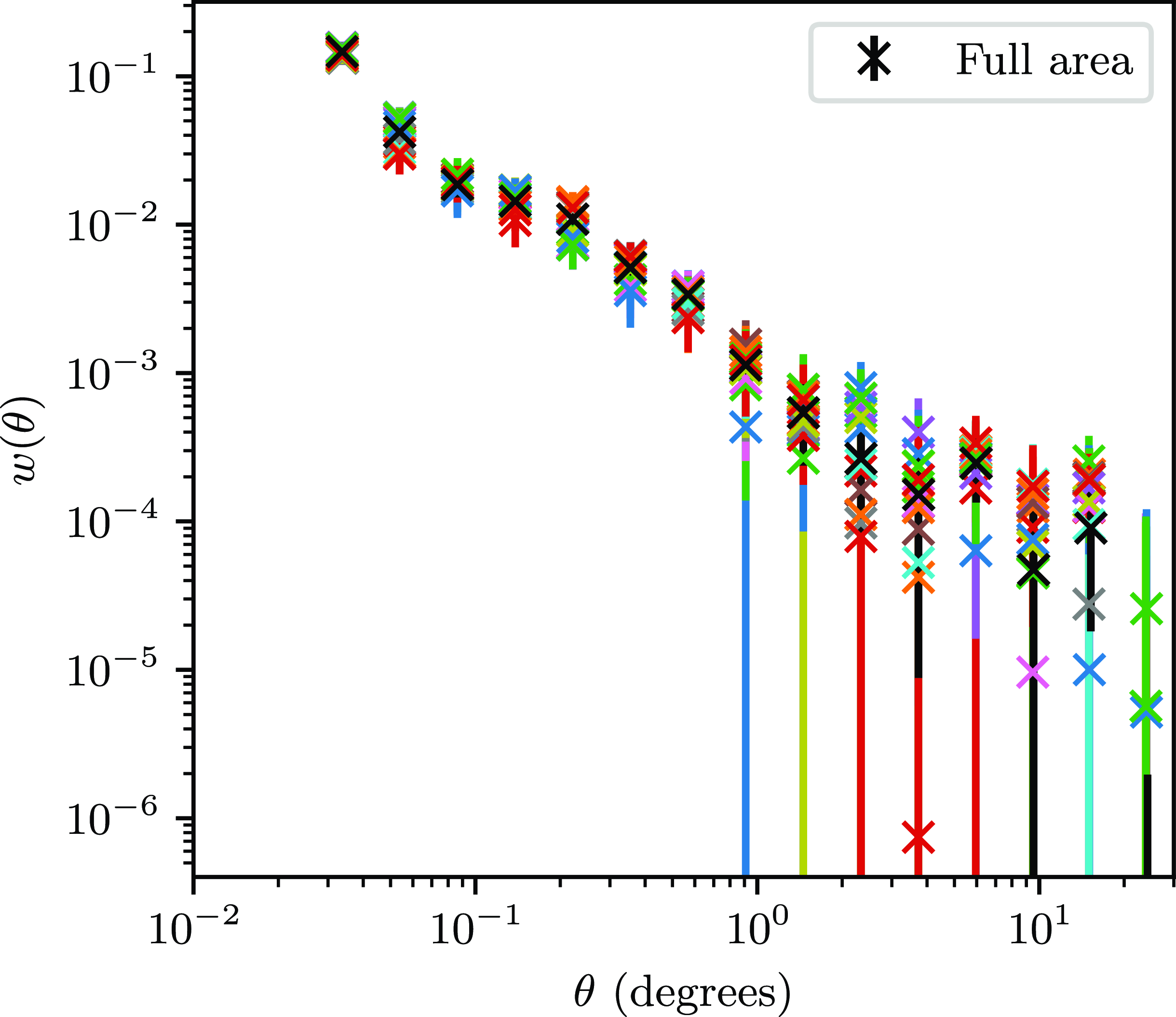
To further see if factors such as flux density scaling and position dependent affects contribute to the uncertainty of the ACF, the area used in this study was divided into 14 regions, each square in RA and Dec and 20 degrees on a side, and the ACF calculated from each region. This is presented in Fig. 5, with the ACF’s presented separately in Appendix 2, Fig. A1. Particularly on the small scales, one can see that the calculated ACF is similar for all regions, diverging somewhat at scales over 10 degrees. However, the variation is within the errors from the full area. There does not seem to be an observed trend with either RA or Dec.
The ACF calculated for each sub-region of the GXDS dataset.

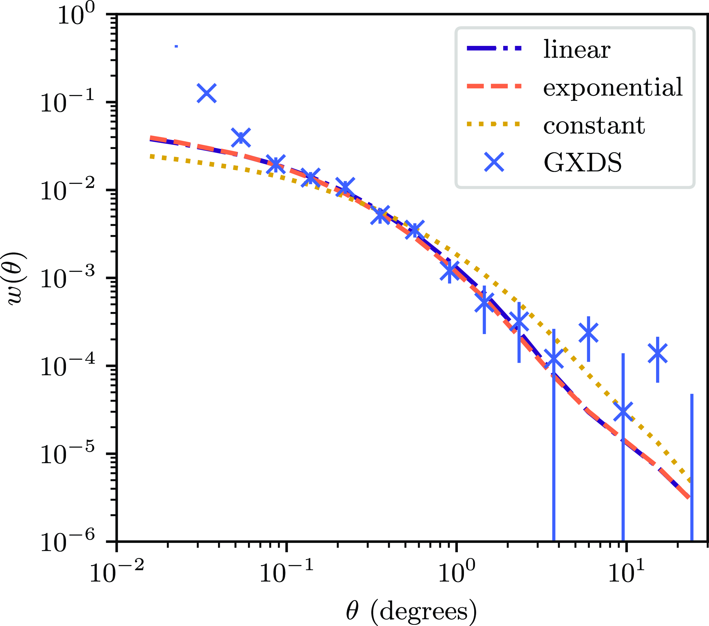
The theoretical ACF derived from various bias fits, with the observational ACF for comparison, as discussed in Section 4.3. The plotted data is identical to that in Fig. 4.
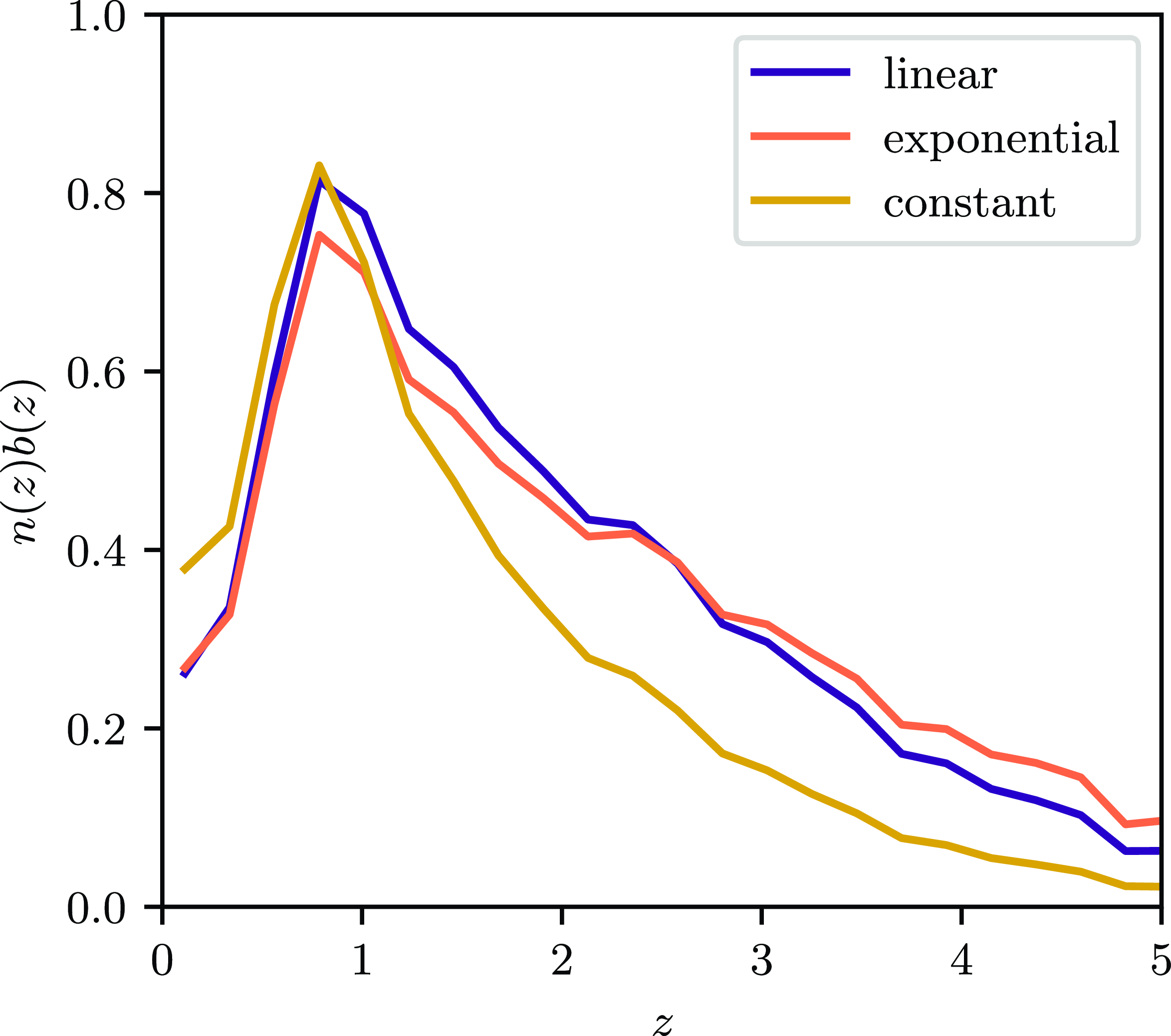
 $n\left(z\right)b\left(z\right)$
for the various best fit bias fits described in Section 4.3. The three bias fits, namely linear, exponential, and constant, are of the form
$n\left(z\right)b\left(z\right)$
for the various best fit bias fits described in Section 4.3. The three bias fits, namely linear, exponential, and constant, are of the form $b\left(z\right)=a\times, z+b_0$
,
$b\left(z\right)=a\times, z+b_0$
, $b\left(z\right)=a\times e^{b_0\times z}$
and
$b\left(z\right)=a\times e^{b_0\times z}$
and $b\left(z\right)=b_0$
respectively, with
$b\left(z\right)=b_0$
respectively, with $n\left(z\right)$
derived from SKADS.
$n\left(z\right)$
derived from SKADS.
The variation about the ACF calculated using the full GXDS region is significant for scales over approximately $1^\circ$
. The jackknife covariance matrix was calculated using 50 patches, and as such the sky area covered in each patch will be smaller, however variation in source density over different sky patches could still significantly contribute to the jackknife covariance at larger scales.
$1^\circ$
. The jackknife covariance matrix was calculated using 50 patches, and as such the sky area covered in each patch will be smaller, however variation in source density over different sky patches could still significantly contribute to the jackknife covariance at larger scales.
4.3. Bias fits
As discussed in Section 2.2, when using discrete tracers of the underlying matter distribution, one needs to be mindful of their bias. An attempt was made in this work to derive the bias of the AGN observed by the GLEAM-X survey. Four different bias models were fitted. The first was the bias model discussed by Nusser & Tiwari (Reference Nusser and Tiwari2015) and used in Siewert et al. (Reference Siewert2020):
 \begin{equation} b\left(z\right)=1.6+0.85z+0.33z^2 \,, \end{equation}
and three parametric models, namely:
 \begin{equation} b\left(z\right)=az+b_0 \,, \end{equation}
 \begin{equation} b\left(z\right)=ae^{b_0\times z} \,, \end{equation}
 \begin{equation} b\left(z\right)=b_0 \,. \end{equation}
The best-fitting values of the parametric models are displayed in Table 2, and plotted in Fig. 6. The corresponding theoretical ACF’s are plotted in Fig. 7, and the corresponding $n (z) b (z)$
for each bias model in Fig. 8. The bias models were fitted excluding the first 4 data points, covering scales to
$n (z) b (z)$
for each bias model in Fig. 8. The bias models were fitted excluding the first 4 data points, covering scales to $~0.1^\circ$
, for the uptick in the gradient of the ACF evident in these points can be attributed to multiple component sources, as discussed in Section 4.4.
$~0.1^\circ$
, for the uptick in the gradient of the ACF evident in these points can be attributed to multiple component sources, as discussed in Section 4.4.
We find that the model of Nusser & Tiwari (Reference Nusser and Tiwari2015) is not consistent with our ACF. Of course, given the degeneracy for the $n\left(z\right)$
and the
$n\left(z\right)$
and the $b\left(z\right)$
distributions in computing the ACF, and the fact that the redshift distribution of the GLEAM-X galaxies was approximated from SKADS, this may simply be representative of our redshift distribution being uncertain.
$b\left(z\right)$
distributions in computing the ACF, and the fact that the redshift distribution of the GLEAM-X galaxies was approximated from SKADS, this may simply be representative of our redshift distribution being uncertain.
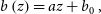
The three correlation matrices for the analysis. That computed by the jackknife methodology in Section 3.6.1 is on the left, the centre figure concerns the theoretical methodology discussed in Section 3.5, and the right figure depicts that computed using the sample variance methodology in Section 3.6.3.
4.4. Multiple component sources
When viewing the ACF derived from the GLEAM-X survey, one can see an increase in the gradient at angular separations lower than $~0.1$
degrees. This phenomenon is seen in prior studies, such as that by Blake & Wall (Reference Blake and Wall2002), and is representative of sources with multiple components being included in the analysis, spuriously enhancing the clustering. Given GLEAM-X has the same resolution as the NVSS, the survey used in Blake & Wall (Reference Blake and Wall2002), it is reassuring we see a similar feature.
$~0.1$
degrees. This phenomenon is seen in prior studies, such as that by Blake & Wall (Reference Blake and Wall2002), and is representative of sources with multiple components being included in the analysis, spuriously enhancing the clustering. Given GLEAM-X has the same resolution as the NVSS, the survey used in Blake & Wall (Reference Blake and Wall2002), it is reassuring we see a similar feature.
When compared to Blake & Wall (Reference Blake and Wall2002), one can see the gradient of the ACF caused by the multiple component sources is lower in our study. However, when we re-compute the ACF after a flux density cut of 50mJy, consistent with the Blake & Wall (Reference Blake and Wall2002) study with an assumed spectral index of $-0.83$
, we recover the same ACF as Blake & Wall (Reference Blake and Wall2002). With the extra sensitivity of the GLEAM-X survey, we are detecting fainter sources which are less resolved, thus decreasing the proportion of sources that have multiple components, and reducing the gradient of our ACF at scales below
$-0.83$
, we recover the same ACF as Blake & Wall (Reference Blake and Wall2002). With the extra sensitivity of the GLEAM-X survey, we are detecting fainter sources which are less resolved, thus decreasing the proportion of sources that have multiple components, and reducing the gradient of our ACF at scales below $0.1 ^\circ$
.
$0.1 ^\circ$
.
4.5. Covariance measures
The correlation matrices for the analysis are shown in Fig. 9. As prefaced in Section 3.6, this allows the estimation of the contributions of cosmic and statistical variance to the errors of the measured ACF.
In viewing the jackknife correlation matrix estimate in Fig. 9, one is struck by two evident features. The first is the expected higher amplitude on the diagonal, expected as the variance of bins will be higher than the covariance of one bin with a different bin. The second feature is the large amount of correlation at the larger angular scales, from approximately $1^\circ$
. This can be attributed to two effects, both limiting the amount of independent samples at higher angular scales. The first is the limited sky coverage, imposed by our survey mask, and the second is the source density, resulting in their being less pairs to sample from. The first of these is equivalent to the approximation, present in multiple prior studies (Eisenstein & Zaldarriaga Reference Eisenstein and Zaldarriaga2001; Scott, Srednicki, & White Reference Scott, Srednicki and White1994) that the error in the angular power spectrum scales with
$1^\circ$
. This can be attributed to two effects, both limiting the amount of independent samples at higher angular scales. The first is the limited sky coverage, imposed by our survey mask, and the second is the source density, resulting in their being less pairs to sample from. The first of these is equivalent to the approximation, present in multiple prior studies (Eisenstein & Zaldarriaga Reference Eisenstein and Zaldarriaga2001; Scott, Srednicki, & White Reference Scott, Srednicki and White1994) that the error in the angular power spectrum scales with $\frac{1}{f_{sky}}$
.
$\frac{1}{f_{sky}}$
.
Interestingly, the theoretical correlation matrix in Fig. 9b, does not show the same large correlation at high angular scales, however at small scales the theoretical correlation matrix shows an increase in the relative cross-correlation of the measurements. The lack of the large-scale correlations is not surprising, as the theoretical matrix computations do not take into account the shape of the survey mask. The matrix has far lower off-diagonal components than either the jackknife or sample variance matrix, differing by several orders of magnitude, indicating that these off-diagonal elements are greatly affected by survey related matters such as the survey mask, as well as cosmic variance.
The final of the three correlation matrices, that relating to the sample variance methodology, shows a mixture of two features and is displayed in Fig. 9c. At small scales, we have the effects of limited sky density, and a high-resolution simulation, resulting in many empty cells in the pixelisation scheme, and in correlation at small scales. On the large-scales, we have a similar feature to that in the jackknife correlation matrix, namely the survey mask resulting in larger scales being correlated.
5. Conclusion
-
• We use a subset of the GLEAM-X survey, corresponding to RA $21^{\rm h} 4^{\rm m}$
to
$6^{\rm h} 24^{\rm m}$
, and Dec
$-40^\circ$
to
$0^\circ$
and containing 200 610 sources after flux cutting, to measure the ACF clustering of the present galaxies.
$21^{\rm h} 4^{\rm m}$
to
$6^{\rm h} 24^{\rm m}$
, and Dec
$-40^\circ$
to
$0^\circ$
and containing 200 610 sources after flux cutting, to measure the ACF clustering of the present galaxies. -
• A good handling of error estimation allows us to estimate the covariance of the ACF measurements. In computing the covariance by theoretical, jackknife and sample variance means, we find that the results are similar, however the theoretical prediction fails to represent effects of either cosmic variance or the peculiarity of the dataset.
-
• We find the cosmological properties represented by the measured ACF to be consistent with the
$\Lambda$
CDM model of cosmology, assuming that the values of the cosmological parameters are accurately measured by (Planck Collaboration et al. Reference Collaboration2020). -
• We fit different models of the bias, the parameter that relates the amplitude of the measured ACF for the AGN tracers we observe with that of the underlying matter distribution. We find that the best fit comes from a bias that evolves, either linearly or exponentially, with redshift, with a bias constant in redshift space being a poorer fit, consistent with prior studies such as Hale et al. (Reference Hale2024), Nakoneczny et al. (Reference Nakoneczny2024).
-
• The cosmological utility of GLEAM-X shall only be improved as more sky coverage is attained. This shall allow not only smaller covariance between angular scales, but the measurement of the APS, as well as cross correlation with other data, such as the CMB.


Acknowledgements
BV acknowledges a Doctoral Scholarship and an Australian Government Research Training Programme scholarship administered through Curtin University of Western Australia. NHW is supported by an Australian Research Council Future Fellowship (project number FT190100231) funded by the Australian Government.
This scientific work uses data obtained from Inyarrimanha Ilgari Bundara/the Murchison Radio-astronomy Observatory. We acknowledge the Wajarri Yamaji People as the Traditional Owners and native title holders of the Observatory site. Establishment of CSIRO’s Murchison Radio-astronomy Observatory is an initiative of the Australian Government, with support from the Government of Western Australia and the Science and Industry Endowment Fund. Support for the operation of the MWA is provided by the Australian Government (NCRIS), under a contract to Curtin University administered by Astronomy Australia Limited. This work was supported by resources provided by the Pawsey Supercomputing Research Centre with funding from the Australian Government and the Government of Western Australia.
This work makes use of the Numpy (Harris et al. Reference Harris2020), Matplotlib (Hunter Reference Hunter2007), Astropy (Astropy Collaboration et al. Reference Collaboration2013, Reference Collaboration2018, Reference Collaboration2022), and Pandas (Pandas Development Team 2020) python packages.
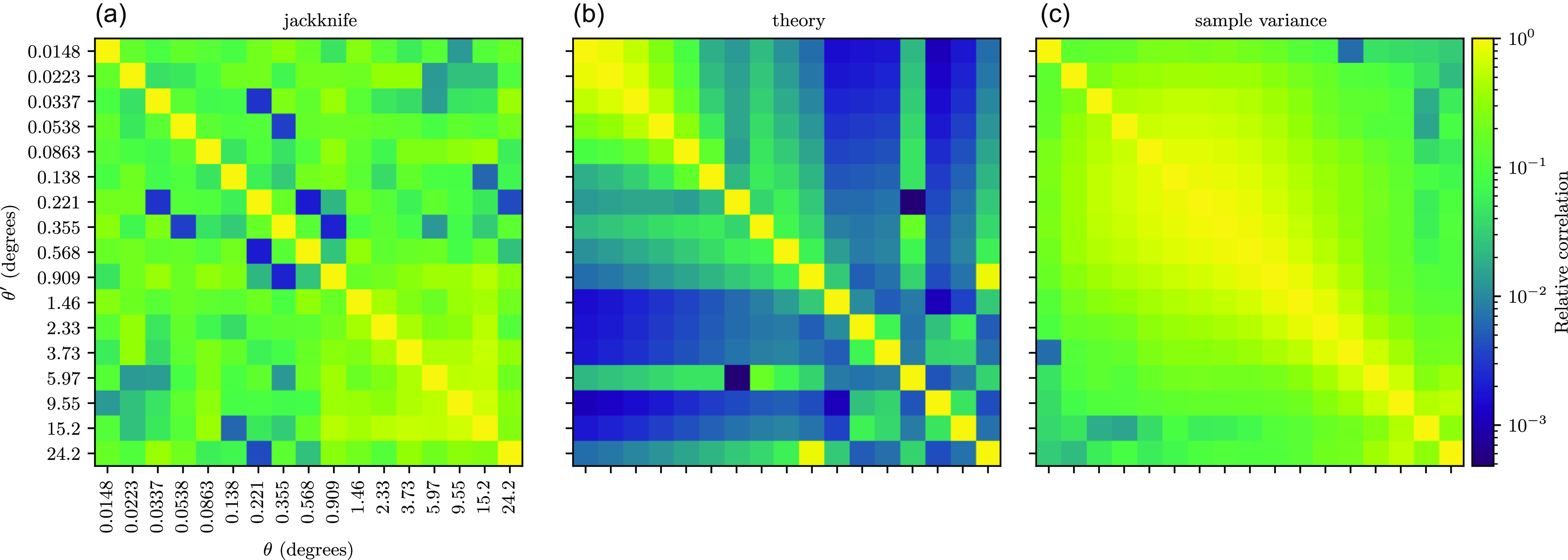
A. Source counts
The tabulated source counts at 200 MHz from the GXDS region, displayed in Fig. 2. The highest flux density counts are incomplete due to small number statistics.
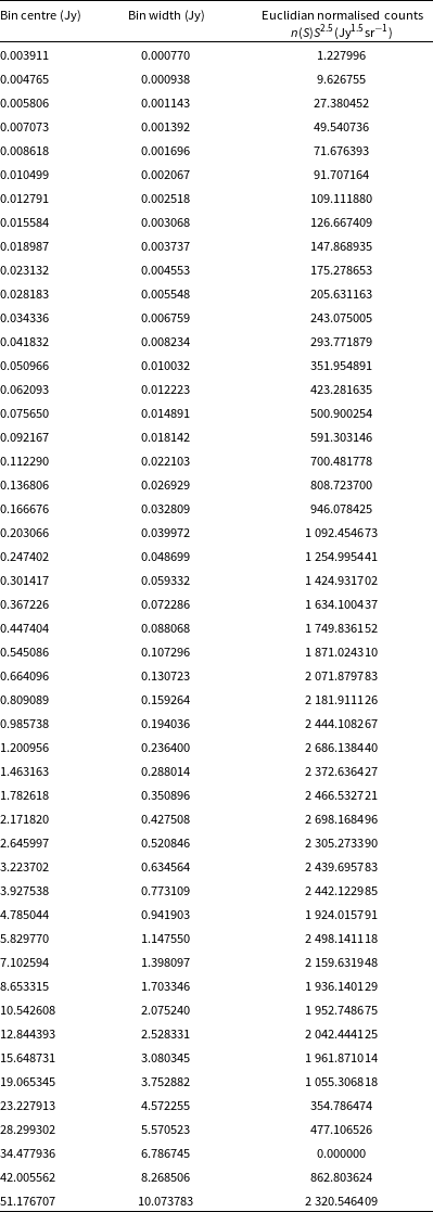
The ACF plotted from each subset of the GXDS region used. The subsets were 20 degrees on a side, with the centre RA and Dec of each listed on the plot.


 Open access