2.1 Radio light curves and sample

The light curves of GRB afterglows display a very different behaviour at radio wavelengths than they do at optical or X-ray wavelengths. At X-ray and optical wavelengths the overall light curve trend is a decaying one, especially after the first hours from the prompt γ-ray emission. The flux usually decays as a power law with time, where its decay rate can vary significantly, both between GRBs and within one GRB light curve. In addition, flares in X-rays and sometimes also in the optical have been found in the first minutes to hours, superimposed on the underlying smooth power-law flux decay.

In the radio bands, however, the light curves are mostly rising during those first hours or days, and peak on a timescale of days to weeks, or even months to years at the lowest radio frequencies. The total duration of the afterglow is also quite different in the radio than at shorter wavelengths. While in X-rays or optical the flux decays typically within several days to weeks below the sensitivity limits of the largest telescopes or satellites, or in the optical it disappears into the host galaxy, some radio afterglows have been detected for months to years. The most famous examples are GRB 970508 (Frail et al. Reference Frail, Kulkarni, Nicastro, Feroci and Taylor1997; Galama et al. Reference Galama1998b; Frail, Waxman, & Kulkarni Reference Frail, Waxman and Kulkarni2000), GRB 980703 (Berger, Kulkarni, & Frail Reference Berger, Kulkarni and Frail2001; Frail et al. Reference Frail2003), and the longest lasting one by far—GRB 030329 (Berger et al. Reference Berger2003a; Frail et al. Reference Frail2005; Resmi et al. Reference Resmi2005; van der Horst et al. Reference van der Horst2005; Pihlström et al. Reference Pihlström, Taylor, Granot and Doeleman2007; van der Horst et al. Reference van der Horst2008; Mesler et al. Reference Mesler, Pihlström, Taylor and Granot2012; Mesler & Pihlström Reference Mesler and Pihlström2013), which is in fact still detectable now, just over a decade after the initial GRB trigger. See the top panels of Figure 1 for the light curves of these three GRBs.

Figure 1.

Radio light curves at 4.9 and 8.5 GHz (top panels) and spectral indices (bottom panels) for GRBs 970508 (Frail et al. Reference Frail, Kulkarni, Nicastro, Feroci and Taylor1997; Galama et al. Reference Galama1998b; Frail et al. Reference Frail, Waxman and Kulkarni2000), 980703 (Berger et al. Reference Berger, Kulkarni and Frail2001; Frail et al. Reference Frail2003), and 030329 (Berger et al. Reference Berger2003a; Frail et al. Reference Frail2005; Resmi et al. Reference Resmi2005; van der Horst et al. Reference van der Horst2005; Pihlström et al. Reference Pihlström, Taylor, Granot and Doeleman2007; van der Horst et al. Reference van der Horst2008; Mesler et al. Reference Mesler, Pihlström, Taylor and Granot2012; Mesler & Pihlström Reference Mesler and Pihlström2013). In contrast with the fast decaying light curves at X-ray and optical frequencies, the radio light curves rise and peak on a time-scale of weeks, and can last for months to years. The spectral index α (where F _ν∝ν^α) between 4.9 and 8.5 GHz varies significantly due to the spectral evolution and scintillation effects. The dashed lines in the bottom panels indicate spectral indices of 2, 1/3, and −0.6 (see Section 2.2 for further details).

The current sample of GRB afterglows with well-monitored radio light curves is small compared to the samples of optical and X-ray light curves. The typical radio fluxes turn out to be relatively close to the detection threshold of the largest radio telescopes, which makes the radio sample sensitivity limited (Chandra & Frail Reference Chandra and Frail2012). However, it has recently been suggested, based on stacking of the radio visibility data of many GRBs, that the low detection rate is due to the presence of two distinct populations of radio-bright and radio-faint GRBs (Hancock et al. Reference Hancock, Gaensler and Murphy2013). However, this analysis cannot determine what the flux distributions of these two tentative populations are. The VLA, with the significantly better sensitivity after its upgrade, and in the future the Square Kilometer Array (SKA), will be able to test whether there is one flux distribution of which we have only seen the tip of the iceberg, or whether there are indeed two distinct populations. If the latter is confirmed, then correlated studies with the properties of afterglows at higher frequencies and the prompt γ-ray emission will provide clues about the nature of this dichotomy: whether they differ in their progenitors or that there is some other fundamental intrinsic difference; or if they differ only in their environments; or that there are some other physical processes affecting the radio detectability.

Even though sensitivity plays an important role in detecting radio afterglows, those that have been detected are not necessarily the nearest ones. The lowest redshift GRBs have been detected at radio frequencies, like GRB 980425 at z = 0.0085 (Kulkarni et al. Reference Kulkarni1998) and GRB 060218 at z = 0.034 (Soderberg et al. Reference Soderberg2006a; Kaneko et al. Reference Kaneko2007); and also the highest redshift ones, GRB 050904 at z = 6.30 (Frail et al. Reference Frail2006) and GRB 090423 at z = 8.26 (Chandra et al. Reference Chandra2010). It has been shown that past z ~ 1 the detection rate is practically insensitive to redshift (Frail et al. Reference Frail2006). Further evidence for this comes from the fact that the samples of radio-detected and non-detected GRBs are from the same redshift populations, and that the average redshift of radio-detected GRBs is z ≃ 1.8, close to the average of the overall sample of GRBs (Chandra & Frail Reference Chandra and Frail2012). This can be explained by the effects of cosmological redshift and time dilation counteracting the dimming due to the source distance (Ciardi & Loeb Reference Ciardi and Loeb2000).

After these general properties of the light curves and sample of GRB radio afterglows, we will now discuss the observational characteristics that provide insight into the physics and dynamics of GRB jets, and put them in context of the existing models.

2.2 Broadband modelling

GRBs are usually modelled and interpreted within the context of the fireball model (Cavallo & Rees Reference Cavallo and Rees1978; Rees & Meszaros Reference Rees and Meszaros1992). However, the jet acceleration mechanism is not very important for its late-time dynamics during the afterglow stage. Compactness arguments imply that the prompt γ-ray emission region must be moving towards us with an ultra-relativistic Lorentz factor, Γ ≳ 10² − 10^2.5 in order to avoid excessive pair production in the source (e.g. Ruderman Reference Ruderman1975; Krolik & Pier Reference Krolik and Pier1991; Lithwick & Sari Reference Lithwick and Sari2001; Granot, Cohen-Tanugi, & do Couto e Silva Reference Granot, Cohen-Tanugi and do Couto e Silva2008). The early onset time of the afterglow emission also suggests that the outflow produced by the central engine is accelerated to ultra-relativistic speeds with bulk Lorentz factors up to several hundreds or more. As the outflow ploughs through the external medium, it sweeps it up by driving a strong relativistic forward external shock into it, while the outflow itself is decelerated by a reverse shock (or by its work on the shocked external medium if the outflow is highly magnetised and thus suppresses the reverse shock). After sweeping up a sufficient amount of external medium the outflow decelerates significantly and transfers most of its energy to the shocked external medium. The forward shock going into the external medium, often referred to as the afterglow shock or blast wave, accelerates swept-up electrons to relativistic random velocities and amplifies the magnetic field behind the shock. As a result, the relativistic electrons emit synchrotron radiation in the magnetic fields behind the shock, thus producing the bulk of the afterglow emission. The synchrotron spectrum is broadband, ranging from radio to X-ray frequencies. Other emission processes like inverse Compton or synchrotron self-Compton radiation may also play a role, but only at X-ray or higher energies and not in the radio regime.

The broadband synchrotron spectrum can be derived by integrating the single-electron spectrum over a power-law distribution of electron energies with slope p (Pacholczyk Reference Pacholczyk1970; Rybicki & Lightman Reference Rybicki and Lightman1979), dN_e /dγ _e ∝ γ^−p _e for γ _e > γ _m . The resulting spectrum can be characterised by the peak flux and usually three characteristic frequencies: the peak frequency ν _m , which corresponds to the minimum energy of the electron energy distribution (γ _e = γ _m ); the cooling frequency ν _c , corresponding to the energetic electrons that cool on the dynamical timescale; and the synchrotron self-absorption frequency ν_sa. These characteristic frequencies are not static but evolve over time, as does the peak flux, resulting in a variety of light curves at different observing frequencies. Figure 2 shows the different possible afterglow synchrotron spectra. Although in principle any ordering of the spectral break frequencies corresponding to any of the five spectra shown in Figure 2 is possible, the most relevant for broadband modelling including radio observations are typically ν_sa < ν _m < ν _c (spectrum 1) for the first days to weeks and ν _m < ν_sa < ν _c (spectrum 2) for later times (Sari et al. Reference Sari, Piran and Narayan1998; Granot & Sari Reference Granot and Sari2002). Note that besides ν_c, ν_m and ν_sa there is a fourth break frequency, ν_ac, which corresponds to the self-absorption frequency of the non-cooled electrons but appears only for fast cooling (ν_c < ν_m, in spectra 4 and 5), which is usually over by the times at which radio afterglows are detected.

Figure 2.

The afterglow synchrotron spectrum, calculated for the Blandford & McKee (Reference Blandford and McKee1976) self-similar solution of an ultra-relativistic spherical blast wave, under standard assumptions, using the accurate form of the synchrotron spectral emissivity and integration over the emission from the whole volume of shocked material behind the forward external (afterglow) shock (for details, see Granot & Sari Reference Granot and Sari2002). The different panels show the five possible broadband spectra of the afterglow synchrotron emission, each corresponding to a different ordering of the spectral break frequencies. Each spectrum consists of several power-law segments (PLSs; each shown with a different colour and labelled by a different letter A–H), which smoothly join at the break frequencies (numbered 1–11). The broken power-law spectrum, which consists of the asymptotic PLSs that abruptly join at the break frequencies (and is widely used in the literature), is shown for comparison. Most PLSs appear in more than one of the five different broadband spectra. Indicated next to the arrows are the temporal scaling of the break frequencies and the flux density at the different PLSs, for a uniform (ISM; k = 0) and stellar wind (WIND; k = 2) external density profile, where ρ_ext = AR ^−k .

The characteristic frequencies and the peak flux can be written in terms of the following macro- and microphysical parameters: the kinetic energy E of the blast wave, the number density n of the surrounding medium (or the mass density ρ_ext = AR ^−k for a power-law external density profile, which is parameterised by A and k), and the ratios ε _B and ε _e , respectively, of the energy density in the magnetic field and in the power-law electron energy distribution, and the total internal energy density (Sari et al. Reference Sari, Piran and Narayan1998; Wijers & Galama Reference Wijers and Galama1999; Granot, Ramirez-Ruiz, & Loeb Reference Granot, Ramirez-Ruiz and Loeb2005). The details of the evolution of the spectrum, and the exact relations between the observable spectral parameters and the derived physical parameters, are determined by the jet dynamics. As an example, Figure 2 shows the temporal scalings of the different break frequencies and fluxes in the different power-law segments of the spectrum, for the Blandford & McKee (Reference Blandford and McKee1976) self-similar solution of a spherical ultra-relativistic blast wave in a uniform or wind-like external medium.

In order to constrain the full set of physical parameters and the jet dynamics, it is essential to obtain well-sampled light curves in the various frequency regimes. While the cooling frequency is typically situated between the optical and X-ray regime or even above the X-ray energy range, ν _m is already below the infrared even at very early times and moves down towards the radio regime, while ν_sa is found at radio frequencies from the first observations onwards. The fact that the peak of the spectrum is below optical and X-ray frequencies causes their light curves to decay from the start, and the radio light curves to rise until the spectral peak passes through the observing bands.

The spectral peak can be ν _m or ν_sa, depending on their ordering at that particular moment (for slow cooling that is most relevant in the radio; see Figure 2), and thus the peak in the radio light curves can correspond to ν _m or ν_sa passing through. This can even vary between light curves at different frequencies for one given GRB, as best illustrated by the light curves of GRB 030329 spanning more than an order of magnitude in observed radio frequencies (Figure 3; van der Horst et al. Reference van der Horst2008). In the bottom right panel of Figure 1 the spectral index between 4.9 and 8.5 GHz evolves from ~2 to ~−0.6 when ν_sa moves through the observing bands, corresponding to spectrum 2 in Figure 2. The spectral index of ~−0.6 is the optically thin one of −(p−1)/2 for p ~ 2.2. The early-time scatter is caused by interstellar scintillation (ISS; Section 2.5.2) while the late-time scatter is due to the low flux levels at late times. The bottom left panel of Figure 1 shows an example of the spectrum 1 in Figure 2. Despite large scatter due to the effects of ISS, it can be seen that for GRB 970508 the spectral index is consistent with 1/3 between ~30 and ~90 d after the burst, after which it evolves to an optically thin spectral index when ν _m evolves to lower frequencies.

Figure 3.

Radio light curves of GRB 030329 (van der Horst et al. Reference van der Horst2008), obtained with WSRT and GMRT (solid symbols), and VLA, ATCA, and Ryle Telescope (open diamonds); open triangles are 3σ upper limits. The dotted line shows a fit to the first 100 d, while the solid line represents a model in which the afterglow shock becomes non-relativistic after 80 d. Both fits are for a homogeneous ambient medium (k = 0). The dash-dotted line represents an alternative model involving a very wide extra jet component suggested by van der Horst et al. (Reference van der Horst2005), which has been disproved by the late-time data at the lowest observing frequencies.

Besides constraining the full broadband spectrum, there is another unique feature of radio light curves in broadband modelling. Since some afterglows are detectable for long times at radio frequencies, the blast wave evolution can be studied once it becomes trans-relativistic and eventually non-relativistic. The non-relativistic phase is of particular interest because it is expected that during the trans-relativistic phase the outflow starts to spread sideways, and eventually approaches spherical symmetry once the blast wave is sufficiently non-relativistic. The latter phase can be used to determine the total energetics without any large uncertainties regarding the jet collimation and relativistic beaming effects, which can influence energy estimates based on broadband modelling at early times. Such radio calorimetry has indeed been done for a few GRBs, most notably GRB 970508 (Frail et al. Reference Frail, Waxman and Kulkarni2000; Berger, Kulkarni, & Frail Reference Berger, Kulkarni and Frail2004), GRB 980703 (Berger et al. Reference Berger, Kulkarni and Frail2004), and GRB 030329 (Frail et al. Reference Frail2005; van der Horst et al. Reference van der Horst2008). For all three GRBs the energy derived by means of this radio calorimetry is a few times 10⁵¹ erg. This is in fact a lower limit to the true energy, both since it is derived through minimum energy considerations, and because of a degeneracy in parameters (Eichler & Waxman Reference Eichler and Waxman2005) where if only a fraction of m_e /m_p < ξ _e ≤ 1 of the electrons takes part in the power-law energy distribution, the observed emission remains unchanged for E→E/ξ _e , ρ→ρ/ξ _e , ε _e →ξ _e ε _e , ε _B →ξ _e ε _B . This arises since the observed emission is determined by the number and energy of the radiating electrons in the power-law energy distribution, the magnetic field strength, and the global dynamics, i.e. the bulk velocity or Lorentz factor and location of the emitting electrons as a function of time, all of which remain unchanged under this transformation of parameter values. Specifically, since E/ρ remains unchanged, then so do all lengths, times, and hydrodynamic dimensionless quantities such as the bulk or random Lorentz factor (see Granot Reference Granot2012). However, the total densities scale as 1/ξ _e , and for each radiating electron in the power-law energy distribution, there are 1/ξ _e protons as well as (1 − ξ _e )/ξ _e non-power-law electrons, which do not contribute to the observed radiation but nonetheless dominate the total energy and cause it to also scales as 1/ξ _e .

2.3 Radio flares and polarisation

Not all GRBs detected in the radio show the characteristic long-term behaviour of radio afterglows. In some GRBs the peak occurs within the first day or couple of days, and the rise and decay can be steeper than the usual decay observed in radio afterglows. This is indicative of a different origin for this early emission, and these radio flares have been attributed to the reverse shock that propagates back into the outflow and decelerates it. This reverse shock emission was first discovered with the bright optical flash (Akerlof et al. Reference Akerlof1999) and following radio flare (Kulkarni et al. Reference Kulkarni1999) in GRB 990123. A second reverse shock candidate came in the same year with GRB 991216 (Frail et al. Reference Frail2000), although the radio light curve decay was in this case less rapid than for GRB 990123. After these two GRBs there have been others with early peaks, but mostly at optical wavelengths and even while prompt γ-rays are still being detected (e.g. Yost et al. Reference Yost2007; Rykoff et al. Reference Rykoff2009), where the most striking example is the naked-eye burst GRB 080319B (Racusin et al. Reference Racusin2008b). These early optical detections, however, are not necessarily of emission coming from the reverse shock, and the majority do not show a radio flare. The few cases that have been suggested to be reverse shock emission are based on only a few observations, which hampers any firm conclusions about the origin of the radio emission.

This situation changed recently with GRB 130427A, a relatively nearby GRB (at z = 0.34), which is very bright across the spectrum, even up to high-energy γ-rays (Perley et al. Reference Perley2013; Ackermann et al. Reference Ackermann2013; Kouveliotou et al. Reference Kouveliotou2013; Preece et al. Reference Preece2013; Maselli et al. Reference Maselli2013). An early optical flash has been reported for this GRB (Vestrand et al. Reference Vestrand2013), and also a very bright radio counterpart has been found within the first day (Laskar et al. Reference Laskar2013; van der Horst et al., in preparation; Anderson et al., in preparation). Broadband modelling from radio to X-ray frequencies at early times requires more than one emission component, and the available data can be well described by a combination of a forward and a reverse shock component (Laskar et al. Reference Laskar2013; Perley et al. Reference Perley2013). The reverse-shock modelling indicates that the jet is moving through a low density medium, a feature that has also been found for GRB 990123. It has been suggested that in these cases the shock cools slowly, which enables the reverse shock to radiate longer than in most other GRBs (Laskar et al. Reference Laskar2013; Perley et al. Reference Perley2013).

An important ingredient for studying GRB jet physics is polarisation, and in particular measuring the polarisation of the reverse shock emission, as it probes the magnetic field structure in the original outflow. Linear polarisation at the few percent level has been found at optical and near-infrared wavelengths when the emission was thought to originate from the forward shock (Covino et al. Reference Covino1999; Wijers et al. Reference Wijers1999; Wiersema et al. Reference Wiersema2012; see, however, Steele et al. Reference Steele, Mundell, Smith, Kobayashi and Guidorzi2009). At radio wavelengths no polarisation has been detected, and the most constraining upper limits for the forward shock polarisation have been determined for GRB 030329 at a level of <1.0% (Taylor et al. Reference Taylor, Momjian, Pihlström, Ghosh and Salter2005) at ν = 8.4 GHz and t = 7.7 d. A contemporaneous optical linear polarisation of 2.2 ± 0.3% was measured (Greiner et al. Reference Greiner2003), but radio polarisation lower than the optical one is likely since ν = 8.4 GHz was below the self-absorption frequency at that time, which suppresses the polarisation. These measurements provide important information regarding the jet, its structure, and the structure of its magnetic field. The magnetic field structure in the original outflow is best constrained by the linear polarisation of the reverse shock emission, and the deepest radio upper limits on it have been obtained for GRB 991216 at less than 7% (Granot & Taylor Reference Granot and Taylor2005). These upper limits seem to indicate that the magnetic field cannot be fully structured on large scales. Although there could be depolarisation due to matter along the line of sight to the GRB, the required large depolarisation is not very likely (Granot & Taylor Reference Granot and Taylor2005).

2.4 Radio prompt emission searches

Radio flares associated with reverse shocks are expected to occur on a timescale of several hours to a few days after a gamma-ray trigger. However, some models predict radio emission at even shorter timescales, in particular models in which the jet is magnetically dominated and coherent radio emission is produced (e.g. Usov & Katz Reference Usov and Katz2000; Sagiv & Waxman Reference Sagiv and Waxman2002; Moortgat & Kuijpers Reference Moortgat and Kuijpers2006). There have been several efforts, before and shortly after the discovery of GRB afterglows, focusing on the detection of such early-time radio emission, especially at low radio frequencies (Baird et al. Reference Baird1975; Inzani et al. Reference Inzani, Sironi, Mandolesi and Morigi1982; Dessenne et al. Reference Dessenne1996; Benz & Paesold Reference Benz and Paesold1998; Balsano Reference Balsano1999). These studies did not result in detections, and the upper limits were not very constraining on any of the models. The GRB locations were at that time also not always as accurately known as they are nowadays, which makes any possible detections of radio bursts and associations with GRBs quite uncertain.

After the discovery of afterglows the focus of radio observations shifted to the longer timescales, but over the last couple of years the prompt radio emission has gained interest at observatories covering both low and high radio frequencies, and using imaging or searches in time series. These observation campaigns have been prompted not only by theoretical considerations, but also by the discovery of fast radio bursts of likely cosmological but unknown origin (Lorimer et al. Reference Lorimer, Bailes, McLaughlin, Narkevic and Crawford2007; Thornton et al. Reference Thornton2013), for which GRBs are possible candidates (Totani Reference Totani2013; Zhang Reference Zhang2013).

The first telescope probing the first minutes to a few hours after GRB triggers in the image plane is AMI, which triggers as soon as possible on any GRB detected by Swift in the Northern Hemisphere (Staley et al. Reference Staley2013). The field of view of AMI is large enough to cover the the Swift/BAT prompt localisation, which makes this kind of immediate follow-up possible. The response times depend on the source position on the sky, but have several times been as fast as 5 min after the GRB trigger. Although for most GRBs this is after the gamma-ray emission has stopped, any prompt radio emission could be delayed, both intrinsically and due to propagation effects in the interstellar and intergalactic medium. The 1 - h observations at 15 GHz result in sensitivities at sub-mJy levels. The earliest detection so far of a GRB radio counterpart was at 8 h after GRB 130427A (Anderson et al., in preparation), which was extremely bright at all energies. At that time the radio emission was produced by the reverse shock (Vestrand et al. Reference Vestrand2013; Laskar et al. Reference Laskar2013; Perley et al. Reference Perley2013) and not by coherent radio emission.

In the time domain a search for short radio flashes was performed with a radio telescope at the Parkes radio observatory, which was triggered on nine GRBs and in which a candidate single pulse at 1.4 GHz was found for two GRBs (Bannister et al. Reference Bannister, Murphy, Gaensler and Reynolds2012). These pulses were 6 and 25 ms long, at 10³ and 5·10² s after the trigger, respectively. Although these two tentative detections are not statistically significant, they are a strong motivation to search for more of these bursts. Several new observatories at low radio frequencies are searching for early-time emission in the image and time domain. The initial results of those studies are starting to surface. For instance, the observations with the first station of the Long Wavelength Array (LWA1), which observes in the tens of MHz range. Odenberger et al. (Reference Odenberger2013) searched through ~18 months of data in the LWA1 archive at the trigger times, and following few hours (to account for the propagation delays in the interstellar and intergalactic medium), of GRBs detected by Swift/BAT, the Monitor of All-sky X-ray Image (MAXI) aboard the International Space Station, and the Fermi Gamma-ray Burst Monitor (GBM). Although the positional accuracy of the latter is typically several degrees, the field-of-view of LWA1 at its low observing frequencies is large enough to cover a significantly large fraction of the sky than the Fermi/GBM location uncertainty region. No prompt GRB emission has been found in images with 5 s integration times, at sensitivities better than previous studies, but these sensitivities are still far from what will be reached by several new low-frequency radio telescopes in the near future (see Section 6.1).

2.5 Size measurements

For several types of sources, it is possible to make images of the jet. Using ‘regular’ imaging is possible for the large-scale AGN jets, but very long baseline interferometry (VLBI) is required for the smallest scales in AGN jets or for the jets in X-ray binaries. Directly imaging the jet, or measuring the size of the jet and its evolution, are important for constructing and testing the theoretical models. Since GRBs are found at cosmological distances but their jets are smaller than a parsec in size, obtaining resolved images is extremely hard even with VLBI. Nonetheless, the image size evolution has been measured in one relatively nearby case, GRB 030329. The source size evolution can also be determined indirectly by utilising the effects of ISS, as has been done for a few GRBs. In this section, we discuss the results of these direct and indirect size measurements, and their implications for broadband modelling.

2.5.1 Very Long Baseline Interferometry

GRB 030329 was bright at all observable frequencies, mainly due to its low redshift of z = 0.1685. Its proximity and radio brightness made a direct size measurement using VLBI possible for the first and only time thus far. Global VLBI was necessary to reach sub-milliarcsecond (mas) resolution: at 25 d the source was 0.07 mas in sizeFootnote ¹ and it was 0.17 mas at 83 d (Taylor et al. Reference Taylor, Frail, Berger and Kulkarni2004). Given the redshift, this implies source sizes of 0.2 and 0.5 parsec, respectively, and an average apparent expansion speed between the two epochs of 3 − 5 times the speed of light (and a slightly higher value between the time of the GRB and the first epoch; see Figure 4).

Figure 4.

Evolution of the source size of GRB 030329. All the solid symbols are size measurements or upper limits obtained with VLBI (Taylor et al. Reference Taylor, Frail, Berger and Kulkarni2004; Reference Taylor, Momjian, Pihlström, Ghosh and Salter2005; Pihlström et al. Reference Pihlström, Taylor, Granot and Doeleman2007; Mesler et al. Reference Mesler, Pihlström, Taylor and Granot2012), while the open symbol indicates an estimate based on scintillation effects (Berger et al. Reference Berger2003a). Top panel: evolution of the angular diameter (in milli-arcseconds; left y-axis) and the corresponding physical size D (in cm; right y-axis). Bottom panel: evolution of the average apparent expansion velocity ⟨β_app⟩ = (1 + z)D/2ct. Note that 1 mas corresponds to 2.85 pc at the redshift z = 0.1685 of GRB 030329.

This was a direct proof of the relativistic expansion of GRB jets and provided support for the fireball model (Oren, Nakar, & Piran Reference Oren, Nakar and Piran2004; Granot et al. Reference Granot, Ramirez-Ruiz and Loeb2005a), since the measured image size agreed with the expectations from afterglow models, which only weakly depends on the model parameters (although it does not tell us anything about the outflow composition or jet acceleration mechanism). After the first VLBI observations there have been two more source size measurements, at 217 d (Taylor et al. Reference Taylor, Momjian, Pihlström, Ghosh and Salter2005) and 806 d (Pihlström et al. Reference Pihlström, Taylor, Granot and Doeleman2007), and a constraining upper limit at 2032 d, i.e. ~5.5 yr after the GRB trigger (Mesler et al. Reference Mesler, Pihlström, Taylor and Granot2012). The source size measurements have been combined with broadband modelling of the available radio light curves to better constrain the physical parameters and possibly the lateral spreading of the jet (Granot et al. Reference Granot, Ramirez-Ruiz and Loeb2005a; Pihlström et al. Reference Pihlström, Taylor, Granot and Doeleman2007; Mesler et al. Reference Mesler, Pihlström, Taylor and Granot2012; Mesler & Pihlström Reference Mesler and Pihlström2013). Although the latter could not be significantly constrained, modelling of the light curves and source size evolution gave consistent results, for instance in the derived physical parameters like the blast wave energy and the transition from the trans-relativistic to non-relativistic expansion phase.

Besides the size measurements, constraints on the proper motion have also been placed by the VLBI observations: <0.07 mas/yr using the latest VLBI observation, implying an upper limit <0.73 c (Mesler et al. Reference Mesler, Pihlström, Taylor and Granot2012). This upper limit is consistent with the picture that in order to see the prompt γ-ray emission our line of sight should be within the initial jet aperture, in which case the cumulative proper motion of the flux centroid is indeed expected to be less than the current radius (i.e. half the diameter) of the image (Granot & Loeb Reference Granot and Loeb2003; Pihlström et al. Reference Pihlström, Taylor, Granot and Doeleman2007; Mesler et al. Reference Mesler, Pihlström, Taylor and Granot2012), or equivalently, the mean proper motion speed is less than the average apparent expansion velocity of the image (shown in the lower panel of Figure 4). This is in contrast with viewing the jet significantly off of its symmetry axis, in which case the cumulative proper motion could exceed the image size (Granot & Loeb Reference Granot and Loeb2003). One more implication is that the cannonball model, in which plasmoids with extremely high Lorentz factors are ejected instead of a jet (Dado, Dar, & De Rujula Reference Dado, Dar and De Rujula2004), is inconsistent with the proper motion upper limits (Mesler et al. Reference Mesler, Pihlström, Taylor and Granot2012).

2.5.2 Interstellar scintillation

Variations in the observed radio flux due to ISS have been observed in many sources, mainly pulsars and AGN. There are different types of scintillation, depending on the observing frequency and the angular size of the object. In general, propagation effects in the interstellar medium cause the flux of a compact source to vary, while a source larger than a certain angular size will not display this behaviour (Rickett Reference Rickett1990). GRBs have shown strong modulations of their radio light curves (Goodman Reference Goodman1997), with the first example being GRB 970508 (Frail et al. Reference Frail, Kulkarni, Nicastro, Feroci and Taylor1997; Reference Frail, Waxman and Kulkarni2000), and many more GRBs since then having displayed a similar behaviour. These variations do not only occur between observations on different days, but also intra-day variability has been observed, for instance in GRB 070125 (Chandra et al. Reference Chandra2008). In all GRBs the variations become weaker over time, because of the jet's evolution: its angular size starts out smaller than the characteristic angular scale for ISS, but it grows with time until it eventually exceeds this scale and the variations become smaller. Measuring the strength of this scintillation behaviour and the time at which it quenches provide an indirect estimate of the source size.

There are in general two types of ISS: weak and strong scattering. In weak scattering there are only small phase changes over the first Fresnel zone of the radio waves due to fluctuations in the density of free electrons in the medium in between us and the source, usually in the interstellar medium of our galaxy. When the wavefront is highly distorted on scales smaller than the first Fresnel zone, this is called strong scattering and produces much larger flux modulations than weak scattering. Strong scattering can be divided up into: (i) refractive scintillation, caused by focusing and defocusing of the wave front by large-scale inhomogeneities, which is a broadband phenomenon; and (ii) diffractive scintillation, caused by interference between rays diffracted by small-scale irregularities in the interstellar medium, which is modulating the flux over a narrow frequency band.

For any particular GRB the angular scales for the three types of ISS, as well as the scintillation strength and timescale, can be estimated (Walker Reference Walker1998) using the NE2001 model of the distribution of free electrons in our galaxy (Cordes & Lazio Reference Cordes and Lazio2002). The scintillation strength is first of all determined by the observing frequency. Observations above a transition frequency ν₀ are typically in the weak scattering regime, while observations at lower frequencies are affected by strong scattering. The angular scales and modulation indices, i.e. the fractional flux variations (or the ratio of the standard deviation and mean value of the flux density), can be expressed in terms of the angular size of the first Fresnel zone θ_F0 at an observing frequency ν equal to the transition frequency ν₀, with θ_F0 = 2.1 × 10⁴ SM ^0.6ν ^{− 2.2} ₀μas. The scattering measure SM and ν₀ depend on the location of the source in the sky and can be determined from the NE2001 model (Cordes & Lazio Reference Cordes and Lazio2002), with typical values of SM ~ 10^−3.5 kpc/m^20/3 and ν₀ ~ 10 GHz, resulting in values for θ_F0 of a few μas. The equations for the angular scale, time scale and modulation index, for weak, refractive and diffractive scintillation are given in Table 1. It is clear from this table that the modulation indices for weak and refractive scattering are highest when the observing frequency is close to ν₀, but they are always smaller than the modulation index of diffractive scattering, which is 1 for the source angular size θ_s < θ_d. The angular size for diffractive scintillation is smaller than for refractive or weak scattering though, so for GRB radio afterglows it can only play a significant role at early times when the jet is still compact enough. Furthermore, diffractive scintillation is a narrow-band phenomenon, and is only a significant effect when one observes with a frequency resolution Δν_obs < Δν_dc = ν(ν/ν₀)^17/5, while for Δν_obs>Δν_dc the modulation index will be suppressed by a factor of ~N ^−1/2 = (Δν_obs/ν)^−1/2(ν/ν₀)^17/10 due to effective averaging over N = Δν_obs/Δν_dc mutually incoherent frequency ranges, each with the decorrelation bandwidth Δν_dc.

Table 1.

Angular scales, time scales, and modulation indices for weak, refractive, and diffractive ISS, with ν₀ the transition frequency between weak and strong scattering, θ_F0 the angular size of the first Fresnel zone at this frequency, ν the observing frequency, and θ_s the source angular size. For GRBs, ν₀ is typically ~10 GHz and θ_F0 is a few μas.

Figure 1 shows the effects of scintillation on three well-studied GRBs. GRB 030329 was relatively nearby, and as a result ISS affected the light curves only in the first couple of weeks, since the source size became larger than the ISS angular sizes quickly. The angular size at which this happened could be estimated, as shown in Figure 4. GRBs 970508 and 980703 were situated at a higher redshift, and thus the ISS effects lasted longer. Quenching of the scintillation could also be used in those two GRBs to estimate the source size evolution, which was consistent with the results from broadband modelling (Frail et al. Reference Frail, Waxman and Kulkarni2000). We note that the NE2001 model provides rather good estimates for lines-of-sight in our galaxy, but is quite uncertain for sources off the galactic plane. Therefore the size estimates for GRBs based on this method should be treated with caution. Some broadband modelling efforts include scintillation estimates by adding them to the radio flux uncertainties, to account for the large values of their fitting statistic (usually χ²), but this should be done cautiously.

2.6 Searching for off-axis GRB jets

So far we have discussed the observations of GRB afterglows for which we have detected the prompt γ-ray emission. Given the collimation of GRB outflows, combined with relativistic beaming effects, there is also a large fraction of the total population of GRBs for which we do not see any emission coming from the jet at early times, and in particular we do not detect their prompt γ-ray emission. However, the deceleration of the jet during the afterglow and its eventual sideways expansion cause the beaming of its radiation to decrease with time. Eventually, at sufficiently late times, the expanding beaming cone of the afterglow radiation reaches our line of sight and the jet's afterglow emission becomes visible. The importance of such events for constraining the degree of collimation of GRB jets was realised early on (Rhoads Reference Rhoads1997), and they have been called ‘orphan afterglows’. No orphan afterglow has been clearly detected yet, but their detection prospects and implications of existing limits on the detection rate have been studied at X-ray (Woods & Loeb Reference Woods and Loeb1999; Nakar & Piran Reference Nakar and Piran2003), optical (Dalal, Griest, & Pruet Reference Dalal, Griest and Pruet2002; Totani & Panaitescu Reference Totani and Panaitescu2002; Nakar, Piran, & Granot Reference Nakar, Piran and Granot2002; Rhoads Reference Rhoads2003; Rau, Greiner & Schwartz Reference Rau, Greiner and Schwartz2006) and radio (Perna & Loeb Reference Perna and Loeb1998; Levinson et al. Reference Levinson, Ofek, Waxman and Gal-Yam2002; Gal-Yam et al. Reference Gal-Yam2006; Soderberg et al. Reference Soderberg, Nakar, Berger and Kulkarni2006b; Bietenholz et al. Reference Bietenholz, De Colle, Granot, Bartel and Soderberg2013) frequencies.

Eventually, the emission from the jet becomes roughly isotropic, varying only by a factor of order unity between different observers, when the jet becomes sub-relativistic, as well as more spherical, on a time scale of months to years after the GRB. At such late times the afterglow is detectable only at radio frequencies. Since GRBs of the long-soft class—a large fraction of all GRBs—are associated with Type Ic SNe, it has been suggested to search for such orphan radio afterglows at late times at the positions of relatively nearby SNe of this type (Paczynski Reference Paczynski2001; Granot & Loeb Reference Granot and Loeb2003), and there have been searches dedicated to this purpose (e.g. Berger et al. Reference Berger, Kulkarni, Frail and Soderberg2003b; Soderberg et al. Reference Soderberg, Nakar, Berger and Kulkarni2006b; Bietenholz et al. Reference Bietenholz, De Colle, Granot, Bartel and Soderberg2013). These searches have not resulted in any clear detections of off-axis GRB jets so far.

There have been Type Ic SNe detected at radio wavelengths that were considered as off-axis jet candidates, such as SN 2001em (Granot & Ramirez-Ruiz Reference Granot and Ramirez-Ruiz2004). Given its proximity, with a distance of ~80 Mpc, an initially relativistic jet would have been resolved with VLBI, but the observations showed an unresolved source (Bietenholz & Bartel Reference Bietenholz and Bartel2005; Paragi et al. Reference Paragi2005; Bietenholz & Bartel Reference Bietenholz and Bartel2007; Schinzel et al. Reference Schinzel, Taylor, Stockdale, Granot and Ramirez-Ruiz2009). This has lead to the suggestion that the radio emission was produced by an interaction of the SN ejecta with a dense circumstellar shell (Chugai & Chevalier Reference Chugai and Chevalier2006). We note that there have been other SNe that were detected at radio frequencies within a few days after the optical discoveries and were candidates for jet-like emission. SN 2008D was discovered because of an X-ray flash, but modelling of the radio light curves and VLBI observations led to the conclusion that the emitting outflow was non-relativistic (Soderberg et al. Reference Soderberg2008; Bietenholz, Soderberg, & Bartel Reference Bietenholz, Soderberg and Bartel2009; van der Horst et al. Reference van der Horst2011). SN 2009bb was extremely radio bright, and based on the light curves, Soderberg et al. (Reference Soderberg2010) concluded that the ejecta were mildly relativistic (~0.85c), which could not be further constrained with VLBI observations (Bietenholz et al. Reference Bietenholz2010). While the latter velocity determination was model dependent, for SN 2007gr (Paragi et al. Reference Paragi2010) the size expansion was constrained directly with VLBI to be mildly relativistic (at least ~0.6c). However, in the latter case Soderberg et al. (Reference Soderberg, Brunthaler, Nakar, Chevalier and Bietenholz2010) concluded from modelling of the radio and X-ray light curves that the expansion is non-relativistic (~0.2c). For a more detailed review of the VLBI results on Type Ic SNe including the off-axis jet candidates, see Bietenholz (Reference Bietenholz2013).

Despite a number of interesting candidates for mildly relativistic and/or collimated outflows from radio SNe, there have been no clear detections of off-axis relativistic GRB-like jets to this date. In principle this could put constraints on the number of Type Ic SNe harbouring jets, or on the average jet opening angle. However, it should be noted that the SNe associated with GRBs have broad lines in their optical spectra, which significantly reduces the sample of candidates for off-axis GRB jet emission. Nevertheless, current limits imply that only a fraction of such broad-lined SNe Ib/c could harbour energetic, relativistic jets that produce bright radio emission, with luminosities comparable to observed radio afterglows of GRBs at cosmological distances (Bietenholz et al. Reference Bietenholz, De Colle, Granot, Bartel and Soderberg2013). Moreover, radio surveys of nearby SNe Ib/c are also useful for constraining the presence of other types of relativistic jets that do not reach high enough Lorentz factors to produce a GRB and/or are somewhat less energetic (Granot & Ramirez-Ruiz Reference Granot and Ramirez-Ruiz2004). This arises since as long as the jet initially reaches a Lorentz factor Γ₀≳ a few, its late-time radio emission (after its deceleration radius) is largely independent of Γ₀. The latter also holds at earlier times, around or after the peak time, for off-axis viewing angles that are outside of the jet's initial beaming cone, i.e. as long as Γ₀ > 1/(θ_obs − θ₀). This can be very interesting for constraining the fraction of engine-driven SNe Ib/c, which may also be related to the large typical inferred asphericity of these explosions.

3.1 The jet angular structure

Most works consider a jet with axial symmetry, both for simplicity, and since this is expected to zeroth order in most theoretical models. Moreover, the jet is usually assumed to be double-sided, with reflection symmetry about the plane normal to its symmetry axis that intersects the central source. The angular structure of such a jet can be described by the dependence on polar angle θ (in the range 0 ≤ θ ≤ π/2) of the initial distribution of its total energy (excluding rest energy) content per solid angle, $\mathcal {E}$ , and its initial Lorentz factor Γ₀. The initial Lorentz factor distribution, Γ₀(θ), affects mainly the prompt γ-ray emission and early afterglow, as it is largely forgotten after the local deceleration time or radius t _dec(θ) ~ R _dec(θ)/2cΓ² ₀(θ), while $\mathcal {E}(\theta )$ affects also the late-time afterglow emission. The structure of GRB jets is important for deducing their event rate and total energy, as well as for requirements on the jet production mechanisms. Several different jet structures have been suggested in the literature. They are shown in Figure 5 and briefly discussed below.

Figure 5.

An illustration of various jet structures that have been discussed in the literature, in terms of the initial distribution of their energy per solid angle (excluding rest energy), $\mathcal {E} = dE/d\Omega$ , with the angle θ from the jet symmetry axis, in a log-log scale. Both the normalisation of $\mathcal {E}$ and the typical angular scale may vary in most models, and their values in this figure were chosen to be more or less typical (from Granot Reference Granot2005).

The uniform jet (UJ, or ‘top hat’) model is the most popular model for the angular structure of GRB jets (Rhoads Reference Rhoads1997; Reference Rhoads1999; Panaitescu & Mészáros Reference Panaitescu and Mészáros1999; Sari et al. Reference Sari, Piran and Halpern1999; Kumar & Panaitescu Reference Kumar and Panaitescu2000a; Moderski, Sikora, & Bulik Reference Moderski, Sikora and Bulik2000; Granot et al. Reference Granot, Miller, Piran, Suen, Hughes, Costa, Frontera and Hjorth2001; Reference Granot, Panaitescu, Kumar and Woosley2002; Ramirez-Ruiz & Madau Reference Ramirez-Ruiz and Madau2004; Ramirez-Ruiz et al. Reference Ramirez-Ruiz, Granot, Kouveliotou, Woosley, Patel and Mazzali2005), where $\mathcal {E}$ and Γ₀ are uniform within some finite half-opening angle, θ_j, and sharply drop outside of θ_j (thick solid blue line in Figure 5). Another rather popular jet structure is the universal structured jet (USJ) model (Mészáros, Rees, & Wijers Reference Mészáros, Rees and Wijers1998; Lipunov, Postnov, & Prokhorov Reference Lipunov, Postnov and Prokhorov2001; Rossi, Lazzati, & Rees Reference Rossi, Lazzati and Rees2002; Zhang & Mészáros Reference Zhang and Mészáros2002), where $\mathcal {E}$ and Γ₀ vary smoothly with θ, as a power law outside of some narrow core angle, usually with equal energy per decade in θ, $\mathcal {E}\propto \theta ^{-2}$ (thick dashed red line in Figure 5). The power-law wings can either extend all the way to the equator (θ = π/2), or terminate at a somewhat smaller angle, but still of order unity, as the universality requires it to accommodate the largest inferred angles of tens of degrees. In the UJ model the different values of the jet break time, t _j, in the afterglow light curve arise mainly due to different initial values θ₀ for θ_j (and to a lesser degree due to different ambient densities). In the USJ model, all GRB jets are assumed to be identical, and the different values of t _j arise mainly due to different viewing angles, θ_obs, from the jet axis. Moreover, the expression for t _j is similar to that for a uniform jet with $\mathcal {E}\rightarrow \mathcal {E}(\theta =\theta _{\rm obs})$ and θ₀→θ_obs.

An alternative jet structure with a Gaussian angular profile (thin dashed-dotted green line in Figure 5) has also been proposed in the literature (Zhang & Mészáros Reference Zhang and Mészáros2002; Kumar & Granot Reference Kumar and Granot2003). The main reasoning behind it is that it can serve as a more realistic version of a uniform jet, where the edges are smooth rather than sharp. A Gaussian jet, $\mathcal {E}(\theta )\propto \exp (-\theta ^2/2\theta _0^2)$ , can be thought of as being intermediate between the UJ and USJ models. It is, however, closer to the UJ model than to the canonical version of USJ model, which has equal energy per decade in the wings ( $\mathcal {E}\propto \theta ^{-2}$ , where the wings dominate the total jet energy by about an order of magnitude) in the sense that the energy in the wings of a Gaussian jet is much smaller than in its core.

An additional jet structure that is gradually being considered more seriously is a two-component jet (Pedersen et al. Reference Pedersen1998; Frail et al. Reference Frail2000; Berger et al. Reference Berger2003a; Huang et al. Reference Huang, Wu, Dai, Ma and Lu2004; Peng, Königl, & Granot Reference Peng, Königl and Granot2005; Racusin et al. Reference Racusin2008a), with a narrow uniform jet of initial Lorentz factor Γ₀ ≳ 100 surrounded by a wider uniform jet with Γ₀ ~ 10 − 30 (thin dashed black line in Figure 5). A jet structure with such properties was predicted both in the context of the cocoon in the collapsar model (Ramirez-Ruiz, Celotti, & Rees Reference Ramirez-Ruiz, Celotti and Rees2002) and in the context of a hydromagnetically driven neutron-rich jet (Vlahakis, Peng, & Königl Reference Vlahakis, Peng and Königl2003). Phenomenologically, this model was invoked to explain rebrightening episodes in the afterglow light curves of GRBs 030329 (Berger et al. Reference Berger2003a) and 030723 (Huang et al. Reference Huang, Wu, Dai, Ma and Lu2004). Detailed calculations, however, show that it cannot produce very sharp features in the light curve (Granot Reference Granot2005), and in particular cannot account for these sharp observed rebrightening episodes. Another motivation for such a jet structure arises from the energetics of GRBs, as it might help reduce the high efficiency requirements from the prompt γ-ray emission (Peng, Königl, & Granot Reference Granot2005). Later Swift observations (e.g. Nousek et al. Reference Nousek2006) have taught us, however, that the two-component jet model does not significantly help reduce the required γ-ray efficiency (Granot, Königl, & Piran Reference Granot, Königl and Piran2006) despite being able to reproduce the early X-ray afterglow light curves.

Another jet structure that has been suggested (Levinson & Eichler Reference Levinson and Eichler1993; Reference Levinson and Eichler2000; Eichler & Levinson Reference Eichler and Levinson2003; Reference Eichler and Levinson2004; Lazzati & Begelman Reference Lazzati and Begelman2005; Tchekhovskoy, McKinney, & Narayan Reference Tchekhovskoy, McKinney and Narayan2008) has a cross-section in the shape of a ring at angle θ _c , and is sometimes referred to as a ‘hollow cone’ (thin solid magenta line in Figure 5), which is uniform within θ _c < θ < θ _c +Δθ where Δθ ≪ θ _c . An extreme variant of this structure is a ‘fan’ shaped jet where Δθ ≪ θ _c +Δθ = π/2 (thick dashed-dotted cyan line in Figure 5). However, it produces only a modest steepening across the jet break (Granot Reference Granot2005) and is not very well motivated on theoretical grounds.

Finally, there are non-axi-symmetric jet structures that have been suggested in the literature, such as the ‘patchy shell’ model (Kumar & Piran Reference Kumar and Piran2000; Nakar & Oren Reference Nakar and Oren2004) or its extreme version—the ‘mini-jets’ model (Yamazaki, Ioka, & Nakamura Reference Yamazaki, Ioka and Nakamura2004). For a more detailed discussion of the different models for the jet angular structure and how they might be constrained using GRB observations we refer readers to Granot (Reference Granot2007) or Granot & Ramirez-Ruiz (Reference Granot, Ramirez-Ruiz, Kouveliotou, Woosley and Wijers2013). For the purposes of this review it is most important to mention that the jet angular structure might be probed using afterglow observations, and in particular the shape of the afterglow light curves and the evolution of its linear polarisation.

From all the topics on jet dynamics that are discussed in the next section, the one that is most strongly affected by the jet's initial angular structure is its late-time dynamics well after the energy in the outflow is transferred to the shocked external medium. There we will consider primarily a UJ model, since it has been most extensively studied.

3.2 Light curves for different observers

Examples of afterglow light curves for different jet models and viewing angles are shown in Figure 6 for the optical and in Figure 7 in the radio. For an initially perfectly uniform jet with sharp edges, numerical simulations show that slower material is generated at the sides of the jet, whose velocity points sideways relative to the spherical radial direction. Both effects cause less beaming of the radiation within the jet aperture leading to more flux seen by observers at large off-axis viewing angles (θ_obs>θ₀), and a more gradual rise to the peak, with a peak flux that is larger compared to that for an on-axis observer at the same observed time. This can be seen when comparing the top and second panel of Figures 6 and 7. For large off-axis viewing angles the peak occurs when the beaming cone of the jet's radiation reaches our line of sight, and then the light curve approaches that for an on-axis observer. In the top panel of Figure 7 the hydrodynamic simulation has been supplemented before its onset with a conical wedge with half-opening angle θ₀ = 0.2 taken out of the Blandford & McKee (Reference Blandford and McKee1976) self-similar solution that was also used for its initial conditions. The transition between the two can be seen as a sharp increase in flux that quickly saturates to a shallower rise of the flux. Before this transition the flux rises rapidly, similar to the semi-analytic models, while after the transition it rises more moderately because of the hydrodynamics effects mentioned above. It is important to keep such effects in mind when using a simple (semi-)analytic jet model.

Figure 6.

Afterglow optical (ν = 5 × 10¹⁴ Hz) light curves for different jet angular structures, dynamics, and viewing angles (from Eichler & Granot Reference Eichler and Granot2006). The viewing angles are θ_obs/θ₀ = 0, 0.5, 1, 1.5, 2, 3, 4, 5, where θ₀ is the (initial) half-opening angle for the uniform jet (two top panels) and the core angle (θ₀ = 0.1) for the Gaussian jet (two bottom panels). Top panel: an initially uniform jet with sharp edges and half-opening angle θ₀ = 0.2 whose dynamics are calculated using a hydrodynamic simulation (Granot et al. Reference Granot, Panaitescu, Kumar and Woosley2002). The other panels show results for a semi-analytic dynamical model (without lateral spreading). Second panel: a uniform jet with sharp edges (θ₀ = 0.1). Two bottom panels: a Gaussian jet, in energy per solid angle $\mathcal {E}$ , and either a Gaussian or uniform initial Lorentz factor Γ₀. All cases do not include a counter-jet, and thus the light curves are not shown up to very late times.

Figure 7.

Similar to Figure 6 but in the radio (ν = 1 GHz). The hydrodynamic simulations (top panel) are from J. Granot, F. De Colle, & E. Ramirez-Ruiz, in preperation, as in Figure 8, and include a counter-jet that produces a late-time bump in the light curves. For the semi-analytic models, shown in the bottom three panels, there is no lateral spreading and no counter-jet (which makes them not very realistic at late times). In all cases E _k,iso = 10⁵³ erg, n = 1 cm⁻³, p = 2.5, ε _e = ε _B = 0.1. The sharp break in the on-axis (θ_obs = 0) light curve corresponds to the passage of ν _m (from ν < ν _m < ν _c before the break to ν _m < ν < ν _c after the break; self-absorption is not included here). The jet break is earlier and is much less pronounced in the radio, and thus much harder to observe.

For a jet with a Gaussian distribution of $\mathcal {E}(\theta )$ , if Γ₀(θ) also has a Gaussian profile (which corresponds to a constant rest mass per solid angle in the outflow), then the afterglow light curves are rather similar to those for a uniform jet (third panel of Figures 6 and 7; Kumar & Granot Reference Kumar and Granot2003). On the other hand, for a Gaussian $\mathcal {E}(\theta )$ but a constant Γ₀(θ) the light curves for off-axis viewing angles (i.e. outside the jet's core) have a much higher flux at early times, compared to a Gaussian Γ₀(θ) or a uniform jet because of a dominant contribution from the jet material that emits along the line of sight, which in this case has an early deceleration time (bottom panel of Figures 6 and 7; Eichler & Granot Reference Eichler and Granot2006; Granot, Ramirez-Ruiz, & Perna Reference Granot, Ramirez-Ruiz and Perna2005). After this material along the line of sight is decelerated by the external medium, the light curves join those for an initially Gaussian Γ₀(θ) (compare the third and bottom panels of Figures 6 and 7).

Figure 8 shows light curves based on hydrodynamic simulations (De Colle et al. Reference De Colle, Granot, Lopez-Camara and Ramirez-Ruiz2012a; Reference De Colle, Ramirez-Ruiz, Granot and Lopez-Camara2012b), for different viewing angles and a power-law external density profile (ρ_ext = AR ^−k ) ranging from a uniform medium as expected for the ISM (k = 0) to a wind-like profile (k = 2 for a constant mass-loss stellar wind). It also includes two intermediate cases (k = 1, 1.5), which might correspond to the wind of a massive star progenitor whose properties vary near the end of its life. The late-time bump in the light curve corresponding to the counter-jet coming into view is clearly present for a k = 0 but becomes less pronounced as k increases and almost disappears for k = 2 (De Colle et al. Reference De Colle, Ramirez-Ruiz, Granot and Lopez-Camara2012b). The rise to the peak for large off-axis viewing angles is also much less sharp for larger k (more stratified external media compared to a uniform medium with k = 0) as the jet decelerates more slowly causing its beaming cone to approach the line of sight more gradually.

Figure 8.

Afterglow radio (ν = 1 GHz) light curves for hydrodynamic simulations of an initially uniform jet for different viewing angles, θ_obs = 0, 0.4, 0.8, π/2, and different values of the external density power-law index, k = 0, 1, 1.5, 2, where ρ_ext = AR ^−k (from J. Granot et al., in preparation). Initial conditions are a conical wedge of half-opening angle θ₀ = 0.2 rad taken out of the Blandford & McKee (Reference Blandford and McKee1976) self-similar spherical solution with an energy of E _k,iso = 10⁵³ erg (and a true energy E≈2 × 10⁵¹ erg for a double-sided jet) when the Lorentz factor of matter just behind the shock is 20. The external density is chosen to be n ₀ = 1 cm⁻³ for k = 0 and to have the same jet-break radius (and approximately the same density at that radius) for k>0 (corresponding to A _* = 1.65 for k = 2). The light curves are supplemented by the emission from before the simulation onset time using a conical wedge like that used in the initial conditions.

4.1 Magnetic acceleration

Magnetic acceleration likely plays a key role not only in GRBs, but also in other relativistic jet sources, such as AGN or micro-quasars. It has been realised early on that the (quasi-steady) thermal acceleration (the main competing acceleration mechanism) and collimation of initially very hot and high-pressure material near the source to highly super-sonic speeds (e.g. the ‘twin exhaust’ model for AGN jets; Blandford & Rees Reference Blandford and Rees1974) faces serious difficulties under realistic astrophysical conditions (i.e. it is subject to various instabilities; Smith et al. Reference Smith, Norman, Wilson and Smarr1981). Therefore, in light of the difficulties faced by thermal acceleration, magnetic fields play an important role in many models for the launching, collimation and acceleration of relativistic jets. In particular, in AGN jets the Thompson optical depth even near the source is not high enough for thermal acceleration by the radiation pressure to work well.

Most magnetic acceleration models assume a steady flow, as this may adequately describe outflows that vary slowly enough with time, and since it significantly simplifies the relevant dynamical equations, allowing analytic self-similar solutions (e.g. Begelman & Li Reference Begelman and Li1992; Vlahakis & Königl Reference Vlahakis and Königl2003) with the additional standard assumptions of axial symmetry and ideal MHD (i.e. no dissipation of magnetic energy). An advantage of magnetic acceleration is that strong large-scale magnetic fields near the source may help avoid excessive mass loading and thus enable the jets to reach relativistic speeds.

It has been known for a long time (Goldreich & Julian Reference Goldreich and Julian1970) that a (quasi-)spherical highly magnetised steady flow can effectively accelerate only up to an asymptotic Lorentz factor Γ_∞ ~ σ^1/3 ₀ and magnetisation σ_∞ ~ σ^2/3 ₀ where σ₀ ≫ 1 is the initial value of the magnetisation parameter σ (the ratio of electromagnetic to matter energy flux or enthalpy density). That is to say, most of the energy remains in electromagnetic form, i.e. a Poynting flux dominated flow. Collimation of the flow by an external pressure that leads to an asymptotic jet half-opening angle θ_j can increase Γ_∞ and decrease σ_∞ by up to a factor of ~θ^−2/3 _j. This occurs since lateral causal contact in the jet (that is required for efficient acceleration) is maintained if θ_j does not exceed the Mach angle, θ_j ≲ θ_M ~ σ^1/2/Γ, where energy conservation implies σΓ ~ σ₀ as long as the flow remains highly magnetised, σ ≫ 1. However, even under the most favourable conditions the asymptotic magnetisation remains σ_∞ ≥ 1, which does not allow efficient energy dissipation in internal shocks within the outflow (Lyubarsky Reference Lyubarsky2009; Reference Lyubarsky2010a; Komissarov et al. Reference Komissarov, Vlahakis, Königl and Barkov2009). It has been pointed out (Tchekhovskoy, Narayan, & McKinney Reference Tchekhovskoy, Narayan and McKinney2010; Komissarov, Vlahakis, & Königl Reference Komissarov, Vlahakis and Königl2010) that a sudden drop in the external pressure, as may occur for instance when a GRB jet exits its progenitor star, can result in a sudden additional acceleration that can lead to Γ_∞θ_j ≫ 1 as inferred in GRBs, but still with σ_∞ ≥ 1.

These difficulties faced by the ‘standard’ steady, axi-symmetric and non-dissipative (or ideal MHD) magnetic acceleration, or its limitations, have led on the one hand to the suggestion that the jets might remain Poynting flux dominated at large distances from the source and the observed emission is the result of magnetic reconnection events rather than internal shocks (Blandford Reference Blandford and Gilfanov2002; Lyutikov Reference Lyutikov2006). As less extreme alternatives, other models suggested increasing the acceleration efficiency by relaxing one of the standard assumptions, such as axi-symmetry—leading to non-axi-symmetric instabilities that randomise the magnetic field orientation (Heinz & Begelman Reference Heinz and Begelman2000). Since a highly tangled magnetic field effectively behaves like a relativistic fluid (with an adiabatic index of 4/3), this leads to efficient acceleration, similar to thermal acceleration of relativistic outflows. This is also related to relaxing the assumption of ideal MHD (or a non-dissipative flow), since both the kink instability mentioned above (Drenkhahn & Spruit Reference Drenkhahn and Spruit2002), as well as other instabilities (such as the Kruskal-Schwarzschild instability in a striped wind; Lyubarsky Reference Lyubarsky2010b) can lead to magnetic reconnection, i.e. gradual magnetic dissipation, which in turn enhances the acceleration due to the conversion of magnetic to thermal energy, where the thermal pressure efficiently accelerates the outflow.

Finally, a natural alternative is replacing the usual assumption of steady state by strong time dependence. For a long time, the latter impulsive regime was sparsely studied, and mainly in the non-relativistic case (Contopoulos Reference Contopoulos1995). However, recently a new impulsive magnetic acceleration mechanism was found that operates in the relativistic case (Granot, Komissarov, & Spitkovsky Reference Granot, Komissarov and Spitkovsky2011), which can be much more efficient than magnetic acceleration in steady flows, and can lead to low magnetisations, σ ≪ 1, thus enabling efficient dissipation in internal shocks. The more efficient acceleration that reflects a qualitatively different behaviour of impulsive outflows can be very relevant for GRBs, as well as for other relativistic jet sources such as tidal disruptions and flares in AGN or micro-quasars, or even giant flares in soft gamma repeaters (SGRs, thought to be magnetars—highly magnetised neutron stars). This new impulsive acceleration mechanism also triggered renewed interest in this topic (e.g. Levinson Reference Levinson2010; Lyutikov Reference Lyutikov2011; Granot Reference Granot2012a; Reference Granot2012b; Komissarov Reference Komissarov2012).

Figure 9 shows the results for an impulsive magnetic acceleration test case (from Granot et al. Reference Granot, Komissarov and Spitkovsky2011), featuring a finite cold shell of plasma initially uniform (with width l ₀, rest mass density ρ₀ and magnetic field B ₀), highly magnetised (σ₀ = B ² ₀/4πρ₀ c ² ≫ 1) and at rest, whose back leans against a conducting ‘wall’ while its front faces vacuum. At t = 0 a strong, self-similar rarefaction wave forms at the vacuum interface in the front of the shell and propagates towards its back, reaching the wall at t = t ₀ ≈ l ₀/c. By that time the shell's energy-weighted mean Lorentz factor and magnetisation are 〈Γ〉 ~ σ^1/3 ₀ and 〈σ〉 ~ σ^2/3 ₀, respectively. At t > t ₀ the shell detaches from the wall, keeps an almost constant width (l≈2l ₀) and accelerates as 〈Γ〉 ~ σ₀/〈σ〉 ~ (σ₀ t/t ₀)^1/3 up to the coasting time t_c = σ² ₀ t ₀. At t > t_c the shell starts coasting at 〈Γ〉 ~ σ₀ while its width grows (l/2l ₀ ~ t/t_c ) and its magnetisation rapidly decreases (〈σ〉 ~ t ₀/t), leading to complete conversion of magnetic to kinetic energy and allowing strong shocks to develop in the flow, which can result in a large radiative efficiency.

Figure 9.

A simple test case for impulsive magnetic acceleration: the energy-weighted mean Lorentz factor 〈Γ〉 of a finite cold shell of plasma initially uniform (with l ₀, rest mass density ρ₀, and magnetic field B ₀), highly magnetised (σ₀ = B ² ₀/4πρ₀ c ² ≫ 1; σ₀ = 30 was used here), and at rest, whose back leans against a conducting ‘wall’ while its front faces vacuum (from Granot et al. Reference Granot, Komissarov and Spitkovsky2011), versus the time t in units of the shell's initial fast magnetosonic crossing time t ₀ ≈ l ₀/c. The analytic expectations (dotted and dashed-dotted lines) and the results of numerical simulations (diamond symbols joined by a solid line) are in very good agreement.

Depicted in Figure 10 is the evolution of a similar shell in spherical geometry that propagates into an external medium with a power-law density profile, ρ_ext = AR ^−k (from Granot Reference Granot2012a). The initial shell magnetisation σ₀ and density ρ₀∝1/σ₀ are allowed to vary while keeping fixed the values of the initial time t ₀ or length scale R ₀ (with t ₀ ≈ R ₀/c), energy E or power L (with E ~ Lt ₀ ≈ LR ₀/c), and external density ρ_ext(R ₀) = AR ^−k ₀ (k < 2 in this figure), which imply a fixed value of the critical Lorentz factor Γ_cr ~ (f ₀σ₀)^{1/(8 − 2k)} where f ₀ = ρ₀/ρ_ext(R ₀) is the initial density ratio of the shell and the external medium, and R _cr ~ R ₀Γ² _cr is the critical radius. Figure 10 shows the two dynamical regimes most relevant for GRBs. The purple line shows Regime I (1 < σ₀ < Γ_cr or a sufficiently low external density) where the shell initially expands as if into vacuum and only after becoming kinetically dominated (at R_c where R_c < R _cr < R _Γ) and expanding radially (at R_c < R < R _Γ) is it significantly decelerated by the external medium through a strong relativistic reverse shock, that can produce a bright emission that peaks on a timescale larger than the duration of the prompt GRB emission (the familiar low-σ ‘thin shell’; Sari & Piran Reference Sari and Piran1995). Eventually, at R = R _Γ, most of the energy is transferred to the shocked external medium and the flow approaches the Blandford & McKee (Reference Blandford and McKee1976) self-similar solution.

Figure 10.

Evolution of the typical (or energy-weighted average) Lorentz factor Γ with the distance R ≈ ct from the central source, for a spherical finite cold shell propagating into an external medium with a power-law density profile, ρ_ext = AR ^−k (from Granot Reference Granot2012a).

The green line in Figure 10 shows Regime II (1 < Γ_cr < σ₀ < Γ^{3(4 − k)/2} _cr) where the shell is significantly affected by the external medium while it is still Poynting flux dominated (at R > R_u ~ R ₀(f ₀σ^−1/3 ₀)^{3/(10 − 3k)}), thus suppressing the reverse shock (which is either non-existent or very weak). The shell remains highly magnetised and gradually transfers its energy to the shocked external medium through pdV work across the contact discontinuity up to R _cr, after which the flow approaches the Blandford-McKee solution. In this regime no significant reverse shock emission is expected, and the onset of the afterglow (i.e. the peak of the emission from the shocked external medium) is expected to be on a timescale comparable to the prompt GRB duration (i.e. a high-σ ‘thick shell’).

In addition, there are other regimes not shown in Figure 10. In Regime III (1 < Γ^3(4−k)/2 _cr < σ₀) the external density is high enough that there is no impulsive acceleration stage where 〈Γ〉∝R ^1/3, and instead 〈Γ〉 ~ σ₀/〈σ〉∝R ^(k−2)/4 at R ₀ < R < R _cr ~ R _dec, and then approaches the Blandford-McKee solution (its observational signatures are expected to be similar to Regime II). In Regime IV (Γ_cr < 1) the external density is so high that the flow remains Newtonian all along (as might happen while the GRB jet is propagating inside a massive star progenitor). There is also an exotic Regime II* that exists only in a highly stratified external medium (10/3 < k < 4), where the external shock accelerates down the steep external density gradient and decouples from the original shell, carrying a small fraction of the total energy, while the original shell travels in its wake essentially as if into vacuum, similar to Regime I.

The simple test case described so far for impulsive magnetic acceleration may perhaps be directly applicable to giant flares from SGRs, but not to most astrophysically relevant relativistic jet sources. In practice, the variability times in GRBs (as well as in AGN and micro-quasars) are typically large enough that the flow should first undergo quasi-steady collimation-induced acceleration that saturates, and only later the impulsive acceleration kicks in and operates until the flow becomes kinetically dominated (for details see Section 5 of Granot et al. Reference Granot, Komissarov and Spitkovsky2011).

The effects of multiple sub-shells in the outflow can be important, and the collisions between them may provide efficient energy dissipation that can power the GRB emission (Granot Reference Granot2012b; Komissarov Reference Komissarov2012). They may also allow a low-σ ‘thick shell’, i.e. a strong relativistic reverse shock peaking on a timescale comparable to the prompt GRB emission, which is not possible for a single shell. For a long-lived source (e.g. AGN) with initial sub-shell widths l ₀ and separations l _gap each sub-shell can expand by a factor of 1+l _gap/l ₀, and its magnetic energy decreases by the same factor (where σ_∞ ~ l ₀/l _gap), and may be converted to kinetic or internal energy, or radiation. For a finite source activity, the merged shell can still expand further and convert more magnetic energy into other forms (even without interaction with an external medium).

Important related points that warrant further study are the transition from impulsive to quasi-steady collimation induced acceleration, both in a single shell and in multiple sub-shells, as well as the dissipation in the interaction between sub-shells and its effect on the outflow acceleration and the resulting emission, such as a possible photospheric spectral component.

4.2 Jet propagation inside the progenitor star (for long GRBs)

There is significant evidence connecting GRBs of the long-soft class to the death of massive stars (e.g. Woosley & Bloom Reference Woosley and Bloom2006, and reference therein). In particular, some long GRBs have a secure spectroscopic association with core-collapse SNe of Type Ic, which imply a massive star progenitor stripped of both hydrogen and helium from its envelope. There is also some spectroscopic evidence for a fast stellar wind from a Wolf-Rayet progenitor star in the afterglow optical spectrum. This has led to the realisation that the jet must first bore its way through the envelope of the massive star progenitor before it can produce the prompt γ-ray emission well outside of the star (as implied by intrinsic pair opacity or compactness arguments), and later produce the afterglow emission at even larger radii, several orders of magnitude larger than the radius of the progenitor star (which is ≲10¹¹ cm).

The propagation of a GRB jet inside its progenitor star was studied numerically using special relativistic hydrodynamic simulations, both in 2D and in 3D (Aloy et al. Reference Aloy, Müller, Ibáñez, Martí and MacFadyen2000; Zhang, Woosley, & MacFadyen Reference Zhang, Woosley and MacFadyen2003; Zhang, Woosley, & Heger Reference Zhang, Woosley and Heger2004; Morsony, Lazzati, & Begelman Reference Morsony, Lazzati and Begelman2007; Mizuta & Aloy Reference Mizuta and Aloy2009). The jet is typically injected at some inner radius (which is larger than physically expected, due to numerical resolution considerations and the large dynamical range between the injection and stellar radii), with a Lorentz factor Γ _j,0 of a few to several in the radial direction, uniformly within a cone (of half-opening angle θ₀ of several to a few tens of degrees) centred around the star's rotational axis. The jet is typically collimated by the star (through a strong collimation shock near its base, and weaker ones later on) and manages to exit the star and eventually reach a Lorentz factor close to its maximal possible value (which is set at the injected energy per unit rest energy), and narrow jets of a few to several degrees are obtained in most simulations. After being collimated by a strong collimation shock near its base, the jet propagates in an approximately cylindrical manner until the jet material near its head is strongly decelerated by a termination (or reverse) shock, and diverted sideways to feed a high-pressure inner cocoon of shocked jet material, which is surrounded by an outer cocoon of shocked stellar material. It has been suggested that shear instabilities in the jet-cocoon boundary may cause variability in the jet that eventually leads to internal shocks in the outflow that may be responsible for the prompt GRB emission (Zhang et al. Reference Zhang, Woosley and MacFadyen2003; Morsony, Lazzati, & Begelman Reference Morsony, Lazzati and Begelman2010).

The ram pressure balance of the shocked jet and stellar materials at the headFootnote ² determines the head's velocity, which in turn depends on its cross-section that is self-consistently determined through the collimation of the jet by the cocoon. The ‘feedback’ between the cocoon and jet structures complicates this problem and has caused difficulties in its analytic modelling, making a satisfactory fully self-consistent analytic model rather illusive. Nonetheless, this problem was addressed analytically by many authors and progress has been made despite the difficulties (Begelman & Cioffi Reference Begelman and Cioffi1989; Mészáros & Waxman Reference Mészáros and Waxman2001; Matzner Reference Matzner2003; Lazzati & Begelman Reference Lazzati and Begelman2005; Morsony et al. Reference Morsony, Lazzati and Begelman2007).

Most notably, a recent study by Bromberg et al. (Reference Bromberg, Nakar, Piran and Sari2011) has managed to construct a self-consistent analytic model that agrees with the results of numerical simulations. It provides a better understanding of the numerical results, and of the behaviour of this system under general conditions. They find that the jet dynamics are governed by the dimensionless ratio $\tilde{L}$ of the energy density in the jet (assumed here to be one-sided for simplicity) just upstream of its head and the rest mass energy density of the external material in front of the jet's head, ρ _a c ². The jet is collimated for $\tilde{L}<\theta _0^{-4/3}$ , where it is initially conical with θ _j = θ₀ until the collimation shock, then cylindrical until exiting the star with $\theta _j=\theta _0^2\max (\tilde{L}^{1/4},\tilde{L}^{3/4})$ , and then it expands sideways to become (quasi-)conical again, asymptotically reaching θ _j ≈θ₀. In this regime $\tilde{L}\sim [L_j/(\rho _a t^2\theta _0^4 c^5)]^{2/5}$ where L_j is the jet luminosity. The head of the jet is Newtonian for $\tilde{L}<1$ (where its speed in units of c is $\beta _h \approx \tilde{L}^{1/2}$ ) and relativistic for $\tilde{L}>1$ (where $\Gamma _h\approx 2^{-1/2}\tilde{h}^{1/4}$ and $\tilde{h}$ the dimensionless specific enthalpy). For $\tilde{L}>\theta _0^{-4/3}$ the jet is un-collimated and keeps its injection half-opening angle all along, θ _j = θ₀, while in this regime $\tilde{L} \sim L_j/(\rho _a t^2\theta _0^2 c^5)$ . The head is typically at most mildly relativistic when it breaks out of the star, and the resulting analytic expression for the breakout time was used in order to compare the predictions of the collapsar model for the duration distribution of long GRBs with observations (Bromberg et al. Reference Bromberg, Nakar, Piran and Sari2012), where a nice agreement was found, which supports this picture.

As discussed in Section 4.1, there are compelling physical arguments why it is likely that the jet is initially cold and highly magnetised, rather than hot and hydrodynamic. It is therefore important to study the dynamics of such a highly magnetised, Poynting flux dominated jet inside the progenitor star. This may provide observational predictions that can eventually help distinguish between magnetic and thermal launching of the jet. Here we outline some key results and expectations from Bromberg et al. (in preparation). The flow must decelerate in order to match the head's velocity, but the jet's high magnetisation suppresses strong shocks and thus prevents shocks from facilitating this deceleration, which is instead achieved by a convergence of the jet towards its head. The resulting narrower jet head compared to a hydrodynamic jet results in a faster head propagation speed, and the head becomes relativistic well inside the star, crossing it at almost its light crossing time, resulting in a shorter break-out time. This may affect the resulting long GRB duration distribution. Moreover, the relativistic head implies that only a small fraction (~Γ⁻² _h ) of the jet power is injected into the cocoon while the jet bores its way out of the star, so that the cocoon is expected to be significantly less energetic compared to a hydrodynamic jet. This may be manifested by less energy injection towards the SN explosion, and smaller SN kinetic energies.

For a highly magnetised jet the dynamics and its head velocity are determined primarily by the dimensionless ratio of the energy density in the jet near the light-cylinder r_L and the rest mass density of the external medium just in front of the head, a ~ L_j /(πρ _a c ³ r ² _L ) (where a one-sided jet is assumed here for simplicity). The head's proper velocity is given by u_h ≡Γ _h β _h ~ r_h /r_L ~ min (a ^1/6, a ^1/5), where r_h is the head's lateral size. The result that the head's proper velocity u_h and its lateral size r_h are essentially independent of the details of the jet structure significantly simplifies this problem and allows for (semi-)analytic solutions.

Recently, Levinson & Begelman (Reference Levinson and Begelman2013) have analysed this problem analytically and argued that current-driven instabilities likely disrupt the jet well inside the star and dissipate most of its magnetic energy into heat, thus reducing it into an essentially hydrodynamic jet. However, Bromberg et al. (in preparation) argue that for typical parameters of GRB jets and their progenitor stars such instabilities are unlikely to completely disrupt the jet, which will instead remain largely intact and highly magnetised throughout its propagation inside the star. This results in important differences in the jet dynamics, and warrants further study, i.e. by 3D relativistic MHD simulations that could test the jet's stability to non-axi-symmetric instabilities.

4.3 Reverse shock and its emission

4.3.1 The basic dynamics

If the GRB outflow is not highly magnetised, it is eventually decelerated through a reverse shock, as it sweeps up the external medium. We first consider a uniform shell of ejecta, in a spherical geometry. This can serve as a good local approximation for a non-spherical flow that does not vary significantly in the lateral direction on angular scales ≲1/Γ that are causally connected. Consider a shell of initial width Δ₀ and Lorentz factor Γ₀ in the lab frame, propagating into an external density ρ₁(R). A forward shock is driven into the ambient medium, while the ejecta are decelerated by a reverse shock. Thus four regions exist: (1) unshocked external medium, (2) shocked external medium, (3) shocked ejecta, and (4) unshocked (freely expanding) ejecta. The velocities are measured relative to region 1, while the pressure p and rest mass density ρ (or number density n) are measured in the fluid rest frame. Let subscript i between 1 and 4 refer to region i, and a subscript ij refer to the relative velocity of regions i and j, such that Γ _i1 = Γ_1i = Γ _i . Given Γ₄ = Γ₀, Γ₁ = 1, ρ₄, ρ₁, and assuming the shell of ejecta and external medium are both cold (p_i ≪ ρ _i c ² for i = 1, 4), there are 8 unknown hydrodynamic quantities (ρ₂, p ₂, Γ₂, ρ₃, p ₃, Γ₃, and the Lorentz factors of the forward and reverse shock fronts) that can be found from the conditions across the contact discontinuity separating regions 2 and 3 (p ₂ = p ₃ and Γ₂ = Γ₃≡Γ) as well as the shock jump conditions (continuity of the energy, momentum, and particle fluxes) across the forward and reverse shocks (between regions 1 and 2, and 4 and 3, respectively). For simplicity this is treated in planar symmetry, and the spherical nature of the flow enters only when the evolution of the flow with radius is considered.

One may obtain an approximate estimate of the dynamics at this stage by equating the ram pressure of the incoming fluid from regions 4 and 1, as seen from the contact discontinuity (the rest frame of regions 2 and 3): ρ₁ u ² ₂₁ ~ ρ₄ u ² ₃₄, where u = Γβ is the proper velocity. For equal density of the unperturbed shell and external medium, ρ₄ = ρ₁, we must have exactly the same strength for the reverse and forward shock, and thus the same upstream to downstream proper velocity, u ₂₁ = u ₃₄, because of the symmetry of the problem in this case. For our assumed relativistic outflow (Γ₄ = Γ₀ ≫ 1) this implies that both the forward and reverse shocks are relativistic, with u ₂₁ = u ₄₃ = [(Γ₄ − 1)/2]^1/2≈(Γ₄/2)^1/2 ≫ 1. As long as the forward shock is relativistic then 1 ≪ Γ₃ = Γ₂ ≈ u ₂₁ ~ u ₃₄(ρ₄/ρ₁)^1/2, and if the reverse shock is also relativistic then we also have 1 ≪ u ₄₃≈Γ₄₃≈Γ₄/2Γ₃, which together imply a relatively simple solution: Γ₂≈(Γ₀/2)^1/2(ρ₄/ρ₁)^1/4 and Γ₃₄≈(Γ₀/2)^1/2(ρ₁/ρ₄)^1/4 (Sari & Piran Reference Sari and Piran1995). This shows that the condition for the forward shock to be relativistic is Γ² ₀ ≫ ρ₁/ρ₄, which is typically always satisfied, so that u ₂₁≈Γ₂ and u ₄₃ ~ Γ₂(ρ₁/ρ₄)^1/2. The condition for the reverse shock to be relativistic is Γ² ₀ ≫ ρ₄/ρ₁, which can be expressed as Ψ ≫ 1 in terms of the parameter Ψ≡Γ² ₀ρ₁/ρ₄ that measures the strength of the reverse shock. The reverse shock is Newtonian in the opposite limit, Ψ ≪ 1, and in this case it only slightly decelerates the ejected shell material, Γ₂≈Γ₀, which implies that u ₄₃ ~ Γ₀(ρ₁/ρ₄)^1/2 = Ψ^1/2 ≪ 1.

The relative upstream to downstream proper velocity across the reverse shock can be conveniently expressed in terms of Ψ, u ₄₃ ~ min (Ψ^1/4, Ψ^1/2), where Ψ≡Γ² ₀ρ₁/ρ₄ ~ Ac ²Γ⁴ ₀ R ^2−k Δ/E ~ Γ⁴ ₀ R ^2−k Δ/l ^3−k for a power-law external density, ρ₁ = AR ^−k (Granot Reference Granot2012a), and l ~ (E/Ac ²)^{1/(3 − k)} is the Sedov length. For a narrow distribution of Lorentz factors the shell's width remains approximately constant and close to it initial value, Δ≈Δ₀, and therefore Ψ ∝ R ^2−k . This implies that for k < 2 the reverse shock is initially Newtonian and strengthens with radius. If, on the other hand, there is a reasonable spread in the Lorentz factor of the outflow, δΓ₀ ~ Γ₀, then the shell starts to spread radially at the spreading radius R _s ~ Γ² ₀Δ₀, and its width evolves as Δ/Δ₀ ~ max (1, R/R _s). At R > R _s it spreads linearly with radius, Δ∝R, which implies that Ψ∝R ^3−k , and therefore then the reverse shock strengthens for k < 3.

If the reverse shock is relativistic by the time it finishes crossing the shell, then most of the energy is transferred to the shocked external medium within a single shell crossing time. If there is only a very small spread in Γ₀ (δΓ₀ ≪ Γ₀) then the reverse shock can still be Newtonian when it finishes crossing the shell. In this case a large number of Newtonian shocks and rarefaction waves may need to cross the shell before most of the energy is transferred to the shocked external medium (Sari & Piran Reference Sari and Piran1995). However, if there is a reasonable spread in the Lorentz factor of the outflow, δΓ₀ ~ Γ₀, then the shell starts to spread before the reverse shock finishes crossing it, in such a way that by the time it crosses the shell the reverse shock already becomes mildly relativistic, so that most of the energy is transferred to the shocked external medium in a single shell crossing time (Sari & Piran Reference Sari and Piran1995). The dividing line between these two cases corresponds to 1 = Ψ(R _s) ~ Γ^2(4−k) ₀(Δ₀/l)^3−k , where Ψ(R _s)>1 implies a relativistic reverse shock or a ‘thick’ shell and Ψ(R _s) < 1 implies a Newtonian reverse shock (without spreading) or a ‘thin’ shell.

Please note that most of the energy is transferred to the shocked external medium at a radius R _dec ~ lΓ^{−2/(3 − k)} _dec where Γ_dec = Γ(R _dec) ~ min [Γ₀, Γ_cr] and

(1) \begin{eqnarray} \Gamma _{\rm cr} &=&\left(\frac{l}{\Delta _0}\right)^{(3-k)/2(4-k)} \nonumber\\ &=&\left\lbrace {\begin{array}{cc}280\,\zeta ^{3/8}E_{53}^{1/8}n_0^{-1/8}T_{50}^{-3/8} & (k=0)\,\\[9pt] 70\zeta ^{1/4}E_{53}^{1/4}A_*^{-1/4}T_{50}^{-1/4} & (k=2)\ , \end{array}}\right. \end{eqnarray}

where ζ = (1+z)/2, T _GRB = (1+z)Δ₀/c = 50T ₅₀ s is the observed duration of the GRB, E = 10⁵³ E ₅₃ erg is the (isotropic equivalent) energy of the flow, and n = n ₀ cm⁻³ = A/m_p for k = 0, while A _* = A/(5 × 10¹¹ g cm⁻¹) for k = 2. For Γ₀>Γ_cr we have a thick shell or relativistic reverse shock, and the observed deceleration time is similar to the duration of the GRB, t _dec ~ R _dec/2cΓ² _dec ~ (1+z)Δ₀/c ~ T _GRB. For Γ₀ < Γ_cr we have a Newtonian (or at most mildly relativistic) reverse shock or a thin shell, and in this case t _dec ~ (l/c)Γ^{−2(4 − k)/(3 − k)} ₀ > T _GRB (where l/c ~ t _NR is the non-relativistic transition time) and is given by

(2) \begin{eqnarray} t_{\rm dec} &=& (1+z)\frac{R_{\rm dec}}{2c\Gamma _0^2} \\ \nonumber &=& \left\lbrace {\begin{array}{cc}18\,\zeta E_{53}^{1/3}n_0^{-1/3}(\Gamma _0/10^{2.5})^{-8/3}\,{\rm s} & (k=0)\ ,\\[3pt] 5.9\zeta E_{53} A_*^{-1}(\Gamma _0/100)^{-4}\,{\rm s} & (k=2)\ . \end{array}}\right. \end{eqnarray}

The possibility of a long-lived reverse shock due to a smooth distribution of energy as a function of Lorentz factor in the ejecta was pointed out by Sari & Mészáros (Reference Sari and Mészáros2000), who also studied the observational implications. Internal shocks would eventually lead to a radial profile in the outflow where slower material resides behind faster material, and gradually catches up with the forward shock after the latter decelerates to a somewhat smaller Lorentz factor. A self-similar solution has been found for a power-law external density profile and a power law in the ejecta energy as a function of Lorentz factor (Nakamura & Shigeyama Reference Nakamura and Shigeyama2006). This solution indicates that the reverse shock is much weaker (e.g. the upstream to downstream relative proper velocity across the shock is much smaller) than naively expected. This may result in a significantly weaker emission from the reverse shock compared to the naive assumption that the reverse shock is mildly relativistic (as was made in Sari & Mészáros Reference Sari and Mészáros2000). Such ‘energy injection’ into the forward shock was invoked to explain the shallow decay phase observed in the early X-ray afterglows by Swift, in addition to a different type of energy injection due to a long-lived activity of the central source (e.g. Nousek et al. Reference Nousek2006; Granot & Kumar Reference Granot and Kumar2006). However, here we shall focus on the radio emission from after the passage of the reverse shock through a uniform ejecta shell, where the shock crossing occurs on a timescale comparable to the duration of the prompt γ-ray emission, without any additional energy injection.

4.3.2 The radio flare and its polarisation

In terms of the observable emission signatures, there is the prompt optical flash that is observed in some GRBs, and lasts while the reverse shock is crossing the ejecta shell. After the reverse shock finishes crossing the shell, the electrons in the shell cool adiabatically while its magnetic field and Lorentz factor gradually decrease as its width (in the radial direction) increases and it settles in the back of the flow (locally described by the Blandford & McKee Reference Blandford and McKee1976 solution) behind an increasing amount of newly shocked external medium behind the forward shock. This results in a sharp decay of the optical flux, roughly as t ⁻² (Sari & Piran Reference Sari and Piran1999; Kobayashi & Sari Reference Kobayashi and Sari2000; Nakar & Piran Reference Nakar and Piran2004).

More generally, this causes the peak synchrotron frequency from the reverse shock to decrease with time, until after about a day since the prompt GRB the reverse shock emission peaks in the radio. This peak in the radio emission has been dubbed the radio flare. One of the best cases for a reverse shock emission was the optical flash from GRB 990123 (Akerlof et al. Reference Akerlof1999). While the optical flash alone already provided compelling evidence for a reverse shock origin (Sari & Piran Reference Sari and Piran1999), together with the radio flare observed for this GRB (Kulkarni et al. Reference Kulkarni1999) the evidence for a reverse shock origin becomes significantly stronger (Nakar & Piran Reference Nakar and Piran2005). Moreover, this provides valuable information about the composition of the outflow (its magnetisation near the deceleration radius could not have been very high in order to allow the formation of a strong reverse shock) and about the external medium (with a low density near the deceleration radius, as expected for the ISM but not for a stellar wind). A high external density at R _dec would cause the cooling frequency ν _c to be below the optical, so by the shell crossing time the optical flux from the line of sight is exponentially suppressed, resulting in a steeper decay due to high latitude emission—emission from large off-axis angles (θ>1/Γ) that arrives at later times (~R _decθ²/2c) due to the curvature of the shock front (Kumar & Panaitescu Reference Kumar and Panaitescu2000b). This also suppresses the radio flare (even if ν _c is above the radio at the shell crossing time) as it would peak earlier, still suffer from self-absorption, and the electrons may suffer significant energy losses of both radiative and adiabatic origin.

Since the radio flare emission arises from the original ejecta, its polarisation properties can probe the magnetic field structure in the outflow (Granot & Königl Reference Granot and Königl2003; Granot & Taylor Reference Granot and Taylor2005). Moreover, since the ejecta Lorentz factor decreases between the prompt optical flash that typically lasts for tens of seconds and the radio flare that typically peaks after a day or so, they probe different angular scales in the ejecta, as the visible region is within an angle of ~1/Γ around our line of sight. At the time of the radio flare (a day or so after the GRB) typically Γ~10 (and the Lorentz factor of the original ejecta shell is somewhat lower than that of the newly shocked external medium) so that an angle of ~1/Γ~0.1 rad around the line of sight may be probed. Moreover, the radio flare often peaks on a timescale comparable to the jet break time, t_j , and thus much of the jet is visible at that time (for a uniform jet).

For example, one might consider a magnetic field in the ejecta that consists of many coherent patches, in which the magnetic field is approximately uniform, which are randomly oriented with respect to each other, and have a typical angular size θ _B ≳ 1/Γ₀ (which can be thought of as the magnetic field correlation length). In this case, a large degree of polarisation might be expected in the optical flash, close to the maximal value for synchrotron emission from a uniform magnetic field: P ~ P _max = (1 − α)/(5/3 − α) for an optically thin spectral slope F _ν∝ν^α (Granot Reference Granot2003). However, if Γθ _B < 1 during the radio flare, the polarisation is then expected to be reduced by a factor of ~1/Γθ _B to P ~ Γθ _B P _max and the position angle should generally be different, due to averaging over N ~ (Γθ _B )⁻² incoherent patches (Granot & Königl Reference Granot and Königl2003; Granot & Taylor Reference Granot and Taylor2005).

For a globally ordered toroidal magnetic field in the jet, the position angle of the linear polarisation is not expected to change between the optical flash and radio flare. The degree of polarisation, however, is expected to vary with time, and depends on the ratio of the observed time t (i.e. the peak of the radio flare) and the jet break time t_j . The measured upper limits for three different radio flares (from Granot & Taylor Reference Granot and Taylor2005) are shown in Figure 11 superimposed on the theoretical expectations for a uniform jet (in the top two panels, for different viewing angles) and for a structured jet with a narrow core and wings with equal energy per decade in θ (bottom panel). The expectations are shown for the two plausible spectral power-law segments: α = 1/3 or α = −(p − 1)/2 (i.e. −0.75 for p = 2.5). Since P _max = (1 − α)/(5/3 − α), a higher value of α produces a higher degree of polarisation. Nevertheless, even the lowest values for optically thin synchrotron emission, α = 1/3 and P _max = 1/2, still produce a fairly high degree of polarisation.

Figure 11.

Upper limits (3 σ) for the linear polarization of the radio flare emission overlaid on the theoretical polarisation light curves for a toroidal magnetic field in the GRB ejecta (from Granot & Taylor Reference Granot and Taylor2005). The error bars represent the uncertainty in the determination of the jet break time t_j from the optical afterglow light curve. The top two panels are for a uniform jet (Granot & Taylor Reference Granot and Taylor2005) of half-opening angle θ₀. The different lines, from top to bottom, are for the viewing angles θ_obs/θ₀ = 0.9, 0.8, . . ., 0.1. The main part of these two panels is for α = d log F _ν/d log ν = 1/3 and P _max = (1−α)/(5/3 − α) = 1/2, while the inset is for α = −0.75 and P _max≈0.72 (with a = −α). In the top panel the Lorentz factor of the ejecta is assumed to remain equal to that of the freshly shocked fluid just behind the forward shock (FS), while the middle panel is assumed to follow the Blandford & McKee (Reference Blandford and McKee1976) self-similar solution (BM). The bottom panel is for a structured jet where the energy per solid angle drops as θ⁻² outside of some small core angle (taken from Lazzati et al. Reference Lazzati2004). In this case P(t/t_j ) is practically independent of θ_obs.

For a uniform jet, the degree of polarisation near the jet break time, P(t ~ t_j ), significantly increases with the normalised viewing angle θ_obs/θ₀, and goes to zero at θ_obs = 0 (i.e. for an observer exactly along the jet symmetry axis). Therefore, the upper limits on the polarisation (Granot & Taylor Reference Granot and Taylor2005) put upper limits on θ_obs/θ₀, which also depend on the dynamical model for the GRB ejecta. For GRB 991216 these limits are θ_obs/θ₀≲0.4 and 0.55 for the dynamical models used in the top and middle panels of Figure 11, respectively.

The model that is most severely constrained by these upper limits on the polarisation is a toroidal magnetic field together with a structured jet (see lower panel of Figure 11). In this case all of the upper limits are significantly below the predictions of this model (by a factor of ≳6 for GRB 991216). This makes a predominantly toroidal magnetic field in the GRB ejecta together with a structured jet hard to reconcile with the data.

4.4 Jet dynamics during the afterglow

4.4.1 Reconciling between analytic models and numerical simulations

Similar to most studies of GRB jet dynamics during the afterglow phase, we focus here on an initially uniform jet with well defined, sharp edges. The jet dynamics have been studied mainly analytically (e.g. Rhoads Reference Rhoads1999; Sari et al. Reference Sari, Piran and Halpern1999; Panaitescu & Kumar Reference Panaitescu and Kumar2001a) and numerically using two dimensional special relativistic hydrodynamic simulations (e.g. Granot et al. Reference Granot, Miller, Piran, Suen, Hughes, Costa, Frontera and Hjorth2001; Zhang & MacFadyen Reference Zhang and MacFadyen2009; van Eerten, Zhang, & MacFadyen Reference van Eerten, Zhang and MacFadyen2010), as well as with an intermediate ‘thin shell’ approach (Kumar & Granot Reference Kumar and Granot2003) where the dynamical equations are integrated over the radial profile of the shocked fluid, thus reducing them to a set of 1D partial differential equations. The analytic models have predicted a rapid sideways expansion, with an exponential growth of the jet half-opening angle θ_j with radius R at R > R _j where Γ drops below 1/θ₀. Numerical simulations, however, have shown a much more modest lateral expansion, with a quasi-logarithmic growth of θ_j(R > R _j), where most of the energy remains within the initial jet half-opening angle θ₀ until the flow becomes mildly relativistic, and only then the flow starts to gradually approach spherical symmetry. Such a behaviour is obtained in analytic models under the crude approximation that the jet does not expand sideways significantly until it becomes non-relativistic (Granot et al. Reference Granot, Ramirez-Ruiz and Loeb2005a).

So far most simulations were for an initial jet half-opening angle θ₀ = 0.2, or even larger θ₀. Recently, however, Wygoda, Waxman, & Frail (Reference Wygoda, Waxman and Frail2011) and van Eerten & MacFadyen (Reference van Eerten and MacFadyen2012) have performed simulations also for narrower initial jets, down to θ₀ = 0.05. Wygoda et al. (Reference Wygoda, Waxman and Frail2011) have found that significant lateral spreading starts when Γ drops below θ⁻¹ ₀, as predicted by analytic models, and tried to reconcile the apparent discrepancy with analytic models by attributing it to their small range of validity after significant lateral spreading starts (1 ≪ Γ < θ⁻¹ ₀) for the typical modest values of θ₀ used in the simulations. In contrast, van Eerten & MacFadyen (Reference van Eerten and MacFadyen2012) concluded that there is no exponential lateral expansion, and even in the narrow-jet case it is better described by logarithmic spreading.

This debate was reconciled by Granot & Piran (Reference Granot and Piran2012), who constructed generalised analytic models that remain valid when the jet becomes wide or sub-relativistic. In particular, they considered two different recipes for the lateral expansion:

(3) \begin{equation} \frac{d\theta _j}{d\ln R} = \frac{\beta _\theta }{\beta _r} \approx \frac{1}{\Gamma ^{1+a}\theta _j^a}\ ,\quad \quad a = \left\lbrace {\begin{array}{l}1\quad \quad (\hat{\beta }=\hat{n})\ ,\\ 0\quad (u^{\prime }_\theta \sim 1)\ .\end{array}}\right. \end{equation}

The first, old recipe (a = 0) was used in most previous analytic works and corresponds to a mildly relativistic lateral expansion speed in the jet's comoving rest frame (u′_θ ~ 1). The second, new recipe (a = 1) is based on the jump conditions for oblique shocks of arbitrary proper velocity u = Γβ, which imply that the velocity of fluid just behind the shock front (in the downstream region) is in the direction of the local shock normal (i.e. perpendicular to the shock front at that location, $\hat{\beta } = \hat{n}$ ; Kumar & Granot Reference Kumar and Granot2003) in the upstream rest frame. Granot & Piran (Reference Granot and Piran2012) also considered two different recipes for sweeping up the external medium, and named them after the shape of the swept-up region. In the ‘trumpet’ model external medium is swept up only at the front of the jet (part of a sphere within a double-sided cone), while in the ‘conical’ model it is also swept up along its sides, so that once the jet becomes spherical the swept-up mass equals that originally within a sphere of the same radius (while it is smaller in the trumpet model). These two recipes are the basis of two new analytic models, which remain valid for slow, wide jets. For comparison, results have also been obtained for the old ‘relativistic’ model, which breaks down when the jet becomes mildly relativistic or wide (and sweeps up mass similarly to the trumpet model).

Their new analytic models fit the results of numerical simulations much better (see left panel of Figure 12), mainly because they remain valid also in the mildly relativistic, quasi-spherical regime. They show that for modest initial jet half-opening angles, θ₀, the outflow is not sufficiently ultra-relativistic when its Lorentz factor reaches Γ = 1/θ₀ and therefore the sideways expansion is rather slow, showing no rapid, exponential phase. On the other hand, jets with an extremely narrow initial half-opening angle (θ₀ ≪ 10^−1.5 for k = 0 or θ₀ ≪ 10⁻² for k = 2; see left panel of Figure 12), which are still sufficiently ultra-relativistic at Γ = 1/θ₀, do show a phase of rapid, exponential lateral expansion. However, even such jets that expand sideways exponentially are still not spherical when they become sub-relativistic. Afterglow observations suggest that most GRB jets likely fall into the former category, i.e. are not initially sufficiently narrow and therefore do not go through a stage of exponential lateral expansion, consistent with the simulations of van Eerten & MacFadyen (Reference van Eerten and MacFadyen2012), as well as earlier simulations starting from Granot et al. (Reference Granot, Miller, Piran, Suen, Hughes, Costa, Frontera and Hjorth2001).

Figure 12.

Left: Comparison, for θ₀ = 0.2 rad and k = 0 (for an external density profile ρ_ext∝R ^−k ), between the analytic models of Granot & Piran (Reference Granot and Piran2012) (thin lines) and the results of 2D special relativistic hydrodynamic simulations (from De Colle et al. Reference De Colle, Granot, Lopez-Camara and Ramirez-Ruiz2012a, Reference De Colle, Ramirez-Ruiz, Granot and Lopez-Camara2012b) of a jet with initial conditions of a conical wedge of half-opening angle θ₀ taken out of the Blandford & McKee (Reference Blandford and McKee1976) self-similar solution (thick dot-dashed black line), in terms of the jet proper velocity (u = Γβ), half-opening angle (θ _j ), as well as normalised parallel (r _∥) and perpendicular (r _⊥) sizes. The green, red, and blue lines are for the relativistic, trumpet, and conical models, respectively. Thin solid lines are for the new recipe for lateral expansion (a = 1) while thin dashed lines are for the old recipe (a = 0). Right: Comparison between the relativistic (solid lines), trumpet (dot-dashed lines), and conical (dashed lines) models of Granot & Piran (Reference Granot and Piran2012) in terms of the evolution of θ _j with the normalised radius r, for k = 0, 1, 2 (top to bottom panels), where all models use the new recipe for the jet's lateral spreading (a = 1). Results are shown for log ₁₀(θ₀) = −3, −2.5, . . . , −0.5 (using different colours). The values of θ₀ = 1, π/2 and the critical radius r_c = [(3 − k)/2]^{(3−a)/[(1+a)(3−k)]} where lateral spreading is expected to become significant are shown for reference.

4.4.2 An afterglow jet propagating into a stratified medium

At least some GRBs of the long-soft class are clearly (spectroscopically) associated with Type Ic SNe, and thus with the death of a massive star. This implies that the afterglow shock propagates into the pre-explosion stellar wind, and suggests a stratified external medium with a density profile ρ_ext = AR ^−k . For a constant wind velocity v_w to mass-loss rate $\dot{M}_w$ ratio, k = 2 and $A =\dot{M}_w/(4\pi v_w)$ . However, as $\dot{M}_w/v_w$ might vary before the explosion and is rather uncertain, it is worth to also consider other values of k. This has been investigated analytically by various groups, mostly in a practical sense by fitting GRB afterglow data with models in which k is a free parameter (e.g. Yost et al. Reference Yost, Harrison, Sari and Frail2003; Starling et al. Reference Starling2008; van der Horst Reference van der Horst2007; Leventis et al. Reference Leventis, van Eerten, Meliani and Wijers2012; Reference Leventis, van der Horst, van Eerten and Wijers2013).

Recently, 2D special relativistic hydrodynamic simulations have been performed for k = 0, 1, 2 by De Colle et al. (Reference De Colle, Ramirez-Ruiz, Granot and Lopez-Camara2012b), using the Mezcal code (De Colle et al. Reference De Colle, Granot, Lopez-Camara and Ramirez-Ruiz2012a). The initial conditions were taken to be a conical wedge of half-opening angle θ₀ = 0.2 rad taken from the spherical, self-similar Blandford-McKee solution. They find that the jet dynamics in stratified external media (k = 1, 2) are broadly similar to those in a uniform external medium (k = 0). In particular, the jet half-opening angle starts increasing logarithmically with time (or radius) once the Lorentz factor Γ drops below θ⁻¹ ₀ (as θ₀ is modest; see Section 4.4.1). For larger k values, however, the lateral expansion speed is initially faster while Γ>θ⁻¹ ₀ but slower at late times, since it increases as Γ decreases (see, e.g. Eq. 3), which in turn occurs more slowly for larger k (e.g. in the spherical case Γ∝M ^−1/2∝R ^{(k − 3)/2}), while Γ(t _j)≈θ⁻¹ ₀ for all k (such a behaviour is also seen in analytic models, e.g. Granot Reference Granot2007; Granot & Piran Reference Granot and Piran2012). Therefore, for larger k values the jet is initially wider at the same value of Γ ≥ θ⁻¹ ₀ while later on at Γ < θ⁻¹ ₀ it becomes Newtonian and approaches spherical symmetry more slowly. This occurs since the jet's lateral size R _⊥ keeps growing, while its parallel size (along it symmetry axis) R _∥ essentially stalls for k = 0 as the jet becomes sub-relativistic, until the flow approaches spherical symmetry (see Figure 13). Such a behaviour also occurs in analytic or semi-analytic models (Granot et al. Reference Granot, Ramirez-Ruiz and Loeb2005a; Granot & Piran Reference Granot and Piran2012, see lower left panel of Figure 12).

Figure 13.

The transverse (R _⊥) and parallel (R _∥) size of the jet, averaged over the total energy excluding rest mass, as a function of the lab frame time in units of the jet break time for k = 0, 1, 2 (from De Colle et al. Reference De Colle, Ramirez-Ruiz, Granot and Lopez-Camara2012b).

The shape of the jet break for k = 0, 1, 2 is shown in the top panel of Figure 14. De Colle et al. (Reference De Colle, Ramirez-Ruiz, Granot and Lopez-Camara2012b) find that contrary to analytic expectations (Kumar & Panaitescu Reference Kumar and Panaitescu2000a), there is a reasonably sharp jet break in the light curve for k = 2. What is more, the shape of the jet break is affected more by the viewing angle θ_obs (within the initial jet aperture, θ_obs ≤ θ₀) than by the external density profile slope k (for 0 ≤ k ≤ 2). Steeper density profiles (i.e. larger k values) are found to produce more gradual jet breaks while larger θ_obs cause smoother and later appearing jet breaks. For θ_obs = 0 most of the steepening occurs within a factor of ~2 − 4 in time for 0 ≤ k ≤ 2 while for θ_obs ~ (0.5 − 1)θ₀ it takes ~1 − 2 decades for 0 ≤ k ≤ 2.

Figure 14.

Top: Jet break shape—the temporal decay index −dlog F _ν/dlog t _obs as a function of the observed time t _obs (including electron cooling, at ν = 10¹⁷ Hz >max (ν _m , ν _c ). Bottom: Radio (ν = 1 GHz) light curves for k = 0, 1, 2 simulations in 2D, 1D with E = E _jet, and for a cone with half-opening angle θ₀ computed from spherical 1D simulations with E = E _iso (for θ_obs = 0). The contribution due to the counter-jet is included in the light curves, and explicitly shown (dashed curves) for the 2D simulations (from De Colle et al. Reference De Colle, Ramirez-Ruiz, Granot and Lopez-Camara2012b). The sharp break in the light curve corresponds to the passage of ν _m (from ν < ν _m < ν _c before the break to ν _m < ν < ν _c after the break; self-absorption is not included here). The jet break, at t_j ~ a few weeks, is much less pronounced in the radio, and thus much harder to observe.

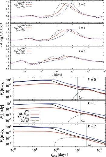
The radio light curves for the 2D simulations are shown by the black lines in the bottom panel of Figure 14. The counter-jet becomes visible as it turns sub-relativistic. For k = 0 this results in a clear bump-like feature in the light curve (as also shown by van Eerten & MacFadyen Reference van Eerten and MacFadyen2011). For larger k values, however, the jet decelerates and comes into view more gradually, causing only a mild flattening in the radio light curve that might be hard to discern when k = 2. Also shown in the bottom panel of Figure 14 are light curves for a spherical 1D simulation with the same true energy (orange lines), and for a double-sided cone of half-opening angle θ₀ taken from a spherical 1D simulation (from De Colle et al. Reference De Colle, Granot, Lopez-Camara and Ramirez-Ruiz2012a) with the same isotropic equivalent energy (blue lines). Late-time radio calorimetry usually assumes a spherical flow near the non-relativistic transition time t _NR (thick vertical grey lines), and is thus likely to consistently over-estimate the true energy by up to a factor of a few for k = 2, but either over-predict or under-predict it by a smaller factor for k = 0, 1 (as can be seen by comparing the orange and black lines in the figure).

5.1 Broadband modelling

Several groups have performed broadband modelling studies on samples of GRB afterglows including radio observations (e.g. Wijers & Galama Reference Wijers and Galama1999; Panaitescu & Kumar Reference Panaitescu and Kumar2001b; Reference Panaitescu and Kumar2002; Yost et al. Reference Yost, Harrison, Sari and Frail2003; Cenko et al. Reference Cenko2010; Reference Cenko2011). It is clear from these studies that the various modelling methods lead to different results for the same GRBs. Nonetheless, these efforts seem to indicate that there is a large spread in the physical parameters of the jet, the external medium, and collisionless relativistic shocks (see Figure 15). The top panel of Figure 15 shows the collimation corrected energies E _jet ~ 10⁵⁰ − 10⁵² erg versus the external medium number densities n ~ 10⁻³ − 10² cm⁻³ (for a uniform medium; k = 0) or A _* ~ 10⁻² − 10^−0.5 g cm⁻¹ (for a wind-like medium; k = 2). The jet initial half-opening angles θ₀ ranges from less than one degree up to tens of degrees.

Figure 15.

Top: The collimation corrected energy versus density for GRBs that have been modelled using their broadband radio, optical, and X-ray data (black symbols from Panaitescu & Kumar Reference Panaitescu and Kumar2002; grey symbols from Cenko et al. Reference Cenko2010, Reference Cenko2011). The densities are n in case of a homogeneous medium (solid symbols) and A _* in case of a stellar wind (open symbols). Middle: ε _e and ε _B for the same GRBs as in the top panel, plus those from Panaitescu (Reference Panaitescu2005) (black squares). Indicated are lines for ε _e = ε _B (equipartition) and ε _e = (ε _B )^1/2 (Medvedev Reference Medvedev2006). Bottom: The electron energy distribution power-law index p versus the density structure power-law index k, based on optical and X-ray spectra and light curves, for a sample of GRBs with good spectral and temporal coverage (Starling et al. Reference Starling2008; Curran et al. Reference Curran, Starling, van der Horst and Wijers2009).

The shock microphysical parameters are typically in the range ε _e ~ 10⁻² − 10⁻¹, ε _B ~ 10⁻⁵ − 10⁻¹, and p ~ 2 − 3. The middle panel of Figure 15 shows ε _e versus ε _B . Medvedev (Reference Medvedev2006) predicted a relation between these two parameters, ε _e ≈(ε _B )^1/2, based on physical arguments for a Weibel instability mediated relativistic collision shock in an electron-proton plasma. He had further argued that such a strong correlation is supported by the data, in particular the values of ε _e and ε _B inferred by Panaitescu (Reference Panaitescu2005). However, we do not find such a correlation, where the best fit data from Panaitescu (Reference Panaitescu2005) (or all the data shown in the middle panel of Figure 15) give a Spearman rank correlation coefficient of 0.12 (0.16) with a chance probability of 0.73 (0.42). We also show this predicted relation, as well as a linear one, for easier visual comparison with the inferred values.

Based on these results there does not seem to be universality in any of the parameters, also in the shock microphysics ones. Studies based on optical and X-ray light curves, and optical-to-X-ray spectra, can determine p and k, when making standard model assumptions. These studies confirm the non-universality of p, and also show that k varies between different GRBs, sometimes consistent with 0 (homogeneous medium) and not with 2 (wind-like medium), and vice versa (see bottom panel of Figure 15; Starling et al. Reference Starling2008; Curran et al. Reference Curran, Starling, van der Horst and Wijers2009). We note that these studies assume that we are viewing exactly along the jet symmetry axis (θ_obs = 0), which may have an effect mostly on the inferred values of k, because a non-negligible θ_obs can change the light curve slopes and k is determined by both the spectral and temporal slopes, while p is determined by the spectral slope alone.

While the instantaneous density in front of the shock as well as its energy and shock microphysics parameters can be determined from the instantaneous spectrum, the external density profile and in particular its power-law index k require such a modelling over a long time. However, in principal, the shock microphysics parameters might vary with time, which could have similar observational signatures and thus be degenerate with a different value of k, which is different than its true value. An important way to break such a degeneracy is through measuring the afterglow image size measurements. Such measurements could also help test the jet dynamics, and in particular its degree of lateral spreading (see Figure 16), although this is a bit challenging. Another way to probe the value of k is through its implications for the contribution of the counter-jet to the light curve, where k = 0 is expected to produce a pronounced late-time bump while k = 2 will only produce a very mild flattening, which might be hard to clearly observe (see upper panel of Figure 8). The time of a counter-jet bump would probe E/A (for an external density ρ_ext = AR ^−k ) since it scales as (E/A)^{1/(3 − k)} (with some dependence of the numerical coefficient on k and θ_obs, as can be seen in Figure 8).

Figure 16.

Fits of the evolution of the GRB 030329 VLBI image size up to 83 d (Granot et al. Reference Granot, Ramirez-Ruiz and Loeb2005a) with the later time size measurements over-plotted (Mesler et al. Reference Mesler, Pihlström, Taylor and Granot2012). In Model 1 there is significant lateral spreading during the trans-relativistic phase in the blast wave evolution, while in Model 2 there is no spreading until the non-relativistic phase.

We note, however, that there is not only a large spread in parameters obtained for different GRBs, but also a significant spread in parameters for individual GRBs obtained by different groups. Therefore, the shock microphysical parameters, or at least some of them, might potentially still be universal, at least at early enough times while the shock is still highly relativistic (Γ ≫ 1). Once the shock is no longer highly relativistic one might envision a dependence of the shock microphysics parameters on the shock Lorentz factor or its proper velocity. Furthermore, different assumptions or constraints on some of the parameters (e.g. the observing angle θ_obs or the microphysical parameters) can lead to significantly different values for the parameters, even if one uses the same method (van Eerten, van der Horst, & MacFadyen Reference van Eerten, van der Horst and MacFadyen2012; Leventis et al. Reference Leventis, van der Horst, van Eerten and Wijers2013). Studies involving decent sized samples (e.g. Panaitescu & Kumar Reference Panaitescu and Kumar2001b) indicate that there is indeed a spread in the parameters. Future modelling efforts of larger samples using one method and the same assumptions for all GRBs, and using more accurate modelling codes (van Eerten et al. Reference van Eerten, van der Horst and MacFadyen2012; Granot & Piran Reference Granot and Piran2012) should clarify how large this spread truly is.

5.2 A case study: GRB 030329

The GRB radio afterglow with the best spectral and temporal coverage by far is GRB 030329, with well-sampled radio light curves over two orders of magnitude in observing frequency (0.64 − 95 GHz), starting half a day after the initial trigger and still detectable a decade later (over almost four orders of magnitude in time). With these observations it has been possible to follow the evolution of the afterglow shock from the ultra-relativistic to the non-relativistic phase and perform detailed broadband modelling (see Figure 3; Berger et al. Reference Berger2003a; Frail et al. Reference Frail2005; Resmi et al. Reference Resmi2005; van der Horst et al. Reference van der Horst2005; Reference van der Horst2008). From all the modelling efforts, including those at optical and X-ray frequencies, two main interpretations have emerged.

One interpretation was that the GRB 030329 had a two-component jet (Berger et al. Reference Berger2003a) consisting of an initially very fast and fairly narrow jet (with θ₀ ~ 5°) contributing mostly to prompt γ-ray emission as well as the optical and X-ray light curves, and an initially slower and wider jet (with θ₀ ~ 17°) powering the radio light curves (a broadly similar model was also considered by Resmi et al. Reference Resmi2005; van der Horst et al. Reference van der Horst2008). In particular, Berger et al. (Reference Berger2003a) have attributed the sharp bump in the optical light curve that peaked at t ~ 1.5 d (Lipkin et al. Reference Lipkin2004) to the deceleration time of the wide jet component. However, it was later shown that the deceleration of a wider jet component cannot produce such a sharp feature in the light curve, and instead produces a much wider and smoother peak (Granot Reference Granot2005).

An alternative interpretation of the sharp bump in the optical light curve at t ~ 1.5 d, as well as a few additional bumps that are seen in the most detailed optical light curve up to several days (Lipkin et al. Reference Lipkin2004) are naturally explained as a series of refreshed shocks—slow shells that were ejected from the source early on (near the end of its prompt activity) that catch up with the afterglow shock at relatively late times, and inject energy into it (Granot, Nakar, & Piran Reference Granot, Nakar and Piran2003). This nicely explains the optical light curve and the relatively sub-energetic early γ-ray and X-ray emission. Moreover, the radio light curves appear to be very similar to the expectations from hydrodynamic simulations of a single initially uniform jet (see, e.g. the top panel of Figure 8), where the sharp break in their light curve can be attributed to the passage of ν _m , without requiring a second (wide) jet component.

Broadband modelling from radio to X-ray frequencies is challenging due to the many bumps in the optical light curves, but modelling of the radio light curves by themselves already provides good constraints on the physical parameters since the evolution of ν_sa, ν _m and the peak flux can be determined accurately. The physical parameters obtained by modelling only the early times, only the late times, and both at the same time, are consistent within a factor of a few even though the methods and assumptions are different for the various groups (see van der Horst et al. Reference van der Horst2008, for a discussion). The parameter with the largest spread, about one order of magnitude, is the external density, which is caused by the fact that it depends strongly on the precise values for ν_a and ν_m.

An important extra ingredient in the modelling of GRB 030329 are the VLBI size measurements, as discussed in Section 2.5.1. Granot et al. (Reference Granot, Ramirez-Ruiz and Loeb2005a) and Mesler & Pihlström (Reference Mesler and Pihlström2013) have performed combined modelling of the image size evolution and the light curves, and they find good agreement and again comparable physical parameters. As can be seen in Figure 16, the source size measurements favour a uniform ambient medium (k = 0) over a wind-like external density profile (k = 2) (Granot et al. Reference Granot, Ramirez-Ruiz and Loeb2005a), which has also been found by broadband modelling (van der Horst et al. Reference van der Horst2008; Mesler et al. Reference Mesler, Pihlström, Taylor and Granot2012). This result appears to be in contrast with the predictions for the emission coming from the counter-jet. The upper panel of Figure 8 or the bottom panel of Figure 14 show that in the case of a homogeneous medium (k = 0) there should be a bump or at least a clear flattening in the light curve at late times caused by emission coming from the counter-jet, while in the stellar wind case (k = 2) this is merely a mild flattening. This kind of bump has not been observed in the GRB 030329 light curves (Mesler & Pihlström Reference Mesler and Pihlström2013, see also the top right panel of Figure 1).

One possible way out of this apparent discrepancy is by relaxing the usual assumption that the counter-jet is intrinsically identical to the jet pointing towards us, and encounters a similar density and radial profile of the external medium. Although many astrophysical jet sources do show two jets, they are not necessarily identical or symmetrical. However, this is in most cases due to a double-sided AGN jet that is ejected quite symmetrically but interacts with different external density profiles on either side, at large distances from the source. On the other hand, the immediate environment of a GRB jet is very different, and it is less clear how reasonable is the required difference in external density, where the counter-jet should interact with an external density lower by a factor of several or more over at least a factor of a few in radius (assuming the two jets are intrinsically similar). More generally, the lack of a late-time rebrightening or flattening can provide constraints on the presence and properties of the counter-jet.

5.3 Newtonian transition: Shock microphysical parameters

The usual assumption that is made when modelling the synchrotron afterglow emission is that all electrons take part in a power-law energy distribution behind the shock. However, in general, the fraction ξ _e of electrons that take part in such a power-law distribution is expected to be less than unity, where the bulk of the electrons form a relativistic Maxwellian, as their energy distribution is thermalised behind the shock (e.g. Eichler & Waxman Reference Eichler and Waxman2005; Giannios & Spitkovsky Reference Giannios and Spitkovsky2009). In particular, particle in cell simulations suggest that ξ _e can be as low as a few percent (Spitkovsky Reference Spitkovsky2008a; Martins et al. Reference Martins, Fonseca, Silva and Mori2009). The minimal electron Lorentz factor of the power-law energy distribution, γ _m , and its average Lorentz factor 〈γ _e 〉, are given (for p > 2) by

(4) \begin{equation} \gamma _m = \frac{p-2}{p-1}\langle {\gamma _e}\rangle = 1 + \frac{p-2}{p-1}\frac{\epsilon _e}{\xi _e}\frac{m_p}{m_e}(\Gamma _{12}-1)\ , \end{equation}

$\Gamma _{12}-1\approx \frac{1}{2}\beta _{12}^2$

(5) \begin{equation} \gamma _m-1 \approx \frac{p-2}{p-1}\frac{\epsilon _e}{\xi _e}\frac{m_p}{m_e}\left(\frac{\beta _{12}^2}{2}\right) = \frac{g\epsilon _{e,-1}}{\xi _e}\left(\frac{\beta _{12}}{0.18}\right)^2\ , \end{equation}

(6) \begin{equation} \beta _{12} < \beta _{\rm cr} = 0.18\sqrt{\frac{\xi _e}{g\epsilon _{e,-1}}}\ . \end{equation}

Once β₁₂ drops below the critical value of β_cr, the usual assumptions of a constant ξ _e and ε _e must break down. Granot et al. (Reference Granot2006) have considered, in the context of the radio afterglow from the giant flare of SGR 1806 − 20 (e.g. Gaensler et al. Reference Gaensler2005), the plausible scenario in which ε _e remains constant while ξ _e starts decreasing from its previous value (which is assumed to be constant) in such a way that γ _m ≈2 is maintained, i.e. ξ _e = gε _e,−1(β₁₂/0.18)²∝β² ₁₂. For an external density that scales as R ^−k and a spherical Newtonian flow, ξ _e ∝β² ₁₂∝R ^k−3∝t ^{−2(3−k)/(5−k)}.

For a uniform external density, the resulting flux decay rate in the most relevant power-law segment of the spectrum for late-time radio observations (PLS G in Figure 2) is F _ν∝ν^(1−p)/2 t ^−3(p+1)/10 (Granot et al. Reference Granot2006), while more generally F _ν∝ν^(1−p)/2 t ^{−3(p+1)/[2(5 − k)]}. This decay rate is significantly shallower for a uniform external medium (but somewhat steeper for a wind-like external medium with k = 2 for p < 3) compared to that for the usual assumptions made in GRB afterglow modelling at the Newtonian regime, which gives F _ν∝ν^{(1 − p)/2} t ^{−[3(5p−7)−2k(2p−3)]/[2(5−k)]}. For the radio afterglow of the giant flare from SGR 1806 − 20, for which p≈2.5 was inferred from the observations and a uniform external medium (k = 0) is expected, this predicts F _ν∝t ^−1.05 (Granot et al. Reference Granot2006), which is in very good agreement with the observed t ⁻¹ − t ^−1.1 at late times (Gelfand et al. Reference Gelfand2005). This effect was recently also pointed out in the context of late-time GRB radio afterglows (Sironi & Giannios Reference Sironi and Giannios2013). In general, such late-time radio observations from GRBs, SGR giant flares, or other synchrotron emitting shocks that gradually decelerate from mildly relativistic to Newtonian speeds can help investigate the shock microphysics in this intriguing transition regime.

6.1 New instrumentation

Although we have learned a lot about GRB jets from radio observations, there are still several open questions for which a new generation of radio observatories could provide answers. There is a large international effort to build the Square Kilometer Array this decade, which will revolutionise radio astronomy. Many precursor telescopes are being built, commissioned, or are already operational: the Australian Square Kilometer Array Pathfinder (ASKAP; 0.7 − 1.8 GHz; Johnston et al. Reference Johnston2008); MeerKAT in South-Africa (0.58 − 14.5 GHz, but not continuous frequency coverage; Booth & Jonas Reference Booth and Jonas2012); the Low Frequency Array (LOFAR; 10 − 240 MHz; van Haarlem et al. Reference van Haarlem2013), with the core in The Netherlands but stations in several European countries; the Murchison Widefield Array (MWA; 80 − 300 MHz; Tingay et al. Reference Tingay2013) in Australia; and the Long Wavelength Array (LWA; 10 − 88 MHz; Ellingson et al. Reference Ellingson2013) in the USA. Transient sources, including GRBs, are among the key science objectives for all these observatories. Besides these new facilities, several others that have been pivotal in GRB research up to now have been upgraded, or are in that process: the VLA upgrade, the focal-plane array system Apertif on WSRT, AMI as the Ryle Telescope upgrade, the new back-ends of the ATCA and the Very Long Baseline Array (VLBA), and also the increasing use of e-VLBI providing real-time data transfer and processing. All these new and upgraded facilities will not only explore a larger spectral range, going down to the lowest frequency radio wave passing through the Earth's atmosphere, but also will provide improved sensitivities, bandwidth, and spatial, spectral and temporal resolution. These improvements will be important for advancing our understanding of GRB jet physics in several ways.

First of all the improved sensitivity, in particular for the VLA, will have a big impact on the number of detected GRBs and significantly increase the sample size. A few years of observations with the upgraded VLA should be able to make it clear whether the current sample is indeed sensitivity limited (Chandra & Frail Reference Chandra and Frail2012) or if there are two distinct populations of GRB radio afterglows (Hancock et al. Reference Hancock, Gaensler and Murphy2013). The number of GRBs with well-sampled radio light curves for broadband modelling to determine the physical parameters is expected to increase significantly, not only by observing deeper in terms of sensitivity but also over a larger frequency range. Especially late-time, low-frequency observations will be important for performing true radio calorimetry, years or even decades after the GRB trigger (van der Horst et al. Reference van der Horst2008).

Another significant improvement in observational capabilities over the last few years is that the radio regime has entered time-domain astronomy. Several phenomena are delayed at radio frequencies compared to optical or X-rays, but there is also part of the observational parameter space that has not been explored until recently, in particular the first minutes to hours after a GRB trigger. AMI 15 GHz follow-up of Swift triggers, with sub-mJy sensitivity levels, did result in the earliest detection of a long GRB at radio frequencies, GRB 130427A, within 8 h after the burst of γ-rays (Anderson et al., in preparation). A couple of months later the earliest radio detection of a short GRB was found at the same timescale with the VLA, namely GRB 130603B (Fong et al. Reference Fong2013). Besides searches at the traditional radio frequencies, there are also efforts ongoing at low radio frequencies, for instance with LOFAR, MWA and LWA, to search for early-time, possible prompt coherent emission. Detections of, or limits on, such emission could provide an important clue for the jet production and collimation mechanisms.

6.2 VLBI prospects

Crucial for theoretical and modelling efforts are matching observational efforts. Of particular value are direct source size measurements with VLBI, putting independent constraints on the physical parameters and possibly probing the jet structure directly. The process of e-VLBI (Conway Reference Conway2009), which allows near-realtime VLBI observations, has enabled significantly faster follow-up of transients than traditional VLBI. Although it is logistically difficult to organise global e-VLBI observations, this is technically feasible and should be possible in the near future. Although the combined radio brightness and proximity of GRB 030329 has been unique so far, the observational advances that have been made over the last years put us in a great position to study a similar event in even better detail when it occurs. Such a study could be improved by VLBI at higher radio frequencies, thus achieving even better resolution, or with Space VLBI, as demonstrated by the observations performed with the VLBI Space Observatory Programme (VSOP; Hirabayashi et al. Reference Hirabayashi2000) and RadioAstronFootnote ³ . Although in Space VLBI the sensitivities and data rates are currently limited, this is certainly an interesting prospect for future high-resolution observations.

In the context of time-domain astronomy, it is now also feasible to trigger e-VLBI observations at similar timescales as with the ‘regular’ radio telescopes. Although measuring the GRB source size is not expected at that time yet, such observations with for instance the European VLBI Network (EVN) or VLBA are still very useful. In particular, they will not only provide deep observations with good sensitivity, but could also distinguish early on between GRB emission from a faint AGN or radio emission from star formation in the host galaxy (which will be resolved out with VLBI). Moreover, they can produce an early accurate location of the flux centroid, that could be used to constrain the proper motion at later epochs. VLBI can also play an important role in time-domain searches, due to better sensitivity than single dish telescopes, and also because the various telescopes in the VLBI arrays have different radio frequency interference (RFI) environments and different back-end systems, making it easier to identify events that are not astrophysical in nature.

6.3 Modelling and numerical simulations

All the aforementioned observational improvements tie in perfectly with the improved broadband modelling efforts. Recently is has become possible to directly fit hydrodynamic simulations including detailed emission calculations to broadband light curves (van Eerten et al. Reference van Eerten, van der Horst and MacFadyen2012), which enables taking into account effects that are not accounted for (properly) in most analytical models, for instance the jet orientation with respect to the observer (Granot et al. Reference Granot, Miller, Piran, Suen, Hughes, Costa, Frontera and Hjorth2001; Reference Granot, Panaitescu, Kumar and Woosley2002; van Eerten & MacFadyen Reference van Eerten and MacFadyen2012; De Colle et al. Reference De Colle, Ramirez-Ruiz, Granot and Lopez-Camara2012b) and the delayed jet break at radio frequencies due to synchrotron self-absorption (van Eerten et al. Reference van Eerten, Meliani, Wijers and Keppens2011). At the same time, new physically derived analytical models, both analytic jet models (Granot & Piran Reference Granot and Piran2012) or analytic spherical models calibrated to hydrodynamic simulations (Leventis et al. Reference Leventis, van der Horst, van Eerten and Wijers2013) are available for broadband modelling now. With the increased sample of broadband data sets and more accurate modelling efforts, it will be possible to better determine the physical parameters and constrain the jet lateral spreading.

More generally, there is a steady improvement in the capabilities of numerical simulations also to study earlier phases in the jet dynamics. This includes the launching of the jet using general relativistic MHD simulations from an accretion disc around a rotating black hole (e.g. Koide et al. Reference Koide, Meier, Shibata and Kudoh2000; Nishikawa et al. Reference Nishikawa2005; McKinney Reference McKinney2006; Krolik & Hawley Reference Krolik and Hawley2010; Tchekhovskoy & McKinney Reference Tchekhovskoy and McKinney2012; McKinney, Tchekhovskoy, & Blandford Reference McKinney, Tchekhovskoy and Blandford2012) or from the merger of two neutron stars (e.g. Liu et al. Reference Liu, Shapiro, Etienne and Taniguchi2008; Rezzolla et al. Reference Rezzolla2011; Shibata et al. Reference Shibata, Suwa, Kiuchi and Ioka2011; Palenzuela et al. Reference Palenzuela2013) or a neutron star and a black hole (Chawla et al. Reference Chawla2010; Etienne et al. Reference Etienne, Liu, Paschalidis and Shapiro2012; Etienne, Paschalidis, & Shapiro Reference Etienne, Paschalidis and Shapiro2012), as well as jet formation and propagation inside the progenitor star of a long-soft GRB, also in special relativity and both for a collapsar (e.g. Nagataki Reference Nagataki2009; Harikae, Takiwaki, & Kotake Reference Harikae, Takiwaki and Kotake2009) and for a millisecond magnetar (e.g. Komissarov & Barkov Reference Komissarov and Barkov2007; Bucciantini et al. Reference Bucciantini, Quataert, Arons, Metzger and Thompson2008; Reference Bucciantini, Metzger, Thompson and Quataert2012). These simulations have put those models for the central engine on much firmer ground, and may help test their predictions against observations.

What is more, these earlier stages of the jet dynamics are what set the stage, or determine the initial conditions for its late-time evolution during the afterglow, which directly affects the afterglow broadband modelling. There has been significant progress also in the numerical studies of the jet's late time evolution (see Section 4.4). Such numerical simulations could improve the accuracy of late-time radio calorimetry. The great improvements in the simulations of the different stages in the jet dynamics may soon make it feasible to simulate the jet dynamics within a single simulation from close to the source, well within its progenitor star (for long GRBs) as it breaks out of the star, is eventually decelerated by the external medium and finally becomes sub-relativistic and approaches the Sedov-Taylor solution. Since at present it is possible to simulate the jet dynamics only one stage at a time, such a unification of the different stages could lead to great progress, and more firmly relate the properties of the central source and the jet launching, collimation, acceleration and composition, to the observational signatures as manifested in the GRB prompt emission and afterglow.

Moreover, there has been considerable progress in our understanding of collisionless shock physics, largely thanks to particle in cell simulations, both in the relativistic regime (Spitkovsky Reference Spitkovsky2008a; Reference Spitkovsky2008b; Chang, Spitkovsky, & Arons Reference Chang, Spitkovsky and Arons2008; Martins et al. Reference Martins, Fonseca, Silva and Mori2009; Keshet et al. Reference Keshet, Katz, Spitkovsky and Waxman2009; Sironi & Spitkovsky Reference Sironi and Spitkovsky2009a; Reference Sironi and Spitkovsky2009b; Nishikawa et al. Reference Nishikawa2009; Frederiksen et al. Reference Frederiksen, Haugbølle, Medvedev and Nordlund2010; Sironi & Spitkovsky Reference Sironi and Spitkovsky2011; Sironi, Spitkovsky, & Arons Reference Sironi, Spitkovsky and Arons2013), as well as in the mildly relativistic (e.g. Murphy et al. Reference Murphy, Dieckmann, Bret and Drury2010) or Newtonian (e.g. Amano & Hoshino Reference Amano and Hoshino2007; Kato & Takabe Reference Kato and Takabe2008; Amano & Hoshino Reference Amano and Hoshino2009; Reference Amano and Hoshino2010; Riquelme & Spitkovsky Reference Riquelme and Spitkovsky2011; Gargaté & Spitkovsky Reference Gargaté and Spitkovsky2012) regimes. This has already contributed greatly to the field, and is likely to continue to do so for time to come. All these numerical efforts naturally go hand in hand with the analytic work on these topics, and a symbiotic relation has already greatly contributed to the progress in the field, and is expected to do so in the future as well. Keep in mind that the state of the art knowledge on shock microphysics when modelling the afterglow observations is important in order to get the most out of the data, and try to test the theoretical predictions.

6.4 Testing the theory with observations