


1. Introduction
Fused Filament Fabrication (FFF) is widely used in both research and industry. The environmental impact and manufacturing effort are dominated by two factors – first is the duration of the printing process and second is the amount of material required for the part and its support structures. Literature consistently identifys print time and material consumption as the primary drivers of resource use (Reference Kokare, Oliveira and GodinaKokare et al., 2023; Reference Sola, Rosa and FerrariSola et al., 2024). Print time increases mainly with layer count and nozzle travel, while material consumption is driven by solid volume and required supports. To estimate manufacturing complexity, it is therefore common practice to determine the printing effort required based on time-dependent and material-dependent drivers (Reference Enemuoh, Duginski, Feyen and MentaEnemuoh et al., 2021; Reference Harding, Griffiths, Rees and PletsasHarding et al., 2023). In particular, support generation is widely recognized as a major effort and sustainability lever because it directly adds material, time and energy waste (Reference Fazla, Dilberoğlu, Yaman and DölenFazla et al., 2021; Reference Jiang, Xu and StringerJiang et al., 2018).
Consequently, many geometric decisions made early in the design process directly influence printing effort. Designers often explore numerous variants of a part before committing to process parameters, but evaluating the printing effort for each variant through full slicing runs is time-consuming. This is further amplified by build orientation, which can strongly affect support demand, surface quality, and build time, and therefore represents a key manufacturing decision rather than a purely geometric detail (Reference Di Angelo, Di Stefano and GuardianiDi Angelo et al., 2020).
Existing approaches for estimating manufacturing complexity provide only partial support in early design stages. Many methods analyze printability or geometric feasibility (Reference Fudos, Ntousia, Stamati, Charalampous, Kontodina, Kostavelis, Tzovaras and BilalisFudos et al., 2021). For example, geometry-based toolboxes can flag common printability issues such as warping, toppling, surface quality risks, or problematic overhang-related features (Reference Budinoff and McMainsBudinoff & McMains, 2021). Others introduce geometric complexity measures that are used qualitatively, for example as one of several criteria in process selection for hybrid manufacturing (Reference Joshi and AnandJoshi & Anand, 2017). In addition, early-stage screening methodologies have been proposed to identify suitable AM candidates already in conceptual design (Reference Lindemann, Reiher, Jahnke and KochLindemann et al., 2015). However, such indicators are rarely calibrated against an empirical effort metric tailored to FFF, and they typically do not quantify how much more (or less) manufacturing effort one geometry requires compared to a suitable reference. As a result, designers currently lack a simple, geometry-only indicator that (i) approximates the relative manufacturing effort of a part and (ii) expresses this effort on a scale that is consistent across different geometries.
This paper addresses this need by introducing a geometry-based complexity factor that predicts the relative manufacturing effort of a part in FFF. The factor depends solely on the part geometry, making it suitable for early design stages, and is calibrated against an effort measure derived from print time and material consumption. Each part is compared to a volume-equivalent reference cube, which provides a neutral baseline for assessing additional effort caused by geometric complexity.
The approach determining the complexity factor follows a four-step workflow. First, a large and heterogeneous corpus of STL models is sliced with a fixed FFF profile to obtain reference values for print time and material consumption for each part and its volume-equivalent cube. Second, a set of dimensionless geometric metrics is computed directly from the STL mesh. These metrics describe overhangs, support requirements, footprint characteristics, island formation, thin walls, surface-to-volume excess, slenderness, and layer-count. Third, a constrained linear index model is fitted to relate these geometric metrics to the normalized effort values. Finally, a monotonic scale adjustment refines the index while preserving its rank order. The resulting complexity factor provides a fast and interpretable estimate of relative manufacturing effort and reduces the number of slicing operations required in early design stages.
In summary, the paper presents a geometry-based complexity factor for FFF, calibrates it on a large sliced dataset, and evaluates its predictive performance and interpretability for use in early design decisions.
2. Methodology
This section details how the complexity factor is defined and calibrated following the four-step workflow introduced above. It describes the generation of the reference effort from sliced parts and volume-equivalent cubes, the transformation into the normalized target variable, the geometric metrics extracted from STL meshes, the constrained index model with regularization and monotonic scaling, and the validation protocol (train–test split, cross-validation, performance metrics, bootstrapping, and ablation). Figure 1 provides a visual overview of this methodology.
Overview of the calibration workflow. Input STLs are processed in two parallel paths to extract the target variable
 (from slicing effort) and the geometric metrics
 (from mesh analysis). Both are used to calibrate the final complexity factor


Figure 1 Long description
A diagram illustrating the calibration workflow for estimating manufacturing complexity in Fused Filament Fabrication. The diagram is structured into several labeled sections. At the top, Data Input is shown with a Heterogeneous STL Corpus consisting of 3,557 parts. This input is split into two parallel paths. On the left, Reference Effort is calculated through slicing the part and cube, calculating E_total at 50/50, and performing a 3-step transformation to derive the target variable y. On the right, Geometry Analysis involves analyzing the mesh, extracting 8 metrics, and applying linear scaling to obtain scaled metrics k_i. These paths converge at Model Input, where y and k_i are used in a constrained linear model to find weights w_i. This is followed by monotonic scale adjustment g, leading to the Final Complexity Factor KF at the bottom of the diagram.
2.1. Reference effort generation
The complexity factor is intended to predict how demanding a part is to print, using only its geometry as input. To calibrate such a geometry-based model, we first need a reference quantity that measures printing effort in a consistent way. This quantity should combine print time and material consumption and make parts of different shapes and sizes comparable. We refer to this quantity as reference effort. It expresses how much more or less printing effort a part requires compared to a simple reference geometry with the same volume. The reference effort combines predicted print time and filament mass into a single relative measure and later serves as the basis for the target variable used in the calibration of the complexity factor. In other words, it indicates whether a given geometry is easier or harder to print than a neutral baseline.
As input data we use the STLs_1 subset of the Slice-100K dataset of triangulated models for extrusion-based 3D printing (Reference Jignasu, Marshall, Mishra, Rillo, Ganapathysubramanian, Balu, Hegde and KrishnamurthyJignasu et al., 2024). This subset contains roughly 5,000 STL models and serves as the starting point for our analysis. From these models, all parts that exceed the build volume or have a non-watertight mesh are removed. After this filtering step, 3,557 valid parts remain and form the dataset used for calibration and evaluation.
All parts are processed with Bambu Studio in command-line mode (version 2.2.1.60) using a fixed profile for a Bambu X1 Carbon printer. The profile uses a 0.4 mm nozzle, Bambu PLA Basic filament (density 1.26 g/cm3, diameter 1.75 mm), a layer height of 0.20 mm, three outer walls, four bottom solid layers, five top solid layers, and a grid infill density of 15 %. Machine, process, and filament settings are kept constant for all runs. The study assumes a conventional single-axis FFF process with a fixed build direction and single-nozzle extrusion. Transfer to substantially different configurations (e.g., multi-axis or multi-nozzle systems) is not considered and would require new reference data. Multi-axis material-extrusion approaches have been demonstrated to reduce or even avoid support structures for overhanging features, which would change the effort drivers considered in this study (Reference Han, Wu, Liu, Li, Song and CuiHan et al., 2025). Build orientation is treated as user-defined and fixed, as it is typically chosen to satisfy functional and quality requirements rather than being optimized solely for sustainability. Each STL model is sliced in two variants. In the first variant, support structures are enabled with a support overhang threshold of 45° and automatic tree-support generation. In the second variant, the same parameters are used but support structures are disabled. The part mass is taken from the variant without supports. The support mass is computed as the difference between the total mass with supports and the part mass without supports. The print time is taken from the support-enabled variant. All slicing results are read from the metadata stored in the 3MF container (slice_info.config).
For each part with volume
 , a volume-equivalent reference cube is defined. Its edge length a is obtained from the part volume as shown in Equation (1). The reference cube is sliced without supports using the same profile. It provides a neutral baseline with identical material and process settings and the same volume as the part.

Based on the slicing results, two partial effort factors are defined for each part. The time-based factor compares the predicted print time of the part to that of its reference cube, as given in Equation (2). The material-based factor compares the corresponding filament masses, as given in Equation (3).


Both components are treated equally and combined into a total effort factor according to Equation (4).

Values of the total effort
 greater than one indicate that the part requires more time and material than its volume-equivalent cube, while values below one indicate a more efficient geometry. This total effort serves as the starting point for the target variable defined in Section 2.2.
2.2. Definition and transformation of the target variable
For the calibration of the complexity factor, we require a scalar target variable
 that quantifies the printing effort of each part. This target is derived from the total effort
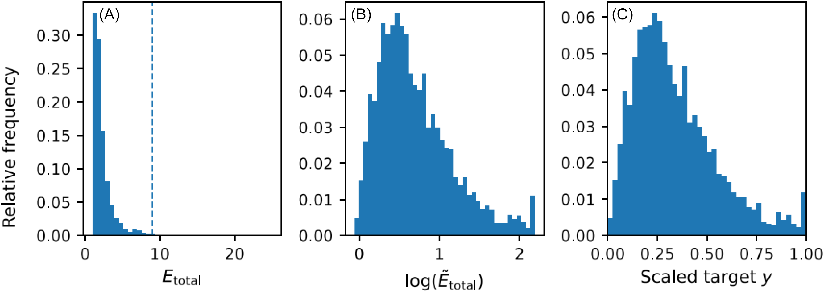
 defined in Section 2.1. When inspecting the distribution of
 , most parts lie in a moderate range, but a small number have much larger values. This creates a long right tail in the distribution. In addition, some parts have
 because they require less time and material than the reference cube. To obtain a stable and comparable target variable for regression,
 is transformed into a normalized scalar variable
 in three steps.
In the first step, extreme outliers are limited by clipping at the 99th percentile of the training data. Let
 denote this threshold. The clipped effort
 is defined as in Equation (5). For most parts
 is identical to
 . Only values above the 99th percentile are reduced to this threshold.

In the second step, the clipped effort
 is compressed by a logarithmic transformation to reduce scale differences between low and high effort values. A small constant
 is added for numerical stability. The transformed variable
 is defined in Equation (6).

In the third step, the log-transformed values
 are linearly mapped to the interval
 . The minimum and maximum of the log-transformed training data,
 and
and
 are used as scaling parameters, as shown in Equation (7). Values outside this range are limited to zero or one. The scaling parameters are derived from the training data only and then applied unchanged to the test data to avoid information leakage.

The resulting variable
 is used as the target variable for the complexity factor model described in Section 2.4. The transformation is strictly monotonically increasing in
 , so higher effort always leads to a higher value of
 (Figure 2). In the present dataset, the 99th-percentile clipping affects 36 out of 3,557 samples (1 %), limiting the influence of rare extreme outliers while leaving the vast majority of the distribution unchanged. Parts with
 remain valid and correspond to particularly efficient geometries on the lower end of the target scale.
Distribution and transformation of the total effort. (A) histogram of total effort
 with the 99th-percentile clipping threshold; (B) log-transformed distribution; (C) scaled target
 ; heavy tails are clipped, log-compressed, and linearly scaled

2.3. Geometric metrics
The complexity factor is built from geometric metrics that are computed directly from the STL mesh. The selection follows Design for Additive Manufacturing (DfAM) reviews, which highlight geometry-dependent aspects of printability such as overhangs, thin walls, support-related features, build-plate adhesion, layer topology, surface complexity, global aspect ratio, and build length (Reference Alfaify, Saleh, Abdullah and Al-AhmariAlfaify et al., 2020; Reference Pradel, Zhu, Bibb and MoultriePradel et al., 2018). All metrics are defined as dimensionless quantities in the interval
 . Higher values indicate geometries that are expected to be more demanding to print. The following metrics k
1 to
. Higher values indicate geometries that are expected to be more demanding to print. The following metrics k
1 to
 are used:
-
• Overhang ratio (k 1): measures the proportion of surface area whose outward normal forms an angle greater than 45° with the build-plate normal. Such regions are typically difficult to print without supports and tend to reduce surface quality. The metric captures geometric overhangs independent of local bridge length. Short unsupported spans that do not require support are accounted for separately through the support requirement metric
 , which incorporates a bridging-length threshold.
 -
• Footprint area (k 2): captures the effective contact area between the part and the build plate. It is derived from the cross-section in the first non-empty layer and normalized with respect to the projected bounding box of the part. No absolute thresholds are used to define “small” or “large” footprints. The metric is interpreted relative to the dataset and normalized through the common training-set scaling described below. Small effective footprints increase the risk of adhesion failures, while very large footprints can promote residual stresses and warping. Less favorable footprints lead to higher values of k 2.
-
• Island formation (k 3): describes interruptions within individual layers. For each layer, all disconnected cross-sectional regions are identified. The area of all regions except the largest is treated as island area. The metric k 3 is given by the average ratio of island area to total layer area across all layers. Frequent or large islands lead to more non-productive travel moves, retractions, and changes in printing direction.
-
• Thin walls (k 4): is derived from a sampled wall-thickness distribution. Local wall thickness is estimated by ray casting from surface points into the mesh and compared to a reference threshold of twice the line width. Parts that contain very narrow features obtain higher values of k 4 and are more prone to printing instabilities and local defects.
-
• Surface-to-volume excess (k 5): compares the surface-to-volume ratio of the part to that of a mass-equivalent cube. Higher values indicate a relatively large surface area for the available volume, which implies longer contour paths and more travel distance per unit of deposited material.
-
• Slenderness (k 6): is defined as the ratio of the part height to the smaller base dimension of its bounding box. A saturation factor limits the metric once the aspect ratio exceeds a given threshold. High values of k 6 correspond to tall, narrow parts that are more susceptible to vibration, deflection, and layer-wise instabilities during printing.
-
• Layer-count ratio (k 7): compares the number of layers required to build the part at the given layer height to the layer count of a volume-equivalent cube. Geometries that require more layers than the baseline receive higher values of k 7, reflecting the additional nozzle travel distance and print time.
-
• Support requirement (k 8): estimates how much of the material in each layer is not backed by material in the layer below. A bridging-length threshold is used to account for limited unsupported span lengths. This metric complements the overhang ratio by focusing on unsupported regions that arise from the layer-by-layer topology rather than from local surface orientation alone.

All geometric metrics are computed from the STL geometry. Each metric is then scaled linearly to the interval
 based on the minimum and maximum values observed in the training set. The same scaling parameters are applied to the test set, and values outside the observed range are capped at zero or one. The resulting normalized metrics serve as input features to the index model described in Section 2.4.
2.4. Modeling the complexity factor
This section describes the index model, constraints, regularization, and subsequent scale adjustment. The goal is an understandable and stable complexity factor calculated solely from geometric metrics.
The complexity factor originates as a linear raw index. For a part with metrics
 , the raw index is defined as shown in Equation (8).

The variables k
i
represent the normalized geometric metrics described in Section 2.3,
 are their corresponding weights, and
 is the intercept. The estimated raw index
 expresses the predicted geometric complexity before scaling.
To ensure technical plausibility and comparability, three constraints are applied:
-
• Non-negativity:
for all
(Increased difficulty cannot decrease the effort) -
• Scale Normalization:
(Fixes the index’s unit, enabling comparisons) -
• Intercept Bound:
(Prevents b from dominating the index, chosen data-driven)


The parameters
 and
and
 are estimated by fitting the raw index to the target variable
 defined in Section 2.2 using least squares under the constraints above. The optimization problem is formulated as shown in Equation (9).

Here
 denotes the normalized target value of part
 and
and
 the value of metric
 for that part. To stabilize the model when metrics are correlated, weak regularization is applied. It pulls the weights toward a uniform distribution as shown in Equation (10).

The parameter
 controls the regularization strength and is selected, together with
 , by cross-validation on the training set as described in the calibration protocol.
In a second step, a strictly monotonic piecewise-linear calibration function
 is learned to correct remaining scale distortions while preserving the rank order. The adjusted complexity factor is given in Equation (11). Because
 is monotonically increasing, parts with a higher raw index always receive a higher calibrated value.

The optimization problem is convex and deterministic, guaranteeing a unique global solution for given hyperparameters. Details of the calibration and evaluation procedure, including the train–test split and cross-validation, are given in Section 2.5.
2.5. Calibration and validation protocol
The complexity factor model is calibrated and evaluated on a held-out test set. The data are split into training and test sets in an 80/20 proportion using stratification, so that the distribution of the target variable y is preserved. All preprocessing steps, including clipping and scaling of the target and metrics, are fitted on the training set and then applied unchanged to the test set to avoid information leakage. The reported performance therefore reflects generalization within the fixed process assumptions of the chosen profile (layer height, infill, wall counts) and the selected printer and material combination. Transfer to substantially different profiles can be assessed by re-running the same calibration protocol with new reference slicing data. The workflow is implemented in Python using common scientific libraries such as NumPy, pandas, and scikit-learn.
The hyperparameters
 and
and
 are selected on the training set by five-fold cross-validation, optimizing the mean absolute error (MAE). For each candidate pair (
 ,
,
 ), the constrained and regularized index model described in Section 2.4 is fitted and evaluated in the cross-validation. After selecting the best hyperparameter combination, the model parameters and the monotonic calibration function
 are refitted on the full training set.
Model performance is reported on the held-out test set. We use the coefficient of determination
 2, the mean absolute error (MAE), and Spearman’s rank correlation coefficient to characterize the agreement between predicted and observed values of
 . Weight stability is assessed by bootstrap resampling of the training data. We draw
 bootstrap samples with replacement, fit the model on each resample, and summarize the resulting weight distributions by their median and 95 % intervals. The relevance of individual metrics is evaluated through ablation studies, in which the model is refitted with one metric removed and the resulting increase in MAE on the test set is recorded.
3. Results
This section presents the results obtained with the calibrated complexity factor. We first report the predictive performance on the held-out test set and the quality of the calibration. We then summarize the estimated weights of the geometric metrics and their stability. Finally, we analyze the relevance of individual metrics using an ablation study.
3.1. Test performance and calibration
The calibrated index exhibits a strong monotonic relationship with the target variable
 on the held-out test split and is well calibrated across most of the range (Figure 3). The scatter plot of predicted complexity versus target values shows a dense concentration of points around the identity line, and the binned averages follow the diagonal closely, with error bars indicating 95 % confidence intervals (CI). Deviations are mainly observed in the uppermost bins, where only few parts are present, which explains the larger variance in this region.
Test performance and calibration; predicted complexity
 versus target
 on the test set; the dashed line shows the identity; orange markers show binned means with 95 % confidence intervals (CI)

On the test set, the model achieves a coefficient of determination R
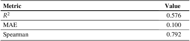
2 of 0.576, a mean absolute error (MAE) of 0.100, and a Spearman rank correlation of 0.792 (Table 1). These values indicate that the ranking of parts is reproduced reliably and that the average deviation on the normalized
 scale is around ten percentage points. In particular, Spearman’s rank correlation reflects how reliably the model preserves the relative ordering of parts by effort, which is the primary requirement for early screening. The hyperparameters selected in the calibration protocol lead to a regularized model with
 and an intercept at the lower bound
 , so that the index is fully determined by the geometric metrics.
Performance metrics on the test set (R 2, MAE, Spearman)

3.2. Weights of the complexity factor and stability
The estimation yields an intercept
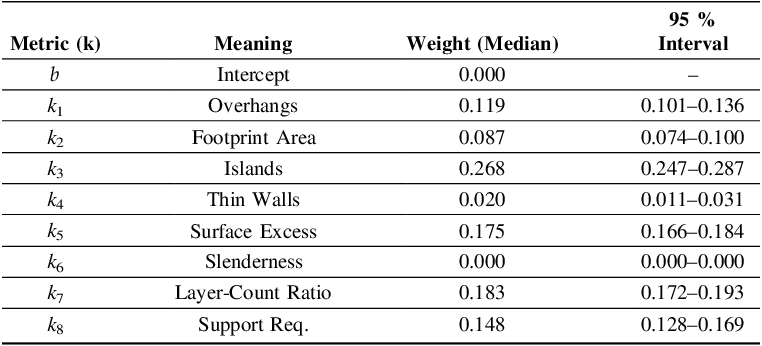
 and a set of nonnegative weights for the eight geometric metrics (Table 2). Island formation (k
3), layer-count ratio (k
7), and surface-to-volume excess (k
5) receive the largest weights, while overhang ratio (k
1), support requirement (k
8), and footprint area (k
2) play a secondary but non-negligible role. Thin walls (k
4) receive a small positive weight, and slenderness (k
6) is assigned to a weight of zero.
and a set of nonnegative weights for the eight geometric metrics (Table 2). Island formation (k
3), layer-count ratio (k
7), and surface-to-volume excess (k
5) receive the largest weights, while overhang ratio (k
1), support requirement (k
8), and footprint area (k
2) play a secondary but non-negligible role. Thin walls (k
4) receive a small positive weight, and slenderness (k
6) is assigned to a weight of zero.
Final weights with 95 % intervals (bootstrap,
 )
)

Bootstrap resampling with
 samples confirms that the estimated weights are stable. The median weights and their 95 % bootstrap intervals are narrow for the dominant metrics and do not overlap with zero (Table 2). The zero weight for slenderness is also robust under resampling, which suggests that this metric does not contribute additional explanatory power beyond the other geometry descriptors for the parts and process settings studied here.
3.3. Metric relevance and ablation
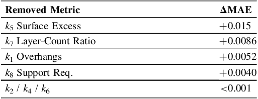
The ablation study quantifies the impact of each metric on predictive performance. For each metric in turn, the model is refitted on the training data without this metric and evaluated on the test set. The resulting increase in mean absolute error
 is reported in Table 3.
Change in error during ablation (Δ MAE, Test)

Removing the surface-to-volume excess (k 5) yields the largest increase in error, followed by the layer-count ratio (k 7) and the overhang ratio (k 1). The support requirement (k 8) also leads to a measurable increase when omitted. In contrast, removing footprint area (k 2), thin walls (k 4), or slenderness (k 6) changes the MAE by less than one thousandth. This pattern is consistent with the learned weights and supports the interpretation that k 3, k 5, and k 7 form the core of the index, while k 1 and k 8 provide additional but smaller corrections. This ablation experiment is purely diagnostic and is not intended as a recommendation to omit individual metrics in practice. Instead, the increase in error serves as a sensitivity measure for the relative contribution of each metric.
Overall, the results show that the complexity factor can reproduce the relative ordering of printing effort across parts with reasonable accuracy and that a small subset of geometric metrics dominates the prediction.
4. Discussion
The results show that a pure geometry index can reliably rank the relative manufacturing effort in FFF. The strong rank correlation (
 ) supports its suitability for early screening phases, while the moderate deviation (
 ) reflects the expected limit of an estimation made without slicer information.
The main value of the model lies in the interpretation of its weights, which are statistically stable and consistent with process logic. While nonlinear models could capture interactions between geometric features, they typically reduce transparency and interpretability. The present work therefore deliberately adopts a linear and constrained formulation to preserve direct attribution of effort to individual geometric drivers. Three drivers stand out: k 3 (islands), k 7 (layer-count ratio), and k 5 (surface-to-volume excess). This is a plausible outcome, because these metrics capture inefficient aspects of the FFF process. Islands lead to unnecessary travel paths and retractions, while high surface-to-volume excess and high layer-count ratios extend nozzle travel time through long perimeters and many layers. The remaining metrics act as secondary contributors. Overhang ratio (k 1) and support requirement (k 8) both relate to support-prone geometry and therefore provide additional information on regions that are costly to print. Footprint area (k 2) and thin walls (k 4) receive small but nonzero weights, which reflects their more specific influence on adhesion and local stability. A notable result is the zero weight assigned to slenderness (k 6) in this calibration. This should not be interpreted as a general statement that slenderness is irrelevant for FFF. Instead, within this dataset and the constrained linear model, k 6 appears largely redundant with other descriptors that more directly capture effort drivers, such as layer-count ratio and surface-to-volume excess. With correlated metrics, the optimization assigns weight to features that explain unique variance in the target, while redundant contributions are suppressed.
The transferability of these weights is linked to the underlying slicer profile. Although the target variable is normalized with respect to a volume-equivalent cube and is therefore printer- and material-agnostic in principle, the learned relationships reflect the specific profile used here (0.20 mm layer height, 15 % infill, PLA on a Bambu X1 Carbon). For fundamentally different printing strategies, such as solid parts or very coarse layer heights, a new reference dataset would be required. The calibration protocol described in Section 2.5 is designed for this purpose: it can be re-applied to new slicing profiles or printer–material combinations by repeating the reference-effort generation and refitting the index.
The practical utility of the index is therefore clearly defined. It does not replace final slicing, but it reduces the number of candidates that need to be sliced in detail. Effort estimation shifts from a manual, minute-scale operation to a fast geometry analysis. On our setup, the geometry analysis completes in well below one second per part for most geometries, whereas automated slicing requires on the order of seconds per variant and incurs additional setup and I/O overhead. While single slicing runs are feasible, the advantage of the proposed approach becomes apparent when screening hundreds or thousands of design variants, where geometry-based evaluation scales linearly with minimal overhead. By decomposing the score into k-metrics, the index provides designers not only with a numerical rating, but also with a direct indication of which geometric aspects drive the effort and where design changes are most effective.
5. Conclusion
To estimate manufacturing effort for FFF parts in early design stages we presented a complexity factor that is derived purely from geometric metrics and calibrated against a measure of print time and material consumption. The index reliably captures the ranking of part complexity on a normalized effort scale. The model weights are stable, with islands, layer-count ratio, and surface-to-volume excess emerging as the most influential drivers, while slenderness plays no independent role within this dataset.
Calibration quality is good across the main range of the scale, although uncertainty increases toward the upper end where only few parts are available. The approach is easy to integrate, because it requires only STL geometry once the model has been calibrated for a given printing setup. Future work should explore an optional CO₂-weighting of print time and material consumption, the development of composite metrics to capture key interactions, and coupling the index with orientation selection to further stabilize performance for highly demanding geometries.
Acknowledgement
This research was funded by the Bavarian Research and Transformation Foundation within the Research Consortium FORAnGen under Grant Agreement number AZ 1625-24.



 Open access

