


1. Introduction
In the United States (US), 1.9 million farms operated 880 million acres in 2022 (United States Department of Agriculture, 2022). Nearly 39% of this farmland, which includes crop, pasture, and rangeland, is rented, and more than half of all cropland is leased to renters. US cropland values surged by 75% since 2007, reaching an average value of $4420 per acre by 2021 (USDA-NASS, 2021). Rising land values have increased the influence of property taxes on rental markets. Higher tax payments on use value increase rental rates, which, in turn, can increase land value (Bigelow et al., Reference Bigelow2016; Du et al., Reference Du, Hennessy and Edwards2007; Ibendahl and Griffin, Reference Ibendahl and Griffin2013). Higher agricultural taxes can lead to higher rents because part of the tax burden shifts from landowners to tenants through the tax incidence (Dinterman and Katchova, Reference Dinterman and Katchova2020).
Tax incidence describes the additional amount tenants pay for each additional dollar of property tax on landowners. Alston (Reference Alston2010) and Alston and James (Reference Alston and James2002) found that agricultural subsidy incidence increased rental rates by $0.40 to $0.60 per acre. Hendricks et al. (Reference Hendricks, Janzen and Dhuyvetter2012) found that the incidence of agricultural subsidies varied over time. The short-term incidence was $0.12 per acre, while the long-term incidence was $0.37 per acre. These findings suggest that although some program payments can help offset production costs, parts of those payments are also capitalized into land values and eventually rental rates and passed on to renters as an incidence (Alston, Reference Alston2010; Alston and James, Reference Alston and James2002; Hendricks et al., Reference Hendricks, Janzen and Dhuyvetter2012; Katchova and Ahearn, Reference Katchova and Ahearn2015; Kauffman, Reference Kauffman2013; Kirwan, Reference Kirwan2009; Kirwan and Roberts, Reference Kirwan and Roberts2016).
Preferential assessment programs are intended to reduce the property tax burden on agricultural landowners and to slow the conversion of farmland to nonagricultural uses. In theory, a pure land tax is borne by landowners and capitalized into lower land values rather than higher rental rates (Dye and England, Reference Dye and England2010). Pass-through to rents can occur when property tax obligations are contractually assigned to tenants or when market conditions, such as relatively inelastic demand for rented land, permit landlords to adjust rents (Dinterman and Katchova, Reference Dinterman and Katchova2020). However, there is not necessarily a one-to-one relationship between changes in property taxes and observed rental rates, because agricultural use-value assessment rules vary across states in how taxable values are calculated and updated. As a result, differences in state assessment formulas and lease arrangements generate heterogeneity in the extent to which taxes are capitalized into land values versus reflected in rental rates across locations and over time (Anderson and England, Reference Anderson and England2015).
The implications of higher rental rates caused by incidence pass-through can be problematic. Changes in tax policies can have spillover effects on land and rental markets in neighboring areas (Burnett et al., Reference Burnett, Lacombe and Wallander2024, Reference Burnett, Lacombe and Wallander2025). Cash rental rates also tend to be downward sticky (Lattz, Reference Lattz2017). Once rental rates increase, they tend to remain elevated, even if landowner costs decrease. Earlier studies found weak evidence of tax incidence pass-through, but property taxes decreased agricultural land value as Ricardian theory predicts (Pasour, Reference Pasour1975). Dinterman and Katchova (Reference Dinterman and Katchova2020) estimated that the tax incidence ranged from $0.31 to $0.41 per additional dollar of property tax on rented agricultural land in Ohio. They also found that the pass-through of property taxes to land renters increased from 7.7% to 20.1% between 2008 and 2017. While incidence can alleviate the tax burden on landowners, it increases the burden on renters. If the incidence is sufficiently high, this could be problematic for new and beginning farmers who choose to rent, as land access costs are a significant barrier to entry (Ahearn and Newton, Reference Ahearn and Newton2009).
This study contributes to recent research on the link between agricultural use value and land-use choices (Bigelow and Kuethe, Reference Bigelow and Keuthe2020; Siu et al., Reference Siu, Li and Caplan2023). It uses a hedonic Ricardian land-rent model to estimate how an agricultural land-use tax affects crop and pastureland rental rates and the incidence pass-through to renters in Oklahoma. The impact of agricultural taxes on current agricultural use value and rental rates has not been previously examined in the Southern Great Plains (SGP). Differences in land productivity, land use, and land tax policies make this region distinct from other regions studied in the US. Tax incidence on pastureland has also not been researched anywhere in the US. The hedonic model is estimated as a panel spatial process model, allowing spillover effects across counties. Incidence elasticities are calculated for cropland and pastureland and used to project changes in the tax burden per acre in the rental markets over the 11 years of the study. Our results show that a $1 increase in the agricultural land tax leads to an average rise of $0.40 per acre in pastureland rents and $0.08 per acre in cropland rental rates. Overall, the total incidence transmitted to the rental market across counties and years amounted to $7.83 million, which represents 22% of the total current agricultural use value assessment during the same period.
1.1. Tax assessment of agricultural land
A notable gap often exists between the market value and agricultural use value of land at the rural–urban fringe, where development demand increases market values well above agricultural returns (Anderson and England, Reference Anderson and England2014; Capozza and Helsley, Reference Capozza and Helsley1989). Under a market-value-based property tax scheme, land closer to urban areas would face higher tax liabilities due to its development potential. However, agricultural use-value assessment systems were designed to decouple tax liabilities from market value and instead base property assessments on agricultural productivity. By taxing land according to use value rather than market value, these systems aim to reduce tax pressures that might otherwise accelerate the conversion of farmland to urban uses when farm incomes cannot keep up with increasing land values.
All US states implement various forms of preferential tax assessment to reduce the property tax burden on agricultural landowners (England, Reference England2012). These strategies were developed to slow urbanization and offset the rising taxes on agricultural land near cities (Anderson and England, Reference Anderson and England2014). In some cases, specific assessment policies have created perverse incentives, such as assessing parcels at use-value even when the primary land use was nonagricultural, leading to partial conversion to urban uses (Siu et al., Reference Siu, Li and Caplan2023). Hellerstein et al. (Reference Hellerstein, Nickerson, Cooper, Feather, Gadsby, Mullarkey, Tegene and Barnard2002) found that preferential tax policies temporarily incentivized delaying the conversion of agricultural land, a finding later supported by Bigelow and Kuethe (Reference Bigelow and Keuthe2020). Nonetheless, the evidence remains mixed. Earlier studies indicated that preferential tax programs had no effect on land use or conversion at the urban fringe (Chicoine et al., Reference Chicoine, Sonka and Doty1982).
States use one of three strategies to assess privately owned agricultural land: (1) current agricultural use valuation (CAUV), or preferential assessment, where eligible farmland is assessed based on its use value rather than market value, (2) deferred taxation, where owners who convert land to non-eligible uses must pay some or all taxes for several years before the change, and (3) restrictive agreement laws, which often include preferential assessment, penalties for back taxes, and a contract that specifies eligible uses and prevents land conversion for a specific period (Anderson and England, Reference Anderson and England2014; Dinterman and Katchova, Reference Dinterman and Katchova2020; Keene, Reference Keene1977). The methods for calculating land values and tax rates vary by state, so the assessed value and resulting taxes can differ even if two states use the same strategy. Many states in the SGP and across the US use CAUV, including Oklahoma, Kansas, Colorado, Arkansas, and Texas.
Oklahoma uses the CAUV method to assess land value based on its agricultural potential. This method reduces property taxes for qualified agricultural land. To qualify, land must be mainly used for agricultural purposes, including crop production, cover crops, livestock, poultry, and idle land enrolled in federal programs such as the Conservation Reserve Program. Property taxes are set locally in Oklahoma. All counties assess agricultural land based on its current use value, but the formula for calculating the CAUV and the tax rate varies by county (Oklahoma Tax Commission, 2021). Oklahoma typically evaluates two key factors to determine agricultural land productivity: soil productivity and land use classification (Redding, Reference Redding2020). Soil productivity is assessed based on soil types defined by the USDA’s Natural Resource Conservation Service. Each soil type is assigned a rating that indicates its suitability for crop growth. Parcel ratings are obtained by multiplying the area of each soil type by its rating, then dividing the total by the parcel’s total area. Land is categorized into four types based on use: cultivated land (highest value), improved pasture, native pasture, and timberland (lowest value). These ratings are combined using a confidential formula to produce an assessment percentage, which is applied to the land’s taxable fair cash value. The resulting figure is the land’s current use value. When assessing agricultural land for tax purposes, assessors do not distinguish between rented and owner-operated land. Tax exemptions are subtracted from the assessed value, then multiplied by the millage rate to determine the final tax amount. The formula is:
 $$tax = ((taxable{\rm{\,\,}}fair{\rm{\,\,}}cash{\rm{\,\,}}value{\rm{\,\,}} \times {\rm{\,\,}}assessment{\rm{\,\,}}\% ) - exemptions) \times millage{\rm{\,\,}}rate,$$
and is used throughout the state. Local officials periodically adjust components of this equation to align with local fiscal policy objectives.
1.2. Conceptual framework
The hedonic model used in this study is a reduced-form equilibrium specification in which observed rental rates reflect the outcomes of landowner and renter decisions. Each covariate included in the model influences either or both sides of the market, but the model identifies the equilibrium capitalization of these factors into rental prices rather than separate structural supply or demand parameters. Estimated coefficients describe how attributes and market conditions are capitalized into prices, not how they shift individual behavioral schedules (Rosen, Reference Rosen1974).
While the hedonic model does not explicitly separate structural supply and demand functions, hedonic price theory remains compatible with the Ricardian framework for the formation of land rent. Equilibrium prices represent the capitalization of land productivity and policy-related factors into returns (Rosen, Reference Rosen1974). The rental rate is the residual land value after subtracting production costs, including taxes and other policies that influence profit margins (Capozza and Helsley, Reference Capozza and Helsley1989; Gardner, Reference Gardner1992). Land rents reflect the discounted value of expected future after-tax returns, so the extent of capitalization depends on how market participants discount the future and on expectations regarding land-use tax liabilities (Capozza and Helsley, Reference Capozza and Helsley1989; Plantinga, Lubowski, and Stavins, Reference Plantinga, Lubowski and Stavins2002). When land use tax policies change, their effects on after-tax returns are transmitted through adjustments in rental rates.
The distribution of tax incidence between landowners and renters depends on the relative elasticities of supply and demand for agricultural land. The Ricardian tradition maintains that the fixed nature of land implies that its total supply in a region is almost perfectly inelastic. If land supply is relatively inelastic, the tax burden tends to fall mainly on landowners via decreased net returns. If demand for rental land is inelastic, tenants may absorb a larger share of the burden, the incidence, by paying higher rental rates (Oates, Reference Oates1969). The hedonic framework captures these equilibrium outcomes by estimating how observed rental rates reflect differences in land productivity and the implicit capitalization of tax and policy variables (Nickerson, Reference Nickerson1999; Plantinga, Lubowski, and Stavins, Reference Plantinga, Lubowski and Stavins2002). However, land productivity is heterogeneous, and land is converted from agriculture to other uses when the opportunity cost of keeping it in agriculture becomes sufficiently high (Irwin and Bockstael, Reference Irwin and Bockstael2004; Plantinga, Lubowski, and Stavins, Reference Plantinga, Lubowski and Stavins2002). Thus, land supply is better described as relatively inelastic. Empirical evidence supports this perspective. Barr et al. (Reference Barr, Babcock, Carriquiry, Nasssar and Harfuch2011) estimate agricultural land supply elasticities of 0.007–0.020 in the United States, indicating that only modest changes in land supply occur in response to price changes. Similar conclusions come from analyses of land-use change and agricultural conversion dynamics (Lubowski et al., Reference Lubowski, Bucholtz, Claassen, Roberts, Cooper, Gueroguieva and Johansson2006; Palmquist, Reference Palmquist1989).
On the demand side, the decision to rent land depends on expected profits, production costs, off-farm employment opportunities, urban growth pressures, farm program payments, and other factors. Higher off-farm wages can weaken land rental markets (Kirwan, Reference Kirwan2009). At the same time, proximity to urban areas increases landowners’ opportunity cost of keeping land in agriculture rather than converting it to more profitable uses (Newburn et al., Reference Newburn, Berck, Hanson and Merenlender2011). Demand for rented land tends to increase when conditions favor agricultural production, with more land allocated to its highest use value (Irwin and Bockstael, Reference Irwin and Bockstael2004). Conversely, when production costs are relatively high, the opportunity costs of maintaining land in agriculture also increase, which weakens the demand for rental land. Land quality and soil productivity further influence these effects because more productive soils attract higher rents (Fuller et al., Reference Fuller, Janzen and Munkhnasan2021; Hellerstein, Higgins, and Roberts, Reference Hellerstein, Higgins and Roberts2017).
In this context, land use value taxation acts like an increase in fixed production costs. The supply curve for agricultural land shifts inward, but demand remains essentially unchanged. Because the supply of agricultural land is relatively inelastic, the tax burden falls on landowners, who face lower after-tax returns. Landowners may try to raise rents to offset part of the increased tax burden. The extent to which landowners can pass on the tax to renters as an incidence depends on the competitiveness of rental markets and the elasticity of demand for agricultural land.
1.3. Data
The study utilizes county data from 2009 to 2019 for Oklahoma. The dependent variables are the cash rental rates for cropland and pastureland ($/acre). NASS reports rental rates for both irrigated and dryland cropland. These data come from the United States Department of Agriculture’s National Agricultural Statistics Service (USDA-NASS, 2021). Most counties reported only dryland rental rates. For those reporting irrigated rental rates, the same rate was used for both irrigated and dryland. Seven observations reported different rates for dryland and irrigated, so the average of the two was used for those cases. Pastureland leases vary in structure, including a cash rate per acre, a fixed rate per hundredweight per month, a flat rate per pound of gain, or a share of gain or profit (Sahs, Reference Sahs2024). While all these lease types are used in Oklahoma, county extension agents report that most leases are at a typical cash rate per acre. The NASS pastureland cash rental rates are, therefore, representative of most pasture rental rates.
Cattle stocking rates (head/acre) are from USDA-NASS. Due to disclosure rules, crop and pastureland rental and stocking rates are missing for some counties. If all observations were available, the number of observations for the crop and pastureland hedonic regressions would be 77 counties × 11 years = 847. There were 124 missing cropland rental rates (15% missing). Pastureland rental rates were missing for 92 records, and stocking rates were missing 180 times. The total number of missing values for the pastureland and stocking rate variables was 255, resulting in a 30% reduction in observations.
If these data were missing completely at random (MCAR), the observations with missing data could be removed from the regressions without concern. MCAR data indicate that the likelihood of missingness is unrelated to any observed or unobserved data (Rubin, Reference Rubin1976). MCAR missingness results in unbiased regression estimates because the pattern of missing data is not systematic.
If the data are missing at random (MAR), the mechanism causing the missingness does not depend on the observed variables (Little and Rubin, Reference Little and Rubin2002). In this case, removing observations before a regression could bias regression estimates. If these data are MAR, the missingness might be explained by county characteristics such as farm employment or farm expenditures. Multiple imputation methods should be used with statistical modeling to reduce bias caused by MAR.
However, due to the USDA’s disclosure protocol, these data are likely missing not at random (MNAR). The rental rate and stocking density data are MNAR because the missing information, such as county farm numbers, farm sizes, and the marketed value of production, determines the pattern of missingness. The missingness is directly related to a specific characteristic of the data: the potential risk of revealing a farm’s identity or location.
Statistical issues arising from MNAR data are more difficult to resolve because assumptions about the missing-data mechanism are required to correct the bias (Schafer and Graham, Reference Schafer and Graham2002). The likelihood of MNAR missingness depends on unobserved factors, such as the size or uniqueness of the farm or the number of farms in a county. These factors are not present in the observed data but directly affect whether a record is censored. Schaefer and Graham (Reference Schafer and Graham2002) recommend alternative methods for handling MNAR data, including using sample selection models or incorporating external data into multiple imputation (MI) procedures. Using MI by chained equations (MICE) using Stata’s mi procedure, we fill in missing values by conditioning the imputation process on the county-level counts of farms per cropland and pasture acres (StataCorp, 2023). The external data we incorporate includes the number of farms per cropland and pasture acres (discussed below), assuming that counties with lower densities are more prone to trigger disclosure policies. The MICE procedure is explained in the Methods and Procedures.
1.4. Current agricultural use valuation (CAUV) data
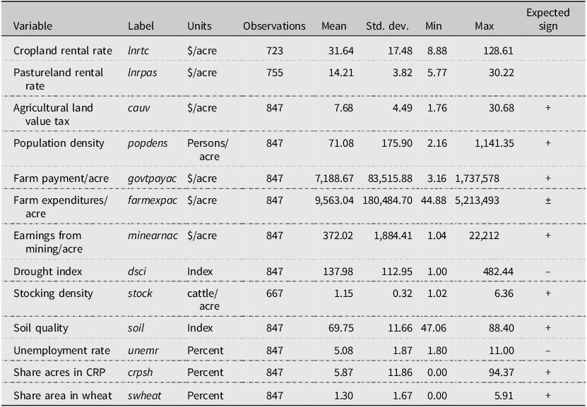
Annual county CAUV records are from the Oklahoma Tax Commission (Oklahoma Tax Commission, 2021). The CAUV variable is the total tax revenue collected from agricultural land divided by each county’s total farmland acres. Across all counties and years, the average CAUV was $7.68 per acre, ranging from $1.76 to $30.68 per acre (Table 1). Counties with the highest average CAUV were mainly metropolitan or neighboring metropolitan areas. Marshall County, the only other county with a relatively higher CAUV, is located on the state’s southern border across from the Dallas-Fort Worth metroplex. Oklahoma County experienced the most significant total change in CAUV from 2008 to 2019, with an increase of $48.86 per acre.
Summary statistics

Table 1 Long description
The table presents summary statistics for various agricultural and economic variables across counties. It includes data on cropland rental rate, pastureland rental rate, agricultural land value tax, population density, farm payments per acre, farm expenditures per acre, earnings from mining per acre, drought index, stocking density, soil quality, unemployment rate, share acres in CRP, and share area in wheat. The table has 13 rows and 9 columns, with each row representing a different variable and columns for label, units, observations, mean, standard deviation, minimum, maximum, and expected sign. Notable trends include high mean values for farm payments per acre and farm expenditures per acre, as well as significant variations in agricultural land value tax and population density.
Because the analysis is focused on land rental, we would ideally like to collect the CAUV for the rented land in the NASS cash rent surveys. Collection of this data was not possible, so we must assume that rented land is representative of all farmland in each county.
1.5. Additional independent variables
Control variables include agricultural and nonagricultural factors whose values influence equilibrium rental rates. Instead of solely shifting supply or demand, these covariates reflect how landowners and renters account for general market conditions, production costs, and regional contexts when determining equilibrium rents. Agricultural factors encompass program payments to farmers (govtpayac), CRP enrollment (crpsh), farm expenses (farmexpac), the county’s share of wheat production (swheat), the Drought Severity and Coverage Index (dsci), and soil productivity ratings (soil). Nonagricultural factors include population density (popdens), mining earnings (minearnac), and the unemployment rate (unemr) (Table 1). These variables serve as indicators of macroeconomic influences on rental rates, such as urban demand for land, the opportunity cost of renting agricultural land, and the opportunity cost of renting land.
Program payments to farmers and farm expenses are from the Bureau of Economic Analysis (BEA, 2021b). These payments apply only to acreage that produced eligible program crops: wheat, corn, sorghum, barley, oats, cotton, and soybeans. Therefore, the payments are calculated in dollars per acre of the respective crop. The land-use data for each category were obtained from Cropscape NASS (2021a) and extracted using CropscapeR (Chen, Reference Chen2020). Cropscape uses satellite imagery to estimate annual land coverage by category. Land use categories 1–60 were enumerated to determine total crop acreage, while category 176 includes all grassland and pasture acreage. Categories 1–5, 21–24, and 28 include program crops such as corn, cotton, rice, sorghum, soybeans, barley, wheat, and oats (Appendix Table A1). Payments to farms are expected to raise rental rates because these payments are capitalized into them (Alston, Reference Alston2010; Feng et al., Reference Feng, Hennessy and Miao2013; Hendricks et al., Reference Hendricks, Janzen and Dhuyvetter2012; Kirwan, Reference Kirwan2009).
Landowners with CRP acres receive annual payments for taking environmentally sensitive land out of production. CRP acres enrolled are reported by the USDA’s Farm Service Agency (USDA-FSA, Reference Agency2022). They are calculated as the proportion of the total acres enrolled in the CRP relative to the total farmable acres in a county. CRP acreage could influence the rental land market by decreasing the supply of rentable land. The CRP program generally limits enrollment to no more than 25% of a county’s eligible cropland.
Farm expenses are based on the BEA’s Farm Income and Expenses (BEA, 2021b). Expenses include seed, fertilizer, and lime in dollar amounts. Total expenses were calculated by dividing expenses by each county’s cropland acres. Farm expenses serve as a proxy for the production costs renters would face. Rental rates are expected to decrease as input costs rise.
Drought severity was measured using a DSCI, as explained by Akyuz (Reference Akyuz2017). The DSCI transforms categorical drought monitor data into a continuous scale by calculating a weighted sum of the percentage of each county affected by drought, where drought severity is categorized as D0 (abnormally dry), D1 (moderate drought), D2 (severe drought), D3 (extreme drought), and D4 (exceptional drought). The resulting scores range from 0, meaning no part of the county is experiencing drought, to 500, indicating the entire area is experiencing exceptional drought. Areas with less frequent drought conditions are likely to have higher rental rates because they are more attractive for agricultural production.
A soil rating variable was computed using the Natural Resources Conservation Service Web Soil Survey’s (Soil Survey Staff, Reference Staff2021) National Commodity Crop Productivity Index (NCCPI) using Dinterman and Katchova’s (Reference Dinterman and Katchova2020) method. The Web Soil Survey provides the total acreage of each soil type within each county. Each soil type is assigned an NCCPI rating based on its suitability for non-irrigated crop production. The Web Soil Survey provides NCCPI calculations for corn, soybeans, wheat, and cotton, as well as an overall NCCPI that records the highest rating among the four crop-specific ratings for each soil class. The overall NCCPI was assigned rather than using a crop-specific rating, assuming producers would grow the crops best suited to their soils. Since crop-specific ratings were not assigned based on specific crop acreage, variation among crop production composition from year to year is not a factor in the soil rating. The NCCPI reflects current conditions and does not account for actual land use. Profit-maximizing producers are assumed to select the most productive soils for crop production. The soil rating was calculated by allocating the total crop acres to soil types, starting with the soil with the highest productivity rating and moving to the next until all crop acres were distributed. The higher the land’s suitability for agriculture, the greater the demand for that land for farming purposes. The soil rating is likely to correspond with higher rental rates.
The area share of wheat acres planted in each county was included in the cropland rental rate model (swheat). Wheat is a major crop in Oklahoma. Counties that produce more wheat are expected to have higher cropland rental rates, as wheat production is a competitive use of land in the region. The wheat share variable was calculated by dividing the acres of wheat produced by the total acres of cropland in each county.
Nonagricultural factors believed to influence the rental rate are included as controls. Population density reflects urban pressures, as areas near metropolitan regions tend to be more densely populated than rural areas. Urban pressures serve as a proxy for land scarcity resulting from conversion to urban uses. Population density data from the United States Census Bureau (2021) are calculated as the total population divided by the county’s area in square miles.
We include the local unemployment rate to account for macroeconomic shocks that can influence cropland and pastureland rental rates through downstream effects, such as changes in off-farm earnings for farm households, local credit availability, and demand in agribusiness and competing land uses. In our model, unemployment acts as a broad indicator of the business cycle, helping to isolate the relationship between farm-sector variables and rental rates. The unemployment rate data is from the Bureau of Labor Statistics (2021).
Earnings from mining were included in the hedonic models because it is a significant economic sector in Oklahoma and competes with agriculture for land and labor. Oklahoma hosts a diverse range of mining activities, including oil, natural gas, coal, limestone, sand, gravel, gypsum, and other minerals (Pritchard, Reference Pritchard2022). Some mining operations can occur alongside farming, such as drilling for natural gas and oil. At the same time, other mining activities compete with farming due to their extraction processes. Therefore, if mining earnings increase, we would expect rental rates to rise to reflect the opportunity cost of land used for agriculture. Mining earnings data are from the BEA (2021a) and represent the opportunity cost of land use – comparing agricultural production to mining – for landowners and land renters. All prices are in 2016 dollars, calculated using the GDP deflator (BEA, 2021c).
1.6. Methods and procedures
Changes in one county’s tax policy can influence real estate prices in neighboring counties or municipalities through market linkages, labor mobility, or competitive dynamics (Cho et al., Reference Cho, Roberts and Lambert2016; Yang, Reference Yang2024). Taxes on agricultural land in nearby counties may also impact local rental rates (Yu and Rickman, Reference Yu and Rickman2012). Higher taxes in adjacent areas could make land in a specific county more attractive, affecting its rental prices. Counties might also engage in strategic actions, such as adjusting tax policies in response to neighboring jurisdictions (Genty et al., Reference Gentry, Greenhalgh-Stanley, Rohlin and Thompson2020; Luna, Reference Luna2004). These spillovers can create spatial externalities in local tax policies that directly influence economic outcomes, such as land values and rental rates (Burnett et al., Reference Burnett, Lacombe and Wallander2024, Reference Burnett, Lacombe and Wallander2025).
We estimate the hedonic models using two-way fixed effects (TWFE) spatial panel regression to analyze the potential spillover effects of changes in the CAUV on rental rates (Elhorst, Reference Elhorst and Elhorst2010). We use Hendry (Reference Hendry2024)’s general-to-specific identification procedure to select a plausible model that best captures spatial externalities. The initial model is the spatial Durbin (SDM), which nests the spatial autoregressive model (dependence in the response variable, known as the spatial autoregressive, or SAR model) and spatial error models (dependence in the errors, SEM) (LeSage and Pace, Reference LeSage and Pace2009). Under certain parameter restrictions, the SDM incorporates the SAR, TWFE, and SEM models.
We test these parametric restrictions by imposing common factor restrictions on the SDM first (Anselin et al., Reference Anselin, Serenini and Amaral2025). The SDM hedonic model is:
 $$ren{t_{it}} = \rho \cdot{{\bf{w}}_{j \ne i}}ren{t_{jt}} + {\alpha _1}\cdot cau{v_{it}} + {{\bf{x}}_{it}}{\bf{\beta}} \; + {{\boldsymbol\gamma }_{1}}\cdot{{\bf{w}}_{{j} \ne {i}}}{{\bf{cauv}}_{jt}} + {{\bf{w}}_{{j} \ne {i}}}{{\bf{x}}_{{jt}}}{\bf{\boldsymbol\gamma}}\; + {{u}_{{\it{it}}}}$$
where rent
it
is the natural log of the rental rate for location i and period t, cauv
it
are agricultural taxes lagged by one period (the variable of interest), and ${\bf x}_{it}$
includes the lagged control variables discussed above. The independent variables were lagged under the assumption that landowners base their rental rate decisions on expectations formed from a predetermined set of information. Lagged population density, government payments, farm expenses, mining earnings, stocking density, the CAUV, and rental rates are log-transformed, so the estimates represent elasticities.Footnote
1
${\bf x}_{it}$
includes the lagged control variables discussed above. The independent variables were lagged under the assumption that landowners base their rental rate decisions on expectations formed from a predetermined set of information. Lagged population density, government payments, farm expenses, mining earnings, stocking density, the CAUV, and rental rates are log-transformed, so the estimates represent elasticities.Footnote
1
The row vector ${\bf w}_{j\neq i}$
is from a 77 by 77 row-standardized queen contiguity matrix of the first order, with the unstandardized w
ii
elements equaling zero and w
ij
= 1 when county j neighbors i. Row-standardizing the contiguity matrix ensures that the model weights the influence of neighboring units by their relationship to the focal county, making spillover effects comparable across all counties (Anselin, Reference Anselin and Anselin2006). On average, five counties surrounded a typical county. We experiment with other definitions of spatial contiguity as a robustness check.
${\bf w}_{j\neq i}$
is from a 77 by 77 row-standardized queen contiguity matrix of the first order, with the unstandardized w
ii
elements equaling zero and w
ij
= 1 when county j neighbors i. Row-standardizing the contiguity matrix ensures that the model weights the influence of neighboring units by their relationship to the focal county, making spillover effects comparable across all counties (Anselin, Reference Anselin and Anselin2006). On average, five counties surrounded a typical county. We experiment with other definitions of spatial contiguity as a robustness check.
The variable u it = μ i + τ t +v it is a composite error, with the μ i county fixed effects, τ t yearly fixed effects, and v it a random error term with an expected value of zero and a potentially nonconstant variance. We parametrize the county- and year-fixed effects using an orthogonal transformation proposed by Lee and Yu (Reference Lee and Yu2010). Lee and Yu show that the traditional FE transformation creates linear dependencies in the model disturbances when the spatial weights matrix is constant over time. These linearities impact the consistency of the parameter estimates and their variances. After demeaning, any remaining cross-unit correlation should primarily reflect spatial dependence through W or contemporaneous common shocks in v it . A disadvantage of this transformation is that it requires removing a panel from the dataset.
We estimate the panel SDM using maximum likelihood with the xsmle Stata procedure (StataCorp, 2023), as developed by Belotti et al. (Reference Belotti, Hughes and Mortari2017).Footnote 2 We use the maximum likelihood estimates to select the most plausible model by testing parametric restrictions. The SDM reduces to the TWFE, cross-regressive (SLX, Florax and Folmer, Reference Florax and Folmer1992), SAR, or SEM models under the following null hypotheses (Anselin, Reference Anselin and Anselin2006; LeSage and Pace, Reference LeSage and Pace2009):
-
A. H0-TWFE: $\rho = {\gamma _1} = {\bf{\gamma}} \; = {\bf{0}}$
,
$\rho = {\gamma _1} = {\bf{\gamma}} \; = {\bf{0}}$
, -
B. H0-SLX: ρ = 0,
-
C. H0-SAR:
${\gamma _1} = {\bf{\gamma}} \; = {\bf{0}}$
, -
D. H0-SEM: γ k + ρ ⋅ β k = 0 for all k covariates.


Anselin et al. (Reference Anselin, Serenini and Amaral2025) outline the steps to derive these relationships under the common-factor specification of the SDM and the general-to-specific approach for identifying spatial models. A Wald statistic is calculated to test each hypothesis. A cluster-robust covariance matrix (Liang and Zeger, Reference Liang and Zeger1986) is used to compute the Wald statistic and the standard errors of the model estimates, with clustering on the counties. Clustering on counties allows for arbitrary serial correlation of the residuals within counties, with standard errors robust to heteroskedasticity (Cameron and Miller, Reference Cameron and Miller2015).
We report the direct and indirect effects of the CAUV on rental rates using the SDM or SAR model estimates (Elhorst, Reference Elhorst2014). The county direct effect elasticities for the SDM, α̂ 1i D , are the diagonal elements of the 77 by 77 matrix,
 $${\partial \ln \boldsymbol{rent} \over \partial \ln \boldsymbol{cauv}}=\left({\bf I}_{N}-\hat{\rho }{\bf W}_{N}\right)^{-1}\left({\bf I}_{N}\hat{\alpha }_{1}+{\bf W}_{N}\hat{\gamma }_{1}\right)$$
(LeSage and Pace, Reference LeSage and Pace2009). The indirect effect elasticities are the impact of a change in county i’s CAUV on the rental rate in county j. The indirect effect elasticities, α̂
1i
I
, are calculated as the row-sums of the same 77 by 77 matrix. The SAR direct and indirect effect elasticities are the same expression, but exclude ${\bf W}_{N}\hat{\gamma }_{1}$
. The county-level direct and indirect effect averages of the elasticities are reported in the regression output. The delta method (Greene, Reference Greene2018) is used to calculate the standard errors of these effects using a cluster-robust covariance matrix.
${\bf W}_{N}\hat{\gamma }_{1}$
. The county-level direct and indirect effect averages of the elasticities are reported in the regression output. The delta method (Greene, Reference Greene2018) is used to calculate the standard errors of these effects using a cluster-robust covariance matrix.
1.7. Incidence calculations
We aim to investigate the impact of a $1 change in the CAUV on cropland and pasture rental rates, specifically examining its incidence. We use the elasticity identity to estimate the county-specific direct or induced effects of the incidence as
 $${\widehat{\partial rent}_{i} \over \partial cauv_{i}}=\hat{\alpha }_{i}^{D}\cdot {\overline{\widehat{rent}}_{i} \over \overline{cauv}_{i}}\ {\rm or}\ \hat{\alpha }_{i}^{I}\cdot {\overline{\widehat{rent}}_{i} \over \overline{cauv}_{i}},$$
where $\overline{\widehat{rent}}_{i}$
is the county-time average of the predicted county rental rate from a regressionFootnote
3
and
$\overline{\widehat{rent}}_{i}$
is the county-time average of the predicted county rental rate from a regressionFootnote
3
and $\overline{cauv}_{i}$
is the county-time average of the CAUV. For the SEM and TWFE models, the spatially varying effects of the CAUV on the rental rate are replaced by α̂
1.
$\overline{cauv}_{i}$
is the county-time average of the CAUV. For the SEM and TWFE models, the spatially varying effects of the CAUV on the rental rate are replaced by α̂
1.
We estimate the incidence for each county by averaging the changes in the tax rate over the years. We then use these averages to analyze the spatial distribution of both direct and indirect effects of the incidence on rental rates. The county incidences also help us estimate the total monetary amount passed on to cropland and pastureland renters due to the CAUV. Changes in the tax rate for each year are aggregated for each county in the study region, yielding the total tax change over the study period for each county. This total change is then multiplied by the county-specific incidence. The incidence for each county is further multiplied by the number of acres of rend cropland and pastureland. All county incidences are summed to yield the total incidence incurred by renters over the period. Since the exact number of acres rented is unknown, we assume the state follows the national average: 54% of cropland and 28% of pastureland are rented (Bigelow, Reference Bigelow2016) when calculating the total incidence. Oklahoma has a total rented percentage of 41%, which is almost the same as the 39% reported by Bigelow et al. (2016) for cropland- and pasture-specific percentages. This correspondence gives us confidence in our use of national cropland and pasture percentages.
1.8. Multiple imputation and SDM estimation
The objectives of regression analysis with missing data are to reduce bias caused by missing values, maximize the utilization of available information in the dataset and model structure during imputation, and produce estimates of parameter uncertainty. We use a model-based multiple-imputation (MI) procedure with chained equations (MICE) to fill in missing values for pastureland and stocking density. MICE is a flexible and widely used approach that iteratively models each variable with missing data as a function of other variables in the dataset (White et al., Reference White, Royston and Wood2011).
One MICE imputation method is predictive mean matching (PMM) (van Buuren, Reference Stef2012). PMM is a semi-parametric procedure that ensures imputed values come from observed data, helping to maintain the original distribution and avoid unrealistic values. Missing values are replaced with observed values from a donor observation that has similar predicted outcomes based on a regression model. The locations of missing values were imputed using PMM with the five nearest neighbors, which is the average number of neighbors identified by the spatial weighting matrix.
The function used to simultaneously PMM-impute missing pastureland rental rates and stocking densities is a modified version of Equation. 1. Namely,
 $$\left[ {\matrix{ {pastrent_{it}} \cr {stock_{it}} \cr {croprent_{it}} \cr } } \right] = \left[ {\matrix{ {{\rm{linear}}({stock_{it}},{croprent_{it},cauv_{it}},{\bf{x}}_{it},{\bf{W}}cauv_{it},{\bf{Wx}}_{it},\;{\mu_{i}},{\tau_{t}})} \cr {{\rm{linear}}(pastrent_{it},croprent_{it},cauv_{it},{\bf{x}}_{it},{\bf{W}}cauv_{it},{\bf{Wx}}_{it},\;{\mu_{i}},{\tau_t})} \cr {{\rm{linear}}(stock_{it},pastrent_{it},cauv_{it},{\bf{x}}_{it},{\bf{W}}cauv_{it},{\bf{W}}{{\bf{x}}_{it}},\;{\mu_i},{\tau_t})} \cr } } \right]$$
where the right-hand side variables are observed. MICE employs an iterative Monte Carlo procedure to generate posterior distributions of the PMM-imputed missing variables. We adopt a burn-in value of 1000 and a thinning value of 100 between Monte Carlo draws. Additionally, we bootstrap imputed values from the corresponding posterior distributions, as we remain agnostic about the underlying data-generating process of the missingness. Stata’s mi impute chained procedure (StataCorp, 2023) was utilized to implement the MICE-PMM procedure for missing pastureland and cropland rental rates and stocking density. We produce 70 imputed data sets. Each data set replicates the original, maintaining its complete entries and including imputed values for missing variables.
One approach to address MNAR in an implementation procedure is to include external information that causes MNAR (White et al., Reference White, Royston and Wood2011). The number of farms per acre of cropland and pastureland was used as external information and entered into the imputation algorithm as importance weights. Farm density is used as a proxy for the non-disclosure policy that suppresses rental rates when farms can be identified in a county. The agricultural census provides county-level estimates of farm numbers every five years. We interpolated the farm numbers per county in inter-census years using a procedure that estimates county/farm numbers by proportionally downscaling the total number of farms in Oklahoma, which is never suppressed, to counties (Appendix A2).
Regression with imputed data requires running multiple regressions on the MI data sets. The estimated parameters from each regression are collected and then averaged. A covariance matrix is calculated for these estimates for inference. We use the fraction of missing values (FMI) statistic to determine the number of regressions required to achieve a reliable covariance estimator for convergence (Schaefer and Grahm, Reference Schafer and Graham2002). The FMI is calculated as [V̂
B
+V̂
B
/M]/V̂
W
, where V̂
B
measures the variability in the parameter estimates obtained from M imputed datasets and V̂
W
is the mean of the sampling variances from each of the M imputed datasets. Determining an optimal M is important for estimating the total variance of the M imputed vectors of parameter estimates, ${V_T}(\overline {\theta \;} )$
, which is the total covariance. Rubin’s (Reference Rubin1987) approximation of the imputed total covariance is:
${V_T}(\overline {\theta \;} )$
, which is the total covariance. Rubin’s (Reference Rubin1987) approximation of the imputed total covariance is:
 $${V_T}\left( {\overline \theta } \right) = {1 \over M}\sum\nolimits_{m = 1}^M V \left( {{{\widehat{\theta }}_m}} \right) + {{M + 1} \over {M\left( {M - 1} \right)}}\sum\nolimits_{m = 1}^M {\left( {{{\widehat{\theta}}_m} - \overline {\theta \;} } \right)} \left( {{{\widehat\theta }_m} - \overline {\theta \;} } \right)',$$
where the first term on the right-hand side of the equality is V̂
W
, the second term V̂
B
, the $\hat{\bf \theta}_{m}$
vectors of regression estimates estimated with data set m, and
$\hat{\bf \theta}_{m}$
vectors of regression estimates estimated with data set m, and $\overline{\bf \theta\ }$
the averages of the M vectors of estimates. We use the cluster-robust covariance estimator for the
$\overline{\bf \theta\ }$
the averages of the M vectors of estimates. We use the cluster-robust covariance estimator for the $V(\hat{\bf \theta}_{m})$
(Liang and Zeger, Reference Liang and Zeger1986). White et al. (Reference White, Royston and Wood2011) suggest determining the number of regressions on MI data as #Regressions ≥ 100 × FMI. The TWFE and spatial regressions are estimated M times according to this rule.
$V(\hat{\bf \theta}_{m})$
(Liang and Zeger, Reference Liang and Zeger1986). White et al. (Reference White, Royston and Wood2011) suggest determining the number of regressions on MI data as #Regressions ≥ 100 × FMI. The TWFE and spatial regressions are estimated M times according to this rule.
2. Results and discussion
2.1. Cropland rental rate
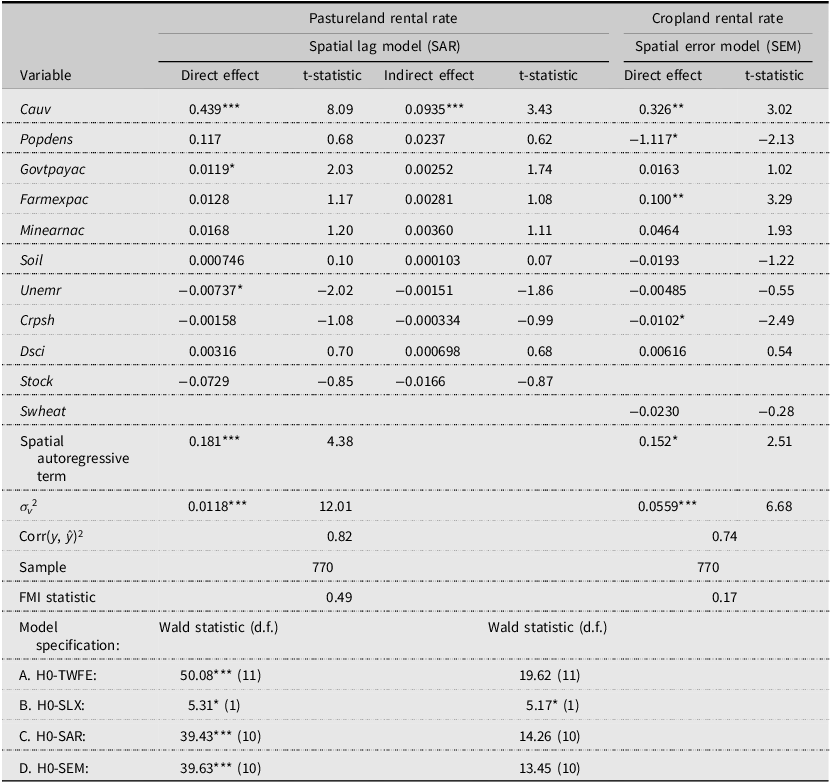
The results of hypotheses A, B, C, and D are shown in Table 2. Appendix Tables A3 and A4 provide all the model estimates, including the aspatial TWFE results.Footnote 4 The null hypotheses could not be rejected in any case. The failure to reject the null hypothesis in D suggests that the preferred spatial model exhibits autocorrelated errors (SEM). The FMI statistic was 0.17, leading us to use 17 of the 70 imputed data sets to estimate the SEM model 17 times. The squared correlation between the observed and predicted rental rates, 0.74, indicates that the SAR model fits the data reasonably well. The autoregressive estimate is 0.15 (t-statistic = 2.51, p < 0.05), indicating that the error terms of the cropland hedonic model are positively spatially correlated.
Pasture and cropland rental rate regressions

Table 2 Long description
The table presents a comparison of pastureland and cropland rental rates using spatial lag (SAR) and spatial error (SEM) models. It includes direct and indirect effects of various variables, along with their t-statistics. The variables include Cauv, Popdens, Govtpayac, Farmexpac, Minearnac, Soil, Unemr, Crpsh, Dsci, Stock, and Swheat. The table also shows spatial autoregressive terms and model statistics such as sigma squared, correlation between observed and predicted values, sample size, and FMI statistic. The model specifications include Wald statistics for different hypotheses.
Notes: *p < 0.05, **p < 0.01, ***p < 0.001.
We report the direct effects of the SEM model that are significant at the 5-percent level or lower. The CAUV had a significant effect of 0.33 on cropland rental rates, indicating that for every 1% increase in the CAUV, cropland rental rates rose by 0.33%. After transforming this number, a $1 increase in the CAUV translates to an average increase of $0.08 in the cropland rental rate. An increase in the CAUV was expected to lead to higher rental rates, as landowners share the increased tax burden with the renters. These results for rented cropland are smaller in magnitude than those of Dinterman and Katchova (Reference Dinterman and Katchova2020), who found that rental rates increased by $0.31 to $0.61 per additional tax dollar in Ohio. Oklahoma’s lower cropland incidence is likely due to its comparatively lower soil productivity compared to Ohio’s.
When the effect of the CAUV was calculated for each county, incidence estimates ranged from less than a cent per dollar of tax in Cimarron County to $0.48 per dollar of tax in Marshall County. These results are not surprising. When the CAUV map (Figure 1) is compared to the Cropland Incidence map (Figure 2), the counties with the highest incidences are those with relatively high CAUV and relatively low cropland rental rates. As discussed earlier, Marshall County is located north of the Dallas-Fort Worth metro area and has plentiful access to water, both of which increase the competition for land in that region. Similarly, Creek County and McIntosh County, situated near the Tulsa Metropolitan area, had comparatively high incidences of $0.27 and $0.19. The combination of high CAUV with low rental rates naturally leads to a greater portion of the tax burden being passed on to renters. These county incidences were used to estimate a total cropland rental incidence of $101,680 over the study period and all counties, assuming that the amount of cropland rented followed the national average of 54% (Bigelow et al., Reference Bigelow2016).
County-level map of current agricultural use value, cropland rental rates, and pastureland rental rates.

Figure 1 Long description
A heat map displays the current agricultural use value, cropland rental rates, and pastureland rental rates across counties in the United States. The map is divided into three sections: Current Agricultural Use Value (CAUV), Cropland Rental Rates, and Pastureland Rental Rates. Each section uses a color gradient to represent different values. The CAUV section ranges from 5 to 20 dollars per acre, with darker colors indicating higher values. The Cropland Rental Rates section ranges from 20 to 60 dollars per acre, and the Pastureland Rental Rates section ranges from 7.5 to 15 dollars per acre. The map shows variations in agricultural use value and rental rates across different counties, with some regions showing higher values and others lower values.
County level CAUV elasticities and incidences for cropland and pastureland.

Figure 2 Long description
The image contains four maps of the United States, each representing different data related to cropland and pastureland. The top left map shows cropland CAUV elasticity, with varying shades indicating percentage changes across counties. The top right map displays pasture CAUV elasticity, similarly using color gradients to represent percentage variations. The bottom left map illustrates cropland incidence, with colors indicating dollar per acre values. The bottom right map shows pasture incidence, also using a color scale to depict dollar per acre values. Each map uses a color gradient from blue to yellow to represent different ranges of values, with blue indicating lower values and yellow indicating higher values. The maps provide a visual representation of how CAUV elasticities and incidences vary across different counties in the United States.
Population density negatively affected cropland rental rates. The result was unexpected. The negative relationship might be attributable to agricultural parcel fragmentation around urban areas (Wadduwage et al., Reference Wadduwage, Millington, Crossman and Sandhu2017). Fragmented agricultural land may limit production options and the economies of scale that come from farming larger, intact parcels, resulting in lower demand for fragmented farmland parcels and, consequently, lower rental rates. This assumption is supported by Lu et al. (Reference Lu, Xie, He, Wu and Zhang2018), who found that land fragmentation negatively affected agricultural land value due to changes in yield and the high opportunity cost of labor.
Farming expenses had a significant positive effect on rental rates. Farm management analysts anecdotally recognize that rental rates increase with farm input costs, which rise in response to rising commodity prices (Laporte et al., Reference Laporte, MacKellar and Pennington2023; Thiesse, Reference Thiesse2023). These observations are supported by the findings of Lippman and Rumelt (Reference Lippman and Rumelt2003), who reported that increases in input costs correlated with higher land rents until the point where that land would be more profitable if switched to another land use.
CRP had a significant negative effect on cropland rental rates. This outcome was unexpected. Increased CRP enrollment was expected to raise rental rates due to decreased availability of rentable land. Lower CRP enrollment might lead to higher rental rates because landowners receive less income from CRP. Moreover, by definition, CRP acres are low-quality land.
2.2. Pastureland rental rate
The results for hypotheses A, B, C, and D are in Table 2. The null hypotheses were rejected in each case, indicating that the SAR model best characterized the spatial interaction between counties and the CAUV levels they establish. The FMI statistic was 0.49, leading us to use 49 of the 70 imputed data sets to estimate the SAR model 49 times. The squared correlation between the observed and predicted rental rates (0.83) indicates that the SAR model fits the data well. The estimate for the autoregressive term is 0.18 (t-statistic = 12.01, p < 0.001), indicating positive spatial feedback in county rental rates. We report the direct and indirect effects of the SAR estimates. The total effects (direct + indirect) are reported in Appendix Tables A3 and A4.
The CAUV had a significant direct effect of 0.44 on pastureland rental rates, indicating that a 1% increase in the CAUV was associated with a 0.44% increase in rent within the same county. Converted to dollars, a $1 increase in the CAUV led to an average increase of $0.40 in pastureland rents per acre. Pastureland incidences have not been studied previously, but this incidence is comparable to the cropland incidence found by Dinterman and Katchova (Reference Dinterman and Katchova2020) of $0.31 to $0.61 per additional tax dollar. Pastureland is a competitive land use in Oklahoma, as reflected by the incidence.
When estimating the effects of the CAUV at the county level, the findings closely resemble the spatial distribution of cropland incidences, but are relatively higher. The incidences ranged from a low of $0.10 in Cimarron County to a high of $3.37 in Marshall County. The highest incidences were mainly in counties with comparatively high tax rates and low rental rates. The counties with the highest incidences were Marshall, Oklahoma, Creek, and Cleveland Counties, at $3.37, $3.01, $1.94, and $1.56, respectively. Notably, 10 of the 77 counties in Oklahoma had incidences over $1, indicating that rents increased by more than a dollar for each additional dollar taxed (Marshall, Oklahoma, Creek, Cleveland, Wagoner, Carter, Washington, Pottawatomie, Rogers, and McIntosh). This finding suggests that not only was a substantial portion of the tax burden shifted to renters in these counties, but the demand for this land was strong enough for landowners to charge more than the tax amount to renters. The total pastureland for the state was estimated from the county incidence data, assuming that 28% of each county’s pastureland was rented. The result suggests an estimated incidence of $7,726,319 over the study period and all counties. This number is likely a conservative estimate, as Oklahoma is projected to have a higher acreage of rented pastureland compared to the national average.
Program payments had a positive, significant effect on pastureland rental rates. This outcome was expected, as there is evidence of landowners capturing government payments through increased rental rates (Alston, Reference Alston2010; Alston and James, Reference Alston and James2002; Hendricks et al., Reference Hendricks, Janzen and Dhuyvetter2012; Katchova and Ahearn, Reference Katchova and Ahearn2015; Kauffman, Reference Kauffman2013; Kirwan, Reference Kirwan2009).
The unemployment rate had a negative relationship with pastureland rents. This finding was anticipated. Many individuals who rent farmland have off-farm work opportunities. If off-farm income cannot fill the gap in farm-rented land income, those operators may struggle to continue renting land. The decline in demand for rented land consequently reduces rents.
In addition to the direct effects, the SAR model also captures indirect effects. The only significant indirect effect was the CAUV, with a value of 0.09. The interpretation of this coefficient is that an increase in CAUV in one county leads to higher rental rates in neighboring counties. This externality is not surprising, as we would expect to see spillover effects of land use tax policies into adjacent counties with a similar context. Land formations, land quality, and land use are generally more similar within neighboring counties than across the state. Additionally, individuals who own land in a region may own parcels in nearby counties. All of these factors could contribute to higher rental rates in counties adjacent to those where the CAUV increased.
3. Conclusions
This study examined how agricultural land taxes are passed on to cropland and pastureland renters as a tax incidence in Oklahoma. The findings show that both land types exhibit positive tax incidence. On average, a one-dollar increase in the current agricultural use value (CAUV) tax corresponded to a $0.08 increase in cropland rents and a $0.40 increase in pastureland rents per acre. Aggregated across the study period, pastureland renters absorbed an estimated $7.73 million in additional costs, equivalent to about 22 percent of the total tax revenue. The effect was smaller for cropland rental rates, with an estimated additional cost of $101,680. These results indicate that a portion of the agricultural tax burden is shifted from landowners to renters, with stronger pass-through to pastureland renters.
Pastureland rental rates are more responsive to land tax policies than cropland rental rates. Although the incidence of property taxes on pastureland has grown more rapidly than for cropland, rental rates have not kept pace, implying that landowners absorb much of the tax burden rather than fully passing it on to tenants. Some of the tax burden relief likely occurs through modest rent adjustments rather than large-scale land conversion. The high incidence in counties adjacent to metropolitan areas suggests that proximity to urban markets intensifies competition for land and amplifies tax incidence effects.
These results have several practical implications. Since property tax assessments in Oklahoma are determined locally, adjusting the assessment formula could help better align tax burdens with local land-use conditions and fiscal policy. Counties with a comparatively high incidence of pastureland may consider differential assessment percentages to moderate renter exposure. However, programs that offset land taxes through subsidies risk being capitalized into rents and captured mainly by landowners, as prior research demonstrates. Any local tax adjustments should therefore be evaluated alongside their distributional effects within the crop and pastureland rental markets.
Finally, the analysis underscores that observed incidences arise from equilibrium market responses, not necessarily from inefficiencies. Policies aimed at equalizing tax burdens should account for regional variation in crop and pastureland markets and the interactions between agricultural and nonagricultural land uses. Future work could extend this analysis to other states, examine parcel-level data where available, and incorporate nonagricultural uses of pastureland, such as hunting leases, to improve understanding of how land taxation affects different segments of the agricultural rental market.
Supplementary material
The supplementary material for this article can be found at https://doi.org/10.1017/aae.2025.10034.
Data availability statement
The data were obtained from publicly available sources and through a special request from the Oklahoma Tax Assessors’ Office. There are no data restrictions.
Acknowledgements
This research was supported by the USDA Hatch Multistate Project NE-2249 OKL03125 and the Willard Sparks Chair in Agricultural Sciences & Natural Resources, Oklahoma State University Division of Agricultural Sciences and Natural Resources. The authors appreciate the comments and suggestions of three anonymous reviewers, which substantially improved the manuscript.
Author contribution
Conceptualization, D.M.L.; Methodology, D.M.L.; Formal Analysis, K.W. and D.M.L.; Data Curation, N.H.L.; Writing – Original Draft, K.W., Writing – Review and Editing, K.W., D.M.L., N.H.L.; Supervision, D.M.L.; Funding Acquisition, D.M.L.
Financial support
This research was funded by the Willard Sparks Chair in Agricultural Sciences and Natural Resources, Oklahoma State University Division of Agricultural Sciences and Natural Resources, and USDA Hatch Multistate Project NE-2249 OKL03125.
Competing interests
Welch, Lansford, and Lambert declare none.


 Open access