
Water-quality trading is a mechanism that can improve the economic and environmental performance of measures designed to control water pollution. The case for trading is that markets can allocate emissions of pollution from various sources more efficiently than traditional regulatory instruments and allow regulators to achieve pollution targets with less information (Horan and Shortle Reference Horan and Shortle2011). However, water-quality trading also poses a number of challenges related to the design of markets that can achieve their theoretical potential (Fisher-Vanden and Olmstead Reference Fisher-Vanden and Olmstead2013, Horan and Shortle Reference Horan and Shortle2011, Shortle Reference Shortle2013). One of those challenges is lag time inherent to water systems between efforts to alleviate or remediate pollution and changes in the quality of the water.
Following textbook models of pollution trading, water-quality markets are typically designed under the assumption that improvement in the ambient environmental water quality achieved by pollution-abatement efforts is fully realized during the period in which abatement is being implemented. Thus, point sources of water pollution have been allowed, under water-quality trading programs, to immediately substitute credits from implementation of agricultural best management practices (BMPs) for reductions in point-source effluent based on the general premise that the pollution reductions are immediate. This assumption greatly simplifies market design but does not validly represent the often-slow response of ambient water quality to reductions in nonpoint pollution.
Markets designed under the assumption of contemporaneous substitution can adequately perform the economic functions of a market (economic efficiency) but will fail to achieve their ecological functions (reducing pollution to achieve water-quality goals) for some period of time related to the length and structure of any lags present. The market “fix,” in theory, is to allow for trading across potentially lengthy periods and across space. But futures markets for trading commodities over long periods are extremely complex to implement, are expensive to operate, and do not necessarily perform well economically when the commodity is complex (as is the case with water quality) and/or there is significant uncertainty about economic conditions and regulatory environments in the future (Carlton Reference Carlton1984). Consequently, it can be useful to rely on the simplicity of markets designed under the assumption of contemporaneous substitution (i.e., no lags) if the smaller cost associated with the simpler design is significant and the delay in achieving the environmental targets is acceptable.
This research is motivated by a need to understand the implications of lags in the ambient level of agricultural pollution in waterbodies for the efficiency and design of water-quality markets. We are especially interested in comparing simple market designs based on the assumption of contemporaneous substitution with complex dynamic market designs that facilitate trading across time and space. For this analysis, we compare the outcomes of pollution-control efforts under simple and complex dynamic allocation rules in the context of nutrient pollution in Chesapeake Bay and identify conditions under which the simple allocation rules perform well. We begin with a conceptual model of efficient pollution-control allocations with lags to develop key concepts and the analytical framework used for this study. We then apply the models to control of nitrogen pollution in Chesapeake Bay.
A Model of Efficient Pollution Control with Lags
Market-based approaches to pollution control entail direct or indirect exchanges of property rights related to emitting pollution. Fundamental tasks in the design of such markets are (i) defining the tradable commodity to which the property rights apply, (ii) specifying trading rules governing exchanges of the commodity, and (iii) specifying aggregation rules to limit the aggregate supply of the commodity so that the market's allocations of pollution emissions do not violate the overarching environmental goal of the trading program (Horan and Shortle Reference Horan and Shortle2011). Lags in the effect of pollution-control efforts have implications for each of these tasks.
In a simple “textbook” model of pollution-permit trading without lags, the amount of pollution (the load) that reaches and is measured at receptor locations (e.g., the mouth of the Susquehanna River on Chesapeake Bay) during the year depends entirely on emissions into the water during that period, and substitution credits are calculated for each source based on those loads and the appropriate trading ratio. With lags, pollutants emitted in one year may reach the receptor during that year or in subsequent years. If the policy goal is to limit pollution reaching the receptor in a given year to a specific amount, the definition of the commodity and the trading and aggregation rules must account for the lagged delivery of pollution.
To introduce lags, we begin by indexing emissions not only by source but also by the year released. Emissions from source i at time t are represented by e it , and some fraction of a source's emissions reach a regulated waterbody and contribute to ambient pollution at a receptor at a future time. For simplicity, we assume that the future delivered fraction is not distributed over a period of time and instead arrives on a specific date, t + l. The amount delivered at that time from source i is given by θ il · e it (0 ≤ θil ≤ 1) where l is the lag time between emission and delivery at the receptor and θ il is the fraction of the emissions that reach the waterbody. This fraction, referred to here as a delivery factor, is generally less than one for nutrients since nutrients are removed from water by various processes as the water flows through tributaries from source to the receptor. Each source has a fixed lag time, but the lag times can vary from source to source.
Let t = 0 be the date at which a new management strategy is implemented. At that date, the waterbody already contains a base load, B t , that consists of a sequence of legacy pollutant loads from prior point and nonpoint emissions plus pollution from unmanaged natural sources. The legacy component of the base load generally decays over time as the pollutants work their way down the watershed. Thus, over time, B t converges to the natural background load associated with natural events (including whatever lags exist in that process). The pollution reaching the receptor at any time t ≥ 0 is the legacy load plus the load generated since implementation of the new management strategy:
 $$L_t = B_t + \sum\nolimits_{k = 0}^t \sum\nolimits_{i = 1}^{m_k} \theta _{il}e_{ik}$$
where m k is the number of sources discharging at time k(0 ≤ k ≤ t). For simplicity, this number is fixed (equal to m). The second term on the righthand side of equation 1 is the manageable component of the pollution at period t = 0. This component is composed of emissions between the start of the management period and time t. Emissions at any time k < t with a lag of greater than t – k will appear in the delivered load subsequent to time t.Footnote 1
Environmental policymakers impose a limit, L t max , on the amount of pollution reaching the regulated receiving water for each time t in the planning horizon. Thus, in each period t, they require that
 $$B_t + \sum\nolimits_{k = 0}^t \sum\nolimits_{i = 1}^m \theta _{il}e_{ik} \le L_t^{max}.$$
A minimal requirement for the goal to be feasible is that B t ≤ L t max . The difference between the goal and base load is the allowable level of the managed load.
When lags are incorporated, the cost of achieving the pollution target for a particular period is realized over multiple periods. Consequently, efficient pollution control plans require allocation of the reductions in emissions over both time and space to minimize the present value of the cost of achieving the goal. In the model, the abatement cost for source i at time t is denoted as c i (e it ). This function is taken to be continuous, convex, and decreasing in emissions (i.e., more pollution, less pollution abatement, less cost). The present value of the societal cost of pollution control from all sources beginning at t = 0 and extending over time horizon T is then given by
 $$ \sum\nolimits_{t = 0}^T \sum\nolimits_{i = 1}^m c_i\lpar {e_{it}} \rpar\beta _t$$
where β t = (1 + r)–t and r is the discount rate. The Lagrange equation for the optimization problem is
 $$J = \sum\nolimits_{t = 0}^T \sum\nolimits_{i = 1}^m c_i\lpar {e_{it}} \rpar\beta _t + \sum\nolimits_{t = 0}^T \rho _t[{L_t^{max} - \; B_t - \sum\nolimits_{k = 0}^t \sum\nolimits_{i = 1}^m \theta _{il}e_{ik}}]$$
where ρt is the Lagrange multiplier for the environmental constraint at time t. When assuming an interior solution,Footnote 2 the first-order necessary conditions for the optimization problem are
 $$\displaystyle{{\partial J} \over {\partial e_{it}}} = \displaystyle{{\partial c_i} \over {\partial e_{it}}}\beta _t - \rho _{t + l}\theta _{il} = 0.$$
Emissions at time t for any source with lag l substitute for emissions from all other sources that reach the regulated waterbody in period t + l and may have occurred in periods prior to t for sources with lag lengths greater than l or in periods subsequent to t for sources with lag lengths less than l. Accordingly, for any source j discharging at time t + k ≤ t + l (–t ≤ k ≤ l) for which emissions also arrive at time t + l, equation 5 implies that an optimal allocation requires that
 $$\displaystyle{{\partial c_i} \over {\partial e_{it}}}\displaystyle{1 \over {\theta _{il}}} = \; \displaystyle{{\partial c_j} \over {\partial e_{\,j\lpar {t + k} \rpar}}}\displaystyle{{\beta _k} \over {\theta _{\,j\lpar {l - k} \rpar}}}.$$
The lefthand side of equation 6 is the marginal cost of reducing source i's emissions at time t divided by the proportion of the emissions that reaches the receiving water l periods later. With this division, the term can be interpreted as the marginal cost of reducing the source's contribution to ambient pollution at time t + l. The marginal gain of a decrease in ambient pollution by source i at time t + l due to the reduction in emissions at time t is the foregone cost of reducing pollution from other contributing sources of pollution at time t + l to satisfy the ambient pollution constraint at that time.Footnote 3 This foregone cost is given by the righthand side of equation 6 for source j discharging pollution at time t + k and reaching the receiving waterbody at time t + l. Condition 6 indicates that, in optimality, the marginal cost of abatement for source i at time t is equal to the discounted marginal abatement cost for source j at time t + k.Footnote 4
The system modeled in equation 6 has important implications for pollution management. Inequalities in marginal abatement costs are often used as indicators of inefficiency in pollution control policies, and in simple static models, those inequalities imply that cost savings can be realized by reallocating abatement from sources with high marginal abatement cost to sources with lower marginal abatement cost. For example, the observation that the marginal costs of agricultural nonpoint-source (NPS) abatement are often lower than the marginal costs of point-source (PS) abatement is used as an indication that the allocation of NPS and PS emissions is inefficient and to conclude, therefore, that there are potential gains from pollution trading. However, equation 6 implies that the marginal abatement costs for lagged sources are less than those for non-lagged sources in the dynamically efficient allocation with lags. Thus, a difference in marginal abatement cost does not necessarily imply an inefficient allocation and potential gains from trading. In addition, the equation indicates that differences in the marginal abatement cost in an efficient solution will vary with lag length and the discount rate. The differences will be greatest when comparing a non-lag source to a lagged source and will increase with the lag length and the discount rate.
A natural form of a market that trades pollutants with lagged delivery is one in which polluters can buy and sell forward. For example, BMPs implemented today will not have an impact on emissions until sometime in the future so the farmer could contract in advance to sell those future credits to a point source polluter. In theory, a perfectly competitive futures market could achieve a dynamically efficient allocation. However, forward markets that involve long periods can be expensive to set up and operate, as well as complex for participants (e.g., Carlton Reference Carlton1984). We do not attempt to estimate those set-up and operating costs, but it only makes sense to incur them if the resulting allocation achieves significantly better results than a static market design.
We ask whether the results of the simpler, less costly static market design can be reasonably comparable to the results of the complex and costly dynamically efficient allocation. In other words, do we need to account for lags when designing pollution-abatement markets? We explore this question using a model of control of nitrogen pollution from PSs and agricultural pollution from NPSs in Chesapeake Bay as a case study.
Lags and Efficient Load Allocations for Chesapeake Bay
Reducing nutrient and sediment pollution in Chesapeake Bay has been a major policy goal of the U.S. Environmental Protection Agency (EPA) and the states in the bay's watershed since the early 1980s. Limited progress led EPA to issue a total maximum daily load (TMDL) for the bay in December 2010. The TMDL specifies limits on the loads of applicable NPS emissions and waste loads of applicable PS emissions that must be achieved by 2025 for nitrogen, phosphorus, and sediment by all polluting sectors (agricultural operations, wastewater treatment plants, run-off from regulated and unregulated urban and suburban areas, septic systems, forests, and air deposits) collectively (Kaufman et al. Reference Kaufman, Abler, Shortle, Harper, Hamlett and Feather2014). The limits apply to jurisdictions in the portions of the states (Delaware, Maryland, New York, Pennsylvania, Virginia, and West Virginia) that fall within the watershed and the District of Columbia. We omit the District of Columbia because it contains no agricultural land.
The TMDL and waste load limits take the relative effectiveness of measures to reduce pollution in the bay, the relative contribution of each source and location, and other factors into account. They do not, however, explicitly take the relative cost-effectiveness of those sources and locations into account. Furthermore, the watershed implementation plans (WIPs) that describe practices the states plan to implement to meet the TMDL limits are not developed to be cost-minimizing (Kaufman et al. Reference Kaufman, Abler, Shortle, Harper, Hamlett and Feather2014). This lack of attention to cost-effectiveness suggests that there is considerable potential for cost savings from implementation of new strategies, including bay-wide trading (Kaufman et al. Reference Kaufman, Abler, Shortle, Harper, Hamlett and Feather2014). In addition, the allocations under the TMDL currently are based on EPA's Chesapeake Bay Watershed Model (CBWM), which does not account for lags in delivery of pollution (EPA 2010). Its simulations predict reductions in pollution loads as steady-state long-run responses to pollution-control activities in the bay's watershed. In other words, when a BMP is implemented, the model credits that jurisdiction with the full nutrient-reduction benefit associated with the practice (Scientific and Technical Advisory Committee (STAC) 2013).
Lags are increasingly of interest to water-quality managers, but there is no comprehensive understanding of the duration of lags in the Chesapeake Bay watershed, including how they are affected by hydrogeomorphic conditions, the types of BMPs implemented, and the location of the sources and the remediations. However, their potential significance is suggested by the approximate ranges of lag lengths by pollutant and transport type reported in Table 1.

We considered two allocations of control of PS and agricultural NPS nitrogen pollution to meet load limits in the Chesapeake Bay watershed. We also applied those allocations to control of phosphorus pollution and found that the results of the two analyses were generally similar. To limit the discussion to a reasonable length, we focus primarily on nitrogen.Footnote 5 The dynamically optimal allocation (DOA) is computed by solving a dynamic optimization model with lags for the bay watershed that are consistent with the conceptual model presented. The static optimal allocation (SOA) is computed by solving a conventional static cost-minimization model that uses limits on steady-state loads rather than actual annual loads. A comparison of the allocations will provide insight into the implications of lags for efficient allocation of pollution-abatement measures by the type of pollution source and its location and the relative merits of the static and dynamic markets.
The comparison is not a conventional apples-to-apples cost-effectiveness analysis because we do not compare the cost of equivalent environmental outcomes. The DOA meets the pollution-reduction target in every period while the SOA does so only once sufficient time has passed for a steady state load to be achieved. However, we are not specifically interested in the relative cost-effectiveness of the allocations. The scenarios allow us to efficiently draw the most compelling policy conclusions about simple versus complex allocation.Footnote 6 The analytical value of the SOA is that it requires less information to implement than the DOA. The value of the DOA is that its allocations meet the target pollution reductions efficiently in every period. If policymakers have access to information on lag lengths and their spatial correlations with delivery ratios, the DOA is the most cost-effective way to meet the pollution-reduction goals. If they lack such information, the SOA is the most cost-effective way to meet pollution-reduction goals in the steady state. Thus, the tradeoff policymakers face is between pollution that exceeds the target in the short-term (SOA) and higher control and information costs (DOA).
Dynamic Optimal Allocation
Both allocation models make significant use of the parameters and relationships in Phase 5.3.2 of the CBWM. Therefore, we subdivide the Chesapeake Bay watershed into approximately 2,500 geographic management units—land-river segments—to model agricultural abatement (EPA 2010).Footnote 7 Use of this large number of segments would create significant computational difficulties for multi-period nonlinear dynamic optimization. We therefore simplify by aggregating the segments into ten “bins” differentiated by CBWM delivery factors that indicate the proportion of the nitrogen pollution load originating from a segment that actually reaches the bay (analogous to the parameter θ il in the conceptual model). As discussed previously, the marginal cost of abating the delivered fraction of pollution from a given source is the marginal cost of reducing emission from the source divided by the delivered fraction. In consequence, other things equal, the marginal cost of abating pollution delivered to the bay varies inversely with the delivery factors. Spatial variations in the delivery factors are key determinants of spatial variations in the marginal cost of delivered pollution abatement and, consequently, of the efficiency of allocations of abatement across the watershed (Kaufman et al. Reference Kaufman, Abler, Shortle, Harper, Hamlett and Feather2014).
Agricultural production generates emissions across the agricultural land area within each of the land-river segments that we use to construct the bins. The delivery factors discussed in the previous paragraph for differentiating the bins apply to the amount of pollution that moves from the edge of the associated land-river segments to the bay. The edge of a land-river segment is essentially the outlet of the segment along the tributary system. Just as nutrients are attenuated as they move from the edge of a land-river segment through tributaries to the bay, they are also attenuated as they move through multiple pathways within a segment to the edge of the segment. The proportion of the total agricultural emission within a segment that reaches the edge of the segment is given by an edge-of-segment (EOS) ratio in the CBWM. In the model we develop here, agricultural emissions from the bins are modeled as the product of agricultural (EOS) emissions per acre within the bin multiplied by the acres in the bin.Footnote 8 Lags for the bins are modeled by assigning lag lengths to the portions of the agricultural land area within a bin. As previously noted, little is known about lag lengths across Chesapeake Bay so we use the allocation scenarios to explore the implications of lag lengths and their spatial distribution.
The NPS emissions from a bin in our model are determined using the total bin acres and the emissions per acre with the amount ultimately delivered to the bay determined by applying the bin delivery factor. The distribution of delivery over time is controlled by a distribution of acres to lag lengths. Specifically, the amount of NPS emission per acre at time t from bin b with lag length l is denoted r
tbl
. The fraction of that amount that is subsequently delivered to the bay is given by the delivery factor, ηb, which is applicable to all acres in the bin. We distribute the total acres in a bin, denoted A
b
for bin b, to various lag lengths. The proportion of acres in bin b distributed to lag length l is denoted by p
bl $ 0 \lt p_{bl} \lt 1\comma \; \sum\nolimits_b {p_{bl}} = 1\rpar$
. Thus, the deliverable EOS emissions at time t from bin b with lag length l are given by η
b
· r
tbl
· A
b
· p
bl
.Footnote
9
We calculate land areas for the ten bins using 2011 baseline land-use data from the CBWM and use 2011 as the beginning of our planning period since it is the first year in which the Chesapeake Bay TMDL was in force.
$ 0 \lt p_{bl} \lt 1\comma \; \sum\nolimits_b {p_{bl}} = 1\rpar$
. Thus, the deliverable EOS emissions at time t from bin b with lag length l are given by η
b
· r
tbl
· A
b
· p
bl
.Footnote
9
We calculate land areas for the ten bins using 2011 baseline land-use data from the CBWM and use 2011 as the beginning of our planning period since it is the first year in which the Chesapeake Bay TMDL was in force.
PS emissions are modeled as coming from a single source, and pounds of PS emissions delivered at time t are denoted as e t . Since lags are not applied to PS emissions, any reduction in those emissions from controls implemented at time t are realized immediately. The PS data report delivered reductions so no delivery factor is needed for the aggregate PS.
Again, t = 0 is the date (2011) from which we implement a new management strategy, and at that time the tributary system contains a sequence of legacy loads from prior emissions and loads of pollution from unmanaged natural sources that together make up the base load B t . Pollution reaching the bay at any time t ≥ 0 is comprised of the base load (which will have a time structure reflecting the history of emissions prior to time t = 0) plus loads generated after implementation of the new management strategy:
 $$L_t = B_t + \; \sum\nolimits_{b = 1}^{10} \sum\nolimits_{k = 0}^t \sum\nolimits_{i = 0}^l p_{bi}\eta _br_{kbi}A_b\; + e_t.$$
The second and third terms on the righthand side of equation 7 are the agricultural NPS and the PS components of the total load determined by management actions from time 0 to time t. For simplicity, we ignore the base load and focus solely on the NPS and PS components that can be controlled from t = 0 onward under the new strategy.Footnote 10
We impose a limit, L t max , on the controllable flow of pollution reaching the bay in each period t, which requires that
 $$ \sum\nolimits_{b = 1}^{10} \sum\nolimits_{k = 0}^t \sum\nolimits_{i = 0}^l p_{bi}\eta _br_{kbi}A_b + e_t \le L_t^{max}.$$
A dynamically efficient allocation will minimize the present value of the cost of achieving the set of load limits over the planning horizon. The abatement cost for bin b at time t with lag length l is given by c b (r rbl ), and the abatement cost for the PS emissions at time t is given by c(e t ). The present value of the societal cost of controlling pollution from all sources beginning at t = 0 over the planning horizon, T, is then given by
 $$ \sum\nolimits_{t = 0}^T \sum\nolimits_{b = 1}^{10} \sum\nolimits_{i = 0}^l p_{bi}A_bc_b\lpar {r_{tbi}} \rpar\beta _t + \; \sum\nolimits_{t = 0}^T c\lpar {e_t} \rpar\beta _t$$
where β t = (1 + r)–t and r is the discount rate. The DOA plan is obtained by minimizing equation 9 subject to the T + 1 load constraints given by equation 8. It consists of emission paths of length T + 1 for the agricultural lands in each of the ten bins, differentiated by lag lengths within the bins and delivery ratios across bins, plus a PS emission path of T + 1 periods. Per equation 6, the discounted marginal cost of abatement for delivered emissions at time t under the DOA is equal for all sources. Thus, given the preceding specifications, for any two NPS emitters, b 1 and b 2, and for the PS emitter, the following must hold in all periods to achieve DOA optimality:
 $$\displaystyle{{c_{b_1}^{\prime} \lpar {r_{tb_1l}} \rpar\beta _t} \over {\eta _{b_1}A_{b_1}}} = \displaystyle{{c_{b_2}^{\prime} \lpar {r_{tb_2l}} \rpar\beta _t} \over {\eta _{b_2}A_{b_2}}} = {c}^{\prime}\lpar {e_t} \rpar.$$
This condition is interpreted in the same way as equation 6.
We assume a constant-elasticity cost function for reductions of PS emissions. Given the limited amount of data available on the cost of abating agricultural pollution within bins, we assume that the costs are homogeneous across the agricultural land contained in each bin but not across the bins and specify the costs per acre as constant-elasticity cost functions.Footnote 11 Let e t b be the 2011 baseline PS emissions and rb tbl be the baseline 2011 NPS emissions per acre. Thus, the NPS per-acre cost function is
 $$c_b\lpar {r_{tbl}} \rpar = \displaystyle{{\alpha _b} \over {1 + \gamma _b}}\lpar {r_{tbl}^b - r_{tbl}} \rpar^{1 + \gamma _b}$$
and the PS cost function is
 $$c\lpar {e_t} \rpar = \displaystyle{\alpha \over {1 + y\;}} \lpar {e_t^b - e_t} \rpar^{1 + y\;}$$
where a b > 0, γb > 0, α > 0, and y > 0. These functions are continuous, convex, and decreasing in emissions (i.e., more pollution, less pollution abatement, less cost), and the marginal cost of the emissions is negative because more emissions mean fewer reductions:
 $${c}^{\hskip2.5pt\prime}_b\lpar{r_{tbl}} \rpar = - \alpha _b \cdot \lpar r^b_{tbl} - {r_{tbl}}\rpar ^{\gamma b} \le 0$$
 $${c}^{\prime}\lpar{e_t} \rpar= - \alpha {\rm} \cdot {\rm} \lpar{e_t^b - e_t} \rpar^y \le 0.$$
The NPS and PS baseline loadings for the bins, which are differentiated by delivery factors, are calculated using 2011 data from the CBWM.
We use a discount rate of 7 percent per requirements of the Office of Management and Budget (OMB) (OMB Circular A-94). The optimal terminal time, T, should, in principle, be infinite—manage pollution optimally for the rest of time. However, to simplify the computation, and without harming our results, we use finite terminal times that are based on the longest lags in the model. The cost functions are time-independent. Consequently, when the load limits are fixed over time or become fixed in less time than the longest lag, the optimal allocation converges to a steady state by a time T that equals the longest lag. Optimal allocation in the steady state simply repeats optimal allocation at time T. We vary T in scenarios involving different lag lengths. The passage of time between 0 and achievement of the steady state at time T is the implementation phase in which emissions are reduced from the baseline level and move toward the steady-state level.
Static Optimal Allocation
We define the SOA as one with constant PS and NPS emissions that minimize the periodic cost of achieving the load limits in a steady state. Formally, for the T-period planning horizon, the SOA is obtained through a sequence of optimizations with the following structure in any period t:
 $$ {\rm minimize} \; \sum\nolimits_{b = 1}^{10} \sum\nolimits_{i = 0}^l p_{bl}A_bc_b\lpar{r_{bti}} \rpar+ c\lpar{e_t}\rpar$$
subject to
 $$ \sum\nolimits_{b = 1}^{10} \sum\nolimits_{i = 0}^l \eta _br_{bti}p_{bl}A_b + e_t \le L_t^{max}.$$
The optimality condition for the SOA is the same as in equation 10 except that β t = 1. Minimizing the cost of meeting any annual limit would allocate emissions across all sources of NPS pollution (b) and the PS emitter to equalize the marginal costs of abating delivered pollution subject to the resulting allocation achieving the annual load limit in a steady state. Because the SOA does not account for the time path of reductions in the delivered load and only requires that the limits be satisfied in a steady state, the path of delivery of the emissions under any annual plan will exceed the corresponding annual load limit until the lags resolve. If the limit does not vary over time, the SOA is obtained from a single optimization.
Model Scenarios and Parameters
To implement the model, we must next explicitly define the bins, construct cost functions, define lag lengths, and set the load limit (L t max ) in each period.
Defining the Bins and Assigning Delivery Factors
Delivery factors in the CBWM differ according to the pollutant, distance to the bay, and the hydrogeomorphic and topographic characteristics of each land-river segment. In general, the greater the distance to the bay, the lower the delivery factor, but that is not always the case. For example, delivery factors for nitrogen are greater for land-river segments along the Susquehanna River in Pennsylvania than for some land-river segments in Maryland. As previously noted, the EOS emission is the proportion of a segment's agricultural emissions that reaches a receiving waterbody, and the model includes delivery factors for every land-river segment and pollutant.
Land areas and baseline loadings for the ten bins were specified using 2011 data from the CBWM. The land area in bin 1 includes all of the land-river segments that have delivery factors (the proportion of a segment's pollutants that reach Chesapeake Bay) of 0.0 to 0.1, bin 2 includes all of the land-river segments that have delivery factors of greater than 0.1 to 0.2, bin 3 includes all land-river segments that have delivery factors of greater than 0.2 to 0.3, and so on, and each bin is assigned a single delivery factor at the midpoint of the bin range. The 2011 baseline data were generated from runs of the CBWM that included nutrient-reduction benefits from all BMPs credited in the model as of the baseline year. Figure 1 presents the distribution of land-river segments for nitrogen emissions.
Distribution of Land-River Segments into Nitrogen Bins

Abatement Costs
The constant-elasticity agricultural NPS cost functions were estimated from data on marginal abatement costs for the CBWM land-river segments presented in Shortle et al. (Reference Shortle, Kaufman, Abler, Harper, Hamlett and Royer2013). The constant-elasticity PS cost function was estimated using abatement cost data for point sources in the Chesapeake Bay watershed provided by Ribaudo, Savage, and Talberth (Reference Ribaudo, Savage and Talberth2014).
Lag Lengths and the Planning Horizon
To explore the implications of NPS lag lengths for the SOA and DOA, we considered two scenarios: one in which lags for NPS nitrogen delivery ranged from 0 to 19 years and one in which the lags ranged from 0 to 39 years. These scenarios result in DOA models with 20 and 40 periods to the time at which a steady state can be achieved given no time-dependent processes other than the lags. Correspondingly, the terminal times for the DOA were chosen so that all of the lags in that model were resolved in the final period.
A fundamental question addressed in this study is how lag lengths interact with delivery factors to determine efficient allocations. Since we had no source of spatially specific data on the length of lags in the Chesapeake Bay watershed, we considered two scenarios: strong correlation (SC) and weak correlation (WC) between lag length and the delivery factors. The SC model assumes that relatively short lag lengths are associated with agricultural segments that have a higher delivery factor and vice versa. We assigned a limited number of lag lengths to each bin and apportioned an equal number of acres in the bin to each lag (see Table 2). The WC scenario assumes that there is no correlation between lag length and the delivery factors. Every lag length is included in each bin, and we assign an equal number of acres from the bin to each lag (one-twentieth in the 20-period model and one-fortieth in the 40-period model).
Subset of Lag Lengths Assigned to Each Bin for Strong Correlation Scenario

Adjustment Costs
The conceptual analysis and model development to this point focused on lags in delivery of pollution (and thus in water quality) but ignored economic adjustment costs that lead to sluggish adjustments in abatement activity. We have assumed thus far that PS and NPS emissions can be adjusted up or down from year to year. In fact, PS pollution controls are typically capital intensive, extend over multiple decades, and take time to implement, all of which points to significant adjustment costs underlying year-to-year variations. Structural BMPs to reduce NPS pollution can also require long-term investments and adjustment costs.
We use an ad hoc approach to analyze the implications of adjustment costs in which we restrict the possibility of adjusting emissions for periods of time using the 40-period SC and WC models. In this adjustment cost (AC) model, annual NPS emissions cannot be increased or decreased over five-year periods, beginning at time 0, and annual PS emissions cannot be increased or decreased over 30-year periods beginning at time 0. With the inclusion of ACs, the optimization problem in equation 4 may yield corner solutions in which some sources in some periods abate either all or none of their emissions and the optimality conditions in equations 6 and 10 are not necessarily satisfied until the adjustment periods have passed.
Scenarios in the Static Model
Although loads delivered under an SOA vary with the length of lags and degree of correlation between lags and delivery factors, the emissions and abatement costs in our static model are independent of those factors. Table 3 summarizes the combination of criteria used in each model run and the abbreviations used to refer to them. Consistent with the Chesapeake Bay TMDL, a target delivered load reduction of 24.5% is used in all scenarios. The models for both the SOA and the DOA were coded in the General Algebraic Modeling System (GAMS) and solved using the Path NLP Solver.
Dynamic Models

Note: The nitrogen models are run for 20 and 40 periods. The phosphorus models are run only for 40 periods due to the longer time lags with phosphorus.
Results
The DOA and SOA are compared in terms of (i) the total present value of the implementation costs, (ii) the time paths of reduction of PS and NPS nitrogen emissions, (iii) the distribution of the reductions between NPS and PS pollution, and (iv) the time path of the undiscounted marginal abatement costs.
Total Present Value of the Implementation Costs
Table 4 presents the total present-value costs for the implementation phases of the SOA and DOA for nitrogen—the cost of achieving the steady state outcome when the number of periods equals the longest lag length plus one. As discussed earlier, the costs to control pollution continue to be incurred after the final period of the implementation phase.
Nitrogen Total Present Value Costs in Billion Dollars

The present value of the cost of the implementation phase is necessarily greater for the 40-period models than for the 20-period models due simply to the differences in the planning horizons considered. In reporting our results, we include the present values of the costs of achieving the load reduction targets during the first 20 periods of the 40-period model for comparison. Here we find that the implementation-phase cost of achieving the water-quality targets in the first 20 periods of the 40-period DOA models is 24 percent greater under WC and 33 percent greater under SC than the same cost in the 20-period DOA models. This difference stems from the fact that long lags require relying on relatively high-cost reductions of PS emissions for longer periods.
We also find that the implementation phase under the DOA is substantially more costly than implementation under the SOA for both the WC and SC scenarios (from 1.8 to nearly 3 times more costly depending on the scenario). The sign of the difference is expected since the DOA must satisfy the load limit in each period. The large magnitude of the difference, however, is noteworthy; it implies that the simpler allocation can provide significant cost savings. Of course, those costs savings must be weighed against environmental losses associated with delaying achievement of the environmental goal.
We also find that the correlation between lag lengths and delivery factors matters significantly to costs and optimal allocations. The results show that the cost of implementation under the DOA is significantly less when the correlation between the lag lengths and the delivery factors is strong rather than weak (24 percent in the 20-period model and between 8 percent and 19 percent in the 40-period model). Greater correlation concentrates the short lagged reductions in bins in which a reduction in the EOS load has the greatest impact on—that is, most reduces—the load delivered to the bay. One way to understand this result is to consider the marginal abatement costs. All else being equal, a SC implies that bins that have shorter (longer) lag lengths also have relatively low (high) marginal abatement costs for pollution delivered to the bay. In the absence of lagged delivery, bins with low marginal abatement costs for delivered pollution are preferred when minimizing abatement costs. Adding lagged deliveries strengthens this preference when SC exists. The preference for high delivery factors is offset somewhat in the WC case. Essentially, the longer lags under WC drive up the discounted marginal cost of high-delivery-factor bins relative to SC. Another way to understand this result is that WC allows for fewer available reductions in the high-delivery-factor bins in early periods. A smaller delivery factor drives up the marginal abatement cost for delivered loads, resulting in higher implementation costs for models with WC.
Finally, we find that the total cost of implementation generally is greater in the presence of an adjustment cost: 45 percent greater under SC and 28 percent greater under WC.
SOA Nitrogen Load Time Paths
Figure 2 presents the time paths of SOA load for the 20-period model, and Figure 3 presents the SOA time paths for the 40-period models when there is a constant load limit and no adjustment cost. Under the DOA, the overall reduction of emissions meets the regulatory target at the beginning of the planning period and remains at that level; therefore, it is omitted from the figures.
Static Optimal Allocation for Nitrogen Reductions: T = 20, No Adjustment Costs

Static Optimal Allocation for Nitrogen Reductions: T = 40, No Adjustment Costs

Under the SOA, pollution-control effort is implemented by the PS and NPS in the first period, but these actions are not adequate to achieve the target reduction until achievement of the steady state at the end of the implementation phase. During the implementation phase, the PS load is constant but the NPS load declines over time as the lags resolve. The percentage of required reduction in total emissions attained in the first period is approximately 55 percent for both the SC and the WC models, though the time paths of the reductions differ significantly. Reductions in the SC model increase relatively rapidly in the early periods since short lag lengths are concentrated in bins that have relatively high delivery factors. In contrast, the WC model reductions increase in a more-linear manner that reflects the even distribution of lag lengths across bins. Midway through the implementation phase (period 9 in the 20-period model and period 19 in the 40-period model), the SC model achieves approximately 91 percent of the required load reduction while the WC model achieves approximately 76 percent.
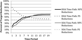
Distribution of Reductions by Pollution Source
Figures 4 and 5 show how much of the overall reduction in load comes from PS and NPS emissions for the 20-period SC and WC models, respectively, in the case of a constant load limit and no adjustment cost. Figures 6 and 7 show the same information for the 40-period SC and WC models, respectively. In both cases, the SOA allocates 40 percent of the reduction to PS emissions and 60 percent to NPS emissions in the steady state. Though the practices consistent with this allocation are implemented at the beginning of the implementation phase, the distribution is not realized until the steady state is achieved. Figures 4 through 7 reflect this; reduction of the NPS emissions increases gradually, reaching the steady-state level of 60 percent by the final period while reductions in PS emissions are constant at the steady-state SOA level. The DOA relies heavily on reductions from the PS in the early periods, when only a small portion of the NPS loads are present due to lags, and gradually shifts to reductions in the NPS over time.
Distribution of Nonpoint-source and Point-source Reductions: T = 20, No Adjustment Cost, Strong Correlation
Distribution of Nonpoint-source and Point-source Reductions: T = 20, No Adjustment Costs, Weak Correlation

Distribution of Nonpoint-source and Point-source Reductions: T = 40, No Adjustment Costs, Strong Correlation

Distribution of Nonpoint-source and Point-source Reductions: T = 40, No Adjustment Costs, Weak Correlation

The steady-state reductions in NPS and PS emissions under the DOA are similar to the reductions under the SOA but rely somewhat more on the PS in the SC model: 44 percent in the 20-period model and 48 percent in the 40-period model versus 40 percent under the SOA. The WC steady-state SOA reduction percentages are identical to those of the SC model, though NPS reductions increase in a more linear fashion in the WC model than in the SC model. When the correlation between the lags and delivery factors is weak, the DOA relies more heavily on reductions from the PS, with steady state reductions of 48 percent in the 20-period model and 54 percent in the 40-period model. This greater reliance on the PS even in the steady state is the result of differences in the optimality conditions for the allocations, which require that the marginal abatement cost for delivered pollution is greater for lagged NPS emissions than for the unlagged PS emissions.
Consistent with our discussion of the effects of correlation between lags and delivery factors on costs, the PS/NPS split tilts more toward NPS when the correlation is strong. WC effectively reduces the load reduction available from high-delivery-ratio bins in early periods compared to SC. In the SC model, the NPS reduction increases relatively rapidly in earlier periods and more slowly later; in the WC model, the percent reduction is essentially linear over time. The NPS reductions in the final period are always greater under SC than under WC because of the uneven distribution of short lag lengths to bins that have a high delivery factor in the SC model and the even distribution of lag lengths in the WC model.
Time Paths of Undiscounted Marginal Abatement Costs
The time paths of undiscounted marginal abatement costs are presented in Table 5 and selected results are illustrated in Figures 8 and 9 in the case of no adjustment cost. The marginal abatement costs under the SOA are constant for all periods at $5.45 per pound in both the 20-period and the 40-period model. Under the DOA, the marginal abatement costs start at $15.04 (20-period) and $16.33 (40-period) per pound in the SC model and $16.66 (20-period) and $17.23 (40-period) per pound in WC model. They decline over time to steady-state values of $6.16 (20-period) and $6.97 (40-period) per pound in the SC model and $6.96 (20-period) and $8.41 (40-period) per pound in the WC model.
Marginal Costs for Undiscounted Nitrogen: T = 20, No Adjustment Costs

Marginal Costs for Undiscounted Nitrogen: T = 40, No Adjustment Costs

Undiscounted Nitrogen Marginal Costs

The larger initial marginal abatement costs in the DOA reflect the limited capacity of NPSs to provide reductions in the delivered load. Consequently, the PS must make larger, more expensive reductions. Over time, greater reductions can come from NPSs, allowing the PS to increase its emissions and reduce costs. The undiscounted marginal abatement costs are lower in the SC model than in the WC model in every period and decrease more rapidly in the SC model in initial periods, again because of the implications of concentrating shorter lag lengths in bins that have high delivery factors.
Phosphorus Results
As noted earlier, we limit our discussion of the results for phosphorus emissions; the full results are available from the authors upon request. Because of the relatively long lags associated with phosphorus loads (see Table 1), we did not estimate 20-period models. As with nitrogen emissions, the cost of the implementation phase is significantly higher under the DOA with no adjustment cost than under the SOA for both strong (about 56 percent) and weak (about 63 percent) correlation. In the first period, both allocations attain approximately 74 percent of the required reduction regardless of correlation, which is significantly greater than the 55 percent attained in the nitrogen models. After period 19, the SC and WC models for phosphorus achieve 91 percent and 87 percent of the environmental target, respectively, compared to 91 percent and 76 percent, respectively, for nitrogen.
We also again find significant cost savings associated with the SOA for phosphorus. The DOA is 56 percent more expensive under SC and 63 percent more expensive under WC with a constant load limit and no adjustment cost, and the gap between the SC and WC models in the SOA's achievement is smaller for phosphorus. These results indicate that the interaction between lag length and the delivery factor is less significant for phosphorus.
Summary and Conclusions
This research is motivated by a need to understand the implications of lags in agricultural pollution for the efficiency and design of water-quality markets. Of particular interest is whether a simple market design under the assumption of contemporaneous substitution (i.e., no lags) can produce results that are reasonably comparable to those of more-complex and more-expensive dynamic designs that facilitate trading across time and space to address lags.
We first present conceptual models of efficient pollution-control allocations with and without lags to develop the key concepts and an analytical framework for the study and static and dynamic simulation models to compute static and dynamic optimal allocations of abatement effort to reduce nitrogen pollution in Chesapeake Bay. Given uncertainty associated with the durations of the lags and their spatial distributions, we use scenarios involving variations in the longest lag length in the model and spatial correlation between lag length and pollution-delivery coefficients.
We find that the length and spatial structure of the lags can have significant impacts on the cost of controlling pollution and the distribution of abatement efforts between PS and NPS emitters over time. These factors interact so the implications depend on the specific relationships.
Simple static rules that ignore lags in the delivery of pollution in a watershed allocate reductions in pollution to sources based on each source's marginal abatement cost without regard to the timing of the reductions and treat implementation of BMPs as if they are fully effective in the period in which they are implemented. For a target of a 24.5 percent reduction in the amount of pollution delivered to Chesapeake Bay, an SOA allocates approximately 60 percent of the reduction effort to NPSs and 40 percent to the PS, and those allocations are realized only after pollutants from sources that have the longest lags have already been delivered. Prior to that time, the actual emissions will exceed the load limit.
Dynamic allocation rules take lags in the distribution of pollution across sources and time into account. Thus, DOAs equalize the discounted marginal costs of reductions in the pollution delivered to the bay by accounting for the timing of those deliveries. Our simulations show that dynamic allocations rely more heavily on reductions by the PS to fully achieve the pollution target in initial years but gradually substitute lower-cost NPS reductions for the PS reductions over time until a steady-state allocation is achieved. The steady-state NPS and PS reductions approximate the reductions achieved by the SOA to varying degrees with somewhat greater reliance on abatement by the PS related to differences in the DOA and SOA optimality rules. The simulations demonstrate that the initial and steady-state allocations of abatement requirements depend on the length of the lags, correlation between the lag lengths and delivery factors, and the type of pollutant (reflecting differences in marginal abatement costs). They also depend on the discount rate, but we limited our analysis to the OMB rate of 7 percent.
Importantly, the SOA rules result in a significant cost saving relative to the DOA rules in all of the models, indicating that simpler static market designs are economically advantageous. Their downside is a delay in achieving the water-quality goals. However, we find that the SOA rules can obtain the targeted reductions in pollution reasonably quickly in our Chesapeake Bay application. In all scenarios we considered, the SOA achieved about 55 percent of the load reduction target for nitrogen pollution at the beginning of the implementation phase. When correlation between lag length and delivery speed is strong, the SOA achieves about 90 percent of the required reduction by period 9 in the 20-period model and period 19 in the 40-period model. When that correlation is weak, the SOA achieves about 75 percent of required nitrogen reductions by those periods. Thus, if the ultimate goal is to achieve a healthy level of water quality in Chesapeake Bay over the long term, the simple SOA is economically compelling compared to the more complex DOA. Of course, this assumes that all of the factors that affect pollution in the Chesapeake Bay watershed (such as land-use distributions and populations) remain constant over time.
The SOA is a simple design in that it economizes on information that would be required by the DOA. For example, calculation of the SOA does not depend on the spatial correlation between the lag lengths and the pollution-delivery coefficients, information that either is not available or is costly to obtain. The DOA cannot be calculated without that information. Because of the lack of such information for the Chesapeake Bay watershed, we took a scenario approach (modeling weak and strong correlation). The DOA could have been calculated using an estimate of correlation, but if the estimate was inaccurate, the result would not have the theoretical property we desired—it would not minimize the societal cost subject to meeting the load-limit constraint in each period.
It is important to note that the evolution of the SOA load path is not inconsistent with implementation of the Chesapeake Bay TMDL. Unlike the phased implementation of BMPs under the TMDL, the SOA requires immediate implementation of the control practices needed to achieve the targeted reduction in the pollution load in the steady state. The delays in reducing pollution are the result of the lags, not of implementation.
In summary, the results of this study suggest that the traditional emphasis on PSs for initial reductions in nutrient pollution is consistent with a dynamically efficient allocation. The results also suggest that the presence of lags in delivery of pollutants would lead to a relatively greater allocation to PSs over NPSs in the long run in dynamically efficient allocations compared to static efficient allocations. Finally, we find that static efficient allocations save money and can perform reasonably well environmentally, suggesting that simpler market designs that do not explicitly account for lags can be appropriate for water-quality trading.
This work contributes to a better understanding of the implications of lags in the delivery of agricultural pollution for efforts to cost-effectively reach target reductions in pollution and improve water quality. Future research can consider a comprehensive analysis of economically optimal paths that address the various dynamics that influence the cost of damage from pollution, such as lags in ecosystem responses to reduced pollution, the persistence of pollutants, and positive feedback from phosphorous concentrations.


 Open access