

Introduction
Supraglacial lakes (SGLs), which form from the pooling of runoff in topographic depressions, are an annual feature on the Greenland ice sheet (GrIS) during the melt season. SGLs locally decrease the surface albedo with respect to the neighbouring bare ice area, accelerating melting as a result (Reference Greuell, Reijmer and OerlemansGreuell and others, 2002). In recent years, SGLs have been the subject of both observational (e.g. Reference McMillan, Nienow, Shepherd, Benham and SoleMcMillan and others, 2007; Reference DasDas and others, 2008; Reference Selmes, Murray and JamesSelmes and others, 2011; Reference DoyleDoyle and others, 2013) and modelling studies (e.g. Reference Lüthje, Pedersen, Reeh and GreuellLüthje and others, 2006; Reference Banwell, Arnold, Willis, Tedesco and AhlstrømBanwell and others, 2012; Reference Leeson, Shepherd, Palmer, Sundal and FettweisLeeson and others, 2012) due to their ability to impact ice-sheet dynamics. SGLs drain rapidly through hydrofracture (Reference Van der VeenVan der Veen, 2007; Reference Krawczynski, Behn, Das and JoughinKrawczynski and others, 2009), and the timing of peak lake drainage has been linked to the timing of seasonal speed-up of the ice sheet (Reference Shepherd, Hubbard, Nienow, McMillan and JoughinShepherd and others, 2009; Reference Bartholomew, Nienow, Mair, Hubbard, King and SoleBartholomew and others, 2010). However, it is uncertain whether an increase in either the number of, or volume of water from, draining SGLs will result in a net acceleration of the ice sheet (Reference SchoofSchoof, 2010; Reference Sundal, Shepherd, Nienow, Hanna, Palmer and HuybrechtsSundal and others, 2011). SGLs continue to be studied due to their role in the supraglacial hydrological network. In particular, the location of SGLs is of interest due to their potential to enable surface-to-bed connections, where conduits such as moulins and crevasses are rare, for example at high elevations (Reference BartholomewBartholomew and others, 2011; Reference Howat, De la Peña, Van Angelen, Lenaerts and Van den BroekeHowat and others, 2012). Additionally, knowledge of SGL volume is desirable to constrain the amount of water available for hydrofracture and subsequent rapid delivery to the base of the ice sheet (Reference Leeson, Shepherd, Palmer, Sundal and FettweisLeeson and others, 2012).
Traditionally, observations of lake behaviour are made in situ or are obtained remotely using satellite instruments such as the Advanced Spaceborne Thermal Emission and Reflection Radiometer (ASTER), the Moderate Resolution Imaging Spectroradiometer (MODIS) and the Landsat-7 Enhanced Thematic Mapper Plus (ETM+) (e.g. Reference Box and SkiBox and Ski, 2007; Reference Sneed and HamiltonSneed and Hamilton, 2007; Reference Georgiou, Shepherd, McMillan and NienowGeorgiou and others, 2009; Reference Sundal, Shepherd, Nienow, Hanna, Palmer and HuybrechtsSundal and others, 2009; Reference Tedesco and SteinerTedesco and Steiner, 2011). SGLs are identified in satellite images obtained using these optical remote-sensing instruments by manual interpretation, where each lake is digitized by hand (e.g. Reference McMillan, Nienow, Shepherd, Benham and SoleMcMillan and others, 2007; Reference Georgiou, Shepherd, McMillan and NienowGeorgiou and others, 2009), and by semi- or fully automated methods (e.g. Reference Sundal, Shepherd, Nienow, Hanna, Palmer and HuybrechtsSundal and others, 2009; Reference LiangLiang and others, 2012). ASTER and ETM+ images have a high spatial resolution (of the order ∼10 m), conducive to accurate lake area delineation, but MODIS imagery is much coarser (250 m). However, the MODIS image record has a far higher temporal sampling (at least once a day rather than biweekly) and is better able to resolve the evolution of lakes, i.e. the initiation, growth, shrinkage and disappearance of lakes as the melt season progresses. Typically, studies of SGL evolution at both annual and interannual timescales are investigated using MODIS (e.g. Reference Selmes, Murray and JamesSelmes and others, 2011; Reference Johansson, Jansson and BrownJohansson and others, 2013) because of its relatively dense temporal sampling. However, in years of abundant cloud cover, the record may contain as few as 12 completely cloud-free images during a single melt season (Reference Sundal, Shepherd, Nienow, Hanna, Palmer and HuybrechtsSundal and others, 2009).
SGLs are found predominantly in the ablation zone of the GrIS and are particularly abundant in the southwest (Reference Selmes, Murray and JamesSelmes and others, 2011). The impact of rapid lake drainage on seasonal and shorter-term ice-sheet dynamics in this region, particularly in the Russell Glacier catchment, is well documented (Reference Shepherd, Hubbard, Nienow, McMillan and JoughinShepherd and others, 2009; Reference Palmer, Shepherd, Nienow and JoughinPalmer and others, 2011). Three independent observational studies of SGL evolution in the Russell Glacier region have been performed (Reference Sundal, Shepherd, Nienow, Hanna, Palmer and HuybrechtsSundal and others, 2009; Reference Selmes, Murray and JamesSelmes and others, 2011; Reference Johansson and BrownJohansson and Brown, 2013) using three different automated lake classification systems to report the location and size of lakes in MODIS imagery. In these studies, the performance of these automated classification algorithms was evaluated by comparing a sample of automatically delineated lakes from a MODIS image against a sample of lakes delineated manually from contemporaneous, or nearly contemporaneous, high-resolution ASTER or ETM+ imagery. For example, Reference Sundal, Shepherd, Nienow, Hanna, Palmer and HuybrechtsSundal and others (2009) used 53 lakes featured in a single ASTER image taken on 1 August 2001, Reference Selmes, Murray and JamesSelmes and others (2011) used 100 lakes identified in multiple ASTER scenes over a 3 year period across two regions of the ice sheet, and Reference Johansson and BrownJohansson and Brown (2013) used all lakes in seven Landsat-7 (ETM+) images acquired 1–6 days prior to/ after the acquisition of four MODIS images over 2 years (276 lakes in total). The relative scarcity of cloud-free MODIS and ASTER or ETM+ images means that few days exist where an in-depth evaluation may be made using data acquired on exactly the same day.
In this paper, we perform an extensive intercomparison of automatically derived SGLs using the datasets of Reference Sundal, Shepherd, Nienow, Hanna, Palmer and HuybrechtsSundal and others (2009; hereafter Sundal09), Reference Selmes, Murray and JamesSelmes and others (2011; hereafter Selmes11) and Reference Johansson and BrownJohansson and Brown (2013; hereafter Johansson13). First, we investigate the effect of temporal sampling on quantitative estimates of (1) the date of first appearance of any lake (onset day); (2) the maximum area covered by all lakes observed (maximum lake area); (3) the elevation of the highest lake on the ice sheet (maximum elevation); and (4) the total number of times any lake is observed (number of lake appearances). Second, we evaluate the performance of the three automatically derived datasets in terms of reporting (1) the number of lakes on any given day (daily number of lakes), and (2) individual lake area (lake area) compared with a dataset of lakes derived by manual classification of the same MODIS images. Third, we evaluate the performance of Sundal09 and Johansson13 in terms of calculating lake area compared with manual classification of corresponding ASTER imagery. Finally, we combine Sundal09, Selmes11 and Johansson13 into a single optimized dataset. This new dataset includes more days of data that are completely cloud-free, and/or more lakes on each of these days, than Sundal09, Selmes11 and Johansson13 individually. This dataset is ultimately used to investigate the interannual variability in SGL evolution during the period 2005–07. This period can be considered climatically representative since it encompasses one high (2007), one low (2005) and one moderate (2006) runoff year according to simulations performed using the Modèle Atmosphérique Régional (MAR) regional climate model (Reference FettweisFettweis, 2007) forced by the European Centre for Medium-Range Weather Forecasts (ECMWF) Interim Re-analysis (ERA-Interim).
Data and Methods
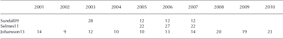
This study focuses on a 16 000 km2 area of the west GrIS, ranging from the margin to ∼1750 m a.s.l., in the region of Russell Glacier. Sundal09 and Johannson13 focused on this region only and restricted their records to data derived from MODIS images that had been identified manually as completely cloud-free. For each day on which a cloud-free image was identified, each dataset includes a map of SGLs that had been delineated automatically from a single image (a daily SGL distribution). Selmes11 consists of individual lake images documenting the evolution of 2600 individual lakes over 3 years from all regions of the GrIS, of which ∼231 are in our study region. These data include partially cloudy as well as cloud-free days. In this study, on days that we identify manually as cloud-free, we mosaic together daily SGL distributions from these individual lake images. Table 1 indicates the number of daily SGL distributions in each dataset for each year where observations are available. We next provide a brief description of each method; the reader is referred to the appropriate publication for additional details.
Number of days used to compile automatic datasets of supraglacial lake evolution. Where a number is absent, no observations are available in that dataset in that year. The abbreviations refer to observations derived using the methods of Reference Sundal, Shepherd, Nienow, Hanna, Palmer and HuybrechtsSundal and others (2009), Reference Selmes, Murray and JamesSelmes and others (2011) and Reference Johansson and BrownJohansson and Brown (2013)
Sundal09 and Johansson13 delineated lakes automatically using object-oriented segmentation and classification methods. Sundal09 assigned objects a ‘lake’ or ‘non-lake’ status based on the degree to which they belong to the lake or non-lake class, in terms of reflectance. Johansson13 extended this method of classification to include size, shape and brightness, in addition to reflectance. They also allowed the threshold values of each parameter to evolve with season. Selmes11 operated from an a priori assumed lake distribution, considering each known lake location in turn. At each location, pixels were assigned lake or non-lake status based on whether their reflectance exceeded 65% of the mean value in a standard reference window. The methods each used the same MODIS images in their classification of lakes; Sundal09 used bands 1 and 3 of these images, Selmes11 used band 1 only and Johansson13 used bands 2 and 4. Each method was found to exhibit sources of uncertainty. For example, Sundal09 had difficulty resolving ice-covered lakes and may accordingly underestimate total lake-covered area by as much as 21.1% (Sundal, unpublished information). In Selmes11, any lake either not included in the a priori distribution or <0.125 km2 does not feature in the dataset. Finally, Johansson13 reported that as many as 18% of reported SGLs are likely to be false positives (objects categorized initially as lakes, but which may be reassigned to the non-lake category upon further inspection (e.g. after reference to an image with higher spatial resolution)). An example of lake delineation by each method is given in Figure 1.
Comparison of manually and automatically derived lake distributions on 14 June 2005 (day 165) in a small subsection of the study region. Background is the original MODIS image. In (a) circles surround SGLs identified manually. Squares in (b) and (d) illustrate lakes reported in a single dataset. In (c) the triangle indicates an ice-covered lake and the semicircle indicates an ice-free lake, neither of which is identified by any of the three automatic lake detection algorithms. The diamond in (d) indicates a reported lake that has been identified as a false positive.

SGLs have been observed to disappear by draining rapidly in just a few hours (Reference DasDas and others, 2008; Reference DoyleDoyle and others, 2013). However, the temporal sampling of satellite datasets is typically sparse by comparison (Table 1). To investigate the impact that temporal sampling has on assessments of SGL evolution, we systematically subsample daily SGL distributions from the most populous lake dataset and compute key metrics from successively smaller samples. For this exercise, we use the Sundal09 dataset acquired in 2003, as this is the most densely sampled, with 28 separate daily SGL distributions. For each subsample size (5–27), we randomly select 1000 subsamples of this size, from the 28 day record. For example, considering a sample size of 5, 1000 separate sets of 5 different daily distributions, randomly chosen from all available (28) daily distributions, are selected. The mean, standard deviation and range of values of four key SGL characteristics among each set of 1000 subsamples are then calculated and compared. The SGL characteristics selected for this analysis are the maximum lake area (km2), the onset day, the maximum elevation (m a.s.l.) and the number of lake appearances.
Supraglacial lake identification algorithms exhibit differences in performance. To assess this difference, we compare the size and daily number of SGLs reported in each automatically derived dataset with estimates derived from manual classifications. The manual classifications are developed from MODIS data acquired in each year of overlap between the three automatically derived datasets (2005, 2006 and 2007). First, the areas of ten lakes, exhibiting a range of size and shape, are delineated by three different people using satellite images acquired on two different days, in each year. These particular lakes were chosen as they were the only lakes reported in two or more daily distributions, in all three years, by all three datasets. Pixels reported to be lakes in two or more of the manual delineations, for any given day, are identified as SGLs. Next, maps of SGL distribution are created by three people, each on the same nine separate days corresponding to early, mid-and late melt season in each of the three years. Features reported as lakes in two or more of these manual distributions are identified as SGLs (78% of all features identified). Finally, we quantify the performance of each automatically derived dataset in reporting SGLs as a linear sum of their skill in reporting lake area and daily number of lakes as compared with the manual datasets. Skill is characterized by the relative performance, P, of each automatically derived dataset, j, calculated using the rootmean-squared deviation (RMSD) from the manually derived data and using

Because MODIS imagery has a coarse spatial resolution (250 m), we assess the relative performance of our method of manually classifying MODIS imagery, and the automated methods employed by Sundal09 and Johansson13, by comparison with ASTER data. In order to perform this analysis, a sample of 45 lakes is manually delineated, using the method described above, from ASTER imagery acquired on 1 August 2001. The same 45 lakes are also manually delineated from a contemporaneous MODIS image.1 August 2001 is the only day for which both MODIS and ASTER data were available, and which features in two or more of the automatically derived datasets; Selmes11 is not included in this analysis because this dataset does not include data for this day. No ASTER data are available for common days between all three datasets.
We combine results of the three automatically derived SGL datasets, using a hierarchical scheme based on their relative performance in reporting lake area and daily number of lakes, to form a single SGL index for the period 2005–07. In this hierarchical dataset, lakes are mapped on each date when two or more observations were available. Firstly, lakes from the dataset with the highest performance are incorporated. Next, all lakes from the dataset with the second highest performance, and which do not feature in the dataset with the highest performance, are included. Finally, lakes from the dataset with the lowest overall performance are similarly incorporated into the combined record. Because automatic methods of identifying SGLs in satellite imagery are known to produce false positives (Reference Johansson and BrownJohansson and Brown, 2013), we also estimate the frequency of false positives in each dataset by comparison with a sample of manually classified SGLs.
Results
Impact of temporal sampling on reported lake evolution
Subsampling of the satellite imagery shows that sparsely sampled datasets can fail to capture key aspects of SGL evolution (Fig. 2). If the sample size is limited to 10 days (the smallest sample size featured in the automatically derived datasets), the estimated onset date can be delayed by up to 41 days, the estimated maximum area can be underestimated by up to 287%, the maximum elevation can be underestimated by as much as 180 m a.s.l. and the total number of lake appearances can be underestimated by as much as 60% (Fig. 3). These extreme deviations from ‘true’ values arise as a result of clustering around a few dates within a sample. On average, a sample size of 10 days underestimates the maximum lake area, onset date, maximum elevation and the number of lake appearances by 16%, 4 days, 3 m a.s.l. and 23%, respectively (Table 2).
Mean and standard deviation, associated with sample size, of reported maximum lake area, onset day, maximum elevation and number of lake appearances in 2003. Sample size refers to the number of daily SGL distributions in that sample

Impact of temporal sampling on reported SGL evolution in 2003. Seasonal variability in lake-covered area is reported using sample sizes of 5, 10, 15, 20 and 25 daily lake distributions and the full data record of 28 days. Shaded regions indicate the spread of values associated with each sample size as achieved using 1000 random samples. Shaded squares indicate the latest possible onset day using that sample. Point data are connected by linear interpolation.

Detailed impact of temporal sampling on reported SGL evolution in 2003. (a) Range of maximum lake area reported by taking 1000 samples each of sizes 5–27 daily SGL distributions, with respect to that reported using a sample of 28 days. Mean value is indicated using ‘x’; error bars on this value refer to one standard deviation (1SD) on reported values and are truncated by the value calculated using the full 28 day sample (dotted horizontal line). The minimum value reported using a given sample size is marked with ‘+’. (b) Same as (a) but for onset day; this value is overestimated when calculated using a smaller sample, with reference to a 28 day record. (c) Same as (a) but for maximum elevation. (d) Same as (a) but for number of lake appearances reported.

Lake area derived from MODIS vs lake area derived from ASTER
The area of lakes manually delineated from MODIS images are found to have an RMSD of 0.24 km2 from lake area manually delineated from contemporaneous ASTER data. By comparison, the RMSD between lake area reported by Sundal09 and Johansson13 and lake area manually delineated from ASTER data is found to be 0.39 and 1.47 km2. No observations of SGLs contemporaneous with the ASTER data are available using the Selmes11 method and so an assessment of this algorithm’s performance against ASTER is not possible.
Intercomparison of supraglacial lake evolution as reported in three datasets based on MODIS imagery
Each of the three automatic classification methods leads to slightly different SGL distributions (e.g. Fig. 1). For example, no single method reports all the lakes identified manually; tracking ice-covered lakes is a problem for all three methods, and each dataset includes false positives. We calculate the total number of lakes reported in each year using combinations of the individual datasets (Fig. 4). Combining datasets leads to an increase in the number of lakes reported: for example, when combined, Johansson13 and Selmes11 include up to 70% more lakes than Selmes11 (the dataset reporting the least number of lakes) alone.
Number of lakes reported in each year using combinations of datasets.

Sundal09, Selmes11 and Johansson13 report 796, 566 and 934 lake appearances in nine separate MODIS images across the 3 year period. However, compared with SGL distributions derived manually from the same data, each dataset is found to feature false positives: 61 (9%), 27 (5%) and 322 (33%), respectively. When false positives are excluded, the Sundal09, Selmes11 and Johansson13 data-sets report 71%, 52% and 59% of the manually identified lakes. The RMSD between the daily number of positively identified lakes in the datasets derived automatically and manually are found to be 40, 64 and 61 lakes, respectively.
We compare lake area, as reported by Sundal09, Selmes11 and Johansson13, with a sample of 60 individual lake images delineated manually from original MODIS data, and find mean biases of −27%, −4% and +55%. However, the variability in all cases is high and neither Sundal09 nor Selmes11 consistently reports lake area one standard deviation (1SD) away from values reported in the sample delineated manually (Fig. 5). The RMSD between the area of lakes delineated automatically and manually is found to be 0.78, 0.48 and 0.95 km2 for Sundal09, Selmes11 and Johansson13. The relative performance of the Sundal09, Selmes11 and Johansson13 datasets overall is found to be 0.72, 0.75 and 0.53, respectively, where a higher score indicates a better performance (Table 3).
Comparison between automatically derived area and manually delineated area of 60 separate lake images acquired during 2005–07. Shaded regions relate to a linear fit ±1SD. Hatched region indicates a one-to-one fit ±1SD uncertainty in the manually delineated sample.

Intercomparison of automatically delineated SGLs with manually delineated SGLs, both from MODIS data acquired in 2005–07. RMSD values are transformed into a relative performance score for each dataset, with respect to each parameter. An overall performance score is calculated for each dataset as the linear sum of these scores

A combined dataset of supraglacial lake evolution
When the three automatically derived SGL datasets are combined, on average 67% more lakes are reported on each day than are reported by the dataset that contains the lowest number of lakes (Selmes11) (Fig. 6). The combined dataset also includes more daily SGL distributions than the dataset that features the lowest number of days overall (Sundal09). For example, in 2005, 2006 and 2007, the combined dataset includes 15, 19 and 17 days compared with 12, 12 and 12 days in Sundal09. Onset day is delayed, on average, by 4 days using a sample size of 12 (Fig. 3). For a sample size of 19, this delay is reduced by half to 2 days. The mean underestimate of maximum elevation is reduced from 3 m a.s.l. (which, on average, encompasses an area of 30.42 km2 in this study region) when a sample size of 12 is used to 0.5 m a.s.l. (4.95 km2) with a sample size of 19. Maximum lake area is underestimated by 16% and 5% on average, and the number of lake appearances is underestimated by 23% and 15% on average, when sample sizes of 12 and 19 are used, respectively.
Interannual variability of SGL evolution using a new SGL index for 2005–07. Rows are time series of (a) mean lake area, (b) total lake-covered area and (c) daily number of lakes, for 2005, 2006 and 2007. Sundal09 is indicated by diamonds, Selmes11 by squares, Johansson13 by triangles and the combined dataset by filled circles. The shaded region delineates a linear (mean area) or Gaussian (total area and daily number of lakes) fit to the combined dataset, including the 1SD uncertainty on this fit. Also shown (black curve) is the total daily runoff (km3 d−1) integrated over the study region, as simulated by the MAR model (Reference FettweisFettweis, 2007).

There is considerable interannual variability in spatially integrated SGL characteristics in the combined (optimized) SGL dataset during the three years under consideration (Fig. 6). For example, maximum lake area is found to be 166, 214 and 132 km2 in 2005, 2006 and 2007. The rate of lake area growth in all three years (6, 5 and 10 km2 d−1) approximately follows the rate of change of runoff production. For example, at the beginning of the melt season in 2007, runoff production accelerates quickly and we see a corresponding rapid growth in total lake area. In 2007, the widespread disappearance of lakes occurs sooner than in 2005 and 2006 (day 181, day 189 and day 170 for 2005, 2006 and 2007, respectively). Lake-covered area remains small in 2007 following this widespread drainage, despite continued runoff production. In addition, lake onset and progression inland/up the ice sheet occurs earlier in 2007 than in either 2005 or 2006 (Fig. 7).
Variation of onset day with distance from margin in (a) 2005, (b) 2006 and (c) 2007. Symbols indicate dataset: Sundal09 is indicated by diamonds, Selmes 11 by squares and Johansson13 by triangles. The combined dataset is given by a solid line. Here error bars indicate uncertainty due to temporal sampling.

Discussion
Impact of temporal sampling on reported lake evolution
Satellite imagery allows large areas of the ice sheet to be studied simultaneously, which enables insight into regional patterns of SGL evolution (e.g. Reference Sundal, Shepherd, Nienow, Hanna, Palmer and HuybrechtsSundal and others, 2009). However, we find that in a dataset derived solely from MODIS data, uncertainty due to temporal sampling of the satellite imagery is inversely proportional to the number of images used to compile an annual record of SGL evolution. This is not surprising, because rapid lake drainage can occur over timescales of the order of hours (e.g. Reference Selmes, Murray and JamesSelmes and others, 2013) and in this region of the GrIS approximately half of all lakes have a lifespan of <10 days (Reference Johansson, Jansson and BrownJohansson and others, 2013). We also find that uncertainty increases dramatically when there is clustering within a sample, presumably because lakes that are likely to have grown and drained on days outside the cluster are not included in the record.
Entirely cloud-free MODIS images can be scarce, particularly prior to 2008 (Table 1), and tend to be clustered. However, lakes can also be observed using synthetic aperture radar (SAR), which can penetrate cloud (Reference Johansson, Brown, Jansson and Lacoste-FrancisJohansson and others, 2011). Although the temporal resolution of the SAR image record can be coarse relative to MODIS (e.g. TerraSAR-X has a repeat time of 11 days), these data could be used to supplement the optical record during periods of persistent cloud cover. In order to reduce the mean under-/ overestimate of all four lake characteristics considered to within 5% of the value calculated using a 28 day record, at least 20 images in total are required (Fig. 3). These images ought to be distributed uniformly throughout the year to minimize the risk of increased uncertainty due to clustering. For a melt season of 130 days in duration, this enables the date of initiation and demise of individual lakes to be reported to within 6.5 days of the true value.
Selmes11 and Reference LiangLiang and others (2012), track individual lakes rather than large areas, allowing partially cloudy images to be exploited and generally more lake initiation/ drainage events to be captured at a temporal resolution that is finer than available using entirely cloud-free images. Even so, because of the possibility of cloud cover, the evolution of specific lakes cannot always be captured at a useful resolution using this method. Field-based monitoring allows sufficiently dense temporal sampling of lake evolution to report the beginning of rapid drainage to within a few seconds (e.g. Reference DasDas and others, 2008; Reference DoyleDoyle and others, 2013). As a result, where particular lakes are of interest (e.g. example because of the risk of downstream effects of rapid drainage), remote-sensing data can be considered complementary to field-based monitoring rather than as a replacement for in situ measurements.
Manual delineation of lake area vs automated delineation of lake area
When compared with lakes delineated manually from ASTER imagery, manual delineation of MODIS imagery is found to report lake area more accurately than the automated methods of Sundal09 and Johansson13. However, on average, lake area delineated manually from MODIS imagery can deviate by as much as 0.24 km2 from values calculated using ASTER. This can be attributed to the difference in spatial resolution between the MODIS and ASTER instruments (250 and 15 m, respectively) and suggests that ASTER imagery ought to be used preferentially when compiling a multi-source record of SGL evolution.
Although manual delineation of lake area is more accurate, automated classification is significantly less time-consuming. Using the method described here, it takes ∼4 man-hours to manually delineate all lakes in a single MODIS image. In contrast, the Selmes11 method is able to automatically delineate all the SGLs in a single MODIS image on a timescale of the order of minutes. As a result, manual delineation is most useful for evaluating automated methods and for augmenting field observations, which typically consider small numbers of lakes on short timescales.
Intercomparison of supraglacial lake evolution as reported in three datasets based on MODIS imagery
The performance of three independent SGL datasets derived from MODIS imagery is assessed by comparison with data delineated manually. Of the three datasets, Selmes11 is found to report lake area most accurately, with respect to manually derived lake area. This suggests that the Selmes11 method of lake delineation, i.e. considering each pixel in turn at a known lake location and assigning it lake/non-lake status based on a threshold reflectance value, is best able, of the three techniques, to report lake area. That said, the Selmes11 method was also found to report the smallest number of lakes identified manually (52%). A possible explanation for this under-reporting is the fact that the Selmes11 procedure excludes lakes that are small and that do not feature in a predefined target distribution. The Sundal09 dataset is found to report the highest number of lakes identified manually on each day, which suggests that the Sundal09 approach to identifying lake locations, i.e. by object-oriented segmentation and classification, is best able to map the distribution of lakes in each MODIS image.
Each of the three automatically derived datasets is also shown to include false positives, ranging from 5% to 33% for Selmes11 and Johansson13, respectively. For comparison, Johansson13 estimate that their dataset contains up to 18% false positives. Possible explanations for the approximately twofold increased rate of false positives reported here include the relatively coarse temporal separation of the evaluation data used by Johansson13, and the relatively coarse spatial resolution of the evaluation data used here. Johansson13 is found to perform least well in terms of reporting lake area, overestimating by 55% on average. A possible explanation for this overestimate is the fact that their procedure employs optical data acquired in the wavelength range 545–565 nm (MODIS band 4), which is known to be overly sensitive to shallow water (Reference Sneed and HamiltonSneed and Hamilton, 2007).
Based on these findings, we recommend that future studies utilizing automated classification of SGLs adopt the Sundal09 approach to identifying lakes in MODIS imagery of bands 1 and 3, prior to delineating lake area using the Selmes11 method. By doing this, future studies can expect to report the size of 71% of lakes that can be identified manually to within 0.48 km2 of manually delineated lake area.
A combined dataset of supraglacial lake evolution
By combining the three datasets of Sundal09, Selmes11 and Johansson13, we achieve an increase in sampling of up to 58% more days in each year and up to 67% more lakes on each day. As a consequence of including more lakes, estimates of spatially integrated SGL characteristics (e.g. daily lake-covered area) using the combined (optimized) dataset may be considered more robust than those made using a single dataset. In addition, including more days of data offers a reduction in uncertainty due to sample size in terms of onset day, maximum elevation, maximum lake area and number of lake appearances (Table 2).
Using the combined (optimized) dataset, we find that in 2007, a particularly high runoff year, lake onset begins sooner, lake filling rate is more rapid and progression up the ice sheet/inland occurs earlier in the year than in the low and moderate runoff years of 2005 and 2006. Reference Johansson, Jansson and BrownJohansson and others (2013) calculated that a threshold value of melting has to be exceeded for lakes to form; these data suggest that this threshold was exceeded sooner in 2007 than in 2005 and 2006. Here there is no apparent correlation between annual runoff amount and observed maximum lake area, despite the suggestion by Reference Sundal, Shepherd, Nienow, Hanna, Palmer and HuybrechtsSundal and others (2009) that in a higher runoff year one might expect to observe a greater maximum lake area. Our findings support those of Reference LiangLiang and others (2012) who found no statistically significant correlation between melt intensity and maximum lake area in 10 years of data, including the period 2005–07.
It is likely that the high volume of runoff produced early in the melt season (Fig. 6) triggered the onset of widespread rapid drainage earlier in 2007 than in 2005 and 2006 (Reference LiangLiang and others, 2012). In 2007, following the onset of widespread drainage, lake-covered area remains small despite continued runoff production. This suggests that conduits linking the ice-sheet surface and base were established by hydrofracture during this time and then remained open for the remainder of the melt season, inhibiting further lake formation and growth. This phenomenon has been observed previously in field studies of individual lakes (e.g. Reference DasDas and others, 2008; Reference DoyleDoyle and others, 2013), and the data presented here imply that it also has an impact on lake-covered area at the regional scale. This behaviour is less apparent in 2005 and 2006, which may be attributed to the smaller proportion of lakes that disappeared through rapid drainage in these years compared with 2007 (Reference Selmes, Murray and JamesSelmes and others, 2013). It is also possible that in lower melt years insufficient meltwater is produced to keep surface–bed conduits open.
This study supports the findings of previous investigations (e.g. Reference LiangLiang and others, 2012; Reference Selmes, Murray and JamesSelmes and others, 2013) in that we observe interannual variability in SGL characteristics at the regional scale, particularly with respect to the impact of drainage processes. However, the findings discussed here are based on just 3 years of satellite data covering a relatively small region and would benefit from investigation using a more extensive record, both in space and time. Alternatively, it may be appropriate to use a model of SGL evolution (e.g. Reference Leeson, Shepherd, Palmer, Sundal and FettweisLeeson and others, 2012), in conjunction with spatially and temporally sparse observations, in order to investigate longer-term variability in SGL evolution, particularly in response to changes in climate.
Conclusions
We have investigated SGL evolution within three datasets, derived using automated classifications of satellite imagery, over a common 3 year period. Our results reveal a strong dependence of reported values of maximum lake area, onset date, maximum elevation and number of lake appearances on the number of satellite images used to compile an annual record of SGL evolution.
Manual delineation of lakes in MODIS imagery is found to be more accurate than automatic delineation when compared with contemporaneous ASTER imagery. Of the three datasets considered here, Selmesl 1 is found to report lake area most accurately (RMSD = 0.48 km2) and Sundal09 is found to report the number of lakes on each day most accurately (RMSD = 40 lakes), when compared with lakes delineated manually from MODIS imagery.
Based on our findings we recommend for future studies, firstly, that one image per 6.5 days is required in order to minimize uncertainties associated with poor temporal sampling. Secondly, we recommend that, where possible, records of SGL evolution are generated using ASTER or other imagery with similarly high spatial resolution (e.g. Landsat-7 ETM+), since these data offer a significant improvement in spatial resolution over MODIS (15 m compared with 250 m). Finally, we recommend that, where MODIS imagery is used, lakes should be automatically derived from band 1 or band 3 of these images using a combination of the methods of Sundal09 and Selmes11.
In the absence of a dataset that is densely sampled in time, we show that by combining all three datasets, more lakes that are identified manually are reported each day and uncertainty due to sample size is significantly reduced. In this combined (optimized) dataset, we note differences in spatially integrated SGL characteristics between years, such as the lake-covered area growth rate and the onset of drainage, which can be attributed to differences in runoff availability. However, this study considers only 3 years of data. More years of densely sampled observations or a long time series of SGL evolution simulated using a model will lead to improved confidence in this assessment.
Acknowledgements
This work was supported by a PhD studentship awarded to A.L. by the UK Natural Environment Research Council (NERC) National Centre for Earth Observation. A.L. thanks Lawrence Jackson for scientific discussion.


