


1. Introduction
The Great Depression was the most severe economic disruption in the history of the United States (US) and the downturn rippled through all aspects of society. While cross-sectional analyses suggest that fertility rates tend to be inversely related to income – such that poorer nations, or regions within them, generally exhibit higher fertility rates, ceteris paribus – fertility has been shown to be procyclical in more developed economies (Becker, Reference Becker and Roberts1960; Sobotka et al., Reference Sobotka, Skirbekk and Philipov2011). The Great Recession of 2008 had a particularly strong adverse (procyclical) impact on fertility rates worldwide (Goldstein et al., Reference Goldstein, Kreyenfeld, Jasilioniene and Örsal2013; Atysiak et al., 2021; Puig-Barrachina et al., Reference Puig-Barrachina, Rodríguez-Sanz, Domínguez-Berjón, Martín, Luque, Ruiz and Perez2020; Matysiak et al., Reference Matysiak, Sobotka and Vignoli2021). Coskun and Dalgic (Reference Coskun and Dalgic2024) argue that rising breadwinner status of women can explain both the emergence of procyclical fertility and the decline in fertility rate since the 1970s. Schaller et al. (Reference Schaller, Fishback and Marquardt2020) provide further historical evidence, finding that U.S. fertility has been procyclical since at least 1943. Is it possible that U.S. fertility was not procyclical during the 1930s?
In this paper, we examine the cyclical nature of fertility rates during the Great Depression in the United States using a fixed effects model that estimates the elasticity between state real personal income per capita and fertility rates during the interwar period. Our main results suggest that a one percent increase in state personal income per capita is associated with a 0.17 to 0.25 percent increase in fertility the next year. This result is robust to the inclusion of linear state time trends as well as time trends for a host of other demographic variables. We find that this estimated elasticity is also robust to the inclusion of state-level New Deal spending per capita as well as when estimating the dynamic effects of the percentage change in retail sales per capita between 1929 and 1933.
Interest in the demographic consequences of the Great Depression dates back to the event itself. Galbraith and Thomas (Reference Galbraith and Thomas1941) found a positive relationship between business cycles, measured using a national factory employment index, and births between 1919 and 1937 for five northeastern states. Kirk (Reference Kirk1960) shows that deviations in national fertility rates around a time trend are positively correlated with deviations in national industrial production around a time trend during the 1920s and 1930s. Still, Greenwood et al. (Reference Greenwood, Seshadri and Vandenbroucke2005) point out that there was no major structural break in national time series fertility associated with the Great Depression.Footnote 1 The birth rate in the United States had already been trending downward before the Great Depression occurred and that this downward trend ended around the time of the Great Depression. Still, Jones and Schoonbroodt (Reference Jones and Schoonbroodt2016) estimate a structural model using national data and find that the Great Depression led to a large baby bust during the 1930s. Insofar as state income per capita can measure the business cycle, this paper adds to this literature by directly examining the relationship between the business cycle and fertility with respect to the largest business cycle movement in United States history. What differentiates our paper from most of the literature is that we do not rely on national time-series data but instead use both state-level and county-level birth rates for all states and counties in the U.S.
Obviously, the literature on the pro-cyclical nature of fertility extends beyond the Great Depression. Puig-Barrachina et al. (Reference Puig-Barrachina, Rodríguez-Sanz, Domínguez-Berjón, Martín, Luque, Ruiz and Perez2020) shows that the Great Recession circa 2008 negatively impacted Spain’s fertility rate in the years immediately followed it. Goldstein et al. (Reference Goldstein, Kreyenfeld, Jasilioniene and Örsal2013) finds that across the whole of Europe, those countries that were hit hardest by the Great Recession saw the largest negative shocks to fertility, and these effects were strongest amongst younger cohorts. Matysiak et al. (Reference Matysiak, Sobotka and Vignoli2021) explores the relationship between fertility and economic conditions across 251 European regions in 28 European Union member states from 2002 to 2014 and finds that the periods of economic downturns – including the Great Recession – are associated with negative fertility dynamics. These findings are consistent with the well-established pre-Great Recession findings that fertility decisions are procyclical (Hondroyiannis, Reference Hondroyiannis2010; Orsal and Goldstein, Reference Orsal and Goldstein2010).
Our paper is most similar to Schaller et al. (Reference Schaller, Fishback and Marquardt2020), who also use county-level birth rates and per capita income to estimate the procyclical nature of fertility. We find that the relationship between state-level personal income per capita and fertility rates remains broadly stable across the pre- and post-World War II periods, though the dynamic responses are more muted in the earlier era. We further extend the analysis by examining how volatility in economic growth influences fertility behavior.
Fishback et al. (Reference Fishback, Haines and Kantor2007) examine how New Deal spending impacted fertility decisions in major US cities between 1929 and 1940. While the effect of the New Deal on fertility is not the primary focus of our paper, we show that the inclusion of controls for New Deal spending does not change any of our results.
Our paper is also situated within a broader literature focused on the how the Great Depression impacted various socioeconomic outcomes. Hill (Reference Hill2015) finds that the Great Depression reduced marriage rates which is likely one of the mechanisms driving our results. Stuckler et al. (Reference Stuckler, Meissner, Fishback, Basu and McKee2012) find very little evidence that cities hit harder by the Great Depression experienced differential changes in health outcomes. Bellou et al. (Reference Bellou, Cardia and Lewis2025) find that the Great Depression pushed a generation of young married women into the workforce which – because of a delay in childbearing – increased this cohort’s fertility in the post-Depression years.
This paper is also related to research on the effects of uncertainty on fertility decisions. Chabe-Ferret and Gobbi (Reference Chabe-Ferret and Gobbi2018) estimate how volatility in personal income growth that a woman experiences between the ages of 21 and 35 affect a woman’s decision to ever have a child in her life. Comolli (Reference Comolli2017) finds that increases in economic and financial uncertainty negatively impacted birth rates in a panel of 31 European countries as well as the United States between 2000 and 2013. Testa and Basten (Reference Testa and Basten2013) find that increasing economic uncertainty around the Great Recession negatively impacted reported fertility intentions – those who more negatively assessed their country’s economic situation were more likely to plan smaller family sizes than those who had a more optimistic view. Novelli et al. (Reference Novelli, Cazzola, Angeli and Pasquini2021) analyzed the short-term fertility plans of Italian women and men living as couples, and they found that conditions of rising uncertainty associated with the Great Recession caused couples to curtail their childbearing plans. Hondroyiannis (Reference Hondroyiannis2010), via a panel of 27 European countries during the period 1960–2005, suggests that economic uncertainty can explain a significant amount of the decline in fertility in Europe over this time span, even holding constant other factors such as infant mortality rates, female employment, nuptiality rate, and incomes. Ultimately, we find mixed results regarding whether state-level volatility in personal income affected fertility decisions during our sample period.
2. Procyclicality as an income effect
In general, the literature suggests that fertility is lower today in higher-income countries, ceteris paribus. For example, Hailemariam (Reference Hailemariam2022) employs panel data from 122 nations between 1965 and 2020 and finds that fertility rates are lower in high-income developed countries as compared to low-income developing ones. Scholars have long speculated on the causes of this “paradox” whereby individuals in more affluent societies have fewer children even though they can better afford to have more. Becker (Reference Becker and Roberts1960), in one of the seminal works on the economics of fertility, argued that more affluent societies were making a quality-quantity trade off. While they were having fewer children, they were investing more resources into them, which effectively made them more expensive, thus explaining this result. Simon (Reference Simon1969) notes that while the direct effect of income on fertility may be positive, higher income may also be associated with aspects “modernization,” such as lower child mortality, more access to birth control, higher educational attainment, and a more urban population, which could have a negative indirect impact on fertility. Nargund (Reference Nargund2009) notes that in poorer societies children may be viewed as an investment to provide labor and to take care of parents in their old age, while in more affluent societies children may be viewed as an economic drain via the costs of housing, education, and childcare. Numerous scholars have shown that female labor force participation, which tends to be higher in more affluent societies, inversely affects fertility, although Hilgeman and Butts (Reference Hilgeman and Butts2009) suggest that increased childcare services might mitigate some of the declines by reducing labor force exit among women with young children. Still, Doepke et al. (Reference Doepke, Hannusch, Kindermann, Tertilt, Lundberg and Voena2023) argue that the economics of fertility may have recently entered a “new era” since in many high-income countries, the income-fertility relationship has flattened or even reversed, and furthermore the cross-country relationship between female labor force participation and fertility has recently turned from negative to positive.
3. Data
Data on county-level fertility is from the “1915–2007 U.S. County-Level Natality and Mortality Data” (Bailey et al., Reference Bailey, Clay, Fishback, Haines, Kantor, Severnini and Wentz2016) dataset on Inter-university Consortium for Political and Social Research. We are forced to use live births by occurrence rather than the more typical live births by residence measure for county-level fertility as the birth by residence measure is unavailable before 1937. Still, we feel that births by occurrence is a reliable measure of county-level fertility decisions as (1) births by occurrence and births by residence are highly correlated with one another between 1937 and 1942 and (2) the vast majority of families did not go to hospitals for births during this sample period.Footnote 2 For our main outcome variable of interest, we divide the number of live births by occurrence by the county’s population of females of childbearing age (15–44) as calculated in the Bailey et al. (Reference Bailey, Clay, Fishback, Haines, Kantor, Severnini and Wentz2016) dataset. We then aggregate these county-level fertility rates to the state level. Our final dataset covers fertility from 1930 through 1941 due to the Bailey et al. (Reference Bailey, Clay, Fishback, Haines, Kantor, Severnini and Wentz2016) dataset not including yearly data on the number of females in each county.
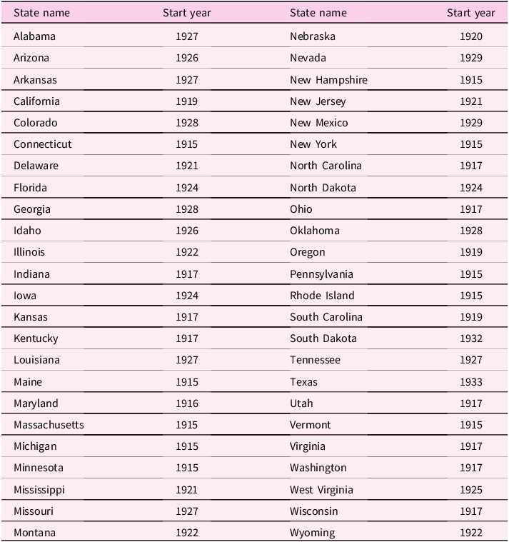
All counties and states did not start tracking live births at the same time. Table 1 lists the year that each state started reporting live births. Some states, such as Maine, report data going back to 1915, while others, such as Texas, only begin reporting live births during the 1930s. For all regressions, we limit ourselves to balanced panels of forty-six states that exclude both Texas and South Dakota. We combine the fertility dataset with data on state personal income per capita from 1919 to 1999 from Fishback and Kachanovskaya (Reference Fishback and Kachanovskaya2010). We use the consumer price index to transform all of the income data into real income using 1929 dollars. We lag income per capita by one year to account for the delay between conception decisions and observed births, so our income data span 1929 through 1940.
Date of fertility reporting

We also rely on data measuring key demographic differences across states and counties in 1920–log population, urbanization rates, marriage rates, age structure, female labor force participation rate, the percent of a locality that is female, as well as the percentage of a locality that is white. We use the IPUMS full sample for 1920 to calculate this demographic data (Ruggles et al., Reference Ruggles, Nelson, Sobek, Fitch, Goeken, Hacker, Roberts and Warren2024; Ruggles, et al., Reference Ruggles, Flood, Sobek, Backman, Cooper, Drew, Richards, Rodgers, Schroeder and Williams2025).
We measure uncertainty by following Chabe-Ferret and Gobbi (Reference Chabe-Ferret and Gobbi2018) and using the standard deviation in per capita income growth rates in the recent past. Thus, we are assuming that higher volatility in state economic growth is directly related to higher levels of uncertainty. Unlike Chabe-Ferret and Gobbi (Reference Chabe-Ferret and Gobbi2018), we do not measure “lifetime” volatility but instead measure a lagged volatility of growth rates over the previous three years for state s as shown below. $\overline {{g_{s,t}}} = {{1}\over{3}}\mathop \sum \nolimits_{i=0}^2 {g_{s,t - i}}$
where ${g_{s,t}}$
is the growth rate in per capita real income in state s between time t and t−1. Next, we estimate the standard deviation in growth for each state as shown below.
${g_{s,t}}$
is the growth rate in per capita real income in state s between time t and t−1. Next, we estimate the standard deviation in growth for each state as shown below. $Volatilit{y_{s,t}} = \;\sqrt {{{1}\over{2}}\mathop \sum \nolimits_{i=0}^2 {{\left( {{g_{s,t - i}} - \overline {{g_{s,t}}} } \right)}^2}}$
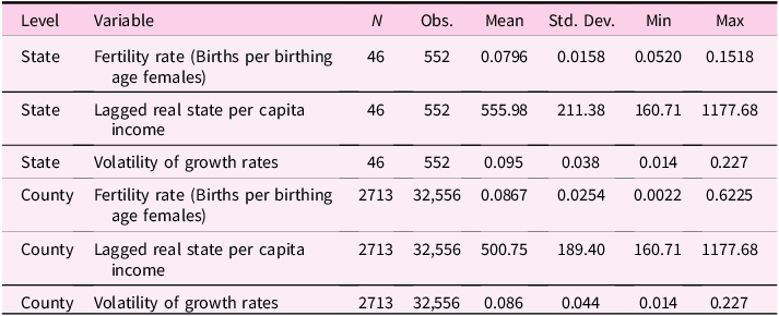
Table 2 presents summary statistics for fertility, lagged income, and growth volatility, along with the number of cross-sectional units and total observations.
Summary statistics

Notes: Real State Per Capita Income are in 1929 dollars and were converted using the consumer price index.
4. Empirical methodology
Our main equation of interest is $log \left( {Fertilit{y_{it}}} \right) = {\beta _1}log \left( {Incom{e_{s,t - 1}}} \right) + {\beta _2}\;Volatilit{y_{s,t}} + \Gamma X + \;{\varepsilon _{it}}$
where $Fertilit{y_{it}}$
measures the general fertility rate in place i at time t,
$Fertilit{y_{it}}$
measures the general fertility rate in place i at time t, $Incom{e_{st - 1}}$
measures the real income per capita in state s at time t-1 and
$Incom{e_{st - 1}}$
measures the real income per capita in state s at time t-1 and $Volatilit{y_{s,t}}$
measures the standard deviation in personal income in state s over the past three years.
$Volatilit{y_{s,t}}$
measures the standard deviation in personal income in state s over the past three years. ${\beta _1}$
estimates the elasticity of fertility with respect to per capita income. In order to interpret the coefficient on volatility, we standardize the volatility measure to have mean zero and a standard deviation of one. Thus, a one standard deviation increase in volatility is correlated with a
${\beta _1}$
estimates the elasticity of fertility with respect to per capita income. In order to interpret the coefficient on volatility, we standardize the volatility measure to have mean zero and a standard deviation of one. Thus, a one standard deviation increase in volatility is correlated with a $100 \cdot {\beta _2}$
percent change in fertility. X is a vector of various control variables and a constant with
$100 \cdot {\beta _2}$
percent change in fertility. X is a vector of various control variables and a constant with $\Gamma$
being a vector of coefficients corresponding to the controls.
$\Gamma$
being a vector of coefficients corresponding to the controls. $\varepsilon$
is the error term.
$\varepsilon$
is the error term.
When using county/state-level fertility data, we use county/state fixed effects to control for time-invariant unobserved heterogeneity across counties/states that may influence fertility rates. We also include year fixed effects to control for common time-varying factors that affect all counties/states simultaneously. Because long-run trends in per capita income and birthrates differ across localities, as a robustness check we control for state-specific linear time trends in order to isolate deviations in these series from local long-run secular changes.
We also believe it is important to control for important demographic variables – log population, urbanization rates, marriage rates, age structure, female labor force participation rate, the percent of a locality that is female, the percentage of a locality that is white, and the log of the locality’s infant mortality rate. Because most of these variables are only available during the years in which the population census was taken, we do not have annual data at either the state or county level. To address this issue, for most of these variables, we use their values in 1920 and interact them with year-fixed effects, allowing us to account for how their influence may change over time. The choice to use the 1920 values is made because we do not want any of the values of these variables to be determined by changes in income per capita or uncertainty over the course of the 1930s, which should help mitigate bias caused by including endogenous variables as control variables in the regression. The one variable that does not use the 1920 value is the log infant mortality rate due to a lack of data from all states in the sample. We instead use the 1930 value.
To interpret the regression coefficients causally, several key assumptions must be made. First, the model must satisfy the conditional exogeneity assumption, meaning that after controlling for the included covariates, the independent variables – log per capita income and volatility – are not correlated with unobserved determinants of fertility captured in the error term. This requires that no omitted variable bias remains, which is partially addressed through the inclusion of state and year fixed effects, state-specific linear time trends, and the demographic controls. Second, reverse causality must not drive the observed relationships, implying that changes in fertility do not systematically influence prior income, uncertainty, or volatility. The use of lagged income and uncertainty measures helps mitigate this concern.
For all regressions, we cluster our standard errors by state. Clustering at the state level allows for arbitrary correlation of the error terms within each state. Given that our independent variable of interest, personal income per capita, is measured at the state level, clustering at this level appropriately reflects the true variation in our estimates which prevents overstating the precision of our results. However, because we only have data on 46 states, the number of clusters is low enough to be concerned that the asymptotic properties of clustering do not hold. For all regressions presented in this paper, we compared the clustered standard errors with the normal non-robust standard errors as well as the robust White standard errors, and we find that the clustered standard errors reported in the tables are the more conservative ones.
5. Empirical results
5.1. Main results
Our main results are shown in Table 3. All columns use state-level fertility as the outcome of interest. Columns 1 through 5 do not include the volatility measure while columns 6 through 9 do. Column 1 presents a baseline specification with state fixed effects only. All subsequent columns include both state and year fixed effects. Columns 3 and 7 add linear state time trends and columns 4 and 8 include the full host of demographic time trends as described above in the methodology section. Finally, columns 5 and 9 include both the full host of demographic time trends as well as the linear state time trends.
Association between per capita income, volatility, and fertility rates

Notes: Dependent Variable is the log general fertility rate, as defined in the text. Sample is 46 states for 12 years from 1930 to 1941 (552 observations) for the dependent variable, fertility rates, while log real income per capita is lagged by one year (1929 to 1940). Growth volatility is defined in the text and is measured at the state level. Robust Standard Errors clustered by state are shown in parentheses. *p < 0.10, **p < 0.05, ***p < 0.01.
As can be seen, the elasticity of fertility rates with respect to lagged real income per capita, at the state level, ranges between 0.17 and 0.25 depending on the regression specification. The coefficients across all specifications are remarkably stable across all specifications, despite the progressive inclusion of stringent controls. Notably, the estimated coefficient in the most saturated specification, which includes both linear state trends and detailed demographic time trends, is nearly identical to that from the baseline specification with only state fixed effects. This similarity suggests that the more demanding specifications are not simply fitting noise. The specifications in columns 5 and 9 suggest that a 1 percent increase in real personal income last year is associated with roughly at 0.19 percent increase in fertility. All of our coefficients for lagged real income per capita are statistically significant at the 1 percent level. We do not weigh observations by state population in our reported results; however, doing so increases the estimated coefficient of lagged log of real income per capita across all specifications except for that in column 1, whereby the coefficient decreases slightly, although it remains statistically significant at the 1 percent level.
The specifications with state-specific linear trends are most comparable to Schaller et al., (Reference Schaller, Fishback and Marquardt2020), as those authors include state-specific linear trends in all specifications for their 1943–2016 sample. While they do not report results without these trends, our estimates with state-specific trends are similar to theirs. They estimate a coefficient of 0.209 compared to our estimates of 0.18 to 0.19 in comparable specifications. As they note, it is deviations from state-specific long-run secular changes in fertility and income that matter for the analysis.
In order to put these results into perspective, we estimate two counterfactual national birthrate time series. These counterfactuals estimate how fertility would have evolved during the 1930s in the absence of the steep declines in income per capita that occurred during the Great Depression. To estimate these counterfactual fertility paths for the 1930s, we use the coefficient on lagged income from our baseline regression, 0.189, to simulate how fertility would have evolved under an alternative income trajectory. Specifically, we adjust the observed fertility rate based on the difference between actual and counterfactual income, scaled by the estimated elasticity of fertility with respect to lagged income. The counterfactual fertility rate is constructed as: $log \left( {CF\;Fertilit{y_{it}}} \right) = log \left( {Fertilit{y_{it}}} \right) + {\hat \beta _1} \cdot \left[ {log \left( {CF\;Incom{e_{s,t - 1}}} \right) - log \left( {Incom{e_{s,t - 1}}} \right)} \right]$
The two counterfactual national birthrates come from our choice to use two counterfactual income trajectories. The first counterfactual assumes that each state’s income per capita during the 1930s remained at its 1929 level, essentially asking what fertility would have looked like if the Depression had frozen incomes rather than causing them to collapse. The second counterfactual assumes that the national growth rate in income per capita during the 1920s continued through the 1930s, representing a scenario where the prosperity of the Roaring Twenties extended uninterrupted into the following decade. Once we have our estimates for a counterfactual fertility rate in each state, we simply aggregate this fertility rate to the national level. Figure 1 plots the actual births per 1000 women aged 15 to 44 from 1925 to 1941 as well as the two counterfactual birthrates. Based on our counterfactual results, instead of bottoming out in 1933, the birthrate instead would have reached its minimum around 1937. The two counterfactuals suggest that there would have been roughly 5 to 6 additional births per every 1000 women aged 15 through 44 during 1933 and 1934, which would be roughly an 8 percent increase in the birthrate during the Great Depression. With a population of roughly 120 million in 1930, an additional 5 births per every 1000 women of birthing age for 5 years between 1931 and 1936 would imply that roughly 750,000 babies were not born due to the Great Depression.
Actual and counterfactual United States fertility rate 1925 to 1941.
Source: Historical Statistics of the United States Colonial Times to 1970, Part 1, Series B 5-10 “Birth Rate—Total and for Women 15-44 Years Old, by Race: 1800 to 1970.” as well as authors calculations. The data reports total live births per 1000 women aged 15 to 44.

Our estimated elasticities closely align with those reported by Schaller et al. (Reference Schaller, Fishback and Marquardt2020). Their findings suggest that the elasticity of fertility with respect to lagged state income per capita was approximately 0.15 during the period from 1974 to 2007 and around 0.21 over the broader timeframe of 1943 to 2007. The regression specification presented in column 3 of Table 3 most closely resembles their approach. Given this similarity and our estimated elasticity of roughly 0.18 for column 3 in Table 3, we find it reasonable to conclude that fertility patterns were likely just as procyclical during the Great Depression and New Deal era as they were in the post-World War II economy.
Table 3 also reports the R-squared for regression, the partial R-squared for the lagged log of real income per capita, and the residual variance share for the lagged log of real income per capita. The R-squared values indicate that our models explain between 89 percent and 99 percent of the total variation in fertility rates. These high R-squared values reflect the substantial explanatory power of state and year fixed effects, which capture persistent regional differences in fertility and common time trends across all states. The partial R-squared measures how much of the residual variation in fertility, after removing the contribution of all other controls and fixed effects, is explained by income. This statistic indicates how much income contributes to explaining fertility beyond what state and year fixed effects already capture. The partial R-squared estimates indicate that income explains between 4 percent and 14 percent of the residual variation in fertility after accounting for fixed effects and other controls. However, the partial R-squared does not directly measure effect sizes; the estimated coefficients themselves provide a more interpretable measure of the economic magnitude of the income-fertility relationship.
The residual variance share, calculated as (1−R2) from a regression of lagged income on the control variables, represents the proportion of the variation in income that remains after controls and fixed effects. The residual income variation ranges from 0.8 percent to 14 percent across specifications. Our most parsimonious specification with only state fixed effects (column 1) yields 14 percent residual variation share. Given substantial regional income disparities in the 1930s, it is unsurprising that state fixed effects alone explain the majority of income variation. A regression of log income on a single South dummy (former Confederate states) yields a residual variation share of approximately 60 percent, indicating this regional distinction alone explains approximately 40 percent of total variation. It is preferable to absorb this cross-sectional variation – which likely reflects persistent structural differences correlated with many unobserved factors – rather than relying on it for identification. Controlling for year fixed effects and various time trends further reduces the residual variance share. Despite this wide range in residual variance share, estimated coefficients for the income variable remain stable, varying only between 0.17 and 0.25. The stability of coefficients across specifications with such different residual variance shares suggests our results are not sensitive to the particular source of identifying variation after controlling for the cross-sectional differences in fertility and income across states. Moreover, even in our most demanding specifications, the standard deviation of residualized income remains economically meaningful, providing sufficient variation to estimate the income-fertility relationship with precision. The consistency of estimates across this range provides reassurance that we are capturing a robust economic relationship.
Motivated by recent work linking uncertainty to fertility behavior, we hypothesize that greater volatility in economic growth should depress fertility rates, all else equal. Surprisingly, we find null effects for volatility in some specifications and positive effects in other specifications. The positive coefficient found in column 7 of Table 3 suggests that a one standard deviation increase in volatility is associated with roughly an 0.8 percent increase in fertility. While statistically precise, the magnitude of this effect is economically small. Moreover, given the instability of the coefficient across specifications, we interpret this result cautiously and do not view it as robust evidence of a positive relationship.Footnote 3
These results are in direct contrast to recent research which has found that uncertainty causes decreases in fertility (Chabe-Ferret & Gobbi, Reference Chabe-Ferret and Gobbi2018). We note that our methodology measures the effect of past uncertainty and volatility on fertility decisions this year while Chabe-Ferret and Gobbi (Reference Chabe-Ferret and Gobbi2018) estimates the effect of total economic volatility a woman would experience between the ages of 21 and 35 on the decision to ever have a child. These two fertility decisions are quite different. It is possible that the relationship between uncertainty and fertility could be a positive one if when people were faced with greater uncertainty, individuals decide to invest in more of the “sure thing” of having kids rather than postponing kids until a date in an uncertain future.
5.2. Robustness checks
Fishback et al. (Reference Fishback, Haines and Kantor2007) examined the impact of government relief spending associated with President Franklin Roosevelt’s “New Deal” economic programs on births and deaths in the United States during the 1930s. They found that cities that received more New Deal spending had higher fertility rates, ceteris paribus, and they interpret their results as suggesting that New Deal relief spending encouraged couples to return to their normal fertility decisions and thus mitigated some of the potentially negative effects that the economic downturn otherwise had on fertility. Following Fishback et al. (Reference Fishback, Haines and Kantor2007) we employ New Deal spending as the sum of spending on four specific programs – the Civil Works Administration (CWA), the Federal Emergency Relief Administration (FERA), the Works Progress Administration (WPA), and the Social Security Administration (SSA).Footnote 4 The CWA operated only in 1933 and 1934, while the WPA and SSA began operation in 1935. FERA began spending after July 1, 1933, while the CWA operated only in the winter of 1933/1934 and its projects and workers then shifted to FERA. The WPA and SSA began expenditures in mid-1935. The state-level spending data on these four programs are for the fiscal years, which run July 1 to June 30. This makes them differ in timing of the other data in our analysis, which runs over the course of the calendar year. The spending data are all equal to zero prior to 1934 and are positive for each year from 1934 until the end of the decade.
Table 4 replicates our results shown in Table 3; however, we include the log of New Deal spending per capita as an additional control variable. Across all specifications, the coefficient on New Deal spending is positive and generally small. The largest coefficient suggests that a 1 percent increase in New Deal spending per capita increases the fertility rate by roughly 0.8 percent. Generally, as we include more time trends as controls, the coefficients on this variable become smaller and statistically insignificant. This suggests to us that inclusion of the time trends for the demographic variables likely overlap with key predictors of how policy makers decided to disperse New Deal funding over time. Still, the inclusion of New Deal spending only serves to increase the estimated elasticity between lagged real personal income per capita and fertility rates across all specifications.
Association between per capita income, volatility, and fertility rates, controlling for new deal spending

Notes: Dependent Variable is the log general fertility rate, as defined in the text. Sample is 46 states for 12 years from 1930 to 1941 (552 observations) for the dependent variable, fertility rate. Log real income per capita is lagged by one year (1929 to 1940). Growth volatility is defined in the text and is measured at the state level. Due to the inherent lagged nature of the federal government’s spending, new deal spending per capita is essentially also lagged (see the text for more information). Robust Standard Errors clustered by state are shown in parentheses. *p < 0.10, **p < 0.05, ***p < 0.01.
Recent research by Bellou et al. (Reference Bellou, Cardia and Lewis2025) finds that local economic shocks induced by the Great Depression, measured by changes in retail sales per capita, led to immediate declines in fertility at the county level, followed by substantial fertility increases approximately two decades later. To ensure parallel pre-trends in their estimation, they analyze the dynamic effects of retail sales per capita while controlling for state-by-year fixed effects. While the Great Depression’s impact varied significantly across counties within states, considerable heterogeneity also existed in the severity of the downturn across states, along with economic disruptions not fully captured by retail sales. Schaller et al. (Reference Schaller, Fishback and Marquardt2020) estimate the relationship between per capita income and fertility using both county- and state-level income measures, demonstrating that both localized and broader regional economic shocks play a significant role in shaping fertility decisions.
Table 5 presents results in which we interact the percentage change in retail sales per capita between 1929 and 1933 with year fixed effects, allowing us to estimate the dynamic effects of the Great Depression as captured by this economic measure. Unlike Bellou et al. (Reference Bellou, Cardia and Lewis2025), we do not include state-by-year fixed effects, which enables us to assess the impact of lagged real income per capita at the state level on fertility rates. However, our inclusion of linear state time trends is motivated by similar concerns that led them to adopt state-by-year fixed effects. Additionally, Table 5 incorporates the log of New Deal spending per capita at the state level. While we do not explicitly report the dynamic effects of retail sales per capita on fertility, our estimated coefficients align closely with those presented in Bellou et al. (Reference Bellou, Cardia and Lewis2025). Importantly, even after accounting for this Great Depression shock, the estimated elasticity of fertility with respect to lagged state personal income per capita remains positive and statistically significant. The coefficients are slightly attenuated compared to those in Tables 3 and 4, likely due to the dynamic effect of the percent change in retail sales per capita between 1929 and 1933 capturing variation in both fertility and state-level personal income per capita during this period. Overall, these findings underscore the importance of both localized and broader state-level economic conditions in influencing fertility behavior.
Association between per capita income, volatility, and fertility rates, controlling for new deal spending and retail sales shock

Notes: Dependent Variable is the log general fertility rate, as defined in the text. Sample is 46 states for 12 years from 1930 to 1941 (552 observations) for the dependent variable, fertility rate. Log real income per capita is lagged by one year (1929 to 1940). Growth volatility is defined in the text and is measured at the state level. Due to the inherent lagged nature of the federal government’s spending, new deal spending per capita is essentially also lagged (see the text for more information). Robust Standard Errors clustered by state are shown in parentheses. *p < 0.10, **p < 0.05, ***p < 0.01.
5.3. County-level results
The Bailey et al. (Reference Bailey, Clay, Fishback, Haines, Kantor, Severnini and Wentz2016) dataset contains the county-level fertility that we aggregated to the state level in the previous sections of the paper. As an additional robustness check, we estimate the association of lagged income per capita at the state level on county-level fertility rates. We opted to include both the retail sales shock time trends and the New Deal spending control variable. We weight the observations by the population in each county in 1930 since the main control variables of interest vary only at the state level. If each county is given equal weight, the regression may disproportionately reflect the characteristics of smaller counties rather than reflecting the population distribution within each state. Weighting by population ensures that the regression reflects the average experience of individuals, not just counties. Results are shown in Table 6 and show results similar to those of the state-level regressions, although the estimated elasticity in columns 4 and 8 are around half the magnitude of the elasticities estimated at the state level in Table 5. Still, these results still tell the same overall story suggested by the main results.
Association between per capita income, volatility, and fertility rates using county-level data, controlling for new deal spending and retail sales shock

Notes: Dependent Variable is the log general fertility rate at the county level, as defined in the text. Sample is 2713 counties for 12 years from 1930 to 1941 (32,556 observations). Log real income per capita is lagged by one year (1929 to 1940) and is measure at the state level. Growth volatility is defined in the text and is measured at the state level. Due to the inherent lagged nature of the federal government’s spending, new deal spending per capita is essentially also lagged (see the text for more information) and is also measured at the state level. Observations are weighted by the county population in 1930. Robust Standard Errors clustered by state are shown in parentheses. *p < 0.10, **p < 0.05, ***p < 0.01.
5.4. Dynamic effects
Finally, we estimate the dynamic effects of state per capita income on fertility decisions using the following distributed lag model: $log \left( {Fertilit{y_{it}}} \right) = \mathop \sum \limits_{\tau =0}^7 {\beta _\tau }log \left( {Incom{e_{s,t - \tau }}} \right) + {\Gamma} X + \;{\varepsilon _{it}}$
where ${\beta _\tau }$
estimates the elasticity of state per capita income
${\beta _\tau }$
estimates the elasticity of state per capita income $\tau$
years in the past on fertility rates this year. The inclusion of lagged income terms requires extending our income data back to 1923 in order to avoid truncating the sample. This dynamic regression analyzes the influence of economic shocks on birth rates, both in the present and over time, through delayed effects and changes in timing, such as postponement or harvesting.
$\tau$
years in the past on fertility rates this year. The inclusion of lagged income terms requires extending our income data back to 1923 in order to avoid truncating the sample. This dynamic regression analyzes the influence of economic shocks on birth rates, both in the present and over time, through delayed effects and changes in timing, such as postponement or harvesting.
Figure 2 plots the ${\beta _\tau }$
coefficients when controlling for state fixed effects, year fixed effects, linear state time trends, and demographic time trends using state-level fertility data as the output table. The results suggest that the cumulative effects of a positive income shock are increasing for only two years before becoming statistically insignificant. This is in contrast with both Schaller et al. (Reference Schaller, Fishback and Marquardt2020) and Currie and Schwandt (Reference Currie and Schwandt2014) who both find longer-lasting dynamic effects on fertility.
${\beta _\tau }$
coefficients when controlling for state fixed effects, year fixed effects, linear state time trends, and demographic time trends using state-level fertility data as the output table. The results suggest that the cumulative effects of a positive income shock are increasing for only two years before becoming statistically insignificant. This is in contrast with both Schaller et al. (Reference Schaller, Fishback and Marquardt2020) and Currie and Schwandt (Reference Currie and Schwandt2014) who both find longer-lasting dynamic effects on fertility.
Dynamic effects of state income per capita on fertility.
Notes: This figure plots coefficient estimates for the dynamic effect of state per capita income on fertility decisions using the distributed lag model described in the text.

There are multiple possible explanations for why the effects of an income shock are not as long-lasting in our sample. First, our shorter sample period may limit our ability to detect longer-lasting dynamic effects. Second, economic conditions, policy environments, and access to family planning have changed markedly over time, potentially influencing how quickly fertility responds to income fluctuations. For example, in the earlier period that we study, birth control was less widespread, and social norms around family size may have been less elastic in response to short-run economic changes, potentially leading to more muted or short-lived responses.
6. Conclusion
Our analysis demonstrates that United States’ fertility patterns during the Great Depression were procyclical, with elasticities – generally between 0.17 and 0.25 – that were remarkably similar to those observed in the post-World War II era. In short, ceteris partibus, those states that were hit hardest by the economic effects of the Great Depression saw a larger negative impact on fertility than those affected less. Counterfactual estimates suggest that the economic hardship of the 1930s resulted in roughly 750,000 fewer births nationwide. Our results are robust across various specifications, including controls for state-specific linear time trends, time trends for a host of demographic variables, New Deal spending, and when controlling for the dynamic effects of the percent change in retail sales between 1929 and 1933. Our findings are consistent with papers showing how birth rates were negatively impacted by Great Recession of 2008 across much of the world. The similarity between our estimated elasticities and those found in more recent periods suggests that the relationship between economic conditions and US fertility decisions has remained relatively stable over nearly a century, despite substantial changes in social norms, female labor force participation, and contraceptive technology.
Interestingly, and in contrast to recent literature examining more contemporary periods, we find no evidence that economic uncertainty negatively impacted US fertility decisions during the Great Depression. Our income volatility measure shows null or slightly positive effects on fertility rates, suggesting that the mechanisms linking economic uncertainty to fertility decisions may have evolved over time. The dynamic effects of income shocks on fertility appear more muted during our sample period compared to post-World War II estimates, with significant effects lasting only two years.


 Open access