


Introduction
Due to climate change, glaciers are expected to lose a substantial fraction of their volume in the coming decades (Marzeion and others, Reference Marzeion, Jarosch and Hofer2012; Radić and Hock, Reference Radić and Hock2014; Huss and Hock, Reference Huss and Hock2015; Kraaijenbrink and others, Reference Kraaijenbrink, Bierkens, Lutz and Immerzeel2017; Hock and others, Reference Hock2019; Marzeion and others, Reference Marzeion2020; Rounce and others, Reference Rounce, Hock and Shean2020a). Even though glaciers contain <1% of the ice volume on Earth (here we use the term ‘glaciers’ to refer to all land ice masses separated from the Greenland and Antarctic ice sheets), their mass loss has been estimated to be a major contributor to 20th century sea-level rise (IPCC, Reference IPCC2019). Moreover, their retreat is anticipated to have severe impacts on water availability (e.g. Kaser and others, Reference Kaser, Grosshauser and Marzeion2010; Huss and Hock, Reference Huss and Hock2018; Pritchard, Reference Pritchard2019), hydropower production (e.g. Farinotti and others, Reference Farinotti, Round, Huss, Compagno and Zekollari2019b; Schaefli and others, Reference Schaefli, Manso, Fischer, Huss and Farinotti2019), natural hazards (e.g. Gilbert and others, Reference Gilbert, Vincent, Gagliardini, Krug and Berthier2015; Kääb and others, Reference Kääb2018), and tourism (e.g. Fischer and others, Reference Fischer, Olefs and Abermann2011; Stewart and others, Reference Stewart2016; Tórhallsdóttir and Ólafsson, Reference Tórhallsdóttir and Ólafsson2017).
The future evolution of individual Scandinavian and Icelandic glaciers has been the focus of a number of local studies, including studies in which the ice flow is treated by flowline models (e.g. Oerlemans, Reference Oerlemans1997; Laumann and Nesje, Reference Laumann and Nesje2009a, Reference Laumann and Nesje2009b), two-dimensional (2-D) (vertically integrated) models (e.g. Flowers and others, Reference Flowers, Marshall, Björnsson and Clarke2005; Marshall, Reference Marshall2005; Aðalgeirsdóttir and others, Reference Aðalgeirsdóttir, Jóhannesson, Björnsson, Pálsson and Sigurðsson2006; Andreassen and Oerlemans, Reference Andreassen and Oerlemans2009; Aðalgeirsdóttir and others, Reference Guðmundsson2009; Giesen and Oerlemans, Reference Giesen and Oerlemans2010; Aðalgeirsdóttir and others, Reference Aðalgeirsdóttir2011; Laumann and Nesje, Reference Laumann and Nesje2014; Åkesson and others, Reference Åkesson, Nisancioglu, Giesen and Morlighem2017) or 3-D models (e.g. Schmidt and others, Reference Schmidt2020). Whilst all of these studies agree that glaciers will lose a significant part of their volume in the future, the glacier-specific characteristics determining glacier evolution mean that the findings cannot easily be extrapolated to region-wide projections of glacier changes.
For Scandinavia and Iceland, global-scale models with varying degrees of complexity (e.g. Raper and Braithwaite, Reference Raper and Braithwaite2006; Radić and Hock, Reference Radić and Hock2011; Marzeion and others, Reference Marzeion, Jarosch and Hofer2012; Slangen and others, Reference Slangen, Katsman, van de Wal, Vermeersen and Riva2012; Giesen and Oerlemans, Reference Giesen and Oerlemans2013; Hirabayashi and others, Reference Hirabayashi, Zang, Watanabe, Koirala and Kanae2013; Radić and Hock, Reference Radić and Hock2014; Huss and Hock, Reference Huss and Hock2015; Hock and others, Reference Hock2019; Marzeion and others, Reference Marzeion2020) have been used. Most global-scale glacier models, however, do not explicitly account for the effects of ice-flow dynamics or glacier geometry, and none of the related studies calibrated the glaciers’ mass balance with glacier-specific data so far. Similarly, large-scale studies that account for ice dynamics using the Shallow Ice Approximation (SIA) (Hutter, Reference Hutter1983) now exist (Clarke and others, Reference Clarke, Jarosch, Anslow, Radić and Menounos2015; Maussion and others, Reference Maussion2019; Zekollari and others, Reference Zekollari, Huss and Farinotti2019), but the future evolution of Scandinavian and Icelandic glaciers was never addressed with such a framework. Although recognising that flowline-based models might fail to capture some important dynamics for ice caps, e.g such as the temporal migration of ice divides, such simplified approaches are still necessary for regional-scale studies.
Future glacier evolution is strongly governed by the surface mass balance, which is driven by climatic conditions. Climate forcing products, comprising both past climate data products (E-OBS, ERA-I and ERA-5) and future climate projections (RCMs and GCMs), are evolving continuously by offering an increasing spatial resolution or by taking advantage of improved assimilation methods and enhanced parametrisations (Jacob and others, Reference Jacob2014; Stouffer and others, Reference Stouffer2017; Sørland and others, Reference Sørland, Schär, Lüthi and Kjellström2018; Hersbach and others, Reference Hersbach2019). Most often, global glacier modelling studies aim at using the most up-to-date climate forcing product of their time. This makes individual studies differ in terms of climate forcing, which makes it difficult to directly compare the results of individual models (Hock and others, Reference Hock2019). And since glacier evolution is directly driven by climate, it is crucial to know how various climate forcing products affect modelled glacier response. In this paper, we model the future evolution of all Scandinavian and Icelandic glaciers (Fig. 1) using the Global Glacier Evolution Model with an ice-flow component (GloGEMflow, Zekollari and others, Reference Zekollari, Huss and Farinotti2019), introduce a new glacier-specific geometry initialisation procedure, and quantify the effect that different climate forcing products have on the modelled glacier evolution. The surface mass-balance model is calibrated with observations of glacier-specific geodetic ice volume changes (Zemp and others, Reference Zemp2019), and the results are validated agains an extensive set of independent data including ice-flow velocities retrieved from remote sensing (Gardner and others, Reference Gardner, Fahnestock and Scambos2019; Nagy and Andreassen, Reference Nagy and Andreassen2019), length-change observations (WGMS, Reference WGMS2019) and in-situ mass balances that were acquired with the glaciological method (WGMS, Reference WGMS2019).
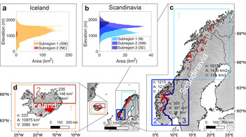
(a, b) Glacier hypsometry at the inventory date (RGI Consortium, Reference RGI Consortium2017) for Iceland and Scandinavia, where each colour represents a subregion. (c, d) Extent of Scandinavian and Icelandic glaciers (red), typically between 1999 and 2006. The orange and blue squares show the subregions considered in the study. For each subregion, n is the total number of glacier entities comprised in the RGI6.0, A is the total glacier area and V is the total glacier ice volume according to Farinotti and others (Reference Farinotti2019a). Note that especially for Iceland, the number of glaciers is increased by the subdivision of ice caps into single glaciers (RGI Consortium, Reference RGI Consortium2017). Map source: Natural Earth.

Although ca. 95 % of the ice volume in Iceland is found in ice caps, which would be better treated by explicit 3D modelling, Scandinavia and Iceland are chosen because extensive observational data document their recent glacier changes, the two regions have substantially different glacier characteristics (i.e. glacier volume, area, ice thickness etc.; see Fig. 1), and the share of debris-covered glaciers is small (3.4% for Scandinavian and 2.9% for Icelandic glaciers, Scherler and others, Reference Scherler, Wulf and Gorelick2018). The latter simplifies the relation between climate forcing and glacier response (Kraaijenbrink and others, Reference Kraaijenbrink, Bierkens, Lutz and Immerzeel2017), making the results easier to interpret. Furthermore, detailed climate forcing products exist for both past and future. A gridded observational data set (E-OBS) as well as an ensemble of high-resolution regional climate models (RCMs) simulations (EURO-CORDEX) exist for the two regions, thus providing the means of a detailed assessment of their influece. More specifically, we consider E-OBS and two re-analysis products (ERA-I and ERA-5) for the period 1979–2018 (1950–2018 for E-OBS), and use both high-resolution RCM from EURO-CORDEX (Jacob and others, Reference Jacob2014) and global circulation models (GCMs) included in the Coupled Model Intercomparison Project (CMIP5) for the period 2018–2100. These climate forcing products are consistent with what was used in several large-scale glacier-evolution studies (e.g. Anderson and Mackintosh, Reference Anderson and Mackintosh2012; Giesen and Oerlemans, Reference Giesen and Oerlemans2013; Radić and others, Reference Radić2014; Huss and Hock, Reference Huss and Hock2015; Kraaijenbrink and others, Reference Kraaijenbrink, Bierkens, Lutz and Immerzeel2017; Sakai and Fujita, Reference Sakai and Fujita2017; Farinotti and others, Reference Farinotti, Round, Huss, Compagno and Zekollari2019b; Schaefli and others, Reference Schaefli, Manso, Fischer, Huss and Farinotti2019; Zekollari and others, Reference Zekollari, Huss and Farinotti2019; Marzeion and others, Reference Marzeion2020; Rounce and others, Reference Rounce, Hock and Shean2020a), thus allowing for our results to be compared. The ensemble of products also allows us to assess the differences in modelled future glacier evolution caused by the choice of climate product versions (ERA-5 versus ERA-I) and origins (observational versus reanalysis data).
Data
Our study focuses on all 3411 glaciers in Scandinavia (3143 in Norway and 268 in Sweden) and all 568 glaciers in Iceland included in the Randolph Glacier Inventory version 6 (RGI 6.0; RGI Consortium, 2017, Fig. 1). The RGI is a globally complete inventory of glacier outlines, typically dating from the early 21st century (1999–2006 for Scandinavia, and 1999–2004 for Iceland; see Table S1). For Scandinavia, those data are taken from various regional sources (e.g. Andreassen and others, Reference Andreassen, Paul, Kääb and Hausberg2008; Paul and Andreassen, Reference Paul and Andreassen2009; Paul and others, Reference Paul, Andreassen and Winsvold2011). All three studies used Landsat Thematic Mapper scenes but refer to different points in time and different regions: Andreassen and others (Reference Andreassen, Paul, Kääb and Hausberg2008) used a scene from 2003 to map 417 glaciers in the Jotunheimen and Breheimen regions (Southern Norway); Paul and Andreassen (Reference Paul and Andreassen2009) used scenes from 1999 to map 489 glaciers in the Svartisen region (Northern Norway); and Paul and others (Reference Paul, Andreassen and Winsvold2011) used a scene from 2006 to map 1450 glaciers in the Jostedalsbreen region (Southern Norway). For Iceland, majority of the outlines were extracted from 1999–2004 ASTER and SPOT5 imagery (Sigurðsson and others, Reference Sigurðsson, Williams, Martinis and Münzer2014).
The glacier ice thickness distribution is derived from the consensus estimate by Farinotti and others (Reference Farinotti2019a), which is a multi-model ensemble providing estimates for all glaciers within the RGI 6.0. For each glacier, both the glacier geometry and the ice thickness are aggregated to surface elevation bands of 10 m (Huss and Hock, Reference Huss and Hock2015). All tributary glaciers are included in a given elevation band, i.e. they are not treated separately.
For forcing the model in the past (1950–2018 for E-OBS; 1979–2018 for ERA), we use monthly 2-m air temperature and total precipitation from (i) the ensemble daily gridded observational dataset (E-OBS) v.19.0 (Cornes and others, Reference Cornes, van der Schrier, van den Besselaar and Jones2018), (ii) the European Centre for Medium-Range Weather Forecasts Interim re-analysis (ERA-Interim, hereafter referred to as ERA-I) (Dee and others, Reference Dee2011) and (iii) ERA-5 (Hersbach and others, Reference Hersbach2019). The three climate data products for the past (Fig. 2) have a different time coverage and spatial resolution, as given in Table 1. For the future (2018–2100), we use monthly outputs from both CMIP5 GCMs (70 model members), and EURO-CORDEX RCMs (51 model members) (Jacob and others, Reference Jacob2014; Kotlarski and others, Reference Kotlarski2014, Table I). GCM and RCM simulations are driven with different Representative Concentration Pathways (RCP2.6, RCP4.5 and RCP8.5). RCP2.6 is a scenario implying stringent greenhouse gas mitigation, RCP8.5 is a scenario without reduction of greenhouse gas emissions, and RCP4.5 is an intermediate scenario (IPCC, Reference IPCC2013). We modelled all glaciers based on 70 GCMs, 51 RCMs and for three climate data products each, i.e. the evolution of every glacier was simulated 363 times.
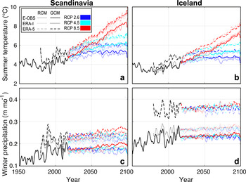
(a, b) Average summer (1 May–30 September) air temperature and (c, d) winter (1 October– 30 April) precipitation. Panels a and c refer to Scandinavia, panels b and d refer to Iceland. The values are weighted averages of the climate re-analysis grid cell values, the weight being given by the number of glaciers larger than 1 km2 within every grid cell. Series are smoothed with a 2-year running mean. The line type (solid, dotted, dashed) shows the past climate data products (E-OBS, ERA-I, ERA-5; see Methods section). The change in variability between past and future is the result of averaging all RCM and GCM members.

Climate forcing products used in this study

The GCMs have different spatial resolutions. ‘cov.’ stands for ‘coverage’. ‘Members’ indicates the number of model realisations per data set.
To merge the past and future monthly series of air temperature and precipitation, a de-biasing scheme is applied (Huss and Hock, Reference Huss and Hock2015). The scheme aims at avoiding sudden change between past climate data products (E-OBS, ERA-I and ERA-5) and future climate projections (GCM, RCM), and ensures consistency of the climatic forcing over time. In the first step, the additive (temperature) and multiplicative (precipitation) monthly biases between the past and future climate projections are calculated over the time period 1980–2010, which is the period covered by both past climate products and future projections. These biases are then superimposed on the future climate projections, thus assuming the biases to remain constant in time. In the second step, consistency in the interannual variability of temperature is ensured. This is done in a two-step procedure. First, the standard deviation of the time series is calculated for each month (m) of both the past climate product (σp,m) and the future climate projection (σf,m). Note that also the future climate projections have data of the past. Then, the interannual temperature variability of the future climate projection T m,t is corrected as:

where $\overline {T_{m, 25}}$ is the mean temperature in a 25-year period around t (see (Huss and Hock, Reference Huss and Hock2015), for more details). This procedure yields a continuous and homogeneous time-series spanning from 1950/79 to 2100. By applying this approach whilst using the high spatial resolution offered by the past climate products as reference, moreover, the GCMs are downscaled to this finer horizontal resolution. In particular, the information on small-scale spatial climate variability provided by the past climate products is transferred to the GCMs.
For model calibration, we rely on a comprehensive data set of geodetic mass balances that cover both the Scandinavian and Icelandic glaciers (Zemp and others, Reference Zemp2019). We rely on all entries provided by the World Glacier Monitoring Service (WGMS) data base (WGMS, Reference WGMS2019), which is a collection of worldwide mass-balance observations. The database was substantially expanded recently, when >10,000 glacier-specific elevation change measurements for Scandinavia and Iceland were included. These measurements often include multiple time periods per glacier, and are derived from photogrammetrical evaluation of Advanced Spaceborne Thermal Emission and Reflection Radiometer (ASTER) imagery (Girod and others, Reference Girod, Nuth, Kääb, McNabb and Galland2017; Zemp and others, Reference Zemp2019). When multiple geodetic mass change estimates are available for the same glacier, the information on annual mass-balance variability provided from glaciological observations is used to align the estimates during the period 2003–2014 (i.e. the period covered by most observations) and the estimates are then averaged (see Zemp and others, Reference Zemp2019, for details). This allows to obtain geodetic volume changes for 70% (2064 km2) of the total glacier area of Scandinavia and 79% (8737 km2) of the total glacier area of Iceland. For glaciers with no observations, data from a nearby glacier is chosen. This is done by selecting the glacier that minimises the metric P = d*(ΔA)/A 0, where d is the horizontal distance between the two glaciers (in km), ΔA is the difference in area between the two glaciers and A 0 is the area (in km2) of the glacier with no observation (Zekollari and others, Reference Zekollari, Huss and Farinotti2019). This approach aims at accounting for both climate patterns (by considering the distance between glaciers) and glacier characteristics (by considering the glacier area).
Methods
GloGEMflow is a combined mass-balance and ice-flow model. In the first step, the mass balance of each glacier is calculated (Huss and Hock, Reference Huss and Hock2015). In the second step, the glacier's ice flow is modelled with a 1-D model (details follow below). The glacier geometry is divided into elevation bands, where the glacier cross-section within each elevation band is parameterised by using an isoscele trapezoid with 45° base angles (see Zekollari and others, Reference Zekollari, Huss and Farinotti2019, for details). The limited influence of the base angles on the glacier evolution was shown in the same publication, whilst a discussion of the applicability of the assumption to ice caps follows in discussion section.
Mass-balance model
In the surface mass-balance model, accumulation is determined by solid precipitation, which is distinguished from liquid precipitation based on the temperature: all precipitation occurring at the temperatures below 0.5°C (above 2.5°C) is considered to be solid (liquid), with a linear transition in between. The precipitation given by the input climate forcing product for the grid cell closest to the glacier is distributed across the glacier surface with a rate of 1.5% for each 100 m of elevation gain. This elevation gradient is chosen such as to maximise the agreement with the WGMS accumulation data (WGMS, Reference WGMS2019). Ablation is computed by using a temperature-index melt model (Hock, Reference Hock2003) and assuming that melt occurs at days where temperature is above 0 °C. Ice, firn and snow are discerned by using different degree-day factors (DDFs), with a ratio of 2 between the DDF for ice and the DDF for snow, and a ratio of 1.5 between the DDF for ice and the DDF for firn (see Discussion for an analysis of these ratios). For E-OBS, which provides 2-m air temperature, the temperature lapse rate is determined from the relation between temperature and elevation for all grid cells within a radius of 50 km of the glacier. For ERA-I and ERA-5, providing monthly temperature fields at various geopotential heights, the temperature lapse rate is obtained by determining the average rate of temperature change with elevation for each grid cell. In both cases, the lapse rates are derived at a monthly resolution (i.e. at the time resolution of the past climate product), and are kept constant to ensure consistency when transitioning from past to future climatic conditions. For Scandinavia, the procedure results in yearly mean lapse rates of −0.59 ± 0.09, −0.54 ± 0.04 and −0.54 ± 0.04°C (100 m)−1 for E-OBS, ERA-I and ERA-5, respectively. For Iceland, the corresponding lapse rates are of −0.62 ± 0.08, −0.57 ± 0.04 and −0.56 ± 0.03°C (100 m)−1. Refreezing of melt water and liquid precipitation in the first 10 m of snow/firn/ice below the surface is computed based on temperatures of the sub-surface as estimated from heat conduction (see Huss and Hock, Reference Huss and Hock2015, for details). However, the refreezing contribution to overall accumulation is very small (<1% for both regions). Following Huss and Hock (Reference Huss and Hock2015), frontal ablation of glaciers with bedrock elevation below sea-level glaciers is accounted for by adopting an adapted version of the approach by Oerlemans and Nick (Reference Oerlemans and Nick2005). Frontal ablation is modelled as a function of the water depth, the slope of the glacier within 100 m of elevation from the calving front, and the height and width of the calving front (see Huss and Hock, Reference Huss and Hock2015, for more details). Frontal ablation of lake-terminating glaciers (i.e. above the sea level) was not accounted for, due to uncertainties related to existing and future lake geometries. Note that among all the glaciers that were modelled in this study, only seven Icelandic glaciers have bedrock elevations reaching below present-day sea level. Therefore, frontal ablation was only modelled for these seven glaciers. For the period 1990–2020, we estimate that frontal ablation contributed to ~3.5% of the total ablation of these glaciers (see Fig. S2). In the near future (2025–50), this rate is anticipated to locally increase to up to 20%. This is due to the retrograde bedrock slopes that cause increasing water depths at the calving fronts as glaciers retreat further. After ~2050, however, the glaciers will have retreated out of the deepest bedrock sections, thus resulting in a reduction and, eventually, cessation of calving. This temporal evolution is consistent with results obtained from local studies (Björnsson and others, Reference Björnsson, Pálsson and Guðmundsson2001; Jóhannesson and others, Reference Jóhannesson2020).
To account for the actual sensitivity of each glacier to climate (Rounce and others, Reference Rounce2020b), a glacier-specific calibration of the mass-balance model is needed (Fig. 3). For each glacier, the precipitation correction factor (first step), the degree-day factor (second step) and the air temperature (third step) are adjusted, until the difference between modelled and observed geodetic mass balance is within ±0.1 m w.e. a−1 (see Fig. 3). The second and the third steps, respectively, are only required when no agreement is found during the first step. In the first step, the precipitation is multiplied by an enhancement factor, which is varied between 0.8 and 2.0 for Scandinavia, and between 1.8 and 3.0 for Iceland (for consistency, the same factors as in Huss and Hock, Reference Huss and Hock2015, were used). This factor is meant to account for the local-scale precipitation patterns that are not captured by the climate forcing products, as well as for snow drift and avalanches (e.g. Machguth and others, Reference Machguth, Eisen, Paul and Hoelzle2006; Helfricht and others, Reference Helfricht, Lehning, Sailer and Kuhn2015). For each glacier, the precipitation enhancement factor is chosen to minimise the misfit with annual mass balance over the period covered by geodetic surveys. In this case, the DDF snow is generally set to 3 mm w.e. d−1 K−1. If the misfit exceeds the ±0.1 m w.e. a−1 threshold, the precipitation enhancement factor is fixed at either the maximum or the minimum of the permitted range and, in the second step, DDF snow is adjusted to minimise the misfit. To do so, DDF snow is varied between 1.75 and 4.50 mm d−1 K−1, corresponding to the literature values Hock (Reference Hock2003). If at this stage the difference between modelled and observed mass balance is still larger than ±0.1 m w.e. a−1, the mass balance at the glacier-site cannot be modelled with a realistic parameter range. This indicates a bias in the local or regional climatic conditions, i.e. that the latter are inconsistent with the observed glacier changes. Hence, the third step adjusts the temperature until an agreement between observed and modelled glacier mass balance is reached. The results of this glacier-specific calibration are summarised in Supplementary Table S2.
Mass-balance model calibration procedure for every glacier. The procedure is divided into three steps, and is completed when the modelled and observed geodetic mass balance agree within a given threshold (e = ±0.1 m w.e. a−1) which is checked after every step. ‘MB’ stands for mass balance.

Ice-flow model
We model ice flow explicitly for all glaciers with an area larger than 1 km2 in the RGI. This corresponds to 93.4 and 99.9% of the ice volume for the Scandinavian and Icelandic glaciers, respectively. For the remaining glaciers, the geometry evolution is modelled using the Δh parameterisation (Huss and others, Reference Huss, Jouvet, Farinotti and Bauder2010), in which local ice thickness changes are imposed based on an elevation-dependent parameterisation (this corresponds to the original version of GloGEM by Huss and Hock, Reference Huss and Hock2015). We thus assume that ice flow plays only a secondary role for the geometry evolution of glaciers smaller than 1 km2.
For glaciers larger than 1 km2 ice flow is modelled by applying the Shallow-Ice Approximation (SIA) (Hutter, Reference Hutter1983) along the previously-defined elevation bands (see Data section). Ice flux is expressed through a diffusivity equation whilst the continuity equation for ice thickness is used to calculate the glaciers’ temporal evolution. The model has been described in detail in Zekollari and others (Reference Zekollari, Huss and Farinotti2019), where details on time stepping, spatial discretisation, and model implementation can be found. Using this method, the ice flow depends on a deformation-sliding factor, which accounts for both ice deformation and basal sliding (again, see Zekollari and others, Reference Zekollari, Huss and Farinotti2019, for details). We thus follow the method of Zekollari and others (Reference Zekollari, Huss and Farinotti2019) in which the components are treated together. The argument is that both deformation and sliding are strongly linked to the local ice thickness and surface slope, thus resulting in similar spatial patterns (e.g. Zekollari and others, Reference Zekollari, Huybrechts, Fürst, Rybak and Eisen2013). The same approach has been used in various studies (e.g. Gudmundsson, Reference Gudmundsson1999; Clarke and others, Reference Clarke, Jarosch, Anslow, Radić and Menounos2015).
To initialise the model, an iterative procedure is used to generate a glacier-specific, transient state referring to the glaciers’ inventory date. In the procedure, the model is first forced with a constant climate until the glacier reaches a steady-state geometry. The constant climate corresponds to a mean climate over a time period Δt s, which is chosen for the cumulative glacier mass balance over this period to be close to zero (see text in Supplementary Material S1 for the details of this procedure). For this period, the glacier mass balance is computed using the calibrated mass-balance model. After that, starting from this initial steady-state geometry, a transient simulation with EOBS, ERA-I or ERA-5 data is performed for half of the glacier's response time (t s) from t i − t s/2 on until t i, where t i is the date of the glacier inventory for the glacier (see Fig. S1). After that, resulting glacier volume and length are compared to observations. In order to match the glacier volume and length at the inventory date, the deformation-sliding factor and the geometry of the initial steady-state glacier are modified, respectively. The geometry of the initial steady state is modified by adding a mass-balance bias on the top of the constant climate which is used to reach a steady-state geometry (through an ELA perturbation). As the time interval between the steady-state geometry and the transient geometry is relatively limited (corresponding to half of the glacier response time), the steady-state geometry directly affects the geometry at the inventory date (and its length). This two-step calibration procedure is repeated iteratively until the observations are matched (difference below 1%). Supplementary Chapter S1 offers more details on this initialisation procedure.
Evaluation of model performance
The model performance is evaluated against a comprehensive set of independent data, including surface mass balances (seasonal glacier-wide observations and measurements specified for elevation bands), glacier length changes, as well as in-situ and satellite-based observations of the surface flow speed. As performance metrics, we use the bias (i.e. the difference between observations and modelled results), the root-mean-square error (RMSE), the coefficients of determination (r 2) and the mean absolute deviation divided by the standard deviation. The latter (we call it MASD) is a relative metric providing information on how the average model misfit compares against the typical variability of the observational data. A MASD value of ‘1’, thus, indicates that the average misfit is as large as the data's intrinsic variability. If not stated otherwise, the values provided in the following subsections and in Table 2 refer to an average over all glaciers and over the three past climate data products (E-OBS, ERA-I, ERA-5) that are used to drive the model simulations in the past.
Evaluation of model performance against various observations including surface mass balance, length changes and ice-flow velocity

For every data set, the number of samples n, the bias, the RMSE, r 2 and the MASD is given. The bias is computed as the average difference between observations and model results. B a and B w are annual and winter glacier-wide surface mass balances, respectively. For Iceland, no information on elevation band surface mass balance is available. ‘Max velocity diff.’ compares the 99% quantile of the observed and modelled velocities. ‘MB’ stands for the mass balance. The ranking is used to determine which of the past climate data products results in the best agreement between observations and modelling (best agreement = rank 1; worst agreement = rank 3).
Past climate forcing data
To evaluate the effect that the different past climate data products have on model performance, a ranking system is used. First, the system individually ranks the model performance as quantified by the six indicators mentioned above (i.e. winter, annual and elevation-band mass balance; length change; maximal and mean flow velocity) based on the four considered metrics (i.e. bias, RMSE, r 2 and MASD). This gives rise to 6*4=24 individual rankings in which the three past climate data products are ranked. The average rank is then used to characterise the average performance of each past climate data product. When combining all indicators, the best model performance for Scandinavia is achieved when ERA-5 is used as past climatic driver. In our ranking system, the past climate data product achieves an average rank of 1.6, whilst ERA-I and E-OBS have an average rank of 2.0 and 2.3, respectively. For Iceland, instead, the best results are obtained with ERA-I (average rank = 1.4), followed by ERA-5 and E-OBS (average ranks of 2.1 and 2.4, respectively). Even if this would suggest that those datasets show better results compared to the others, the ranking system does not take into consideration that the difference is often small. Therefore, affirming that one dataset absolutely gives better results, is a too hard statement.
Surface mass balance
The modelled mass balances are evaluated against independent in-situ surface mass-balance observations. We use all observations included in the WGMS database (WGMS, Reference WGMS2019), which itself comprises data from a number of regional sources (NVE, Reference NVE1964-2019; Björnsson and others, Reference Björnsson, Pálsson, Guðmundsson and Haraldsson1998, Reference Björnsson, Pálsson and Haraldsson2002; Sigurðsson and others, Reference Sigurðsson, Jónsson and Jóhannesson2007; Pálsson and others, Reference Pálsson2012; Björnsson and others, Reference Björnsson2013; Andreassen and others, Reference Andreassen, Elvehøy, Kjøllmoen and Engeset2016; Kjøllmoen, Reference Kjøllmoen2017; Andreassen and others, Reference Andreassen, Elvehøy, Kjøllmoen and Belart2020; Jóhannesson and others, Reference Jóhannesson2020). In total, WGMS provides glacier-wide surface mass balances available for 62 Scandinavian and 16 Icelandic glaciers, and elevation-band mass balances for 37 Scandinavian glaciers.
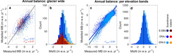
The modelled surface mass balance of the Scandinavian and Icelandic glaciers is generally in good agreement with observations (Fig. 4 and Table 2), and the performance metrics are in line with the results of other regional-scale studies (e.g. Zekollari and others, Reference Zekollari, Huss and Farinotti2019; Rounce and others, Reference Rounce, Hock and Shean2020a). Considering glacier-wide surface observations, the RMSE is 0.68 m w.e. a−1 for Scandinavia and 0.72 m w.e. a−1 for Iceland. The bias for the two regions, is +0.19 and –0.04 m w.e. a−1, respectively, whilst the corresponding r 2 are of 0.61 and 0.47. MASD = 0.56 for Scandinavia and MASD = 0.67 for Iceland, which we interpret as a reasonable, albeit far from perfect, model performance.
Evaluation of modelled mass balance versus direct observations. Colours tending to red represent Icelandic glaciers, colours tending to blue represents Scandinavian glaciers. Panels a and b show the annual glacier-wide mass balance. Panels c and d show the annual mass-balance per elevation band. The continuous line in panel c displays a linear regression of the data. In all panels, the dotted line shows the zero misfit. r $^2_{\rm Scan}$ and r $^2_{\rm Icel}$
 are the correlation coefficients for Scandinavia and Iceland, respectively. ‘MB’ stands for the mass balance.

For elevation band observations, the RMSE for Scandinavia is 1.08 m w.e. a−1 (no such data is available for Iceland), with a bias of 0.15 m w.e. a−1 and r 2 = 0.81. In this case, we find MASD = 1.1, which is rather large. A comparison between observed and modelled surface mass balance (Fig. 4c) indicates that the surface mass-balance gradient (i.e. the rate of change of mass balance with elevation) is slightly overestimated when using ERA-I and ERA-5, whilst it is closely matched when using E-OBS. Indeed, the slopes of the linear relations are of 0.85, 0.86 and 1.01, respectively. Glacier-wide surface winter balance (Fig. S3) is underestimated for Scandinavia, with an average bias of 0.53 m w.e. a−1, equivalent to ~27% of the observed winter balance (1.94 m w.e. a−1 on average). This bias is principally caused by a strong mismatch using E-OBS (bias of 0.80 m w.e. a−1). We attribute this underestimation to (1) a difference between the timing at which the modelled accumulation is evaluated and the timing of the in-situ measurements, and (2) the lower precipitation in the E-OBS data set compared to the ERA re-analyses, which increases the bias (Fig. 2 and Table 2). For Iceland, instead, the modelled winter balance is in good agreement with observations (1.61 m w.e. a−1 on average), with a bias of only –0.09 m w.e. a−1.
Length change
As for surface mass balance, the model's ability to reproduce glacier length changes is assessed against observations provided by the WGMS (WGMS, Reference WGMS2019). We use length-change observations for the period 1996–2016 (period where all glacier were transiently modelled). For each glacier with observations, comparisons are performed over time frames ranging between 10 and 15 years (Fig. 5). The time-frame length is chosen such that both modelled and observed geometry changes are statistically relevant and is meant to increase the number of comparisons (since not every glacier has an observation every year).
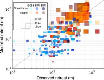
Modelled vs observed length changes between 1996 and 2016. The period covered for the individual glaciers is between 10 and 15 years. The size of the boxes represent the glacier length at inventory date.

The observed overall trend in negative length changes is well reproduced, albeit with a large spread in the values for individual glaciers (Fig. 5). The average RMSE is 127 m for Scandinavia and 281 m for Iceland, with an average bias of –59 and +97 m, respectively (equivalent to 37 and 30% of the average length change observed in the two regions). These biases in length changes indicate a slight underestimation of glacier retreat for Scandinavia and a tendency to somewhat overestimate the retreat for Iceland. The corresponding r 2 values are 0.30 and 0.45. The MASD is 1.02 for Scandinavia and 0.55 for Iceland, indicating better model performance for the latter region. Some particularly large outliers occur both in term of length change overestimation and underestimation. For some larger glaciers, in Iceland, the chosen horizontal model resolution, defined as 1/100th of the glacier length, is relatively coarse (i.e. between 200 and 500 m), and might in part explain the mismatch between observed and modelled length changes (dashed grey rectangle in Fig. 5).
Ice flow velocities
Modelled velocities are evaluated against velocity data retrieved from remote sensing. For Scandinavia, such data have been extracted from optical Sentinel-2 imagery over the period 2015–18 (Nagy and Andreassen, Reference Nagy and Andreassen2019). The observational data are based on feature-tracking algorithms, and are therefore only available for snow-free surfaces. Thus, we perform our comparisons only for glacier ablation areas.
For Icelandic glaciers, measured velocities are available from NASA's MEaSUREs ITS$\_$ LIVE project (Gardner and others, Reference Gardner, Fahnestock and Scambos2019). Here, we use the 120 m resolution composite data set, which covers the 1985–2018 time period.
Modelled surface velocities are compared to velocities derived from remote sensing at the glacier-scale by considering the 99% quantile and the mean modelled velocities (Fig. 6). For Scandinavia (Iceland), comparisons are only performed for glaciers with a least 150 (5000) observation points (i.e. ‘pixels’). This is to avoid underrepresentation of observed velocities. These thresholds are arbitrary and are meant to be a compromise between the requirements dictated by glacier area, grid spacing, data coverage and quality, so that only glaciers with sufficient data are used.
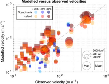
Modelled ice-flow velocities versus observations from remote sensing (Nagy and Andreassen, Reference Nagy and Andreassen2019; Gardner and others, Reference Gardner, Fahnestock and Scambos2019). Circles show the maximum glacier velocities (99% quantile), while squares represent the average glacier velocities. The symbol size is proportional to the glacier area (key given in the bottom right corner).

The results of the comparison show that, despite not being calibrated to velocity observations, our model is able to reproduce the observed surface velocities relatively well: considering the 99% quantile velocities, the RMSE is 49 m a−1 for Scandinavia and 59 m a−1 for Iceland. The bias for the two regions, is of 7 and 12 m a−1, respectively, whilst the corresponding r 2 are of 0.81 and 0.84. MASD = 0.55 for Scandinavia and MASD = 0.32 for Iceland. Note that the average of the 99% quantile observed velocity is 73 m a−1 for Scandinavia and 140 m a−1 for Iceland.
Considering the mean velocities, the RMSE is 16 m a−1 for Scandinavia and 31 m a−1 for Iceland. The bias for the two regions, is 10 and -20 m a−1, respectively, whilst the corresponding r 2 are of 0.57 and 0.72. MASD = 0.75 for Scandinavia and MASD = 0.55 for Iceland. When considering that the average of the observed velocities is 40 m a−1 for Scandinavia and 29 m a−1 for Iceland, the performance is rated as satisfactory.
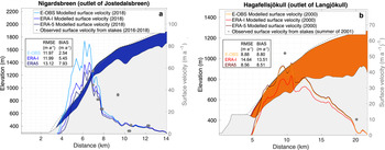
In addition to the velocity data retrieved from remote sensing, we compare the model results to in-situ velocities data obtained from repeated stake measurements. Such data exist for 14 Scandinavian glaciers (including Nigardsbreen, used here as an example) and Hagafellsjökull (eastern Iceland) (Fig. 7). For Nigardsbreen, the RMSE is 12 m a−1, with a bias of 5 m a−1. For one stake (at a distance 9.5 km from the glacier's terminus) the surface flow speed is considerably underestimated. The glacier is ~3 km wide at this location and part of the discrepancy may thus be related to the location perpendicular to the ice flow of the observation, which may not be representative for the velocity derived with our 1-D setup. Considering all 137 point velocities available for the 14 Scandinavian glaciers (mean velocity 19 m a−1) in Nagy and Andreassen (Reference Nagy and Andreassen2019), the averaged RMSE is 16 m a−1 and the bias of 11 m a−1.
Cross-section of (a) Nigardsbreen (Norway) and (b) Hagafellsjökull (Iceland) with the modelled surface geometry (2018 for Nigardsbreen, and 2000 for Hagafellsjökull). Different colours refer to the three past climate data products. Bedrock is in light grey. The grey dashed line shows the glacier geometry at the inventory year (2006 for Nigardsbreen, and 2000 for Hagafellsjökull). Observed velocities are indicated by grey dots. The observed velocities for Nigardsbreen are determined by in-situ point measurements between 2016 and 2018 (Nagy and Andreassen, Reference Nagy and Andreassen2019). For Hagafellsjökull, the measurements are from stakes observed in the summer of 2001 (Palmer and others, Reference Palmer, Shepherd, Björnsson and Pálsson2009).

For Hagafellsjökull, the RMSE between modelled and observed velocity is 11 m a−1, with a bias of 10 m a−1. This is ~30% of the mean velocity derived from the two available stake measurements (mean velocity = 31 m a−1). The discrepancy might partially be explained by the fact that the comparison is based on stake velocities measured during summer (Palmer and others, Reference Palmer, Shepherd, Björnsson and Pálsson2009). Indeed, glaciers tend to flow faster during the melting season than they do in winter (e.g. Iken and Bindschadler, Reference Iken and Bindschadler1986; Nienow and others, Reference Nienow, Sharp and Willis1998), which might explain why the modelled velocities (which refer to the annual average) are 20% slower than the measured ones.
Results
Regional future evolution
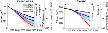
Our modelling projects show substantial ice loss for all glaciers in Scandinavia and Iceland throughout the 21st century (Figs 8, 9 and Table 3). The significant ice loss is attributed to the high summer air temperatures of the last decades and to the predicted temperature increases in the future. Compared to the 1980–2010 baseline and averaged over all past climate data products, temperatures for 2070–2100 in glacierised areas are projected to increase by 1.1 ± 0.2°C in RCP2.6, 1.9 ± 0.1°C in RCP4.5 and 3.5 ± 0.1°C RCP8.5 (Fig. 2). Scandinavian glaciers are projected to lose between 31 ± 13% (RCP2.6) and 41 ± 13% (RCP8.5) of their 2018 ice volume (272 ± 52 km3) by 2050, and between 67 ± 18% (RCP2.6) and 90 ± 7% (RCP8.5) by 2100. For Icelandic glaciers, the results anticipate losses between 16 ± 5% (RCP2.6) and 21 ± 5% (RCP8.5) by 2050, and between 43 ± 11% (RCP2.6) and 85 ± 7% (RCP8.5) by 2100 (the ice volume estimated for 2018 is of 3629 ± 605 km3). In this case, the results refer to future simulations driven by RCMs whilst the uncertainty range corresponds to one standard deviation.
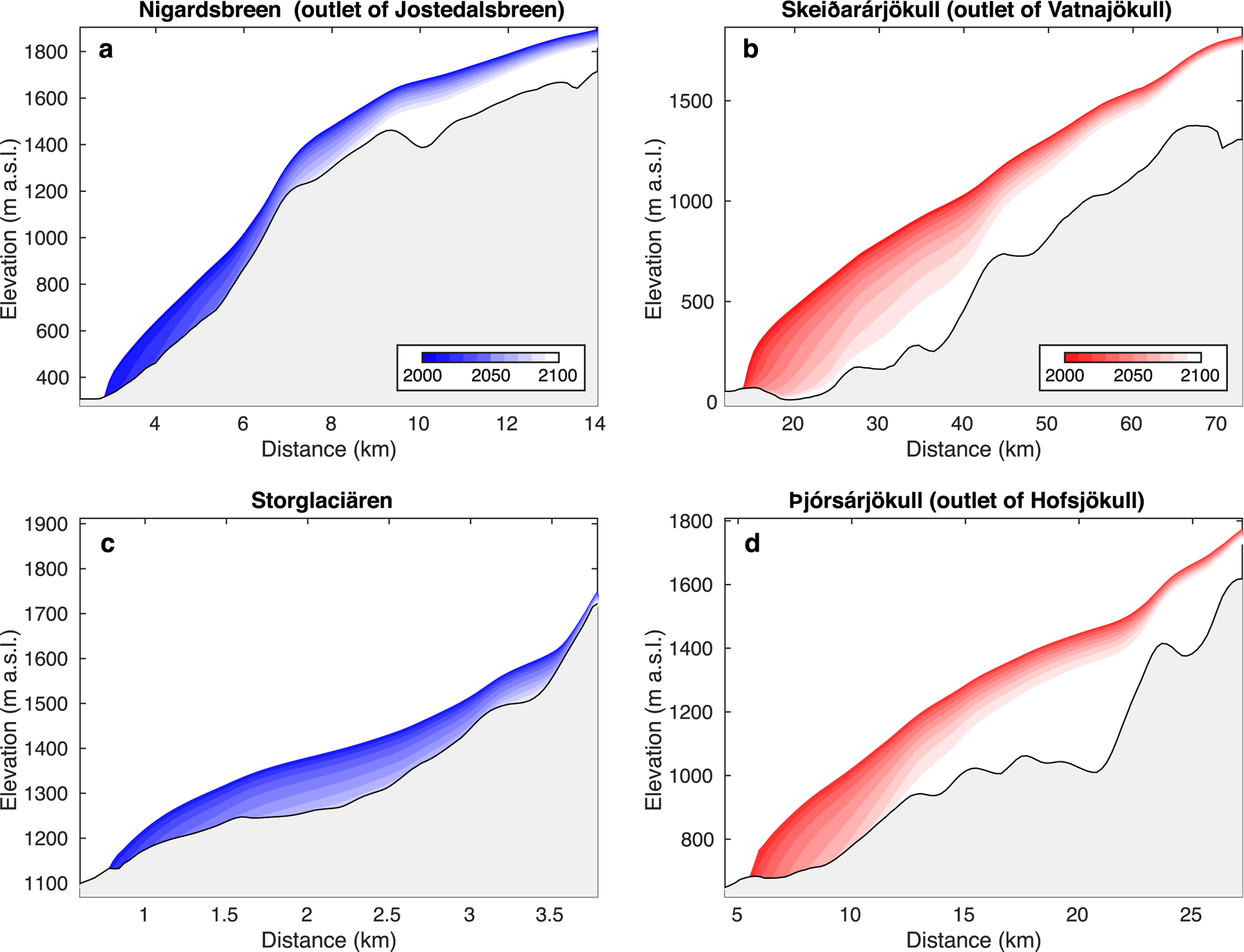
Future evolution of (a) Nigardsbreen (Scandinavia), (b) Skeiđarárjökull (Iceland), (c) Storglaciären (Scandinavia) and (d) Þjórsárjökull (Iceland). The 2000–2100 evolution is shown as the average of all RCP4.5 model members using E-OBS for the past and RCMs for the future.
Modelled volume evolution of all glaciers in (a) Scandinavia and (c) Iceland. For every RCP, the thick line represents the mean using all past climate data products and RCM as future climate projection. The transparent bands correspond to the standard deviation of all climate model members. The modelled ice volume fraction that remains in the subregions by 2100 is shown in panels b and d. The percentages are relative to the volume in 2018. The black continuous lines in (a and c), and the black squares in (b and d), represent the committed loss under 1998–2018 climatic conditions. Note that there is one such line and square for each past climate data products.

Overview of model results for Scandinavian and Icelandic glaciers

A different combination of climate forcing products is provided separately. The results show the relative ice volume change compared to 2018. The numbers refer to the average and the standard deviation of all climate model members. The AVG in the last set of rows shows the average of all past climate data products.
We also compute committed ice losses (Marzeion and others, Reference Marzeion, Kaser, Maussion and Champollion2018) for both regions by continuously forcing our model with the climate conditions occurring between 1998 and 2018. When doing so, we obtain a glacier volume loss by the end of the century of 45 ± 1% for Scandinavia and 20 ± 2% for Iceland. The differences in the temporal evolution of Scandinavian and Icelandic glaciers result from the differences in glacier volume, area and hypsometry (Fig. 1). Even if Scandinavian glaciers are more numerous compared to Icelandic ones (3413 versus 568), and even if this difference becomes larger if considering that the RGI divides ice caps into individual glaciers, the total volume of the former is about 13 times smaller than the latter, while the area is about 4 times smaller (Farinotti and others, Reference Farinotti2019a; RGI Consortium, Reference RGI Consortium2017). This implies a strong difference in mean ice thickness, which in turn results in different response times (Figs S4, S5), see Zekollari and others (Reference Zekollari, Huss and Farinotti2020) for more details.
Glacier evolution in selected subregions
To further investigate spatial differences in glacier response, Scandinavia and Iceland are subdivided into subregions (Fig. 1). For Scandinavia, we rely on the three GTN-G second-order regions (GTN-G, Reference GTN-G2017). Subregion 1 in the north and subregion 2 in the south-west have a generally higher winter precipitation compared to subregion 3 in the south-east (Fig. S6). The former two subregions are influenced by a more maritime climate, the variations of which are mainly controlled by the strength of the westerlies and by the North Atlantic Oscillation (NAO) (Laumann and Nesje, Reference Laumann and Nesje2014). Instead, the winter precipitation in subregion 3 is strongly connected to low pressure systems, which bring moist air to the eastern side of the Scandinavian mountains (Nesje and others, Reference Nesje, Bakke, Dahl, Lie and Matthews2008).
For Iceland, the RGI does not provide any subdivision, and we therefore divide the region based on the main climatic pattern. In winter, precipitation prevailingly arrives with southerly winds (Björnsson and Pálsson, Reference Björnsson and Pálsson2008). As a consequence, SW Iceland has a higher average winter precipitation compared to the NE (Fig. S7). We chose to subdivide Iceland into two subregions: subregion 2 covers the NE (>65N, >21W, while subregion 1 covers the rest of Iceland (<65N, <21W, see Fig 1).
For Scandinavia, a clearly distinct glacier evolution occurs for the three subregions: compared to 2018 and under RCP2.6, the ice volume fraction lost by 2100 in subregions 1, 2 and 3 is expected to be 63 ± 19%, 56 ± 20% and 86 ± 13%, respectively (Fig. 9). The differences between the regions are less pronounced under RCP8.5, as here all regions become largely ice-free by the end of the century. Beyond the different glacier hypsometries (Figs 1, S4 and S5), the difference in the future glacier evolution for the subregions can in part also be attributed to the precipitation patterns during the last decades. Indeed, winter precipitation in Scandinavia's west (subregions 1 and 2) was more above normal than it was in the inland regions (subregion 3) (Laumann and Nesje, Reference Laumann and Nesje2014). The above-average precipitation started in the 1960s has been attributed to strong westerlies and a positive phase of the NAO index (Laumann and Nesje, Reference Laumann and Nesje2014). This effect is clearly visible in the E-OBS data set (Fig. S6), where the average precipitation over glacierised areas in subregion 2 increased by ~0.1 m month−1 between 1950–70 and 1990–2010. On the contrary, both subregions 1 and 3 showed a lower increase of around 0.06 m month−1.
Also for Iceland, a contrasting behaviour is modelled for the two subregions. Here, the difference in future evolution is mainly driven by the different glacier characteristics (subregion 1 comprises all major Icelandic ice caps, while subregion 2 mainly features small valley glaciers), which influences glaciers responses (Belart and others, Reference Belart2020), and by the climatic conditions which show higher precipitation for subregion 1 than for subregion 2 (Fig. S7). The different glacier characteristics are most prominent when comparing the average glacier size: despite the similar number of glaciers in subregions 1 and 2 (333 versus 235), the area (10,875 and 148 km2) and volume (3580 and 6 km3) at the inventory year are strongly contrasting. Similar is true for the elevation ranges and the mean ice thickness, with the latter diverging by a factor of about ten between the two regions (Figs 1, S4 and S5). These diverging characteristics also influence the glaciers’ response time to climate variations (Belart and others, Reference Belart2020), and are reflected in the projected future evolution. For subregion 1, ice volume losses of 41 ± 11% (RCP2.6), 60 ± 12% (RCP4.5) and 85 ± 7% (RCP8.5) are modelled between 2018 and the end of the century. For subregion 2, instead, the losses are of 79 ± 19% (RCP2.6), 89 ± 9% (RCP4.5) and 95 ± 3% (RCP8.5), i.e. significantly higher than for subregion 1.
It is also important to note that the strong presence of ice caps in subregion 1 might pose a challenge for the 1-D-setup of our ice-flow model. In particular, the interplay between an ice cap's neighbouring outlet glacier cannot be captured. Comparison to more specific studies based on full 3-D modelling (see Discussion Section) shows that for ice caps our projections for future volume loss are at the upper end of the spectrum.
Impact of climate forcing products on future glacier evolution
The climate described by the past climate data products varies significantly. This is particularly true for winter precipitation (Fig. 2). For Scandinavian glaciers, for instance, the E-OBS 1979–2018 average winter precipitation (1 October–30 April) is 23% lower compared to ERA-I and ERA-5 (the two ERA data sets have roughly the same values). For Icelandic glaciers, instead, the ERA-5 winter precipitation shows 45% higher precipitation than for E-OBS and ERA-I (showing roughly the same values, Fig. 2d). Summer temperatures (1 May – 30 September) on both Scandinavian and Icelandic glaciers are more consistent, with a standard deviation of the temperature between the three data sets of 0.39 °C for the period 1979–2018. It is important to note that, due to our calibration procedure, these contrasting precipitation and temperature patterns do not directly affect the computed glacier mass balances. Indeed, fitting of the model parameters to the glacier-specific observations allows for the climate conditions extracted from the relatively coarse-scale past climate data products to be adjusted to the mass changes measured in situ. Yet, the past climate data products affect the evolution of glaciers through (1) its climatic forcing before 2018, which influences the past glacier evolution, and (2) the de-biasing procedure, which adjusts the future climate projections (see Data section).
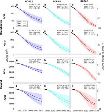
Fig. 10 shows how Scandinavian and Icelandic glaciers are modelled to evolve in the future when different climate forcing products are used as forcing. For both regions and all RCPs, model runs calibrated using E-OBS shows stronger ice volume loss by the end of the 21st century than model runs calibrated with ERA-I or ERA-5, which shows similar volume losses. On average for Scandinavia and Iceland, the differences are of 9.2, 7.7 and 4.5% for RCP2.6, RCP4.5 and RCP8.5, respectively. These differences can be attributed to differing temperature and precipitation changes between the calibration period 2003–14 and the future (Fig. S8).
Modelled evolution of the ice volume for all glaciers in (a–f) Scandinavia and (g–l) Iceland. Each line is a simulation produced by using a different past climate data set (E-OBS, ERA-I and ERA-5). Panels a–c and g–i use RCMs outputs as future climate projection, panels d–f and j–l use GCMs. The transparent bands correspond to the standard deviation of all climate model members used in one the simulations.
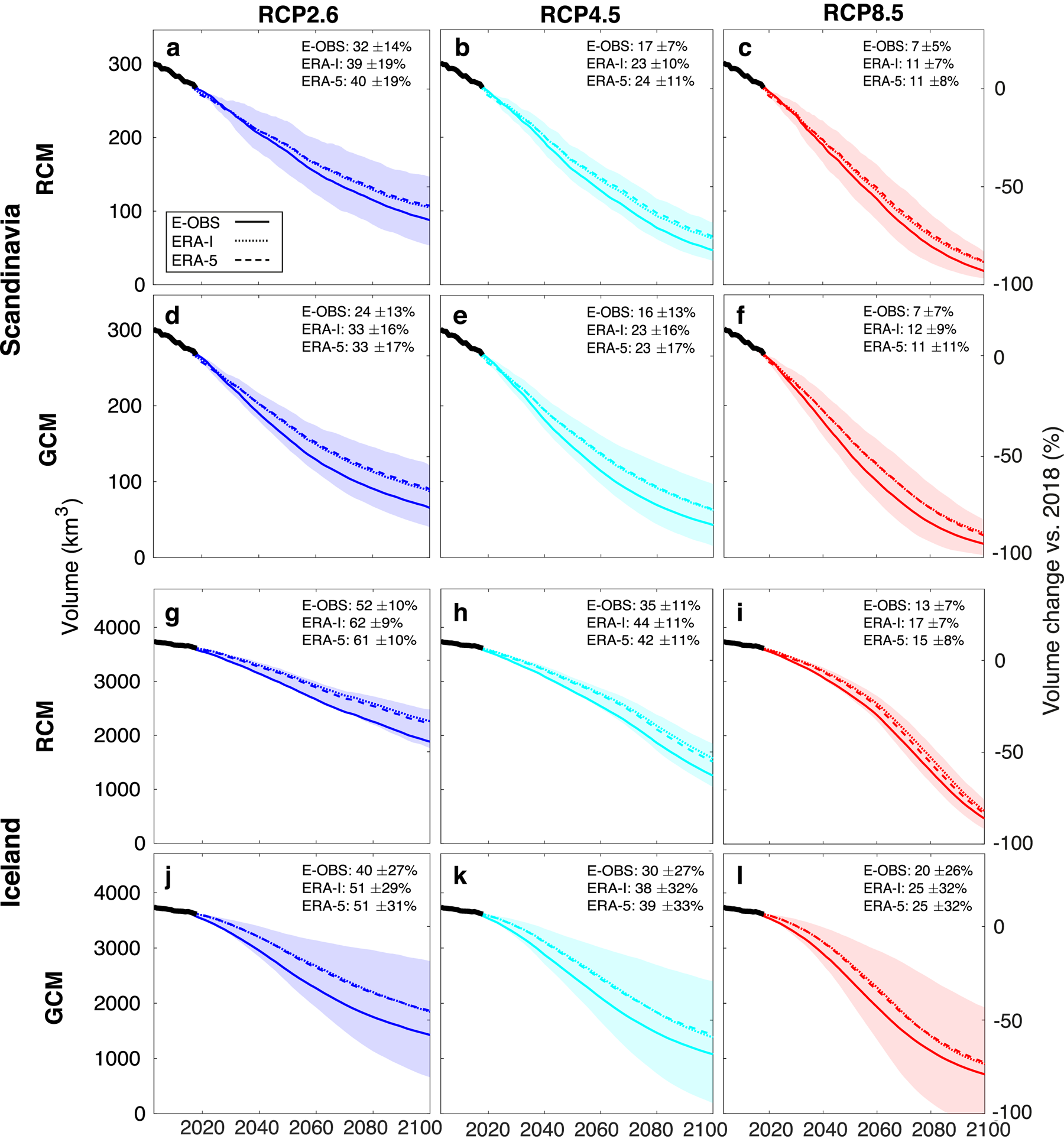
Whilst the past climate data products affect model calibration, the future climate projections directly influence the modelled glacier evolution by determining the future forcing (Fig. 10). GCMs generally show a higher ice volume loss by 2100 compared to RCMs, with differences of 8.7, 2.6 and –4.5% for RCP2.6, RCP4.5 and RCP8.5, respectively (numbers refer to the average over Scandinavia and Iceland). The differences can be attributed to diverging temperature and precipitation projections. Indeed, even if GCMs produce a stronger winter precipitation increase compared to RCMs, they also show a higher summer temperature increase resulting in more negative glacier balances (Fig. S8).
It must be noted, however, that the spread caused by the combination of different climate forcing products is small when compared to the spread between individual model members of the same climate data set (see Fig. 10). Indeed, the standard deviation of the results given by different climate model members is about three times larger than the standard deviation of the results obtained with different climate forcing products.
Discussion
Comparison with other studies
We compare our results to the outcomes of the Glacier Model Intercomparison Project (GlacierMIP, Marzeion and others, Reference Marzeion2020), which include projections of annual glacier mass change for Scandinavia and Iceland from seven different global glacier models (van de Wal and Wild, Reference van de Wal and Wild2001; Marzeion and others, Reference Marzeion, Jarosch and Hofer2012; Radić and Hock, Reference Radić and Hock2014; Huss and Hock, Reference Huss and Hock2015; Sakai and Fujita, Reference Sakai and Fujita2017; Maussion and others, Reference Maussion2019; Shannon and others, Reference Shannon2019). These models had different spatial resolutions, and used different methods for calculating the glacier mass balance, for de-biasing the climatic input data (see Data section), or for computing glacier geometry changes.
Our results are generally in the mid-range of the GlacierMIP projections for Scandinavia, while we project a higher mass loss for Iceland (Fig. 11). The higher loss for Iceland can in part be attributed to the fact that most of the region's ice volume is located in ice caps (Björnsson and Pálsson, Reference Björnsson and Pálsson2008), which show a different evolution when compared to mountain glaciers. Indeed, volume-area scaling approaches – used by most of the models included in GlacierMIP (Marzeion and others, Reference Marzeion2020) – are designed for glaciers, and generally fail to reproduce ice cap changes. Similarly, the mass conserving retreat parameterisation used by Huss and Hock (Reference Huss and Hock2015) and Rounce and others (Reference Rounce, Hock and Shean2020a) for example, assumes that elevation change in the glaciers’ highest parts is minor. This leads to near-constant elevations of ice cap summits even with a warming climate, which in turn causes the mass-balance-elevation feedback (Edwards and others, Reference Edwards2014; Åkesson and others, Reference Åkesson, Nisancioglu, Giesen and Morlighem2017) to be underestimated. In our approach, glaciers and ice cap geometries are evolving through time, as prescribed by the local ice flow, mass balance and mass conservation. This causes the elevation of ice cap summits to decrease through time as climate warms, resulting in a positive feedback between surface elevation and mass balance, as a lowering of the surface elevation leads to higher temperatures and thus more melt (see Fig. S9). That said, we acknowledge that our SIA approach has limitations for fast-flowing glaciers (Zekollari and others, Reference Zekollari, Huybrechts, Noël, van de Berg and van den Broeke2017), which might influence the modelling of outlet glaciers from ice caps. Similarly, the geometrical simplifications that are necessary for 1-D modelling approaches might introduce some biases in the projected evolution. In this respect, a comparison with the 3-D modelling work by Schmidt and others (Reference Schmidt2020) suggests that these biases tend towards larger ice loss (see below).
Comparison of modelled volume changes with values from Marzeion and others (Reference Marzeion2020). Changes are expressed with respect to the 2015 baseline, i.e. 276 ± 52 km3 for Scandinavia (a) and 3658 ± 611 km3 for Iceland (b). From left to right, the abbreviations (GLIMB, GloGEM, JULES, MAR2012, OGGM, RAD2014, WAL2001) stand for van de Wal and Wild (Reference van de Wal and Wild2001); Marzeion and others (Reference Marzeion, Jarosch and Hofer2012); Radić and Hock (Reference Radić and Hock2014); Huss and Hock (Reference Huss and Hock2015); Sakai and Fujita (Reference Sakai and Fujita2017); Maussion and others (Reference Maussion2019); Shannon and others (Reference Shannon2019), respectively. Note that the results of this study (far right of each panel) are subdivided for simulations driven by RCM and GCM model output.

A direct comparison between our simulations and modelling studies performed for individual glaciers (e.g. Oerlemans, Reference Oerlemans1997; Marshall, Reference Marshall2005; Aðalgeirsdóttir and others, Reference Aðalgeirsdóttir, Jóhannesson, Björnsson, Pálsson and Sigurðsson2006; Laumann and Nesje, Reference Laumann and Nesje2009a, Reference Laumann and Nesje2009b; Andreassen and Oerlemans, Reference Andreassen and Oerlemans2009; Giesen and Oerlemans, Reference Giesen and Oerlemans2010; Laumann and Nesje, Reference Laumann and Nesje2014; Schmidt and others, Reference Schmidt2020) is not straightforward since different climate scenarios and boundary conditions are used. Still, Table 4 provides a compilation of such individual studies and shows that, in general, our results are in the range of previous findings.
List of glacier-specific modelling studies performed for Scandinavia and Iceland, and comparison with results obtained in this study

The column ‘Previous study’ shows either the volume change ΔV or the length change ΔL for the time period given in the corresponding column. The column ‘This study’, shows ΔV or ΔL in the same time period as the glacier-specific study (or for the period 2000–2100 if ‘Time’ is labelled with an asterisk *) for RCP2.6, 4.5 and 8.5. The column ‘Comp.' shows a comparison between the two results. The symbols ‘=’, ‘–’ and ‘+’ indicate a difference within ± 10 %, < –10 % and > 10 %, respectively.
In light of the significance of ice caps in Iceland's subregion 1, a more detailed comparison was performed for six outlet glaciers of Vatnajökull (the largest ice cap of Iceland) against the study by Schmidt and others (Reference Schmidt2020). Schmidt and others (Reference Schmidt2020), forced the 3-D glacier ice-flow model PISM (a model based on the SIA and shallow shelf approximations, Reference Bueler and Brown2009) with surface mass-balance time series obtained from the HARMONIE–AROME reanalysis for the past and both the EC-Earth forced HIRHAM5 GCM and the CORDEX ensemble for the future. The results of the two studies differ considerably, with our results showing significantly faster and more pronounced mass loss than Schmidt's (Fig. S10). We attribute the difference to a combination of reasons: For one, the two studies used different bedrock topographies; Schmidt and others (Reference Schmidt2020) used a topography including local radio-echo soundings whilst our topography is based on modelling constrained by regional ice thickness data, ice flow, and, therefore mass turnover. For another, Schmidt and others (Reference Schmidt2020) provide results along a central flowline whilst our simulation happens along elevation bands. This makes a direct comparison difficult. It should also be noted that whilst our 1-D flowline approach neglects the effects of lateral dynamics captured by the 3-D simulations of Schmidt and others (Reference Schmidt2020), the latter does not explicitly account for a process that is accounted for in our results: the mass-balance feedback. This process, indeed, is important when surface elevation changes are large, as a strong lowering of the glacier surface causes the surface to reside at elevations with higher temperatures, which in turn affects surface mass balance through both enhanced ablation and reduced accumulation. The latter is particularly important for the relatively flat accumulation areas typical for ice caps, and our results indicate that the effect can be significant for the evolution of Dyngjujökull and Tungnaárjökull, for example (Fig. S10). Whilst there is the possibility that the simplifications caused by our 1-D model setup might overestimate the effect (in general, our results agree better with other 1-D based studies than they do with 3-D models; see Table IV), the combination with the different bedrock topographies seem to explain the smaller volume loss and glacier retreat as projected by Schmidt and others (Reference Schmidt2020) when compared to our study.
Sensitivity analysis
Uncertainties in glacier projections can arise from a number of factors. Here, we quantify the sensitivity of our results to variations in (i) initial ice-thickness distribution, (ii) the method of geometry initialisation, (iii) mass-balance calibration data and (iv) model parameters. The sensitivity experiments all refer to results driven by an E-OBS for the past and one selected RCM member for the future. In particular, we use the RCM ‘CCLM4-8-17’ and its realisation ‘r1i1p1’ for RCP4.5, driven at its boundary by the GCM ‘CNRM-CM5-LR’. We chose this particular realisation since it has been identified as to represent a median climate evolution (Jacob and others, Reference Jacob2014; Kotlarski and others, Reference Kotlarski2014).
Ice-thickness distribution
The future evolution of glaciers strongly depends on the initial ice thickness used for modelling (Gabbi and others, Reference Gabbi, Farinotti, Bauder and Maurer2012; Farinotti and others, Reference Farinotti2019a). To test model sensitivity to the initial ice-thickness distribution, we project the future evolution of Scandinavian and Icelandic glaciers by assuming two cases: one where the ice is thicker and one where the ice is thinner as compared to the simulations presented so far. To obtain these adjusted distributions, we add (and subtract) the standard deviation of the multi-model ensemble provided by Farinotti and others (Reference Farinotti2019a) (i.e. 19% for Scandinavia and 23% for Iceland). The discrepancies between individual ensemble members are predominantly due to the sparse observations that are publicly available for the two regions. Indeed, ice-thikness observations are so far retrievable only for ca. 28% of the Scandinavian and 20% of the Icelandic glacier areas (Björnsson and Pálsson, Reference Björnsson and Pálsson2008; Andreassen and others, Reference Andreassen, Huss, Melvold, Elvehøy and Winsvold2015; Welty and others, Reference Welty2020).
The sensitivity tests indicate that the relative volume loss between 2018 and 2100 is affected only little by the initial ice thickness: For Scandinavia, 68 and 74% of the volume is lost for the thinner and thicker ice, respectively, which is similar to the reference loss of 71%. For Iceland, the corresponding numbers change to 47 and 57%, which is again similar to the reference loss of 51%. These results thus indicate that the effect of the ice thickness uncertainty is in the range of that of the climate forcing products.
Initialisation method and initial steady-state assumption
Zekollari and others (Reference Zekollari, Huss and Farinotti2019) showed that using a different calibration and initialisation procedure has a minor effect on the 21st century ice loss modelled for glaciers in the European Alps. Here, we further analyse this by comparing the results from our initialisation strategy (see Methods section) to the initialisation method of Zekollari and others (Reference Zekollari, Huss and Farinotti2019). In the work by Zekollari and others (Reference Zekollari, Huss and Farinotti2019), the 1961–90 climatic conditions are used to create an initial, fictive steady state for the year 1990. In our approach, instead, the date of the initial steady state is glacier-specific, and dependent on both the glacier response time and the climate (see Supplementary Chapter S1).
The comparison of the results generated by using the two different approaches shows that the sensitivity to the initialisation procedure is low. Indeed, the differences in modelled 2018–2100 ice loss are of only ca. 2% for Scandinavia, and of <1% for Iceland. This confirms the robustness of both methods, and indicates that the timing of the steady-state period does barely influence the future glacier evolution as long as it is set sufficiently far (typically half the glacier's response time in our approach or before 1990 in Zekollari and others, 2019) back in the past.
Surface mass-balance calibration
The model was calibrated with glacier-specific geodetic ice volume changes that are subject to typical uncertainties of 0.26 m w.e. a−1 (Scandinavia) and 0.32 m w.e. a−1 (Iceland) (Zemp and others, Reference Zemp2019). To investigate the effect of this uncertainty, we randomly varied the geodetic mass balance assigned to every glacier within the stated uncertainties.
This sensitivity test yields a discrepancy in the modelled 2018–2100 relative volume loss of 3% for Scandinavia, and of <1% for Iceland. This indicates that even though the glacier-specific results directly depend on the glacier-specific calibration data, random variations witin the observational uncertainty do not systematically influence the regional estimates. We acknowledge that this analysis only considers independent, random uncertainties, whilst spatially correlated uncertainties might exist.
In addition to the above, we performed a dedicated analysis targeting at the sensitivity of our results to the scheme used for assigning geodetic mass balances to unmeasured glaciers. To do so, we use a cross-validation scheme in which we remove the geodetic observations for one-third of all glaciers, and use the interpolation scheme presented in the Data section to assign a mass-balance estimate to them. This procedure is repeated three times, thus yielding an error estimate for every glacier. The analysis shows that the difference in the relative volume loss modelled for 2018–2100 is <1% for Scandinavia, and <3% for Iceland. This indicates that the overall results are only marginally affected by the necessity of interpolating observations to some unmeasured glaciers.
Model parameters
Following Huss and Hock (Reference Huss and Hock2015), the ratio between DDF snow and DDF ice was set to 2 in this study. To analyse how this ratio affects the computed mass balances, we re-run the model by using a ratio of 2.5. The results indicate that varying this empirical factor does not significantly impact the modelled 21st century volume loss: changes in projected regional volume loss are <1% in both Scandinavia and Iceland.
In the mass-balance calibration procedure, the precipitation enhancement factor was varied from 0.8 to 2.0 for Scandinavia, and from 1.8 to 3.0 for Iceland. We analyse the effect of changing this range to 1.4–2.6. When doing so and compared to the standard run, differences in modelled 2018–2100 ice loss decrease by 1% for Scandinavia and increase by 4% for Iceland. This shows that also variations in the precipitation enhancement factor do not substantially influence the future evolution of glaciers in these regions. That said, it must be noted that such changes in precipitation can have a more substantial effect on mass turnover (since an enhancement in modelled precipitation can be compensated by enhanced ablation). This can in turn impact the modelled ice-flow dynamics and the coresponding ice-flow velocities (see Fig. 6).
Conclusions
In this paper, we modelled the future evolution of all Scandinavian and Icelandic glaciers using a coupled mass-balance ice-flow model. A new model initialisation procedure was designed, which is glacier specific and accounts for both glacier response time and climate. To analyse the model's sensitivity to climate input and to assess future mass loss, the model was forced with three different past climate data products (E-OBS, ERA-I and ERA-5) and with future climate projections obtained from both GCMs and RCMs. Modelled mass balance was calibrated using glacier-specific geodetic mass changes derived from remote sensing, and was evaluated with independent in-situ mass-balance measurements. As a part of the evaluation procedure, we also compared modelled and observed ice-flow velocities and glacier length changes.
Our model results indicated that, compared to 2018, Scandinavian glaciers are expected to lose between 67 ± 18% (RCP2.6) and 90 ± 7% (RCP8.5) of their ice volume by 2100. In the same period, Icelandic glaciers are expected to lose between 43 ± 11% (RCP2.6) and 85 ± 7% (RCP8.5). In both regions, the spread of the results provided by different RCPs is large, and important differences in the future glacier evolution are found between subregions. This is due to differences in both climate conditions and glacier hypsometries. By using different climate forcing, in order to analyse model sensitivity to different climate data sets, our results indicate that the variations induced by different forcing products are a factor of three smaller than the spread between different model members within a given RCP scenario. We attribute this to our model calibration strategy that relies on observed glacier-specific mass balances, as it offsets possible biases in the climate data. This result implies that considering different climate forcing product is only of minor importance when generating projections of future glacier evolution, as opposed to accurate data to calibrate the model at the glacier-specific scale. We cannot exclude, however, that for other regions with a potentially higher discrepancy between climate forcing products, the choice of the data set may have a larger effect.
Apart from Iceland's ice cap dominated south, where our simplified 1-D model projects substantially higher volume losses than more detailed 3-D studies (e.g. Schmidt and others, Reference Schmidt2020), our simulations agree well with earlier, glacier-specific studies. Consequently, our regional estimates are in line with previous results for Scandinavia but show higher mass losses for Iceland. We mainly attribute this to the representation of ice caps. Whilst our results might neglect some of the effects caused by ice dynamics – such as the possible migration of ice divides – our model takes into account the surface-elevation feedback on mass balance. This is different than what was done in previous studies relying on volume–area scaling relations or retreat parameterisations, and shows the importance of taking ice dynamics into account when modelling large glaciers and ice caps. We suggest that such explicit accounting for ice dynamics will be crucial to improve the estimates of glacier contribution to the 21st century sea-level change.
Supplementary material
The supplementary material for this article can be found at https://doi.org/10.1017/jog.2021.24.
Acknowledgments
We are grateful to the Swiss National Science Foundation, and for the funding provided for project no. 184634 in particular. HZ acknowledges the funding from a Marie Skłodowska-Curie Individual Fellowship (grant 799904). We thank the RGI consortium for the global glacier inventory data. We acknowledge the ECA&D project for the E-OBS data set, ECMWF for the ERA-I and ERA-5 re-analysis, and CMIP for the GCM and RCM outputs. We also thank the WGMS for providing mass balance and length change measurements, T. Nagy and L.M. Andreassen for providing glacier velocity maps for Scandinavia, and the ITS$\_$ LIVE project for providing the same for Iceland. Finally, we are very thankful to the three anonymous reviewers, and the scientific editor, Marius Schaefer, whose detailed comments and suggestions have greatly helped to improve this manuscript.
Author contributions
LC performed the numerical modelling with support from HZ, MH and DF. The original code was developed by HZ (ice flow component) and MH (mass balance component). LC, HZ, MH and DF conceived the study. LC developed the new initialisation procedure with input from HZ, MH and DF. LC wrote the manuscript and produced the figures, with contributions from all co-authors.


 Open access