


1. Introduction
Earth system models have considerable potential to incorporate extensive biogeochemistry–climate interactions between the atmosphere and ocean ecosystems to aid marine management (Bonan & Doney, Reference Bonan and Doney2018). The atmospheric sources of macronutrient nitrogen (N) and micronutrient iron (Fe) delivered to the ocean have been disturbed by human activities (Jickells et al. Reference Jickells, An, Andersen, Baker, Bergametti, Brooks, Cao, Boyd, Duce, Hunter, Kawahata, Kubilay, LaRoche, Liss, Mahowald, Prospero, Ridgwell, Tegen and Torres2005; Duce et al. Reference Duce, LaRoche, Altieri, Arrigo, Baker, Capone, Cornell, Dentener, Galloway, Ganeshram, Geider, Jickells, Kuypers, Langlois, Liss, Liu, Middelburg, Moore, Nickovic, Oschlies, Pedersen, Prospero, Schlitzer, Seitzinger, Sorensen, Uematsu, Ulloa, Voss, Ward and Zamora2008). The major source of Fe from the atmosphere is mineral dust. However, pyrogenic Fe-containing aerosols have been suggested to increase the net primary production (NPP) in large parts of the open ocean because of their enhanced Fe solubilities (i.e. ratio of dissolved Fe to total Fe) during atmospheric transport (Ito et al. Reference Ito, Myriokefalitakis, Kanakidou, Mahowald, Scanza, Hamilton, Baker, Jickells, Sarin, Bikkina, Gao, Shelley, Buck, Landing, Bowie, Perron, Guieu, Meskhidze, Johnson, Feng, Kok, Nenes and Duce2019). The atmospheric Fe deposition could have a larger effect on NPP than atmospheric N in some ocean biogeochemistry models (Krishnamurthy et al. Reference Krishnamurthy, Moore, Mahowald, Luo, Doney, Lindsay and Zender2009; Okin et al. Reference Okin, Baker, Tegen, Mahowald, Dentener, Duce, Galloway, Hunter, Kanakidou, Kubilay, Prospero, Sarin, Surapipith, Uematsu and Zhu2011). However, the response of ocean biogeochemistry to changes in atmospheric Fe input depends on the relative importance of the atmospheric source to the other external sources such as continental shelf and hydrothermal sources, as well as internal sources recycled by zooplankton and microorganisms (Tagliabue et al. Reference Tagliabue, Bopp and Aumont2008, Reference Tagliabue, Aumont, Death, Dunne, Dutkiewicz, Galbraith, Misumi, Moore, Ridgwell, Sherman, Stock, Vichi, Völker and Yool2016).
Atmospheric and oceanic communities have used various definitions for different forms of Fe in aerosols and seawater (Baker & Croot, Reference Baker and Croot2010; Meskhidze et al. Reference Meskhidze, Völker, Al-Abadleh, Barbeau, Bressac, Buck, Bundy, Croot, Feng, Ito, Johansen, Landing, Mao, Myriokefalitakis, Ohnemus, Pasquier and Yein press). To avoid any confusion in tracking the effect of atmospheric Fe source on the marine Fe cycle and NPP in this study, we regard dissolved Fe (DFe) as the most readily bioavailable form of Fe, and use Fe solubility as instantaneously dissolved fraction of total Fe (TFe) input from atmospheric chemistry models to ocean biogeochemistry models. Note that this fraction includes ferrihydrite colloids, nanoparticles and aqueous species (Raiswell & Canfield, Reference Raiswell and Canfield2012).
Global atmospheric deposition fluxes of DFe into the ocean have been estimated in the range 0.14–0.43 Tg Fe a−1 (Ito et al. Reference Ito, Myriokefalitakis, Kanakidou, Mahowald, Scanza, Hamilton, Baker, Jickells, Sarin, Bikkina, Gao, Shelley, Buck, Landing, Bowie, Perron, Guieu, Meskhidze, Johnson, Feng, Kok, Nenes and Duce2019). However, global ocean biogeochemistry models use a wider range of 0.08–1.81 Tg Fe a−1, resulting from model-specific Fe content in dust and Fe solubility (Tagliabue et al. Reference Tagliabue, Aumont, Death, Dunne, Dutkiewicz, Galbraith, Misumi, Moore, Ridgwell, Sherman, Stock, Vichi, Völker and Yool2016). Fe content in aerosols depends on the mineralogical composition in clay-sized and silt-sized soils, because minerals in soils differ in their Fe content (Journet et al. Reference Journet, Balkanski and Harrison2014). Some atmospheric chemistry models (Johnson & Meskhidze, Reference Johnson and Meskhidze2013; Myriokefalitakis et al. Reference Myriokefalitakis, Daskalakis, Mihalopoulos, Baker, Nenes and Kanakidou2015; Ito & Shi, Reference Ito and Shi2016; Scanza et al. Reference Scanza, Hamilton, Garcia-Pando, Buck, Baker and Mahowald2018) have therefore taken into account the soil mineralogy map and size distribution of Fe contents in mineral dust aerosols, and the resulting global mean Fe content in mineral dust emissions ranges from 2.6% to 3.5% (Myriokefalitakis et al. Reference Myriokefalitakis, Ito, Kanakidou, Nenes, Krol, Mahowald, Scanza, Hamilton, Johnson, Meskhidze, Kok, Guieu, Baker, Jickells, Sarin, Bikkina, Shelley, Bowie, Perron and Duce2018). Although mineral dust is the major source of DFe, the aerosol Fe solubility is extremely low at 0.4 ± 0.1% in the eastern North Atlantic near the Saharan dust source regions (Ito et al. Reference Ito, Myriokefalitakis, Kanakidou, Mahowald, Scanza, Hamilton, Baker, Jickells, Sarin, Bikkina, Gao, Shelley, Buck, Landing, Bowie, Perron, Guieu, Meskhidze, Johnson, Feng, Kok, Nenes and Duce2019). Further away from the source regions, much higher Fe solubility is derived from the multiple field campaigns (up to 98%). While no consensus has emerged on the factors controlling the observed high Fe solubility for aerosols and rainwater delivered into the Southern Ocean, it has been concluded that high Fe solubility in aerosols is mainly attributed to DFe released from pyrogenic Fe oxides (Ito et al. Reference Ito, Myriokefalitakis, Kanakidou, Mahowald, Scanza, Hamilton, Baker, Jickells, Sarin, Bikkina, Gao, Shelley, Buck, Landing, Bowie, Perron, Guieu, Meskhidze, Johnson, Feng, Kok, Nenes and Duce2019).
Many ocean biogeochemistry models assume a constant Fe solubility for mineral dust that is substantially higher than those measured near dust source regions, and overestimate DFe concentrations in the tropical and subtropical North Atlantic downwind of the Saharan dust source regions. Furthermore, DFe sinks such as scavenging and precipitation in the ocean models are not well constrained. The first synthesis of a global-scale dataset of DFe from 354 samples in the open ocean showed a relatively narrow range of DFe concentration, despite the wide range of atmospheric inputs (Johnson et al. Reference Johnson, Gordon and Coale1997). In earlier modelling studies, therefore, no particle scavenging was assumed for DFe below 0.6 nM, presumably in the presence of strong Fe-binding ligands ubiquitously below that level (Johnson et al. Reference Johnson, Gordon and Coale1997). As more DFe measurements have become available for different locations and time periods, a wider range of DFe concentration has been observed than that accounted for by these models. Accordingly, a more detailed model including a weaker ligand and larger concentration of total ligand has led to better model–measurement agreement (Parekh et al. Reference Parekh, Follows and Boyle2004). Currently, some ocean biogeochemistry models consider variability in Fe-binding ligands (Misumi et al. Reference Misumi, Lindsay, Moore, Doney, Tsumune and Yoshida2013; Völker & Tagliabue, Reference Völker and Tagliabue2015; Pham & Ito, Reference Pham and Ito2018), although some still assume a constant ligand concentration of 0.6 or 1 nM (Tagliabue et al. Reference Tagliabue, Aumont, Death, Dunne, Dutkiewicz, Galbraith, Misumi, Moore, Ridgwell, Sherman, Stock, Vichi, Völker and Yool2016). Furthermore, few ocean biogeochemistry models consider scavenging of Fe onto mineral dust, in addition to the scavenging on organic particles (Moore & Braucher, Reference Moore and Braucher2008; Aumont et al. Reference Aumont, Ethé, Tagliabue, Bopp and Gehlen2015; Ye & Völker, Reference Ye and Völker2017; Pham & Ito, Reference Pham and Ito2018). Consequently, there are large uncertainties in the effects of atmospheric input of DFe on seawater DFe (Tagliabue et al. Reference Tagliabue, Aumont, Death, Dunne, Dutkiewicz, Galbraith, Misumi, Moore, Ridgwell, Sherman, Stock, Vichi, Völker and Yool2016).
Here, we use one atmospheric chemistry transport model and two ocean biogeochemistry models to investigate the effects of atmospheric deposition of DFe from mineral dust and combustion aerosols on ocean biogeochemistry. The choice of two different ocean biogeochemistry models is intended to demonstrate the uncertainties associated with the assumptions of sources and sinks of DFe in ocean models. The models are referred to in this study as Model H and Model L after their high and low sensitivities to atmospheric inputs of DFe, respectively. Section 2 provides background information on mineral dust and combustion aerosols as sources of DFe to the surface ocean. Section 3 describes the modelling approaches and numerical experiments performed in this study. The results of different simulations are provided in Section 4 to explore the effects of different DFe sources (i.e. lithogenic v. pyrogenic sources and atmospheric v. sedimentary inputs) on DFe in the surface ocean and marine productivity. Section 5 presents a summary of our findings and discusses the future outlook.
2. Lithogenic and pyrogenic Fe-containing aerosols
Different emission and atmospheric transformation processes affect Fe solubilities in ambient aerosols (Fig. 1). The aerosol Fe solubility can be affected by acidic processing during long-range transport in the atmosphere. Formation rates of DFe from Fe-containing mineral aerosols strongly depend on concentrations of proton and ligands in solutions absorbed on hygroscopic particles (i.e. aerosol waters) (Spokes et al. Reference Spokes, Jickells and Lim1994; Chen & Grassian, Reference Chen and Grassian2013; Ito & Shi, Reference Ito and Shi2016). Based on laboratory experiments for Fe-containing mineral aerosols, atmospheric chemistry transport models adopted a parameterization of DFe from mineral aerosols that involves a thermodynamic equilibrium module to estimate the acidity in aqueous phase of hygroscopic particles (Meskhidze et al. Reference Meskhidze, Chameides and Nenes2005; Ito & Feng, Reference Ito and Feng2010; Myriokefalitakis et al. Reference Myriokefalitakis, Daskalakis, Mihalopoulos, Baker, Nenes and Kanakidou2015). In the thermodynamic equilibrium calculations, the estimates of pH strongly depend on the mixing of Fe-containing aerosols with alkaline compounds such as carbonate minerals (e.g. CaCO3) and sea salt (i.e. NaCl) (Meskhidze et al. Reference Meskhidze, Chameides and Nenes2005; Ito & Xu, Reference Ito and Xu2014; Guo et al. Reference Guo, Liu, Froyd, Roberts, Veres, Hayes, Jimenez, Nenes and Weber2017). A highly acidic condition is therefore very rare for mineral dust in larger particles because alkaline minerals neutralize the acidic species in most cases (Ito & Feng, Reference Ito and Feng2010; Johnson & Meskhidze, Reference Johnson and Meskhidze2013; Myriokefalitakis et al. Reference Myriokefalitakis, Daskalakis, Mihalopoulos, Baker, Nenes and Kanakidou2015). Under higher pH conditions (>4) in oxygenated waters, Fe dissolution stops and DFe precipitates as poorly crystalline nanoparticles without strong ligands (Spokes et al. Reference Spokes, Jickells and Lim1994; Shi et al. Reference Shi, Krom, Bonneville and Benning2015). The internal mixing of alkaline components in mineral dust with Fe-containing minerals can lead to higher pH and thus suppression of Fe dissolution in atmospheric chemistry models (Ito et al. Reference Ito, Myriokefalitakis, Kanakidou, Mahowald, Scanza, Hamilton, Baker, Jickells, Sarin, Bikkina, Gao, Shelley, Buck, Landing, Bowie, Perron, Guieu, Meskhidze, Johnson, Feng, Kok, Nenes and Duce2019). As for submicron aerosols, the carbonate buffering capacity is eventually exhausted via sulphate formation from marine sources of dimethyl sulphide (DMS) during long-range transport (Ito & Xu, Reference Ito and Xu2014; Ito & Shi, Reference Ito and Shi2016).
Mechanisms and processes of Fe dissolution in aerosols.

Aerosols from combustion sources are dominated by fine-mode particles that typically have high Fe solubility and low mass concentration. Fly ash could be emitted with a large amount of acidic pollutants such as sulphate (SO4), nitrate (NO3) and oxygenated organic species. Fe in oil fly ash is mainly present as ferric sulphate salt (Fe2(SO4)3·9(H2O)) and nanoparticles, and is therefore associated with high Fe solubility observed over the oceans (Sedwick et al. Reference Sedwick, Sholkovitz and Church2007; Schroth et al. Reference Schroth, Crusius, Sholkovitz and Bostick2009; Furutani et al. Reference Furutani, Jung, Miura, Takami, Kato, Kajii and Uematsu2011; Ito, Reference Ito2013). Fe oxides emitted from coal burning are coated with sulphate during atmospheric transport and dissolved due to strong acidity in the form of Fe sulphate (Fang et al. Reference Fang, Guo, Zeng, Verma, Nenes and Weber2017; Li et al. Reference Li, Xu, Liu, Shi, Yao, Gao, Chen, Chen, Zhang, Zhang and Wang2017). In the presence of enough organic ligands, DFe is maintained in solution, resulting in relatively high Fe solubility for combustion aerosols over the ocean (Wozniak et al. Reference Wozniak, Shelley, McElhenie, Landing and Hatcher2015; Ito & Shi, Reference Ito and Shi2016).
3. Method
3.a. Atmospheric chemistry model
The three-dimensional (3D) global chemistry transport model used in this study is a coupled gas-phase (Ito et al. Reference Ito, Sillman and Penner2007) and aqueous-phase chemistry version (Lin et al. Reference Lin, Sillman, Penner and Ito2014) of the Integrated Massively Parallel Atmospheric Chemical Transport (IMPACT) model (Ito et al. Reference Ito, Lin and Penner2018). Here, we describe the methods relevant to this study. To improve the accuracy of our simulations of DFe deposition to the oceans, we have upgraded the reanalysis meteorological data (Gelaro et al. Reference Gelaro, McCarty, Suárez, Todling, Molod, Takacs, Randles, Darmenov, Bosilovich, Reichle, Wargan, Coy, Cullather, Draper, Akella, Buchard, Conaty, da Silvaa, Gu, Kim, Koster, Lucchesi, Merkova, Nielsen, Partyka, Pawson, Putman, Rienecker, Schubert, Sienkiewicz and Zhao2017) and deposition schemes (Wang & Penner, Reference Wang and Penner2009).
The model is driven by the Modern Era Retrospective analysis for Research and Applications 2 (MERRA-2) reanalysis meteorological data from of the National Aeronautics and Space Administration (NASA) Global Modeling and Assimilation Office (GMAO) (Gelaro et al. Reference Gelaro, McCarty, Suárez, Todling, Molod, Takacs, Randles, Darmenov, Bosilovich, Reichle, Wargan, Coy, Cullather, Draper, Akella, Buchard, Conaty, da Silvaa, Gu, Kim, Koster, Lucchesi, Merkova, Nielsen, Partyka, Pawson, Putman, Rienecker, Schubert, Sienkiewicz and Zhao2017) with a horizontal resolution of 2.0° × 2.5° and 59 vertical layers for the year of 2004. The IMPACT model simulates the emissions, vertical diffusion, advection, gravitational settling, convection, dry deposition, wet scavenging and photochemistry of major aerosol species, which include mineral dust, Fe-containing combustion aerosols, black carbon, organic carbon, sea spray aerosols, sulphate, nitrate, ammonium and secondary organic aerosols, and their precursor gases. We calculated dust emissions using a physically based emission scheme (Kok et al. Reference Kok, Ridley, Zhou, Miller, Zhao, Heald, Ward, Albani and Haustein2014; Ito & Kok, Reference Ito and Kok2017) while we prescribed the combustion sources (Ito et al. Reference Ito, Lin and Penner2018). A mineralogical map was used to estimate the emissions of Fe in aeolian dust (Journet et al. Reference Journet, Balkanski and Harrison2014; Ito & Shi, Reference Ito and Shi2016). Atmospheric processing of Fe-containing aerosols is predicted in four size bins (diameters: 0.1–1.26, 1.26–2.50, 2.5–5.0 and 5–20 µm) (Ito, Reference Ito2015; Ito & Shi, Reference Ito and Shi2016). The chemical composition of mineral dust and combustion aerosols can change dynamically from that in the originally emitted aerosols due to reactions with gaseous species. The aerosol acidity depends on the aerosol types, mineralogy, particle size, meteorological conditions and transport pathway of aerosols (Ito & Feng, Reference Ito and Feng2010; Ito & Xu, Reference Ito and Xu2014; Ito, Reference Ito2015; Ito & Shi, Reference Ito and Shi2016). Transformation from relatively insoluble Fe to DFe in aerosol waters due to proton-promoted, oxalate-promoted and photo-reductive Fe dissolution schemes is dynamically simulated for the size-segregated mineral dust and combustion aerosols (Ito, Reference Ito2015; Ito & Shi, Reference Ito and Shi2016).
The mineral dust and combustion aerosols are mainly supplied to the ocean through a variety of hydrological processes (i.e. wet deposition). The aerosols and soluble gases can be incorporated into cloud drops and ice crystals within cloud (i.e. rainout), collected by falling rain and snow (i.e. washout) and be entrained into wet convective updrafts (Mari et al. Reference Mari, Jacob and Bechtold2000; Ito et al. Reference Ito, Sillman and Penner2007; Ito & Kok, Reference Ito and Kok2017). The fraction of aerosol removal within convective updrafts is calculated from the updraft velocity and scavenging efficiencies of aerosols (Mari et al. Reference Mari, Jacob and Bechtold2000; Lin et al. Reference Lin, Sillman, Penner and Ito2014). The sub-grid vertical velocity is related to the vertical diffusivity (Morrison et al. Reference Morrison, Curry, Shupe and Zuidema2005), which is given by MERRA2. The scavenging efficiencies of aerosols are calculated as the mass fraction of aerosol that is activated to cloud droplets in liquid cloud (Wang & Penner, Reference Wang and Penner2009). Five externally mixed aerosols are used for the aerosol chemistry and scavenging efficiencies of aerosols in bin 1 (radius, 0.05–0.63 μm) for: sulphates; carbonaceous aerosols from fossil fuel and biofuel combustion; carbonaceous aerosols from open biomass burning, marine sources and secondary formation; mineral dust; and sea spray aerosols (Xu & Penner, Reference Xu and Penner2012). Three externally mixed aerosol types are used for the aqueous-phase chemistry and scavenging efficiencies of aerosols in bins 2–4 (radius, 0.63–1.25, 1.25–2.5 and 2.5–10 µm) for mineral dust, Fe-containing combustion aerosols and sea spray aerosols (Ito, Reference Ito2015).
3.b. Ocean biogeochemistry models
DFe deposition from the IMPACT model is fed to two ocean biogeochemistry models to analyse the oceanic DFe distribution and the biological response to changes in DFe. The two ocean biogeochemistry models differ in the sensitivity of seawater DFe to the atmospheric input and are described below as Model H (high-sensitivity case) and Model L (low-sensitivity case). All simulations of the ocean models are run for 1000 years and output for the last 10 years is used for analysis.
3.b.1. High-sensitivity ocean model (Model H)
Model H uses the DFe deposition from the IMPACT model to drive a 3D global biogeochemistry model Regulated Ecosystem Model, version 2 (REcoM2) (Hauck et al. Reference Hauck, Völker, Wang, Hoppema, Losch and Wolf-Gladrow2013), with a complex description of the Fe cycle (Ye & Völker, Reference Ye and Völker2017). REcoM2 describes two phytoplankton classes, diatoms and non-diatoms (i.e. small phytoplankton); a generic zooplankton; and one class of organic sinking particles whose sinking speed increases with depth (Kriest & Oschlies, Reference Kriest and Oschlies2008). The model for phytoplankton growth is based on a quota approach (Geider et al. Reference Geider, Macintyre and Kana1998) and allows for variable cellular C:N:Chl:(Si, Fe) stoichiometry (Schartau et al. Reference Schartau, Engel, Schröter, Thoms, Völker and Wolf-Gladrow2007). The Fe cycle in the model is driven by atmospheric Fe-containing aerosols (0.23 Tg Fe a−1), sedimentary (0.27 Tg Fe a−1) and hydrothermal inputs of DFe, biological uptake and remineralization, and scavenging onto particles. The sedimentary Fe source at the sea floor is given by the release of Fe proportional to the degradation of organic carbon (with a fixed C:Fe ratio of 30 000:1) in a homogeneous sediment layer, which is based on a high-resolution bathymetry product (Schaffer et al. Reference Schaffer, Timmermann, Arndt, Kristensen, Mayer, Morlighem and Steinhage2016). Two classes of settling particles are taken into account in the model: small dust particles, and large aggregates consisting of an organic and lithogenic fraction. More details of their settling, aggregation and disaggregation can be found in Ye & Völker (Reference Ye and Völker2017). Two ligands are considered to calculate organic complexation of Fe, and the binding strengths of these two ligands are made dependent on pH and concentration of dissolved organic carbon. This parameterization of organic complexation results in a higher variability of DFe distribution, but also much higher DFe concentrations than assuming a constant ligand concentration of 1 nM, if using the same scavenging rates as in Ye & Völker (Reference Ye and Völker2017). The scavenging rate for organic particles is therefore increased to 0.752 (mmol C m−3)−1 day−1 in this study from that (0.0156 (mmol C m−3)−1 day−1) used by Ye & Völker (Reference Ye and Völker2017), to keep modelled DFe close to the range of global observations. REcoM2 is coupled with the Massachusetts Institute of Technology general circulation model (MITgcm) (Marshall et al. Reference Marshall, Adcroft, Hill, Perelman and Heisey1997), spanning the latitude range from 80° N to 80° S at a zonal resolution of 2° and a meridional resolution of 0.39–2.0°. It has 30 vertical layers increasing in thickness from 10 m at the surface to 500 m at depths >3700 m.
3.b.2 Low-sensitivity ocean model (Model L)
Model L receives atmospheric DFe input from the IMPACT model in a 3D global biogeochemistry model (Yoshikawa et al. Reference Yoshikawa, Kawamiya, Kato, Yamanaka and Matsuno2008) with a simplified description of Fe cycle (Watanabe et al. Reference Watanabe, Aita and Hajima2018), which has been implemented to the Earth system model (Hajima et al. Reference Hajima, Kawamiya, Watanabe, Kato, Tachiiri, Sugiyama, Watanabe, Okajima and Ito2014). The horizontal coordination for the ocean is a tripolar system, and the model has 62 vertical levels with a hybrid σ-z coordinate system. The ecosystem model is of the nutrient-phytoplankton-zooplankton-detritus (NPZD) type. The carbon/nitrogen/phosphorus/oxygen/iron ratio in plankton is prescribed with the elemental stoichiometric ratios of C:N:P:O = 106:16:1:138 (Takahashi et al. Reference Takahashi, Broecker and Langer1985) and C:Fe = 150 000:1 (Gregg et al. Reference Gregg, Ginoux, Schopf and Casey2003), following the concept of the Redfield ratio. NPP of phytoplankton is controlled according to the availability of light, macronutrients and DFe, and depends on water temperature. The Fe cycle in the model is driven by sources of DFe through atmospheric Fe-containing aerosols (0.23 Tg Fe a−1), sediments (2.35 Tg Fe a−1) and hydrothermal vents (0.47 Tg Fe a−1) and sinks of the dissolved pool through biological uptake and scavenging on biogenic and lithogenic particles (Moore et al. Reference Moore, Doney and Lindsay2004; Moore & Braucher, Reference Moore and Braucher2008). The sedimentary DFe source is crudely incorporated as a constant flux of 2 μmol Fe m−2 day−1 (Moore et al. Reference Moore, Doney and Lindsay2004) from the continental shelf sources (Aumont & Bopp, Reference Aumont and Bopp2006), which is based on a high-resolution database (National Geophysical Data Center, 2006). The Fe scavenging is parameterized based on the mass of sinking particles (i.e. particulate organic material, dust and calcium carbonate) and DFe concentration (Moore & Braucher, Reference Moore and Braucher2008). DFe is slowly scavenged on the sinking particles when the concentration is below 0.6 nM, to account for the presumed influences of Fe-binding ligands on preventing DFe from rapid scavenging losses (Moore et al. Reference Moore, Doney and Lindsay2004).
3.c. Sensitivity experiments
Sensitivity simulations are carried out to examine how the variability of DFe input from mineral dust and combustion sources affects DFe concentrations in the surface ocean. Results of the simulations are compared with a compilation of measurements for aerosols and seawater, following the atmospheric and oceanic Fe model intercomparison studies (Tagliabue et al. Reference Tagliabue, Aumont, Death, Dunne, Dutkiewicz, Galbraith, Misumi, Moore, Ridgwell, Sherman, Stock, Vichi, Völker and Yool2016; Myriokefalitakis et al. Reference Myriokefalitakis, Ito, Kanakidou, Nenes, Krol, Mahowald, Scanza, Hamilton, Johnson, Meskhidze, Kok, Guieu, Baker, Jickells, Sarin, Bikkina, Shelley, Bowie, Perron and Duce2018; Ito et al. Reference Ito, Myriokefalitakis, Kanakidou, Mahowald, Scanza, Hamilton, Baker, Jickells, Sarin, Bikkina, Gao, Shelley, Buck, Landing, Bowie, Perron, Guieu, Meskhidze, Johnson, Feng, Kok, Nenes and Duce2019). Finally, the effect of DFe on the carbon cycle is quantified by comparing integrated water column NPP and export production (EP) at 100 m between different simulations.
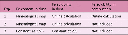
In the standard simulation (Experiment 1), spatially varying Fe solubilities for both mineral dust and combustion aerosols are used, considering different degrees of atmospheric processing in Fe-containing aerosols. In addition to the standard simulation, two experiments are performed with different assumptions of the atmospheric sources of Fe and transformation from relatively insoluble Fe to DFe for mineral dust (Table 1). To illustrate the role of combustion sources, Experiment 2 considers spatially varying solubility for mineral dust only, neglecting the combustion sources. Most ocean biogeochemistry models assume both the mass fraction and solubility of Fe in mineral dust to be constant. To quantify the effect of spatially varying solubility relative to constant solubility, we run the ocean biogeochemistry models with a uniform Fe content (3.5%) and Fe solubility (2%) for mineral dust only in Experiment 3.
Summary of sensitivity simulations performed for atmospheric input
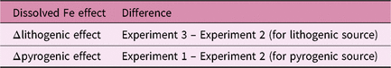
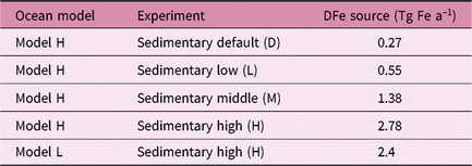
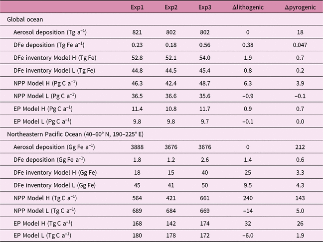
We estimate the effects of atmospheric DFe inputs of mineral dust and combustion aerosols on DFe in seawater, NPP and EP by subtracting Experiment 2 from Experiment 3 and Experiment 1 from Experiment 2, respectively (Table 2). The differences between experiments 3 and 2 are mainly caused by the differences in Fe solubility for lithogenic source in addition to those in Fe content, because the variability in Fe solubility is much larger than Fe content. The differences between experiments 1 and 2 are mainly caused by the additional DFe input by pyrogenic source, since scavenging onto pyrogenic particles is negligibly small. In Section 4.5, the difference caused by change in lithogenic source is referred to as Δlithogenic effect, and that caused by change in pyrogenic source as Δpyrogenic effect. Efficiency (η) describes how the change in DFe source affects marine productivity, and is calculated for lithogenic (pyrogenic) source by dividing Δlithogenic (Δpyrogenic) NPP or EP by Δlithogenic (Δpyrogenic) DFe deposition. Additionally, sensitivity simulations are carried out to examine how the variability of DFe sedimentary input affects η of NPP or EP in terms of additional DFe deposition fluxes with Model H (Table 3). The annual sedimentary source flux is increased from 0.27 Tg Fe a−1 in the standard run (D), to 0.55, 1.38 and 2.78 Tg Fe a−1 in the three sensitivity simulations of low (L), middle (M) and high (H) cases, respectively. To maintain a comparable NPP to the standard run, the scavenging rate for organic particles is increased accordingly in each sensitivity run.
Summary of effects of atmospheric DFe input on ocean biogeochemistry
Summary of sensitivity simulations performed for sedimentary sources
3.d. Dissolved Fe concentrations in aerosols and seawater
Measuring DFe in aerosols involves releasing DFe from the surface of the particles into solutions that typically represent either rain- (i.e. wet deposition) or seawater (i.e. dry deposition). Subsequently, the aerosol extracts are commonly passed through 0.2 or 0.45 μm filters to measure DFe and TFe, separately. Indirectly, Fe solubility is determined by dividing DFe by TFe (i.e. DFe/TFe). A global dataset of aerosol measurements shows an increase in Fe solubility with a decrease in TFe concentration (Baker & Jickells, Reference Baker and Jickells2006; Sholkovitz et al., Reference Sholkovitz, Sedwick, Church, Baker and Powell2012). However, the inverse relationship between the Fe solubility versus TFe may be an artefact of plotting two variables against each other that are not independent (TFe is used to calculate Fe solubility) (Meskhidze et al. Reference Meskhidze, Völker, Al-Abadleh, Barbeau, Bressac, Buck, Bundy, Croot, Feng, Ito, Johansen, Landing, Mao, Myriokefalitakis, Ohnemus, Pasquier and Yein press). To evaluate the ability of the IMPACT model to reproduce the observed distributions of DFe aerosol concentrations near the surface over the oceans, the model results are compared with available observations over the North Atlantic (Baker & Jickells, Reference Baker and Jickells2006; Baker et al. Reference Baker, French and Linge2006, Reference Baker, Adams, Bell, Jickells and Ganzeveld2013; Buck et al. Reference Buck, Landing and Resing2010; Powell et al. Reference Powell, Baker, Jickells, Bange, Chance and Yodle2015; Longo et al. Reference Longo, Feng, Lai, Landing, Shelley, Nenes, Mihalopoulos, Violaki and Ingall2016; Achterberg et al. Reference Achterberg, Steigenberger, Marsay, Lemoigne, Painter, Baker, Connelly, Moore, Tagliabue and Tanhua2018; Shelley et al. Reference Shelley, Landing, Ussher, Planquette and Sarthou2018) and North Pacific (Buck et al. Reference Buck, Landing, Resing and Lebon2006, Reference Buck, Landing and Resing2013). A total of 277 observations of TFe and 396 measurements of DFe over the oceans have been used in this study. We also compare our model results with specific cruises GA02 in 2010 (April 2–July 4; Achterberg et al. Reference Achterberg, Steigenberger, Marsay, Lemoigne, Painter, Baker, Connelly, Moore, Tagliabue and Tanhua2018), GA03 in 2010 (October 15–November 2) and 2011 (November 7– December 9) (Shelley et al. Reference Shelley, Landing, Ussher, Planquette and Sarthou2018) and IOC in 2002 (May 2–June 3; Buck et al. Reference Buck, Landing, Resing and Lebon2006).
It is problematic to validate model results with observations of DFe deposition in the open ocean through direct sampling, due to highly episodic rain events. Traditionally, dry deposition flux of aerosol DFe is derived from a deposition velocity and DFe concentrations in aerosols, which are sampled from shipboard during the cruise period. However, the short-term dry deposition estimate could substantially differ from long-term estimate, given the sporadic nature of dust events. In contrast, long-term dust deposition flux could be indirectly estimated, based on dissolved aluminium (DAl) concentration in the surface water, assuming that the dust is the major source of DAl to the ocean (Measures et al. Reference Measures, Brown and Vink2005). However, these estimates inherently include other sources, such as coastal inputs from the surrounding continental shelves and physical advection of surface water from other regions (Hatta et al. Reference Hatta, Measures, Wu, Roshan, Fitzsimmons, Sedwick and Morton2015; Measures et al. Reference Measures, Hatta, Fitzsimmons and Morton2015).
Measurements of reference samples from an international study of the marine biogeochemical cycles of trace elements and their isotopes (GEOTRACES) programmes ensure a consistent and comparable global dataset for trance elements such as Fe in the ocean (Rijkenberg et al. Reference Rijkenberg, Middag, Laan, Gerringa, van Aken, Schoemann, de Jong and de Baar2014; Hatta et al. Reference Hatta, Measures, Wu, Roshan, Fitzsimmons, Sedwick and Morton2015; Nishioka & Obata, Reference Nishioka and Obata2017). The results from the two ocean biogeochemistry models are compared with specific observations over the North Atlantic (Rijkenberg et al. Reference Rijkenberg, Middag, Laan, Gerringa, van Aken, Schoemann, de Jong and de Baar2014; Hatta et al. Reference Hatta, Measures, Wu, Roshan, Fitzsimmons, Sedwick and Morton2015) and North Pacific (Brown et al. Reference Brown, Landing and Measures2005; Nishioka & Obata, Reference Nishioka and Obata2017). A total of 246 observations of DFe in the upper 50 m at 112 locations have been used in this study. DFe in the models are averaged over the months of the sampling period and interpolated at the depths of the sampling. A mixed-layer depth of 50 m is assumed in this study, based on the measurements ranging from 28 m to 61 m along the GA03 (Hatta et al. Reference Hatta, Measures, Wu, Roshan, Fitzsimmons, Sedwick and Morton2015). The average concentrations and the standard deviations of model estimates and measurements are calculated from surface data and vertical profiles at the sampling locations.
4. Results and discussion
4.a. Comparison with observational data of dissolved Fe in aerosols
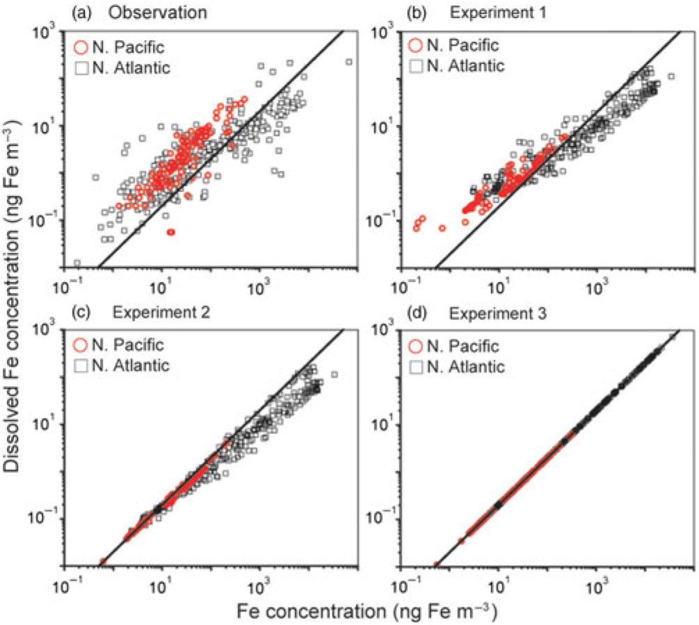
We compare our modelled concentrations of TFe and DFe in aerosols with observations over the North Atlantic (Baker & Jickells, Reference Baker and Jickells2006; Baker et al. Reference Baker, French and Linge2006, Reference Baker, Adams, Bell, Jickells and Ganzeveld2013; Buck et al. Reference Buck, Landing and Resing2010; Powell et al. Reference Powell, Baker, Jickells, Bange, Chance and Yodle2015; Longo et al. Reference Longo, Feng, Lai, Landing, Shelley, Nenes, Mihalopoulos, Violaki and Ingall2016; Achterberg et al. Reference Achterberg, Steigenberger, Marsay, Lemoigne, Painter, Baker, Connelly, Moore, Tagliabue and Tanhua2018; Shelley et al. Reference Shelley, Landing, Ussher, Planquette and Sarthou2018) and North Pacific (Buck et al. Reference Buck, Landing, Resing and Lebon2006, Reference Buck, Landing and Resing2013) (Fig. 2). Overall, only the simulation for Experiment 1 reproduces both the lower DFe concentration at higher TFe concentration over the North Atlantic and the higher DFe concentration at lower TFe concentration over the oceans (Fig. 2b). The difference between Experiment 3 and observations (Fig. 2a, d) indicates that the model with a constant Fe solubility of 2% overestimates DFe near the source regions of mineral dust. On the other hand, the difference between Experiment 2 and observations (Fig. 2a, c) suggests that the model without combustion sources underestimates the higher DFe concentrations in both ocean basins. This is particularly substantial in the North Pacific, since a combustion source from the East Asia can be a significant DFe source, compared with a sporadic mineral dust source (Ito, Reference Ito2015; Ito et al. Reference Ito, Myriokefalitakis, Kanakidou, Mahowald, Scanza, Hamilton, Baker, Jickells, Sarin, Bikkina, Gao, Shelley, Buck, Landing, Bowie, Perron, Guieu, Meskhidze, Johnson, Feng, Kok, Nenes and Duce2019).
Relationship between total Fe and dissolved Fe concentrations (ng Fe m−3) in aerosols for (a) observation, (b) Experiment 1, (c) Experiment 2 and (d) Experiment 3 over the North Pacific (red circles) and the North Atlantic (black squares). The solid black line shows a linear trend with a constant Fe solubility of 2%.
4.b. Comparison along North Atlantic (GA02 and GA03) and North Pacific (IOC 2002 and GP02) cruises
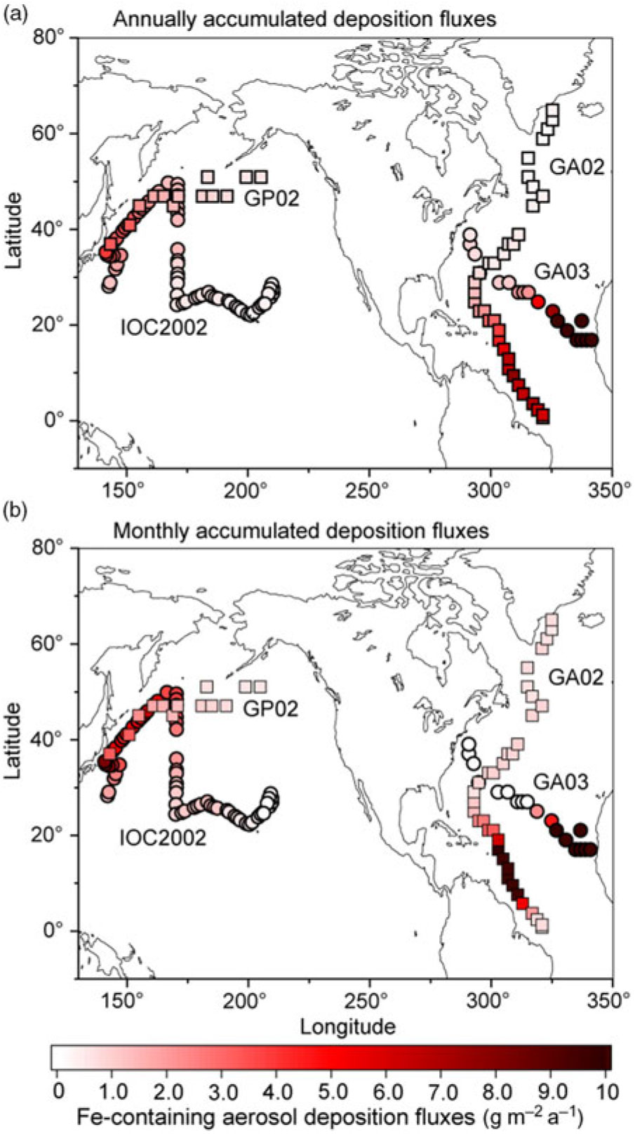
We compare our model results with specific cruises GA02 (Rijkenberg et al. Reference Rijkenberg, Middag, Laan, Gerringa, van Aken, Schoemann, de Jong and de Baar2014; Achterberg et al. Reference Achterberg, Steigenberger, Marsay, Lemoigne, Painter, Baker, Connelly, Moore, Tagliabue and Tanhua2018), GA03 (Hatta et al. Reference Hatta, Measures, Wu, Roshan, Fitzsimmons, Sedwick and Morton2015; Shelley et al. Reference Shelley, Landing, Ussher, Planquette and Sarthou2018), IOC 2002 (Brown et al. Reference Brown, Landing and Measures2005; Buck et al. Reference Buck, Landing, Resing and Lebon2006) and GP02 (Nishioka & Obata, Reference Nishioka and Obata2017). The atmospheric Fe-containing aerosol deposition fluxes are contoured to illustrate the geographical distribution of the gradients along the cruise tracks (Fig. 3a). Annually averaged dust deposition fluxes decrease from 77 g m−2 a−1 in the eastern North Atlantic near the Saharan dust source to 0.57 g m−2 a−1 in the western North Atlantic along the GA03. At the latter locations, the model estimates are significantly lower than the calculated dust deposition from DAl concentration in seawater (3.61 g m−2 a−1) (Measures et al. Reference Measures, Hatta, Fitzsimmons and Morton2015). The latter value does not represent a geographically static region as in the former values, but reflects a c. 5-year running average of dust input into the surface water as it moves from the south due to substantial advection of surface water in the Gulf Stream (Measures et al. Reference Measures, Hatta, Fitzsimmons and Morton2015). This is consistent with the higher simulated dust deposition fluxes (up to 7.73 g m−2 a−1) into the Caribbean Sea along the GA02. The simulated dust deposition fluxes decrease from 3.9 g m−2 a−1 in the western North Pacific near Japan to 0.23 g m−2 a−1 in the central North Pacific along the IOC 2002, which are in reasonable agreement with those based on the measurement of Al concentration in seawater (Measures et al. Reference Measures, Brown and Vink2005). The annually averaged dust deposition fluxes are also calculated from monthly accumulated deposition fluxes during the cruise periods to illustrate seasonal variability in dust (Fig. 3b). The dust deposition fluxes near Japan in spring (up to 8.12 g m−2 a−1 along the IOC 2002) are significantly larger than those in summer (0.26 g m−2 a−1 at the westernmost location along the GP02).
Annually averaged deposition fluxes of atmospheric Fe-containing aerosol along the cruise tracks from the IMPACT model. The locations of the four cruises are taken from GA02 (squares) during April–July (Achterberg et al. Reference Achterberg, Steigenberger, Marsay, Lemoigne, Painter, Baker, Connelly, Moore, Tagliabue and Tanhua2018), GA03 (circles) during October–November (Shelley et al. Reference Shelley, Landing, Ussher, Planquette and Sarthou2018), IOC 2002 (circles) during May–June (Buck et al. Reference Buck, Landing, Resing and Lebon2006) and GP02 (squares) during August–September (Nishioka & Obata, Reference Nishioka and Obata2017). Estimates from (a) annually accumulated and (b) monthly accumulated deposition fluxes during the cruises.
The comparison of the calculated and measured DFe in aerosols indicates that Experiment 1 captures the DFe observations reasonably well (Fig. 4a–c). Experiments 2 and 3 underestimate the aerosol DFe influenced by anthropogenic sources in the western North Atlantic near the North American continent (Fig. 4b), while Experiment 3 overestimates DFe concentration over the tropical and subtropical Atlantic downwind from the North African dust plume (Fig. 4a, b). The model underestimates DFe concentrations in aerosols over south Greenland, which are above background levels and probably resulted from the Eyjafjallajökull 2010 eruption. The IMPACT model does not consider aerosol emissions from the specific volcanic events, and therefore shows good agreement with the observations for samples which are not affected by the volcanic ash in the region (Achterberg et al. Reference Achterberg, Steigenberger, Marsay, Lemoigne, Painter, Baker, Connelly, Moore, Tagliabue and Tanhua2018). Along IOC 2002, high DFe in aerosols during short-term events of Asian dust over east Japan might be captured by the daily averaged estimates of DFe in the model but not by the monthly mean, given the sporadic nature of dust events (Fig. 4c) (Ito et al. Reference Ito, Myriokefalitakis, Kanakidou, Mahowald, Scanza, Hamilton, Baker, Jickells, Sarin, Bikkina, Gao, Shelley, Buck, Landing, Bowie, Perron, Guieu, Meskhidze, Johnson, Feng, Kok, Nenes and Duce2019).
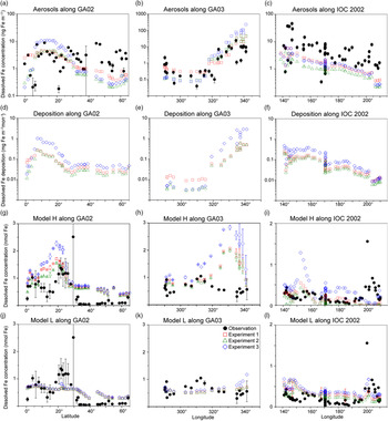
Comparison of monthly averaged estimates from Experiment 1 (red squares), Experiment 2 (green triangles) and Experiment 3 (blue diamonds) with field data (black circles) in the North Atlantic and the North Pacific. (a–c) Atmospheric DFe concentration in aerosols. (d–i) DFe deposition and DFe concentrations in the surface ocean in Model H. Model L shares the same DFe deposition as Model H. (j–l) DFe concentrations in the surface ocean in Model L. The measurements of aerosols are taken from GA02 (Achterberg et al. Reference Achterberg, Steigenberger, Marsay, Lemoigne, Painter, Baker, Connelly, Moore, Tagliabue and Tanhua2018), GA03 (Shelley et al. Reference Shelley, Landing, Ussher, Planquette and Sarthou2018) and IOC 2002 (Buck et al. Reference Buck, Landing, Resing and Lebon2006). The measurements of seawater DFe are taken from the same cruises (GA02, Rijkenberg et al. Reference Rijkenberg, Middag, Laan, Gerringa, van Aken, Schoemann, de Jong and de Baar2014; GA03, Hatta et al. Reference Hatta, Measures, Wu, Roshan, Fitzsimmons, Sedwick and Morton2015; IOC 2002, Brown et al. Reference Brown, Landing and Measures2005). The error bars in (g–l) represent the variability for the depth in the upper 50 m (±σ).
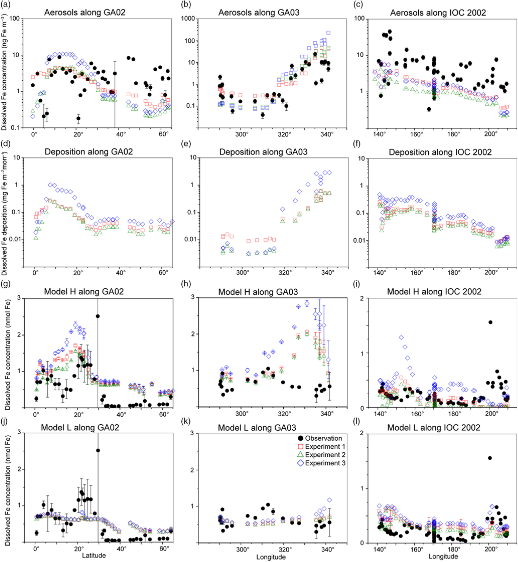
The atmospheric deposition flux (Fig. 4f) is decoupled from DFe concentration in aerosols along IOC 2002 (Fig. 4c). This result reflects the greater level of atmospheric processing of aerosols at lower altitudes because of the more acidic air pollutants near the ground surface. The relatively high Fe solubility was derived from shipboard aerosol sampling (2.5 ± 1.2% in seawater leaches north of 45° N) for mineral dust, which could be transported at higher altitudes and delivered into the ocean via rainout. Use of the high Fe solubility of 2% for mineral dust in Experiment 3 would therefore lead to overestimations of DFe supply in the North Pacific Ocean. The shipboard-sampled aerosol represents the state of the atmosphere over daily timescales. In contrast, DAl in seawater is assumed to represent a moving average of dust input over 5 years as a result of its longer residence time in seawater than aerosols. This means that a deposition flux has been estimated (Brown et al. Reference Brown, Landing and Measures2005) based on the measurement of Fe concentration in aerosols (Buck et al. Reference Buck, Landing, Resing and Lebon2006) that is about five times larger than that based on Al concentration in seawater (Measures et al. Reference Measures, Brown and Vink2005), even when the dry deposition flux of aerosols was compared with total (dry + wet) deposition flux. As a result, the annually averaged atmospheric dust deposition fluxes (Fig. 3) are in good agreement (0.1–0.5 g m−2 a−1 in the eastern part of the cruise, excluding the vicinity of the Hawaiian Islands) with those based on the measurement of Al concentration in seawater (Measures et al. Reference Measures, Brown and Vink2005), although the monthly averaged DFe concentration in aerosols over the central North Pacific is significantly underestimated (Fig. 4c).
In addition to the atmospheric input of DFe, surface DFe concentrations in the two ocean biogeochemistry models along the four cruises are compared with observations in the upper 50 m (Figs 4, 5). The observations of DFe in the surface ocean show a N–S gradient along GA02 (Fig. 4g, j), relatively high DFe along GA03 under the Saharan dust plume and near the North American continent (Fig. 4h, k), and relatively low DFe along IOC 2002 with a peak close to the eastern end of the cruise (Fig. 4i, l). The observed peak of higher concentrations in the eastern end of the cruise has been attributed to fluvial runoff from the nearby islands (Measures et al. Reference Measures, Brown and Vink2005), which is not considered in either Model H or Model L. The observations of DFe along GP02 show relatively high concentration at the westernmost station near the Japanese coast (Fig. 5), while dust deposition fluxes in summer are much smaller than those during Asian dust season (Fig. 3). The western DFe-rich water has been attributed to external sedimentary DFe sources (Nishioka & Obata, Reference Nishioka and Obata2017).
Comparison of monthly averaged estimates of DFe concentrations in the surface ocean sensitivity simulations performed for sedimentary sources (Table 3) in Model H (red squares) and Model L (green triangles) with field data (black circles) in the North Pacific. The measurements of seawater DFe are taken from the GP02 (Nishioka & Obata, Reference Nishioka and Obata2017). The error bars represent the variability for the depth in the upper 50 m (±σ).

DFe in Model H shows a large variability of DFe (0.53 ± 0.52 nM in Experiment 1) with a similar range of measurements in the North Pacific, but is clearly overestimated along the two Atlantic cruises. Along GA02, the standard simulation (Experiment 1) basically follows the pattern of deposition (Fig. 4d), increasing from the equator to 20° N, decreasing to 30° N and then varying within a small range between 0.5 and 0.75 nM (Fig. 4g). All three experiments reproduce the N–S gradient found in the measurements, reflecting a strong Fe source in the tropical and subtropical North Atlantic, which is consistent with the strong correlation between the measured sea surface DFe and DAl (Rijkenberg et al. Reference Rijkenberg, Middag, Laan, Gerringa, van Aken, Schoemann, de Jong and de Baar2014). Comparing the results of the three experiments, DFe mainly differs between 10° N and 25° N in the subtropical Atlantic, caused by the change in DFe deposition. DFe in Experiment 3 with a fixed Fe content and solubility is more than 1 nM higher than the measurements. The measurements show a strong decline between 10° N and 20° N assigned to biological uptake (Rijkenberg et al. Reference Rijkenberg, Middag, Laan, Gerringa, van Aken, Schoemann, de Jong and de Baar2014). In the model the decline is much weaker, and is barely discernible in Experiment 3. Several factors could contribute to this in the model. (1) The model does not take into account the riverine input of Fe, and therefore misses a source of DFe between the equator and 20° N where Fe is transported from the Amazon River plume into the surface ocean. (2) The model tends to overestimate DFe under dust plume, and this feature extends from the subtropical North Atlantic northwards to the high latitudes. However, the atmospheric deposition fluxes are significantly lower than the fluxes associated with deep winter mixing in the high-latitude North Atlantic (Achterberg et al. Reference Achterberg, Steigenberger, Marsay, Lemoigne, Painter, Baker, Connelly, Moore, Tagliabue and Tanhua2018). The possible reasons for the overestimation are explained below. (3) As well as biological uptake, scavenging onto living phytoplankton cells could also play a role in removing DFe from the surface waters (Hudson & Morel Reference Hudson and Morel1989; Pagnone et al. Reference Pagnone, Völker and Ye2019), particularly in regions with high biological production. The decline of DFe is shown to correlate well with the high surface fluorescence at c. 15° N (Rijkenberg et al. Reference Rijkenberg, Middag, Laan, Gerringa, van Aken, Schoemann, de Jong and de Baar2014). These three factors might lead to an underestimation of the variability of DFe between the equator and 20° N: the background concentration is too high due to the overestimation of the lifetime of DFe after rainfall (Baker & Croot, Reference Baker and Croot2010; Meskhidze et al. Reference Meskhidze, Hurley, Royalty and Johnson2017), and the contrast between 5 and 15° N is too small due to the missing riverine input and phytoplankton scavenging.
Along GA03, the modelled DFe (Fig. 4h) also follows the pattern of deposition which is clearly elevated under the Saharan dust plume (Fig. 4e). The model tends to overestimate DFe concentration in regions with high deposition between 320° E and 340° E, even considering lithogenic scavenging (Ye & Völker, Reference Ye and Völker2017) and a variable solubility of Fe in dust. A possible explanation is that the model does not take into account the size-segregated speciation of DFe between soluble and colloidal Fe. The latter could significantly contribute to the DFe pool along the GA03 cruise in the surface ocean where atmospheric input from mineral dust is the major source of DFe (Fitzsimmons et al. Reference Fitzsimmons, Carrasco, Wu, Roshan, Hatta, Measures, Conway, John and Boyle2015; Hatta et al. Reference Hatta, Measures, Wu, Roshan, Fitzsimmons, Sedwick and Morton2015; Measures et al. Reference Measures, Hatta, Fitzsimmons and Morton2015). It is therefore crucial for the global Fe models to consider colloid formation and the subsequent pathway of faster Fe removal via more active aggregation of colloidal Fe into particulate Fe phase than just via particle adsorption of soluble Fe (Honeyman & Santschi Reference Honeyman and Santschi1989; Ye et al. Reference Ye, Völker and Wolf-Gladrow2009). In spite of the high background concentrations of DFe in the eastern part of the transect, a decline is found in the model east of 330° E caused by high biological uptake near the African coast and scavenging by organic and lithogenic particles (Ye & Völker, Reference Ye and Völker2017). Comparing the three experiments, Experiment 3 (assuming a fixed Fe content and solubility) produces DFe up to c. 1 nM higher in the eastern part of the transect than the other two experiments. In the western part of the transect (west of 315° E), in spite of higher deposition in Experiment 1, DFe in the surface ocean is slightly lower than in Experiment 3. This decoupling of seawater DFe from DFe deposition could be caused by the difference of DFe deposition between experiments 3 and 1 in the surrounding waters of GA03 stations and the transport of water masses. Higher DAl concentrations have been measured in the Gulf Stream, which carries waters from the Caribbean Sea where a much larger amount of mineral dust is delivered from North Africa (Measures et al. Reference Measures, Hatta, Fitzsimmons and Morton2015). Ignoring the atmospheric processing, DFe in seawater is higher in the Caribbean Sea, and the inflow of water mass from the Caribbean Sea leads to an elevation of DFe in the western part of GA03 in Experiment 3.
Modelled DFe along the IOC 2002 cruise track is higher in the west and decreases towards the east (Fig. 4i), consistent with the trend of deposition (Fig. 4f). The modelled DFe of Experiment 1 (0.16 ± 0.12 nM) matches well with measured DFe (0.23 ± 0.20 nM), but Experiment 3 generates a twofold higher concentration on average (0.35 ± 0.22 nM), indicating that the solubility of Fe in the North Pacific Ocean would be severely overestimated by assuming a fixed Fe solubility of 2%. Furthermore, the overestimations of DFe from mineral dust in the seawater may imply that the atmospheric models need to consider the partitioning of DFe into Fe-organic complexes or colloidal inorganic Fe in rainwater. The latter might be formed due to less Fe-binding organic compounds in mineral aerosols (Ito & Shi, Reference Ito and Shi2016). The chemical speciation of organic ligands as well as size-segregated measurements of DFe between colloids and aqueous species in rainwater are needed in future work.
A comparison of DFe during summer months along the GP02 shows that the elevated DFe concentrations can be driven by the sedimentary input that is mixed and advected offshore (Fig. 5d), with a lesser contribution from atmospheric input (Fig. 3). Model H reproduces the relatively high DFe concentrations at the westernmost station near the Japanese coast observed in the surface layer along the GP02, regardless of the relative inputs of the sedimentary sources (Fig. 5).
Model L captures the average of DFe in the surface ocean, but shows a small variability (0.48 ± 0.17 nM in Experiment 1) compared with the measurements along the three cruises (0.44 ± 0.61 nM). The results of three experiments in most cases do not significantly differ from each other because the maximum Fe solubility in seawater is mainly controlled by the threshold of 0.6 nM. This threshold approach leads to an underestimation of relatively high DFe concentrations along GA02. Nevertheless, using the constant Fe solubility in Experiment 3, extremely large DFe deposition along the GA03 cruise near the dust source regions (Fig. 4e) leads to overestimations of DFe in the eastern North Atlantic (Fig. 4k). These overestimations are reduced in both experiments 1 and 2, which consider different degrees of atmospheric Fe processing. Model L shows an overestimation of DFe at relatively low concentrations along the IOC 2002 in the North Pacific (except the nearshore data from Hawaii), mostly because of low scavenging rates when DFe is below the threshold of 0.6 nM (Fig. 4l).
4.c. Global distribution of dissolved Fe deposition fluxes during spring
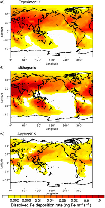
Mineral dust is the major source of aerosol DFe deposition (79%) on a global scale, compared with pyrogenic Fe-containing aerosols (Table 4). Here, we focus on the analysis of data averaged from March to May in spring when the major dust plume typically moves out from East Asia to the North Pacific. The standard simulation (Experiment 1) shows that most DFe is deposited in the North Atlantic, Arabian Sea and South Atlantic downwind of the arid and semi-arid regions of North Africa, the Middle East and Patagonia (Fig. 6a). When atmospheric processing of mineral dust is not considered, Experiment 3 overestimates deposition to most parts of the oceans such as the North Atlantic, North Pacific and Southern Ocean, and specifically to the south of Patagonia, Australia and southern Africa (Fig. 6b). Mineral dust deposited in regions far away from the dust source could have undergone intensive atmospheric processing during long-range transport. The simulated solubility can therefore be higher than 2% over the tropical and South Pacific, part of the Indian Ocean, subtropical South Atlantic and Southern Ocean. However, the total deposition is very small over these areas. When additional combustion sources are neglected, Experiment 2 underestimates the deposition flux to the North Pacific, North Atlantic and tropical oceans (Fig. 6c).
Changes in deposition, dissolved iron (DFe) inventory, net primary production (NPP) and export production (EP) in the three experiments conducted with two ocean biogeochemistry models
Deposition fluxes of dissolved Fe (ng Fe m−2 s−1) from dust and combustion sources to the oceans during spring (March–May). (a) Spatial distribution of DFe for Experiment 1. (b) Differences (Experiment 3 – Experiment 2) for lithogenic source (Δlithogenic). (c) Differences (Experiment 1 – Experiment 2) for pyrogenic (Δpyrogenic) source. Some areas shaded in white contain small negative values.

4.d. Global distribution of dissolved Fe in the surface ocean during spring
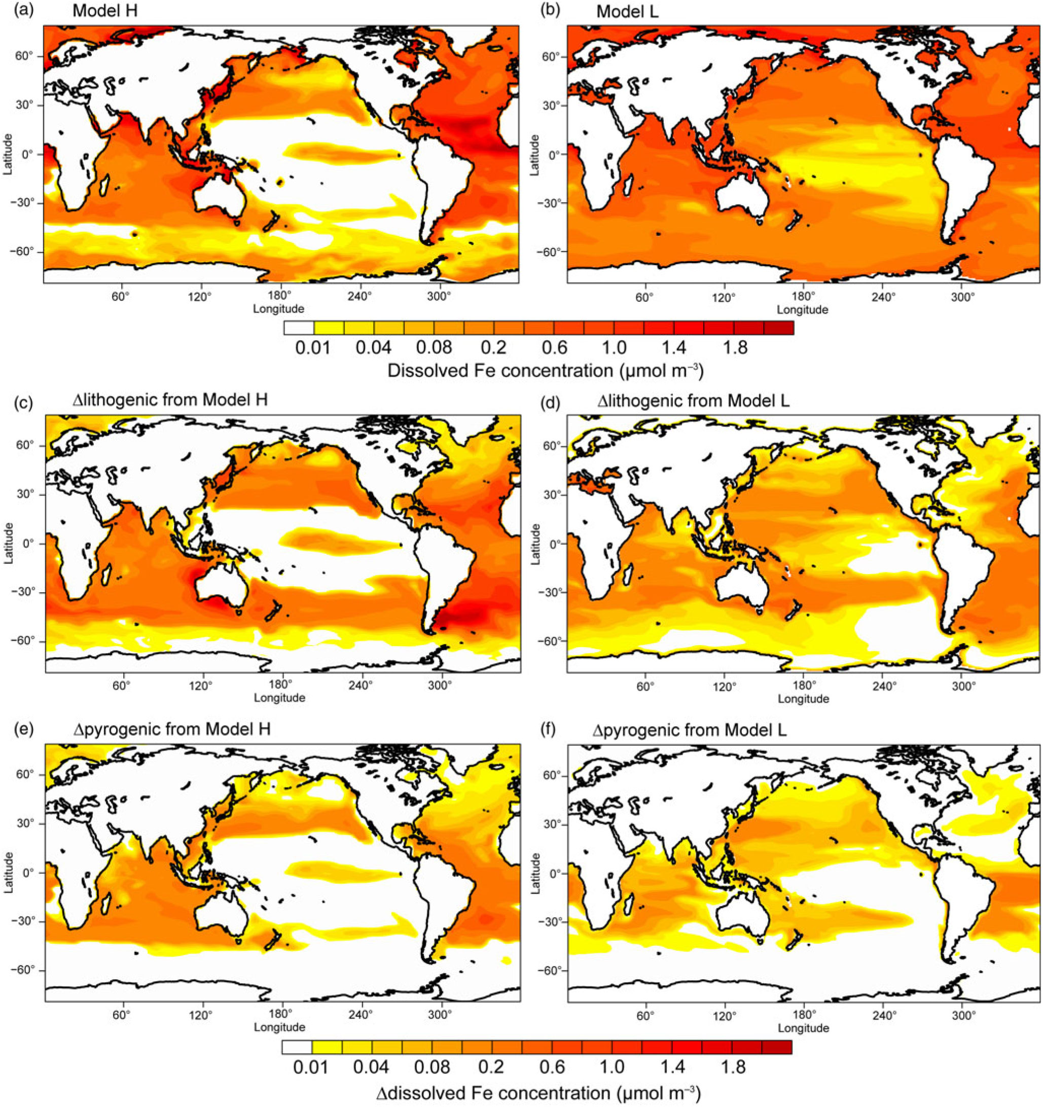
Results from Model H show a similar spatial pattern to Model L, but a higher sensitivity of DFe to changes in atmospheric deposition (Table 4 and Fig. 7); this is partly due to the faster Fe scavenging on sinking particles when DFe concentrations exceed 0.6 nM in Model L (Moore et al. Reference Moore, Doney and Lindsay2004). When atmospheric processing of mineral dust is not considered, both models produce higher DFe concentrations, mainly in regions close to dust source regions but also in large areas in the subtropical North and South Pacific (Fig. 7c, d). When additional combustion sources are considered simulated DFe in both models becomes higher (Fig. 7e, f), particularly in the tropical and subtropical South Atlantic, the subtropical North Pacific and Indian Ocean.
Dissolved Fe concentration (μmol m−3) in the surface oceans during spring. (a, b) Spatial distribution of DFe for Experiment 1. (c, d) Differences (Experiment 3 – Experiment 2) for lithogenic source (Δlithogenic). (e, f) Differences (Experiment 1 – Experiment 2) for pyrogenic source (Δpyrogenic).
4.e. Effects on marine primary production and export production
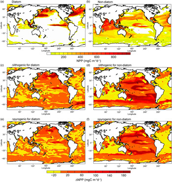
Each phytoplankton functional type responds differently to the imposed changes in DFe deposition, according to their physiological nature. Large open-ocean diatoms are mostly less efficient in nutrient uptake compared with small non-diatom phytoplankton (Sunda & Huntsman, Reference Sunda and Huntsman1997). Diatoms are assumed to have a requirement for silicate (Si) (no such requirement for non-diatoms) and a higher half-saturation constant for N uptake (i.e. 1.0 v. 0.55 mmol N m−3) and Fe uptake (i.e. 0.12 v. 0.02 μmol Fe m−3) compared with non-diatoms (Sunda & Huntsman, Reference Sunda and Huntsman1997). Model H also takes into account the fact that diatoms are more resistant to grazing and can grow better under conditions of low light. The geographical distribution of NPP for diatoms therefore shows lower production in most Fe-limited oceanic regions such as the subtropical gyres during spring (Fig. 8a). At the same time, diatoms have a larger maximum growth rate (i.e. 3.5 v. 3.0 day−1). Fe inputs from the atmosphere and upwelling of nutrient-rich water could therefore fuel the spring blooms of diatoms in high-nutrient–low-chlorophyll (HNLC) regions such as the subarctic North Atlantic, North and equatorial Pacific. On the other hand, relatively high NPP for non-diatoms is estimated in Si-limited regions of diatoms such as the tropical Indian Ocean, where enough DFe is supplied (Fig. 8b). In regions where N is the predominantly limiting nutrient, for example the Atlantic Ocean (Fig. 8b), small phytoplankton outcompetes diatom by its lower half saturation constant for N uptake.
Net primary production (NPP) (mg C m−2 day−1) for diatoms and non-diatoms from Model H in the oceans during spring. (a, b) Spatial distribution of NPP for Experiment 1. (c, d) Differences (Experiment 3 – Experiment 2) for lithogenic source (Δlithogenic). (e, f) Differences (Experiment 1 – Experiment 2) for pyrogenic source (Δpyrogenic).

To illustrate the magnitude of biological response to change in atmospheric DFe sources, we compared Δlithogenic and Δpyrogenic NPP from Model H. By assuming a constant solubility of 2% (Fig. 8c, d) or adding the pyrogenic source (Fig. 8e, f), NPP clearly increases in regions with intense Fe-limitation (e.g. the Pacific Ocean and Southern Ocean) and decreases in regions limited by macronutrients, although DFe input is larger (e.g. low latitudes in the Atlantic Ocean and Arabian Sea). More macronutrients are therefore consumed in Fe-limiting regions, and less can be transported to other ocean regions. This causes the decrease of NPP in N-limiting regions, particularly for non-diatoms. The Pacific Ocean is generally Fe-limiting in the model; however, the response pattern of NPP does not simply follow the pattern of enhanced DFe concentration. This is explained by competition for Fe and macronutrients between the two phytoplankton groups: diatoms and non-diatoms. Diatoms demand much more DFe uptake than non-diatoms and are therefore out-competed if DFe supplies decrease. Surrounding the areas of enhanced diatoms, excess nutrients become available for non-diatoms and support higher production. The net change of NPP is therefore controlled by both nutrient supply and community composition of phytoplankton.
Table 4 gives an overview of annually accumulated deposition of aerosols and DFe inventory from lithogenic and pyrogenic sources, and their effects on NPP and EP in the three experiments, for the global ocean and northeastern Pacific (40–60° N, 190–225° E), respectively. Global DFe input from dust (0.18–0.56 Tg Fe a−1) and DFe inventory (45–54 Tg Fe) are within the range (0.08–1.81 Tg Fe a−1 and 27–70 Tg Fe, respectively) of 13 global Fe models compared in the framework of the iron model intercomparison project (FeMIP) (Tagliabue et al. Reference Tagliabue, Aumont, Death, Dunne, Dutkiewicz, Galbraith, Misumi, Moore, Ridgwell, Sherman, Stock, Vichi, Völker and Yool2016).
Despite the much larger Δlithogenic DFe deposition (0.38 Tg Fe a−1) than Δpyrogenic (0.05 Tg Fe a−1), we find comparable Δlithogenic and Δpyrogenic NPP of 6.3 and 3.9 Pg C a−1, respectively, in Model H. The parameters Δlithogenic and Δpyrogenic EP in Model H are also similar (0.9 and 0.7 Pg C a−1). Response of marine productivity to atmospheric DFe input depends on the magnitude of Fe-limitation of phytoplankton growth. Lithogenic and pyrogenic Fe deposition fluxes are distributed over different regions of the oceans. Regions that receive the most substantial amounts of pyrogenic Fe are the Pacific and Southern oceans, where phytoplankton growth is strongly limited by Fe. New production can therefore be stimulated by additional input of pyrogenic Fe, resulting in a more efficient increase in NPP (η = 85) and EP (η = 14) than lithogenic Fe on a global scale (Fig. 9). In contrast, phytoplankton growth is not predominantly limited by Fe in most regions receiving the majority of the lithogenic DFe, such as the subtropical North Atlantic Ocean and Arabian Sea. At the same time, phytoplankton growth at lower latitudes in the Pacific Ocean is still predominantly limited by Fe, even in Experiment 3. Change in lithogenic source therefore still has a positive effect on marine productivity, but a low efficiency for NPP (η = 16) and EP (η = 2) compared with a pyrogenic source (Fig. 9).
Efficiency (η) of ΔNPP/Δdeposition and ΔEP/Δdeposition for different sedimentary and atmospheric inputs in Model H and Model L. (a, b) ΔNPP/Δdeposition and ΔEP/Δdeposition in the global ocean. (c, d) ΔNPP/Δdeposition and ΔEP/Δdeposition in the northeastern Pacific Ocean.

Globally, Model L shows little and negative Δlithogenic NPP (–2.6%) and EP (–1.5%), even although global DFe deposition from mineral dust increases from 0.18 Tg Fe a−1 to 0.56 Tg Fe a−1 by a factor of 3. The spatial reorganization in NPP is responsible for the small net change in global NPP (Aumont et al. Reference Aumont, Maier-Reimer, Blain and Monfray2003; Sarmiento et al. Reference Sarmiento, Gruber, Brzezinski and Dunne2004; Tagliabue et al. Reference Tagliabue, Bopp and Aumont2008). NPP is enhanced in the Southern Ocean assuming a constant Fe solubility of the lithogenic deposition, because the simulated Fe solubility in mineral dust is much lower than the prescribed value of 2%. This enhancement of NPP increases the utilization of macronutrients, which are exported into the deep water. Since Model L does not consider the return path of macronutrients from the sediments, the depleted macronutrients reduce NPP in the macronutrient-limited low latitudes. A similar mechanism also occurs for Δpyrogenic NPP (–0.3%) and EP (0.1%) in the global ocean, as the elevated NPP in the northeastern Pacific is balanced by the reduced NPP at lower latitudes.
In the northeastern Pacific, Model H shows a more intensive increase in DFe inventory than Model L by both Δlithogenic and Δpyrogenic, while Model L has a much larger DFe inventory (lower part of Table 4). This can be partly explained by the ratio of atmospheric to sedimentary input: 1:1.2 in Model H versus 1:10 in Model L. We examine the effects of sedimentary sources on η of NPP or EP to the additional DFe deposition (Fig. 9). The results clearly demonstrate higher η of NPP and EP to the combustion aerosols than to mineral dust, regardless of the relative inputs of the sedimentary sources in Model H. In contrast to the global ocean, lithogenic Fe can stimulate NPP in Model H with a high and comparable efficiency to pyrogenic Fe in the northeastern Pacific. A key factor here is the seasonality. Asian dust delivers the majority of DFe in spring when marine biological activity is high but often limited by Fe. Thus, both the spatial distribution and temporal variation of atmospheric DFe sources affect their efficiency in changing NPP.
5. Conclusions
Human activity perturbs both the sources of Fe and the effects of atmospheric processing on the bioavailability of Fe delivered to the ocean. The IMPACT model simulates less Fe emissions from pyrogenic sources, but faster photochemical transformation for pyrogenic Fe-containing aerosols and therefore more DFe deposition to the HNLC regions. The two ocean biogeochemistry models receive DFe from the atmosphere and simulate the Fe cycle and associated biogeochemical cycles of other nutrients. The more detailed model with higher sensitivity to change in the atmospheric input of DFe (Model H) suggests that pyrogenic Fe-containing aerosols stimulate NPP and EP more efficiently than lithogenic aerosols, relative to the smaller Fe amount in pyrogenic deposition, because biological production in oceanic regions receiving most of the pyrogenic deposition would be predominantly limited by DFe if ignoring the pyrogenic source of DFe.
The two ocean biogeochemistry models show substantially different magnitudes of response to the atmospheric input of DFe, depending on the parameterization of DFe sinks as well as assumptions about other DFe sources. Model H uses variable ligand-binding capacity and describes scavenging as a function of DFe and settling particle concentrations, which allows higher variability and sensitivity of DFe to its sources. Moreover, the variable (and in many cases higher) binding capacity of ligands keep more Fe in the dissolved form, and therefore available for scavenging and biological uptake in the model. The trend of overestimation of DFe in high-deposition regions indicates that parameterization of scavenging loss becomes critical to shaping the pattern of DFe distribution. On the other hand, Model L still uses the threshold approach by assuming the presence of Fe-binding ligands ubiquitously. That yields a modelled DFe that is in good agreement with the average concentration of DFe measured in the surface ocean, but suppresses the variability and therefore results in the low sensitivity of DFe to changes in its sources. Furthermore, the models use the same atmospheric input of DFe but substantially different sedimentary source strengths. Using Model H, we examined the sensitivity to the sedimentary input of DFe by increasing the sedimentary default (D) by a factor of 2, 6 and 12 compared with that used in the default version of Model H. The results suggest that our conclusion of higher sensitivity of NPP to the change in combustion aerosols than to mineral dust is robust, regardless of the relative sedimentary source inputs.
These results highlight that it is not only the atmospheric processing and deposition of Fe, but also the capacity of the ocean to keep deposited DFe available for biology, that are key to understanding the role of atmospheric deposition to the ocean. Knowledge of chemical speciation of Fe, such as size-segregated measurements of DFe in both rain- and seawater, is needed in conjunction with concentrations and complexing capacities of organic ligands. Solubility of Fe in the surface ocean may also be affected by certain organic ligands supplied via atmospheric deposition (Meskhidze et al. Reference Meskhidze, Hurley, Royalty and Johnson2017). By incorporating Fe-containing aerosols with organic ligands emanating from natural and anthropogenic sources in the assessment of atmospheric fluxes of DFe to the surface ocean, we can improve our understanding of the effect of human perturbations on DFe supply, especially in HNLC regions. Since atmospheric DFe input plays a key role in prediction of marine biogeochemical properties (e.g. oxygen, primary production; Park et al. Reference Park, Stock, Dunne, Yang and Rosati2019; Yamamoto et al. Reference Yamamoto, Abe-Ouchi, Ohgaito, Ito and Oka2019), the effect of anthropogenic Fe-containing aerosols on the marine ecosystem should be explored for marine resource management with Earth system models in the future.
Acknowledgements
Support for this research was provided to AI, AY, MW and MNA by the Integrated Research Program for Advancing Climate Models (MEXT). The research work by YY was supported by the project PalMod (PaleoModeling, Federal Ministry of Education and Research Germany (BMBF) 01LP1505C). AI acknowledges financial support from the Japan Society for the Promotion of Science (JSPS) grant no. JP16K00530. Numerical simulations were performed using the Hewlett Packard Enterprise (HPE) Apollo at the Japan Agency for Marine-Earth Science and Technology (JAMSTEC) and Nippon Electric Company (NEC) supercomputer (SX-ACE) at Alfred Wegener Institute, respectively. The Modern Era Retrospective Analysis for Research and Applications, version 2 (MERRA-2) were provided by the Global Modeling and Assimilation Office (GMAO) at NASA Goddard Space Flight Center.


 Open access