


1. Introduction
The escalating global dependence on single-use plastic packaging has generated significant environmental impacts, thereby necessitating a profound and systemic reconfiguration of the food production systems and the current packaging model (Reference Geyer, Jambeck and LawGeyer et al., 2017). In response to this, new packaging regulations and policies are emerging worldwide. In the European context, exigent legislative instruments have been introduced, including the Packaging and Packaging Waste Directive (PPWD) and the Packaging and Packaging Waste Regulation (PPWR). These policies are expressly intended to limit the environmental impact of packaging waste, setting clear targets for both reduction and reuse (European Commission, 2022).
Within the circular economy (CE) framework, reuse is prioritized as the most effective strategy for retaining the material value of packaging, taking priority over recycling and recovery in the waste hierarchy (Reference EuropéenParlement Européen, 2008). However, the transition from linear single-use models to circular reuse packaging systems is inherently complex, requiring consideration of multiple, interrelated variables for their design to effectively reduce environmental impacts.
From a life cycle assessment (LCA) perspective, reuse loops are primarily driven by the uncertainty of reverse logistics, where the environmental issue of transporting heavier, empty crates in the return trip can outweigh benefits if return distances are not minimized (Reference Accorsi, Cascini, Cholette, Manzini and MoraAccorsi et al., 2014; Reference Levi, Cortesi, Vezzoli and SalviaLevi et al., 2011). Environmental impacts are heavily dependent on the assumed number of rotations (trip rates) and breakage rates, which determine the critical “break-even point” against single-use cardboard (Reference Koskela, Dahlbo, Judl, Korhonen and NiininenKoskela et al., 2014; Reference Singh, Chonhenchob and SinghSingh et al., 2006). Furthermore, the use phase introduces significant variability through industrial washing and sanitization processes, which consume substantial water and energy resources often exceeding production impacts (Reference Accorsi, Cascini, Cholette, Manzini and MoraAccorsi et al., 2014). Finally, the impact of end-of-life packaging remains difficult to estimate due to the wide range of divergent assumptions regarding closed-loop recycling versus downcycling, which can alter their own environmental performance and that of the loops in which they are used (Reference Tua, Biganzoli, Grosso and RigamontiTua et al., 2019). Consequently, the environmental performance of reuse loop systems depends heavily on the choices made during their design as even a small inefficiency in loop operations can undermine environmental outcomes (Reference Coelho, Corona, ten Klooster and WorrellCoelho et al., 2020). For this reason, environmental assessment methods capable of rapidly exploring multiple design scenarios are essential, ensuring that conclusions remain robust across the wide range of operational conditions that can arise in real systems.
In this context, the use of full LCA studies to support the design of reuse packaging loops is not practical, as they require substantial time and detailed data that are rarely available during early design stages. To manage the environmental assessment of reuse loops, rather than developing a full LCA analysis itself, it is possible to apply simplification methods to reduce the required data and time (Reference Suppipat, Chotiratanapinun, Teachavorasinskun and HuSuppipat et al., 2023). These simplifications are context-specific approximations, and their validity is therefore limited to the specific system for which they are built. In general, Global Sensitivity Analysis (GSA) is the most widely adopted simplification method. GSA enables the identification of the most influential input variables of a model, by quantifying how much of the environmental impact variance can be explained by the variation of each input. It has been extensively applied to simplify energy systems (Reference Di Lullo, Gemechu, Oni and KumarDi Lullo et al., 2020; Reference Douziech, Ravier, Jolivet, Pérez-López and BlancDouziech et al., 2021; Reference Gibon and Hahn MenachoGibon & Hahn Menacho, 2023; Reference Paulillo, Cui, Brown, Striolo and LettieriPaulillo et al., 2023), construction (Reference Belizario-Silva, Santana Oliveira, Costa Reis, Torres Gomes Pato, Coser Marinho, Menezes Degani, Rosse Caldas, Garcia Punhagui, Almeida Pacca and JohnBelizario-Silva et al., 2023; Reference Rodrigues, Kirchain, Freire and GregoryRodrigues et al., 2018), and waste management systems (Reference Chen, Yu, Zhang, Wu and LiChen et al., 2023; Reference Wang, Huo and LamWang et al., 2024), but its academic study within the scope of packaging reuse loops is still emerging, with some system specific examples that offer useful early insights (Reference Le Féon, Gésan-Guiziou, Yannou-Le Bris, Aubin and PénicaudLe Féon et al., 2024; Reference Verghese, Horne and CarreVerghese et al., 2010). Moreover, there is limited practical knowledge as industry has little experience deploying reuse loop packaging at the scale required by new regulations. This combination of industrial limited maturity and absence of rapid environmental assessment tools may restrict the ability to design packaging reuse loops to rapidly respond to regulatory developments while achieving substantial environmental benefits.
To address this research gap, this study aims to establish a robust and efficient methodology for calculating the environmental performance of a secondary plastic packaging reuse loop. Secondary or logistic packaging operates within B2B logistics systems and includes reusable items for bundling, handling, and transporting multiple primary packages. These loops are the first prioritized under the PPWR, which demands B2B transport packaging to become fully reusable by 2030. By applying GSA, this research aims to characterize these systems by assessing the relative importance of key operational variables. This analysis offers actionable insights into the critical decision points and trade-offs encountered during the design phase of these logistic systems. To validate and illustrate the practical application of this approach, the methodology is applied to a case study of a plastic crate reuse loop. This case study is based on the operational data and processes of one of the largest food logistic operators in France.
2. Methodology
2.1. Overview
The present study analyzes the environmental performance of a secondary packaging reuse loop through a full LCA and subsequently simplifies this assessment by applying GSA. Specifically, the analysis evaluates the behavior of the simplest system configuration (a single circuit with the basic plastic refreshing processes) in relation to a comprehensive variable set defined from a real base case study.
The steps of the methodology are detailed below:
2.1.1. LCA evaluation
To quantify environmental impacts, the research framework applies the full LCA methodology (ISO, 2006). In the Goal and scope definition and LCI phases, the study establishes input variables and their ranges behaviors based on information from a real operational case study (described in Section 2.2). This enables to define a baseline for environmental performance as well as the parameter space required for the subsequent GSA.
2.1.2. Monte Carlo (MC) experiments
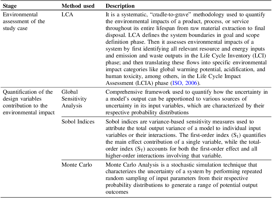
The practical execution of GSA relies on MC simulations, which serve as the computational engine for propagating input uncertainty through the LCA model (Reference Groen, Bokkers, Heijungs and de BoerGroen et al., 2017). This technique requires defining a probability distribution function (PDF) for every input parameter of the Life Cycle Inventory. During each MC iteration, a value is randomly sampled from the PDF of each parameter, defining each time a plausible set of inputs. This set is then used to calculate a full LCA analysis, producing one specific set of output values (Reference Saltelli, Tarantola, Campolongo and RattoSaltelli et al., 2004). The simulation is repeated (hundreds or thousands of times) until a defined confidence threshold is met. The resulting collection of outputs after all the simulations forms a distribution of possible LCA outputs, which are used to calculate the Sobol indexes and identify the most influencing input variables. The concepts used to perform the study are summarized in Table 1.
2.1.3. Sobol indices calculation
Following the MC simulations, the resultant input-output dataset is analyzed using variance-based sensitivity measures with Sobol indices (Reference SobolSobol, 2001). Sobol indices decompose the total variance of the output into fractional contributions of each individual input variable and their combinations. The resulting indices are normalized, with the sum of all terms equaling unity. Input variables with high Sobol index values are confirmed as the most influential (Reference Groen, Bokkers, Heijungs and de BoerGroen et al., 2017; Reference Saltelli, Tarantola, Campolongo and RattoSaltelli et al., 2004).
Summarized methodological framework concepts used

2.2. Case study definition
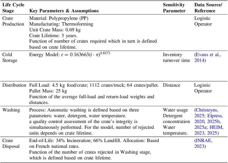
The case study concerns a reuse loop that delivers chilled food from a storage platform to catering sites. The food is transported in plastic crates in a logistic loop comprising the following stages: crate production, usage (food cold storage and distribution), adequacy and assessment for reuse (washing), and crate disposal. For the case study the system manages 1112 plastic crates per day which corresponds to the transport of 5 tons of food. Material, process energy, and transport related exchanges are defined as flows. The model system boundaries are shown in Figure 1. The specific assumptions and parameters used to simulate the system are synthesized in Table 2.
Packaging reuse loop processes and flows scheme

Figure 1 Long description
The flowchart illustrates the processes and flows involved in the reuse loop of packaging crates. The process begins with Crate Production, where plastic undergoes thermoforming to create crates. These crates are then moved to Cold Storage, which requires energy. From Cold Storage, the filled crates proceed to Distribution, which involves transport. After distribution, empty crates are returned and undergo a Washing process using water and detergent. The washed crates are then sent back to Cold Storage, completing the loop. Damaged crates are directed to Crate Disposal, where they are either incinerated or sent to a landfill. The flowchart also indicates support activities such as energy and transport, and waste flows such as wastewater and plastic waste.
Summary of key assumptions and operational parameters for the crate life cycle stages

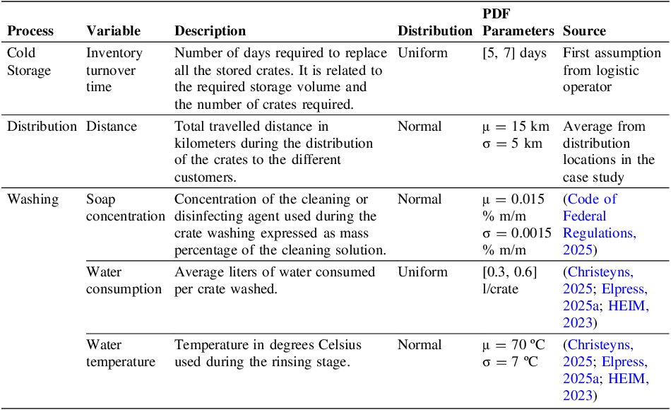
This step defines the ranges and probability distributions of the input variables, which will be sample in the Monte Carlo simulation. Adjusting the underlying assumptions allows the proposed framework to adapt to various operational contexts. For instance, modifications to the spatial configuration of distribution points allow recalibration of the corresponding distance probability distributions. Thus, this scheme establishes a foundational architecture that supports both the parametric variation of the recovery loop and the systematic integration of additional complexities to enhance model fidelity.
2.3. Life Cycle Assessment calculation and Global Sensitivity Analysis setup
The Life Cycle Assessment (LCA) of the reuse loop was performed utilizing the Brightway2 Python library as the computational framework. The Ecoinvent 3.11 database provided the necessary life cycle inventory data for modeling the energy and service flows illustrated in Figure 1. The LCA functional unit (FU) was defined as the one-year operation of a plastic crate reuse loop, processing 1112 crates per day within the Île-de-France region. The chosen LCA methodology was the ReCiPe 2016 V1.03, Midpoint (H) methodology (Reference Huijbregts, Steinmann, Elshout, Stam, Verones, Vieira, Hollander, Zijp and van ZelmHuijbregts et al., 2016).The system analysis was parameterized using the five input variables shown in Table 2. These variables summarize the operational decisions of the involved processes as shown in Table 3.
For Monte Carlo simulation, each input variable was stochastically characterized using specific PDFs. A Normal distribution was assigned to parameters with well-defined mean operational values, while a Uniform distribution was employed for variables where only a feasible range of interval values was available.
System process input variable description

For the LCA process and flow setup, the flows not connected to a process inside Figure 1 (e.g., Energy, Transport) denote background system exchanges, representing inputs of materials, processes, and services. Energy service is modelled as electricity consumption from the French energy mix. The transport service is differentiated: distribution uses a 7.5-ton, Euro 6, refrigerated truck (R134a), while post-washing transport uses a similar but non-refrigerated truck. Life Cycle Inventory (LCI) data for all background services were extracted from the Ecoinvent v3.11 database.
Sampling in the MC simulation for parameter space exploration employed Sobol’s sequence, extended by Reference SaltelliSaltelli (2002), as implemented in the SALib Python library. The number of samples (N) was systematically varied across powers of two, ranging from 2 to 2048, consistent with the recommended practice for this method. The generation of each sample set requires the evaluation of the underlying model, specifically the Life Cycle Assessment (LCA), a total of N(D+2) times, where D represents the number of dimensions (parameters) in the model space. For this study, the dimensionality was fixed at D = 5. The sampling was configured to calculate the first order and total order Sobol indices for sensitivity analysis. To quantify the uncertainty in each estimation a confidence interval of 95% was computed for each resulting Sobol index. The experiments were executed on a computational platform featuring an Intel® Core™ Ultra 7 155H processor and 16 GB DDR5 memory. The computational efficiency of the LCA model was characterized by an average CPU time of 0.98 s per single LCA evaluation.
3. Results and analysis
3.1. Samples number assessment
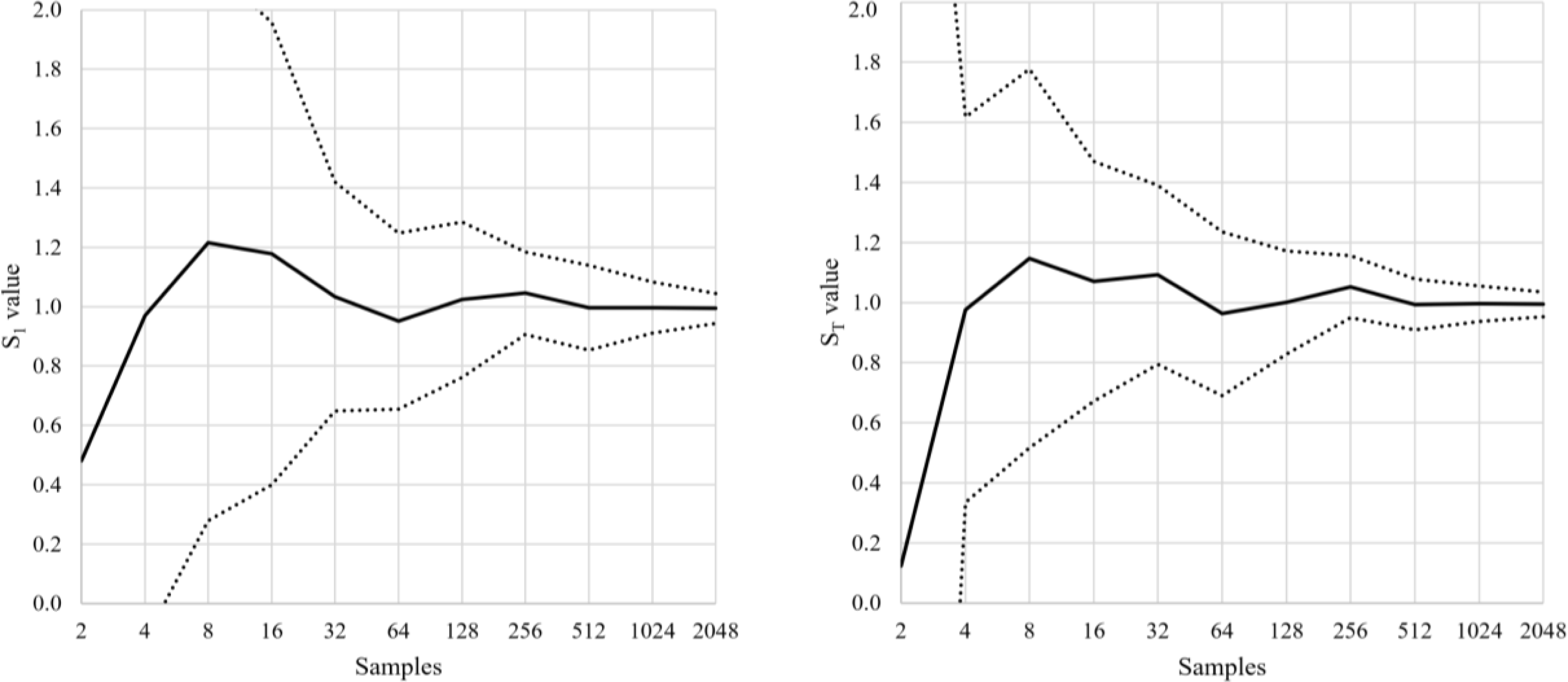
The convergence of the estimated Sobol indices was systematically assessed to ensure statistical robustness. This analysis involved incrementally increasing the number of samples from 2 to 2048 in powers of two. The predefined convergence criterion required that the width of the 95% confidence interval (CI) for each estimated index value must be at most 10% of the index value itself. Achieving this tolerance for statistical stability required a total sample size of 2048 samples for the analyzed loop configuration. Given the computational cost associated with the Sobol index estimation method, this sample size corresponded to a total of 14,336 evaluations of the underlying LCA model.
Figure 2 illustrates the stabilization of the index value of Global Warming Potential (GWP100) and the narrowing of its 95% CI as the sample size increases. Essentially, this convergence trend observed for the GWP100 index is representative of the characteristics found across all 18 environmental indicators assessed within the ReCiPe methodology. Consequently, a sample size of 2048 was adopted for the following analysis of the Sobol indices across all environmental impact categories to guarantee consistent statistical reliability.
First and Total order Sobol index convergence diagram for GWP100 and the distance input parameter. The evolution of the Index value is represented through a continuous line while the 95% confidence interval is represented with a dotted line

3.2. LCA evaluation and Sobol index calculation
A preliminary extreme case analysis was executed to estimate the expected variation in the indicator values. The parameter values selected for this evaluation were determined by their assumed probability distributions. For uniformly distributed parameters, the evaluation included the minimum, mean, and maximum values (lower, average, and upper bounds). For normally distributed parameters, the bounds were set at a distance of two standard deviations (2σ) from the median, effectively covering approximately 95% of the distribution’s probability. These results are detailed in Appendix A.
The preliminary analysis performed on the life cycle impact assessment (LCIA) results demonstrated significant variation across all evaluated environmental categories. The relative variation, resulting from the tested parameter perturbations, spanned a considerable range, extending from a minimum of 29 % for IRP (Ionizing Radiation Potential) to a maximum of 54 % for TETP (Terrestrial Ecotoxicity Potential). These quantitative findings feature the strong dependence of the environmental indicators on the selected modelling parameters.
To assess the contribution of each of the parameters to the environmental indicators, the first order (S1) and total order (ST) Sobol indices were calculated. The results of this analysis are presented in Figure 3, and their corresponding values are shown in Annex B. In each of the sections of the plot both values of Sobol indices are shown for each environmental indicator. This global sensitivity analysis reveals crucial insights into the system’s structure and the dominant drivers of uncertainty across the 18 environmental outputs.
First and Total order Sobol index values per environmental category and parameter. S1 in orange and ST in blue

This global sensitivity analysis identifies the Transport Distance as the main driver for the majority of environmental impact categories, including Global Warming Potential (GWP) and Terrestrial Acidification (TAP), where it accounts for over 90% of the total variance (S1 > 0.9). This indicates that for the reuse loop configuration under analysis, the most effective design strategy to mitigate the system’s general environmental footprint is supply chain optimization and facility localization, rather than process engineering. Conversely, the washing process parameters, Water Consumption and Water Temperature, are specifically decisive for specific categories such as Water Depletion (WCP) and Ionizing Radiation (IRP). Therefore, unless the design is strictly constrained by water scarcity or specific energy grid mixes, efforts to improve washing machine efficiency are secondary to the critical need for reducing logistical expenses.
Finally, the comparison between first order (S1) and total order (ST) indices demonstrates that the reuse loop behaves as a highly linear system with negligible interaction effects. Across almost all categories, the sum of S1 indices approximates 1.0, and ST values closely track their corresponding S1 values (e.g., S1, Distance ≈ ST, Distance for GWP100). This lack of higher-order interactions implies that the environmental impact of logistics and washing are additive rather than multiplicative in the reuse loop configuration under analysis. From a design perspective, this linearity allows for the separate optimization of the logistical network and the washing unit, simplifying the overall optimization problem by eliminating the need to account for complex cross-variable dependencies. This also implies that in systems where the processes are modelled in detail, it is possible that the current representation cannot manage the feasible complex interactions that the detailed model might imply. At a more advanced stage of the research, the analysis will be extended to more accurate representations of the processes, and an attempt will be made to characterize more complex configurations of the reuse cycle (i.e. multi-loop system, closed vs open loop, logistic networks with pooling sites, among others) in order to expand the solution space and capture the effects of additional cycle provisions and process combinations.
4. Conclusions
This study utilized extreme case and Sobol sensitivity analyses to definitively characterize the uncertainty landscape of the LCIA model. The analysis confirmed the suitability of the system for a simple main-effects approach, as the variability in outcomes is mainly governed by the independent, direct effects of the parameters, with negligible interaction contribution (ST ≈ S1). Quantitatively, the Distance parameter is confirmed as the dominant source of variance for most environmental outputs in the case study. In a future step of the research, the influence of other operational variables will be examined in greater depth, by focusing on the effect of transport differentially (e.g. assessing the additional transport generated by reusable packaging and not the total transport that would also exist in the single-use loop systems) to capture the effect of the other variables more accurately.
In the presented case study, since transport distance governed the variance for the majority of environmental impact categories, including Global Warming Potential and Acidification, design efforts must prioritize the optimization of reverse logistics routes to minimize the packaging distribution loop radius. Conversely, investments in washing machine efficiency, specifically targeting water consumption and temperature, should be reserved for scenarios strictly constrained by water scarcity (WCP) or nuclear energy dependence (IRP), as these parameters exert negligible influence on the system’s broader carbon footprint. Furthermore, the demonstrated linearity of the model and the irrelevance of soap concentration validate a decoupled optimization framework, allowing engineers to fix chemical variables and optimize the logistical network independently of the washing unit without the risk of significant cross-subsystem trade-offs. Also, this linearity limits the model conclusions to simplified cases where the considered variables effects have not high order interactions.
Appendix A. LCA extreme values evaluation
Impact
Unit
Low
Mid
Upper
Variation
% Variation
TAP
kg SO2-Eq
48.64
60.83
73.43
24.78
41%
GWP1000
kg CO2-Eq
25181.27
32132.84
39249.39
14068.12
44%
FETP
kg 1,4-DCB-Eq
1184.96
1508.11
1837.33
652.37
43%
METP
kg 1,4-DCB-Eq
1607.54
2048.65
2497.95
890.41
43%
TETP
kg 1,4-DCB-Eq
128911.11
176178.76
224046.55
95135.45
54%
FFP
kg oil-Eq
7963.09
10079.40
12238.63
4275.54
42%
FEP
kg P-Eq
4.61
5.76
6.95
2.34
41%
MEP
kg N-Eq
4.16
5.12
6.11
1.96
38%
HTPc
kg 1,4-DCB-Eq
4678.46
6034.34
7422.40
2743.94
45%
HTPnc
kg 1,4-DCB-Eq
30986.79
38188.37
45622.77
14635.99
38%
IRP
kg Co-60-Eq
57317.80
66576.04
76823.22
19505.42
29%
LOP
m2*a crop-Eq
574.85
728.60
887.77
312.91
43%
SOP
kg Cu-Eq
629.52
819.15
1012.71
383.19
47%
ODPinfinite
kg CFC-11-Eq
0.01
0.02
0.02
0.01
41%
PMFP
kg PM2.5-Eq
21.13
26.56
32.17
11.04
42%
HOFP
kg NOx-Eq
43.25
54.27
65.63
22.38
41%
EOFP
kg NOx-Eq
47.07
59.18
71.63
24.56
42%
WCP
m3
374.97
440.42
511.66
136.69
31%
Appendix B. Sensitivity analysis Sobol index values




 Open access

