


1. Introduction
A network is a graph structure that depicts intricate systems as nodes and edges, where nodes represent objects and edges express their relationships. Edge weights can quantify the strength of these relationship, with higher edge weights indicating a stronger connection. Complex real-world systems, such as urban transportation networks, airline networks, computer communication networks, and social networks, are characterised by their members’ relationships. It is a daunting, if not impossible, task to understand the structure of a network through direct (visual) observation, especially when the numbers of nodes and edges are large. It is important, therefore, to be able to accurately and efficiently detect relevant characteristics of networks.
A typical characteristic of networks is their community structure and its detection involves partitioning the set of nodes into different communities (or clusters). Intuitively a network has a community structure if the node set can be partitioned in such a way that nodes within each resulting cluster are more likely to be connected to each other than to nodes in other clusters. Different mathematically precise measures have been proposed in the literature to capture this intuitive notion. In this paper, we will focus on modularity [Reference Newman56, Reference Newman and Girvan57], which, for a given partitioning of the node set, quantifies the difference between the actual connectivity structure within each cluster and the expected connectivity structure based on a random null model. We give the precise definition in Section 2.3.
Community detection is of great theoretical and practical value for understanding the topology and predicting the behaviour of real-world networks and has been widely used in many fields, such as protein function prediction [Reference Perlasca, Frasca, Ba, Gliozzo, Notaro, Pennacchioni, Valentini, Mesiti and Cherifi60] and criminology [Reference Karataş and Şahin38]. The formulation of modularity suggests that its maximisation over all possible partitions of the node set allows one to detect communities in a given network. Modularity optimisation, however, is an NP-hard problem [Reference Brandes, Delling, Gaertler, Gorke, Hoefer, Nikoloski and Wagner9]; thus, numerous algorithms have been developed to approximately optimise modularity, including extremal optimisation [Reference Duch and Arenas21], greedy algorithms such as the Clauset–Newman–Moore algorithm (CNM) [Reference Clauset, Newman and Moore19], the Louvain algorithm [Reference Blondel, Guillaume, Lambiotte and Lefebvre6], the Leiden algorithm [Reference Traag, Waltman and van Eck71], simulated annealing [Reference Guimerà, Sales-Pardo and Amaral28], spectral methods [Reference Girvan and Newman26, Reference Newman56], and a proximal gradient method [Reference Sun and Chang67].
Hu et al. [Reference Hu, Laurent, Porter and Bertozzi33] presented a total variation (TV)-based approach for optimising network modularity using a Merriman–Bence–Osher (MBO) type scheme. The MBO scheme, originally formulated as an efficient way to approximate flows by mean curvature in Merriman et al. [Reference Merriman, Bence and Osher50, Reference Merriman, Bence and Osher51] and co-opted as a fast method for approximately solving graph classification problems by Merkurjev et al. [Reference Merkurjev, Kostić and Bertozzi49], is an iterative algorithm that combines short-time (linear) dynamics with thresholding. By changing the specifics of the dynamics, different MBO-type schemes can be constructed and Boyd et al. [Reference Boyd, Bae, Tai and Bertozzi7] suggested an alternative MBO scheme for modularity optimisation which, unlike the scheme of [Reference Hu, Laurent, Porter and Bertozzi33], is based on an underlying convex approximation of modularity.
One significant advantage of MBO-type schemes is their flexibility to incorporate extra data or constraints into the scheme, for example, a fidelity-forcing term based on training data in the linear-dynamics step as in Budd et al. [Reference Budd, van Gennip and Latz12] or a mass-conservation constraint in the thresholding step as in Budd and van Gennip [Reference Budd and Van Gennip11]. The underlying models that form the basis of MBO schemes also make rigorous analysis possible, often help interpretability of the method, and amplify the impact of even small numbers of training data. Moreover, the general form of MBO schemes – linear dynamics alternated with non-linear thresholding steps – makes them amenable to incorporation into artificial neural networks, as in Liu et al. [Reference Liu, Liu, Chan and Tai45]. In the current paper, we focus on MBO schemes that only use the available weighted graph structure and no additional training data or mass constraints.
1.1. Contributions
Our main contribution is the development and rigorous analysis of a new MBO-type method for modularity optimisation, which we name the modularity MBO (MMBO) method. From a theoretical point of view, our method distinguishes itself from the prior MBO-type methods in [Reference Hu, Laurent, Porter and Bertozzi33] and [Reference Boyd, Bae, Tai and Bertozzi7] in that the influence of the chosen null model on the algorithm is explicit. This is due to the fact that we reformulate the modularity objective function in terms of a total variation functional on the ‘observed’ network whose communities we aim to detect and a signless total variation functional on the expected network under the null model. This signless total variation was a key ingredient in the maximum cut algorithm in [Reference Keetch and van Gennip39]. Modularity optimisation can thus be interpreted as balancing a minimum cut problem on the observed network with a maximum cut problem on the expected network under the null model. This also allows for the easy adaptation of the new method to the use of different null models in the modularity function.Footnote 1
We perform an in-depth theoretical study of the (various variants of the) linear operator $L_{\textrm{mix}}$
that appears in the linear-dynamics step of our MMBO algorithm, guaranteeing that the algorithm is well defined. Besides allowing six variants of the linear operator, we also formulate two different variants of the MMBO algorithm that differ in the method they use to numerically compute the linear-dynamics step. Finally, we test our method on networks formed by the MNIST handwritten digits data set [Reference LeCun, Cortes and Christopher43], a stochastic block model (SBM) [Reference Holland, Laskey and Leinhardt32] and a ‘two cows’ image [Reference Bertozzi and Flenner4]. We compare our method with the modularity optimisation methods of Clauset et al. [Reference Clauset, Newman and Moore19] (CNM), Blondel et al. [Reference Blondel, Guillaume, Lambiotte and Lefebvre6] (Louvain), Traag et al. [Reference Traag, Waltman and van Eck71] (Leiden), Hu et al. [Reference Hu, Laurent, Porter and Bertozzi33] and Boyd et al. [Reference Boyd, Bae, Tai and Bertozzi7], as well as with spectral clustering [Reference Jianbo Shi and Malik37], which was developed for graph clustering, but not specifically for modularity optimisation. Because of our focus on methods that do not use any training data, we do not compare with artificial-neural-network-based methods.
$L_{\textrm{mix}}$
that appears in the linear-dynamics step of our MMBO algorithm, guaranteeing that the algorithm is well defined. Besides allowing six variants of the linear operator, we also formulate two different variants of the MMBO algorithm that differ in the method they use to numerically compute the linear-dynamics step. Finally, we test our method on networks formed by the MNIST handwritten digits data set [Reference LeCun, Cortes and Christopher43], a stochastic block model (SBM) [Reference Holland, Laskey and Leinhardt32] and a ‘two cows’ image [Reference Bertozzi and Flenner4]. We compare our method with the modularity optimisation methods of Clauset et al. [Reference Clauset, Newman and Moore19] (CNM), Blondel et al. [Reference Blondel, Guillaume, Lambiotte and Lefebvre6] (Louvain), Traag et al. [Reference Traag, Waltman and van Eck71] (Leiden), Hu et al. [Reference Hu, Laurent, Porter and Bertozzi33] and Boyd et al. [Reference Boyd, Bae, Tai and Bertozzi7], as well as with spectral clustering [Reference Jianbo Shi and Malik37], which was developed for graph clustering, but not specifically for modularity optimisation. Because of our focus on methods that do not use any training data, we do not compare with artificial-neural-network-based methods.
The contributions of this paper are as follows:
-
• a reformulation of modularity in terms of (signless) total variations functions (Section 3);
-
• the development of a new MBO-type method for modularity optimisation, which does not require a specific form of the null model (Section 5);
-
• a rigorous analysis of various aspects of the method, such as the matrices involved (Sections 3–5);
-
• the identification of different operators for the linear thresholding step following a careful consideration of the inner products underlying the method (Sections 4–5);
-
• comparative computational tests, which not only show the performance of the new method in relation to existing methods measured according to the obtained modularity scores and various extrinsic clustering quality scores but also serve as a replication of results for the existing methods (Section 7);
-
• an empirical investigation of the dependence of the methods by Hu et al., by Boyd et al., and the new methods on the number of eigenvectors of the linear operator that are used and the number of iterations of the algorithm (Section 7).
1.2. Paper outline
The remainder of the paper is organised as follows. In Section 2, we introduce the mathematical preliminaries that we need; in particular in Section 2.3, we (re)acquaint the reader with the modularity function.
The reformulation of modularity in terms of a total variation and signless total variation function is key to our method. We present this reformulation in Section 3, both for the case of two communities and multiple (i.e., more than two) communities.
On our way to formulating an MBO-type scheme for modularity optimisation, we require a relaxation of the original problem. This we achieve via the Ginzburg–Landau (GL) diffuse-interface techniques that we describe in Section 4.
After this, the stage is ready for the introduction of our MMBO schemes for binary community detection and multi-community detection in Section 5. The details of the numerical implementations of these schemes are discussed in Section 6, such as the Nyström extension with QR decomposition [Reference Bertozzi and Flenner4, Reference Budd, van Gennip and Latz12, Reference Fowlkes, Belongie, Fan and Malik23, Reference Nyström58] in Section 6.4, which is employed to efficiently compute the leading eigenvalues and eigenvectors of our operators.
In Section 7, we evaluate the performance of our method on synthetic and real-world networks, not only in terms of modularity optimisation and run time but also according to various performance metrics (described in Section 7.1.3) that compare the algorithms’ output with ground truth community structures that are available for the data sets we use for our tests.
We close the main part of the paper in Section 8 with some conclusions and suggestions for future research.
In Appendix A, we establish some properties of two multi-well potentials. The other appendices provide theoretical results regarding the spectra of the operators we use in the linear-dynamics step of our MMBO scheme. Appendices B and C present deferred proofs for lemmas from Sections 5 and 6, respectively, while Appendix D investigates the consequences that Weyl’s inequality and a rank-one matrix update theorem have for our operators.
Notation. Table 1 contains an overview of notation that is frequently used in this paper.
Summary of frequently used symbols

2. Mathematical preliminaries
In this section, we introduce basic terminology and derive a new formulation of modularity maximisation in terms of the minimisation of a combination of graph total variation and graph signless total variation.
2.1. Graphical framework
In this paper, we consider connected, edge-weighted, undirected graphs $G = (V, E, \omega )$
with a node set
$G = (V, E, \omega )$
with a node set $V = \{1, \ldots, |V|\}$
, an edge set
$V = \{1, \ldots, |V|\}$
, an edge set $E=\{ (i,j) \}^{|V|}_{i,j=1}$
, and edge weight
$E=\{ (i,j) \}^{|V|}_{i,j=1}$
, and edge weight $\omega _{ij}$
between node
$\omega _{ij}$
between node $i$
and node
$i$
and node $j$
. The (weighted) adjacency matrix
$j$
. The (weighted) adjacency matrix $W=( \omega _{ij})^{|V|}_{i,j=1}$
is a symmetric matrix whose entries
$W=( \omega _{ij})^{|V|}_{i,j=1}$
is a symmetric matrix whose entries $\omega _{ij}$
are zero if
$\omega _{ij}$
are zero if $i=j$
or
$i=j$
or $(i,j) \notin E$
, and positiveFootnote
2
otherwise. Consequently, we can consider a given adjacency matrix
$(i,j) \notin E$
, and positiveFootnote
2
otherwise. Consequently, we can consider a given adjacency matrix $W$
(with non-negative entries and zeros on the diagonal) as defining the edge structure of the graph. Graphs with non-negative edge weights are known as unsigned graphs. We consider unweighted graphs as special cases of weighted graphs for which, for all
$W$
(with non-negative entries and zeros on the diagonal) as defining the edge structure of the graph. Graphs with non-negative edge weights are known as unsigned graphs. We consider unweighted graphs as special cases of weighted graphs for which, for all $i,j\in V$
,
$i,j\in V$
, $\omega _{ij}\in \{0,1\}$
.
$\omega _{ij}\in \{0,1\}$
.
We will reserve the notation $W$
for the adjacency matrix of the connected graph whose nodes we wish to cluster. Along the way we also encounter graphs defined by other adjacency matrices; therefore in our definitions of adjacency-matrix-dependent quantities, we will use the (dummy) symmetric matrix
$W$
for the adjacency matrix of the connected graph whose nodes we wish to cluster. Along the way we also encounter graphs defined by other adjacency matrices; therefore in our definitions of adjacency-matrix-dependent quantities, we will use the (dummy) symmetric matrix $C\in [0,\infty )^{|V|\times |V|}$
with entries
$C\in [0,\infty )^{|V|\times |V|}$
with entries $c_{ij}$
. We note that we do not require the diagonal entries
$c_{ij}$
. We note that we do not require the diagonal entries $c_{ii}$
to be zero, as is sometimes required in other sources (i.e., we allow the graph defined by
$c_{ii}$
to be zero, as is sometimes required in other sources (i.e., we allow the graph defined by $C$
to have self-loops).
$C$
to have self-loops).
We denote the set of neighbours of node $i\in V$
with respect to the adjacency matrix
$i\in V$
with respect to the adjacency matrix $C$
by:
$C$
by:
 \begin{equation*} \mathcal {N}_C(i) \;:\!=\; \{j\in V \;:\; c_{ij} \gt 0\}. \end{equation*}
The (weighted) degree of node $i$
with respect to the adjacency matrix
$i$
with respect to the adjacency matrix $C$
is
$C$
is
 \begin{equation} (d_C)_i\;:\!=\; \sum _{j\in V} c_{ij}. \end{equation}
The diagonal degree matrix $D_C$
of
$D_C$
of $C$
has entries
$C$
has entries $\left (D_C \right )_{ii}=(d_C)_i$
. The maximum and minimum node degrees with respect to
$\left (D_C \right )_{ii}=(d_C)_i$
. The maximum and minimum node degrees with respect to $C$
are
$C$
are
 \begin{equation*} d_{C,\textrm {max}} \;:\!=\; \max _{i\in V} (d_C)_i \quad \text {and} \quad d_{C,\textrm {min}} \;:\!=\; \min _{i\in V} (d_C)_i, \end{equation*}
respectively. The volume (i.e., total edge weight) of a subset $S\subset V$
with respect to
$S\subset V$
with respect to $C$
is defined as:
$C$
is defined as:
 \begin{equation*} \textrm {vol}_C(S)\;:\!=\;\sum _{i\in S} (d_C)_i = \sum _{i \in S, j \in V} c_{ij}. \end{equation*}
In particular, $\textrm{vol}_C(V)$
is also called the volume of the graph with adjacency matrix
$\textrm{vol}_C(V)$
is also called the volume of the graph with adjacency matrix $C$
.
$C$
.
We define the set of real-valued node functions:
 \begin{equation*} \mathcal {V} \;:\!=\; \left \{u\;:\; V \to \mathbb {R}\right \}. \end{equation*}
Since a function $u \in \mathcal{V}$
is fully determined by its values
$u \in \mathcal{V}$
is fully determined by its values $u_1, \ldots, u_{|V|}$
at the (finitely many) nodes, we may equivalently interpret
$u_1, \ldots, u_{|V|}$
at the (finitely many) nodes, we may equivalently interpret $u$
as a column vector
$u$
as a column vector $(u_1, \ldots, u_{|V|})^T \in \mathbb{R}^{|V|}$
. We will freely make use of both the interpretation as function and as vector and do not distinguish between the two in our notation. As a consequence, we can represent linear operators that act on functions
$(u_1, \ldots, u_{|V|})^T \in \mathbb{R}^{|V|}$
. We will freely make use of both the interpretation as function and as vector and do not distinguish between the two in our notation. As a consequence, we can represent linear operators that act on functions $u\;:\; V \to \mathbb{R}$
by
$u\;:\; V \to \mathbb{R}$
by $|V|$
-by-
$|V|$
-by- $|V|$
real matrices. Also in this context, we will not distinguish between the operator and matrix interpretations in our notation.
$|V|$
real matrices. Also in this context, we will not distinguish between the operator and matrix interpretations in our notation.
The standard (Euclidean) inner product $\langle \cdot, \cdot \rangle$
on
$\langle \cdot, \cdot \rangle$
on $\mathbb{R}^{|V|}$
is defined as
$\mathbb{R}^{|V|}$
is defined as $\langle u, v \rangle \;:\!=\;u^T v$
. The norms
$\langle u, v \rangle \;:\!=\;u^T v$
. The norms $||\cdot ||_1$
and
$||\cdot ||_1$
and $||\cdot ||_2$
are the taxicab norm (i.e.,
$||\cdot ||_2$
are the taxicab norm (i.e., $1$
-norm) and the Euclidean norm (i.e.,
$1$
-norm) and the Euclidean norm (i.e., $2$
-norm), respectively; that is, for vectors
$2$
-norm), respectively; that is, for vectors $w\in \mathbb{R}^n$
,Footnote
3
$w\in \mathbb{R}^n$
,Footnote
3
 \begin{equation*} \|w\|_1 \;:\!=\; \sum _{i=1}^n |w_n| \quad \text {and} \quad \|w\|_2 \;:\!=\; \left (\sum _{i=1}^n w_n^2\right )^{\frac {1}{2}}. \end{equation*}
If $C$
does not contain a row with only zeros, that is, if all row sums
$C$
does not contain a row with only zeros, that is, if all row sums $(d_C)_i$
are positive, we define the
$(d_C)_i$
are positive, we define the $C$
-degree-weighted inner product to be
$C$
-degree-weighted inner product to be
 \begin{equation} \langle u, v \rangle _C \;:\!=\; \sum _{i\in V} u_i v_i (d_C)_i. \end{equation}
For future reference we note that, if $C$
and
$C$
and $\tilde C$
are two adjacency matrices with positive row sums, then
$\tilde C$
are two adjacency matrices with positive row sums, then
 \begin{equation} \langle u, v \rangle _C = \langle D_{\tilde C}^{-1} D_C u, v \rangle _{\tilde C}. \end{equation}
Given an adjacency matrix $C$
, and a function
$C$
, and a function $u\;:\; V \rightarrow \mathbb{R}$
, we define the graph total variation (
$u\;:\; V \rightarrow \mathbb{R}$
, we define the graph total variation ( $TV_C$
) and graph signless total variation (
$TV_C$
) and graph signless total variation ( $TV_C^+$
) as:
$TV_C^+$
) as:
 \begin{equation*} TV_C (u)\;:\!=\; \frac {1}{2} \sum _{i,j \in V} c_{ij} |u_i -u_j| \quad \text {and} \quad TV_C^+ (u)\;:\!=\; \frac {1}{2} \sum _{i,j \in V} c_{ij} |u_i + u_j|. \end{equation*}
A vector-valued node function $u=(u^{(1)}, \ldots, u^{(K)})\;:\;V \rightarrow \mathbb{R}^{K}$
, where
$u=(u^{(1)}, \ldots, u^{(K)})\;:\;V \rightarrow \mathbb{R}^{K}$
, where $u^{(l)}$
is the
$u^{(l)}$
is the $l^{\text{th}}$
component of
$l^{\text{th}}$
component of $u$
, can be interpreted as a matrix
$u$
, can be interpreted as a matrix $U\in \mathbb{R}^{|V|\times K}$
, with elements
$U\in \mathbb{R}^{|V|\times K}$
, with elements $U_{il} \;:\!=\; u_i^{(l)}$
. We write
$U_{il} \;:\!=\; u_i^{(l)}$
. We write $U_{*l}$
for the
$U_{*l}$
for the $l^{\text{th}}$
column of
$l^{\text{th}}$
column of $U$
; thus, the column vector
$U$
; thus, the column vector $U_{*l}$
is the vector representation of the function
$U_{*l}$
is the vector representation of the function $u^{(l)}\;:\; V \to \mathbb{R}$
. We write
$u^{(l)}\;:\; V \to \mathbb{R}$
. We write $U_{j*}$
for
$U_{j*}$
for $U$
’s
$U$
’s $j^{\text{th}}$
row. As with the vector interpretation of real-valued node functions above, we freely use the interpretation as function or as matrix, as suits our purpose.
$j^{\text{th}}$
row. As with the vector interpretation of real-valued node functions above, we freely use the interpretation as function or as matrix, as suits our purpose.
For vector-valued node functions $u$
, we generalise the definition of graph total variation and graph signless total variation to
$u$
, we generalise the definition of graph total variation and graph signless total variation to
 \begin{align*} \mathcal{TV}_C (u)\;:\!=\;\sum _{l=1}^{K} TV_C (u^{(l)}) = \frac{1}{2} \sum _{l=1}^{K} \sum _{i,j \in V} c_{ij} \left |u_i^{(l)} - u_j^{(l)}\right | = \frac{1}{2} \sum _{l=1}^{K} \sum _{i,j \in V} c_{ij} \left |U_{il} - U_{jl}\right |,\\[5pt] \mathcal{TV}_C^+ (u)\;:\!=\;\sum _{l=1}^{K} TV_C^+ (u^{(l)}) = \frac{1}{2} \sum _{l=1}^{K} \sum _{i,j \in V} c_{ij} \left |u_i^{(l)} + u_j^{(l)}\right | = \frac{1}{2} \sum _{l=1}^{K} \sum _{i,j \in V} c_{ij} \left |U_{il} + U_{jl}\right |. \end{align*}
For a matrix $U\in \mathbb{R}^{n\times p}$
with entries
$U\in \mathbb{R}^{n\times p}$
with entries $U_{ij}$
, its
$U_{ij}$
, its $C$
-Frobenius norm (with
$C$
-Frobenius norm (with $C\in \mathbb{R}^{n\times n}$
symmetric positive definiteFootnote
4
) is given by:
$C\in \mathbb{R}^{n\times n}$
symmetric positive definiteFootnote
4
) is given by:
 \begin{equation*} \|U\|_{\textrm {Fr},C} \;:\!=\; \sqrt {\textrm {tr}(U^TCU)} = \sqrt {\sum _{j=1}^p \sum _{k, l=1}^n C_{kl} U_{kj} U_{lj}}, \end{equation*}
where $\textrm{tr}$
denotes the trace of a square matrix. If
$\textrm{tr}$
denotes the trace of a square matrix. If $C$
is the identity matrix
$C$
is the identity matrix $I$
, this reduces to the standard Frobenius norm
$I$
, this reduces to the standard Frobenius norm $\|U\|_{\textrm{Fr}} \;:\!=\; \|U\|_{_{\textrm{Fr},I}}$
. Because the standard Frobenius norm is submultiplicative, that is, for all matrices
$\|U\|_{\textrm{Fr}} \;:\!=\; \|U\|_{_{\textrm{Fr},I}}$
. Because the standard Frobenius norm is submultiplicative, that is, for all matrices $U_1 \in \mathbb{R}^{n\times p}$
and
$U_1 \in \mathbb{R}^{n\times p}$
and $U_2 \in \mathbb{R}^{p\times q}$
,
$U_2 \in \mathbb{R}^{p\times q}$
, $\|U_1U_2\|_{\textrm{Fr}} \leq \|U_1\|_{\textrm{Fr}} \|U_2\|_{\textrm{Fr}}$
, the
$\|U_1U_2\|_{\textrm{Fr}} \leq \|U_1\|_{\textrm{Fr}} \|U_2\|_{\textrm{Fr}}$
, the $C$
-Frobenius norm satisfies the following property:
$C$
-Frobenius norm satisfies the following property:
 \begin{equation} \|U_1 U_2\|_{\textrm{Fr},C} = \|C^{\frac 12} U_1 U_2\|_{\textrm{Fr}} \leq \|C^{\frac 12} U_1\|_{\textrm{Fr}} \|U_2\|_{\textrm{Fr}} = \|U_1\|_{\textrm{Fr},C} \|U_2\|_{\textrm{Fr}}. \end{equation}
The infinity operator norm of the matrix $U$
is given by:
$U$
is given by:
 \begin{equation*} \|U\|_\infty \;:\!=\; \max _{i\in \{1, \ldots, n\}} \sum _{j=1}^p |U_{ij}|. \end{equation*}
Given $K\in \mathbb{N}$
, let
$K\in \mathbb{N}$
, let $\mathcal{A}=\{A_l\}_{l=1}^{K}$
be a multisetFootnote
5
of pairwise disjoint subsets of
$\mathcal{A}=\{A_l\}_{l=1}^{K}$
be a multisetFootnote
5
of pairwise disjoint subsets of $V$
that partition the node set
$V$
that partition the node set $V$
, that is,
$V$
, that is, $V=\bigcup _{l=1}^{K} A_l$
and
$V=\bigcup _{l=1}^{K} A_l$
and $A_{l_1} \cap A_{l_2} = \emptyset$
if
$A_{l_1} \cap A_{l_2} = \emptyset$
if $l_1 \neq l_2$
. Note that
$l_1 \neq l_2$
. Note that $A_l$
could be empty, so the number of non-empty sets in
$A_l$
could be empty, so the number of non-empty sets in $\mathcal{A}$
is at most
$\mathcal{A}$
is at most $K$
. We call two partitions (with possibly different numbers of elements) equivalent, if every element of their symmetric difference is
$K$
. We call two partitions (with possibly different numbers of elements) equivalent, if every element of their symmetric difference is $\emptyset$
. The canonical representative of an equivalence class of partitions is the unique partition in the equivalence class that does not contain any copy of
$\emptyset$
. The canonical representative of an equivalence class of partitions is the unique partition in the equivalence class that does not contain any copy of $\emptyset$
. Each canonical representative
$\emptyset$
. Each canonical representative $\mathcal{A}$
is in bijective correspondence to a node assignment
$\mathcal{A}$
is in bijective correspondence to a node assignment $c\;:\; V \to \{1, \ldots, |\mathcal{A}|\}$
: given a canonical representative
$c\;:\; V \to \{1, \ldots, |\mathcal{A}|\}$
: given a canonical representative $\mathcal{A}=\{A_l\}_{l=1}^{K}$
, define
$\mathcal{A}=\{A_l\}_{l=1}^{K}$
, define $c_j=l$
if and only if
$c_j=l$
if and only if $j\in A_l$
; conversely, given a node assignment
$j\in A_l$
; conversely, given a node assignment $c\;:\; V \to \{1, \ldots, K\}$
, define
$c\;:\; V \to \{1, \ldots, K\}$
, define $A_l=\{j \in V:c_j=l\}$
for
$A_l=\{j \in V:c_j=l\}$
for $l\in \{1, \ldots, K\}$
.
$l\in \{1, \ldots, K\}$
.
We will refer to the sets $A_l$
in a partition as the communities defined by that partition. Also the terms ‘clusters’ or ‘classes’ may be used. We use an indicator function
$A_l$
in a partition as the communities defined by that partition. Also the terms ‘clusters’ or ‘classes’ may be used. We use an indicator function $\delta$
with
$\delta$
with $\delta (c_i,c_j)=1$
if nodes
$\delta (c_i,c_j)=1$
if nodes $i$
and
$i$
and $j$
are in the same community and
$j$
are in the same community and $\delta (c_i,c_j)=0$
otherwise.
$\delta (c_i,c_j)=0$
otherwise.
2.2. Laplacians for unsigned graphs
In this section, we define graph Laplacians for unsigned graphs determined by an adjacency matrix $C$
.
$C$
.
For a graph with weighted adjacency matrix $C$
, we define the graph Laplacian matrix
$C$
, we define the graph Laplacian matrix $L_C$
as [Reference Chung16]:
$L_C$
as [Reference Chung16]:
 \begin{align*} (L_C)_{ij} \;:\!=\; \begin{cases} (d_C)_i - c_{ii}, &\text{if } i=j, \\[5pt] -c_{ij}, &\text{otherwise}. \end{cases} \end{align*}
We include the dependence on $C$
explicitly in the notation, since we require graph Laplacians for various different graphs.
$C$
explicitly in the notation, since we require graph Laplacians for various different graphs.
The Laplacian matrix can be written as:
 \begin{equation*} L_C = D_C - C. \end{equation*}
If $D_C$
is invertible, the random walk graph Laplacian matrix
$D_C$
is invertible, the random walk graph Laplacian matrix $L_{C_{\textrm{rw}}}$
and the symmetrically normalised graph Laplacian matrix
$L_{C_{\textrm{rw}}}$
and the symmetrically normalised graph Laplacian matrix $L_{C_{\textrm{sym}}}$
are given by:
$L_{C_{\textrm{sym}}}$
are given by:
 \begin{align*} L_{C_{\textrm{rw}}} &\;:\!=\; D_C^{-1} L_C = I - D_C^{-1} C,\\[5pt] L_{C_{\textrm{sym}}} &\;:\!=\;D_C^{-\frac{1}{2}} L_C D_C^{-\frac{1}{2}}= I-D_C^{-\frac{1}{2}} C D_C^{-\frac{1}{2}}, \end{align*}
respectively. It is well known that the random walk graph Laplacian and symmetrically normalised graph Laplacian have the same eigenvalues [Reference von Luxburg74].
In the special case that $C=W$
, we recall that
$C=W$
, we recall that $G=(V,E, \omega )$
is connected, and in particular there is no isolated node. Thus, for all
$G=(V,E, \omega )$
is connected, and in particular there is no isolated node. Thus, for all $i\in V$
,
$i\in V$
, $(d_W)_i\gt 0$
and hence the matrix
$(d_W)_i\gt 0$
and hence the matrix $D_W$
is invertible.
$D_W$
is invertible.
Let $u\in \mathbb{R}^{|V|}$
. We compute, for
$u\in \mathbb{R}^{|V|}$
. We compute, for $i\in V$
,
$i\in V$
,
 \begin{equation} (L_C u)_i = \sum _{j\in V} c_{ij} \left ( u_i - u_j \right ) \quad \text{and} \quad \left ( L_{C_{\textrm{rw}}} u\right )_i = \frac{1}{(d_C)_i} \sum _{j\in V} c_{ij} (u_i -u_j), \end{equation}
where we require $(d_C)_i\gt 0$
for the second computation. We note that any self-loops (i.e.,
$(d_C)_i\gt 0$
for the second computation. We note that any self-loops (i.e., $c_{ii}\gt 0$
) do not contribute to the images of the Laplacian
$c_{ii}\gt 0$
) do not contribute to the images of the Laplacian $L_C$
but will contribute to the degree normalisation in
$L_C$
but will contribute to the degree normalisation in $L_{C_{\textrm{rw}}}$
.
$L_{C_{\textrm{rw}}}$
.
Lemma 2.1.
Let $C\in [0,\infty )^{|V|\times |V|}$
be a symmetric matrix. For parts
(b)
and
(c)
below, additionally assume that
$C\in [0,\infty )^{|V|\times |V|}$
be a symmetric matrix. For parts
(b)
and
(c)
below, additionally assume that $D_C$
is invertible.
$D_C$
is invertible.
-
(a) The graph Laplacian (matrix) $L_C$
is self-adjoint with respect to the Euclidean inner product, that is, for all
$u, v\in \mathcal{V}$
,It is also positive semidefinite with respect to the Euclidean inner product Footnote 6 , that is, for all
\begin{equation*} \langle L_C u, v\rangle = \langle u, L_C v\rangle . \end{equation*}
$u\in \mathcal{V}$
,
\begin{equation*} \langle L_C u, u \rangle \geq 0. \end{equation*}
$L_C$
is self-adjoint with respect to the Euclidean inner product, that is, for all
$u, v\in \mathcal{V}$
,It is also positive semidefinite with respect to the Euclidean inner product Footnote 6 , that is, for all
\begin{equation*} \langle L_C u, v\rangle = \langle u, L_C v\rangle . \end{equation*}
$u\in \mathcal{V}$
,
\begin{equation*} \langle L_C u, u \rangle \geq 0. \end{equation*}
-
(b) The symmetrically normalised graph Laplacian (matrix)
$L_{C_{\textrm{sym}}}$
is self-adjoint and positive semidefinite with respect to the Euclidean inner product, that is, for all
$u,v\in \mathcal{V}$
,respectively.
\begin{equation*} \langle L_{C_{\textrm {sym}}} u, v\rangle = \langle u, L_{C_{\textrm {sym}}} v\rangle \quad \text {and} \quad \langle L_{C_{\textrm {sym}}} u, u \rangle \geq 0, \end{equation*}
-
(c) The random walk graph Laplacian (matrix)
$L_{C_{\textrm{rw}}}$
is self-adjoint and positive semidefinite with respect to the
$C$
-degree-weighted inner product, that is, for all
$u,v\in \mathcal{V}$
,respectively.
\begin{equation*} \langle L_{C_{\textrm {rw}}} u, v\rangle _C = \langle u, L_{C_{\textrm {rw}}} v\rangle _C \quad \text {and} \quad \langle L_{C_{\textrm {rw}}} u, u \rangle _C \geq 0, \end{equation*}


Proof. Let $u,v\in \mathcal{V}$
.
$u,v\in \mathcal{V}$
.
It follows from the symmetry of $C$
and (5) that
$C$
and (5) that $L_C$
is self-adjoint with respect to the Euclidean inner product:
$L_C$
is self-adjoint with respect to the Euclidean inner product:
 \begin{equation*} \langle u, L_C v\rangle = \sum _{i,j\in V} c_{ij} u_i (v_i-v_j) = \sum _{i,j\in V} \left (c_{ij} u_i v_i - c_{ji} u_j v_i \right ) = \sum _{i,j\in V} c_{ij} v_i (u_i-u_j) = \langle L_C u, v\rangle . \end{equation*}
Interchanging the indices $i$
and
$i$
and $j$
in this calculation shows in a straightforward way that
$j$
in this calculation shows in a straightforward way that $L_C$
is positive semidefinite:
$L_C$
is positive semidefinite:
 \begin{equation} \langle L_C u, u \rangle =\frac 12 \big (\langle L_C u, u \rangle + \langle u, L_C u\rangle \big ) =\frac{1}{2} \sum _{i,j\in V} c_{ij} (u_i-u_j)^2 \geq 0. \end{equation}
Similarly, the symmetrically normalised graph Laplacian $L_{C_{\textrm{sym}}}$
is self-adjoint with respect to the Euclidean inner product, since
$L_{C_{\textrm{sym}}}$
is self-adjoint with respect to the Euclidean inner product, since
 \begin{equation*} \langle u, L_{C_{\textrm {sym}}} v \rangle = \langle D_C^{-\frac 12} u, L_C D_C^{-\frac 12} v \rangle = \langle L_C D_C^{-\frac 12} u, D_C^{-\frac 12} v \rangle = \langle L_{C_{\textrm {sym}}} u, v \rangle, \end{equation*}
and it is positive semidefinite with respect to the same inner product:
 \begin{align} \langle L_{C_{\textrm{sym}}} u, u \rangle = \frac 12 \big (\langle L_{W_{\textrm{sym}}} u, u \rangle + \langle u, L_{W_{\textrm{sym}}} u\rangle \big ) =\frac{1}{2} \sum _{i,j\in V} c_{ij} \left (\frac{u_i}{\sqrt{(d_C)_i}} - \frac{u_j}{\sqrt{(d_C)_j}} \right )^2 \geq 0. \end{align}
We recall that, for all $i\in V$
,
$i\in V$
, $(d_C)_i\gt 0$
, because the diagonal matrix
$(d_C)_i\gt 0$
, because the diagonal matrix $D_C$
is invertible.
$D_C$
is invertible.
Finally, using (5) we compute
 \begin{equation*} \langle u, L_{C_{\textrm {rw}}} v\rangle _C = \langle u, D_C L_{C_{\textrm {rw}}} v \rangle = \langle u, L_C v \rangle = \langle L_C u, v \rangle = \langle D_C L_{W_{\textrm {rw}}} u, v \rangle = \langle L_{C_{\textrm {rw}}} u, v \rangle _C \end{equation*}
and
 \begin{equation} \langle L_{C_{\textrm{rw}}} u, u \rangle _C = \frac{1}{2} \sum _{i,j\in V} c_{ij} \left (u_i -u_j \right )^2 \geq 0. \end{equation}
The signless graph Laplacian (matrix) $Q_C$
for a graph with weighted adjacency matrix
$Q_C$
for a graph with weighted adjacency matrix $C$
, and its random walk and symmetrically normalised variants
$C$
, and its random walk and symmetrically normalised variants $Q_{C_{\textrm{rw}}}$
and
$Q_{C_{\textrm{rw}}}$
and $Q_{C_{\textrm{sym}}}$
, respectively, are defined as:
$Q_{C_{\textrm{sym}}}$
, respectively, are defined as:
 \begin{align*} Q_C &\;:\!=\;D_C + C,\\[5pt] Q_{C_{\textrm{rw}}} &\;:\!=\; D_C^{-1} Q_C = I + D_C^{-1} C, \\[5pt] Q_{C_{\textrm{sym}}}&\;:\!=\; D_C^{-\frac{1}{2}} Q_C D_C^{-\frac{1}{2}}= I + D_C^{-\frac{1}{2}} C D_C^{-\frac{1}{2}}. \end{align*}
Lemma 2.2.
Let $C\in [0,\infty )^{|V|\times |V|}$
be a symmetric matrix. For parts
(b)
and
(c)
below, additionally assume that
$C\in [0,\infty )^{|V|\times |V|}$
be a symmetric matrix. For parts
(b)
and
(c)
below, additionally assume that $D_C$
is invertible.
$D_C$
is invertible.
-
(a) The signless graph Laplacian (matrix)
$Q_C$
is self-adjoint and positive semidefinite with respect to the Euclidean inner product, that is, for all
$u, v\in \mathcal{V}$
,respectively.
\begin{equation*} \langle Q_C u, v\rangle = \langle u, Q_C v\rangle \quad \text {and} \quad \langle Q_C u, u \rangle \geq 0, \end{equation*}
-
(b) The symmetrically normalised signless graph Laplacian (matrix)
$Q_{C_{\textrm{sym}}}$
is self-adjoint and positive semidefinite with respect to the Euclidean inner product, that is, for all
$u,v\in \mathcal{V}$
,respectively.
\begin{equation*} \langle Q_{C_{\textrm {sym}}} u, v\rangle = \langle u, Q_{C_{\textrm {sym}}} v\rangle \quad \text {and} \quad \langle Q_{C_{\textrm {sym}}} u, u \rangle \geq 0, \end{equation*}
-
(c) The random walk signless graph Laplacian (matrix)
$Q_{C_{\textrm{rw}}}$
is self-adjoint and positive semidefinite with respect to the
$C$
-degree-weighted inner product, that is, for all
$u,v\in \mathcal{V}$
,respectively.
\begin{equation*} \langle Q_{C_{\textrm {rw}}} u, v\rangle _C = \langle u, Q_{C_{\textrm {rw}}} v\rangle _C \quad \text {and} \quad \langle Q_{C_{\textrm {rw}}} u, u \rangle _C \geq 0, \end{equation*}


Proof. The proofs are analogous to the proofs of the statements in Lemma 2.1. For future reference, we do note that, for all $u\in \mathcal{V}$
,
$u\in \mathcal{V}$
,
 \begin{equation} (Q_C u)_i = \sum _{j\in V} c_{ij} \left ( u_i + u_j \right ) \quad \text{and} \quad \left ( Q_{C_{\textrm{rw}}} u\right )_i = \frac{1}{(d_C)_i} \sum _{j\in V} c_{ij} (u_i +u_j), \end{equation}
and
 \begin{align} \langle Q_C u, u \rangle &= \frac{1}{2} \sum _{i,j\in V} c_{ij} (u_i+u_j)^2 \geq 0, \end{align}
 \begin{align} \langle Q_{C_{\textrm{sym}}} u, u \rangle &= \frac{1}{2} \sum _{i,j\in V} c_{ij} \left (\frac{u_i}{\sqrt{(d_C)_i}} + \frac{u_j}{\sqrt{(d_C)_j}} \right )^2 \geq 0, \end{align}
 \begin{align} \langle Q_{C_{\textrm{rw}}} u,u \rangle _C &= \frac{1}{2} \sum _{i,j\in V} c_{ij} \left (u_i +u_j \right )^2 \geq 0. \end{align}


2.3. Review of the modularity function
‘Community structure’ is not a single well-defined concept. It attempts to capture the notion of partitioning a collection of individualsFootnote 7 (set of nodes) into meaningful clusters (classes and communities). What is meaningful depends on the context. Attempts to quantify ‘community structure’ tend to fall into one of two categories: comparisons with an externally available reference clustering, which for easy reference we will call the ‘ground truth’ partition,Footnote 8 and applications of mathematically defined ‘measures’Footnote 9 of community structure that do not require a ground truth. The approaches and measures from these categories are called extrinsic and intrinsic, respectively.
Extrinsic comparisons are used mostly when testing new methods on benchmark data sets for which the ‘preferred’ community structure is known through other means, such as the MNIST data set of handwritten digits (see Section 7.2). It may also be useful when investigating if the features that determine the network structure can be used to detect a community structure which is defined in terms of other features, for example, when a collaboration network of scientists is used in an attempt to construct a clustering that agrees with the areas of expertise of the scientists.
Intrinsic approaches have the advantages that no known ground truth is needed and that the mathematical formulation in terms of an optimisation problem for a well-defined measure of community structure can help in algorithm development. Once the mathematical problem has been formulated, the problem also becomes independent of context, although it still depends on the context how useful (in a practical, real-world sense) a given mathematical formulation is.
This work mainly falls in the second category, as we will use modularity [Reference Newman and Girvan57, Reference Newman56] as a measure of community structure and develop a new algorithm to approach the modularity optimisation problem. We will, however, also dip our toes into the first category, when we judge the outcomes of our algorithm not only by their modularity scores, but also through comparisons with ground truth community structures where these are available.
In the most general form that we encounter in this work, the definition of the modularity of a partition $\mathcal{A}$
of the node set of a graph
$\mathcal{A}$
of the node set of a graph $G=(V,E,\omega )$
is
$G=(V,E,\omega )$
is
 \begin{equation} \mathcal{Q}(\mathcal{A};\; W,P) \;:\!=\; \frac{1}{\textrm{vol}_W(V)} \sum _{i,j \in V} \left ( \omega _{ij} - p_{ij} \right ) \delta (c_i,c_j). \end{equation}
The matrix $P=(p_{ij})_{i,j=1}^{|V|}$
encodes the expected edge weight
$P=(p_{ij})_{i,j=1}^{|V|}$
encodes the expected edge weight $p_{ij}$
between nodes
$p_{ij}$
between nodes $i$
and
$i$
and $j$
under a given null model, that is, a random graph satisfying some constraints. Since we are interested in undirected graphs with non-negative edge weights in this work, we assume
$j$
under a given null model, that is, a random graph satisfying some constraints. Since we are interested in undirected graphs with non-negative edge weights in this work, we assume $P$
to be symmetric and to have non-negative entries. We note that there is no restriction for the diagonal elements of
$P$
to be symmetric and to have non-negative entries. We note that there is no restriction for the diagonal elements of $P$
to be zero. The null model can be thought of as describing graph structures that one would expect to see if there were no community structure present.
$P$
to be zero. The null model can be thought of as describing graph structures that one would expect to see if there were no community structure present.
The modularity optimisation problem consists of finding $\textrm{argmax}_{\mathcal{A}} \mathcal{Q}(\mathcal{A};\; W,P)$
. For simplicity of notation, where we write
$\textrm{argmax}_{\mathcal{A}} \mathcal{Q}(\mathcal{A};\; W,P)$
. For simplicity of notation, where we write $\textrm{argmax}_{\mathcal{A}}$
or
$\textrm{argmax}_{\mathcal{A}}$
or $\max _{\mathcal{A}}$
, it is implicitly assumed that the maximum is taken over all partitions
$\max _{\mathcal{A}}$
, it is implicitly assumed that the maximum is taken over all partitions $\mathcal{A}$
of
$\mathcal{A}$
of $V$
. We emphasise that
$V$
. We emphasise that $K$
, that is, the number of sets in
$K$
, that is, the number of sets in $\mathcal{A}$
, is not fixed: finding an optimal
$\mathcal{A}$
, is not fixed: finding an optimal $K$
is part of the optimisation problem. Because we do not assume that the sets in
$K$
is part of the optimisation problem. Because we do not assume that the sets in $\mathcal{A}$
are non-empty, solutions of the optimisation problem are necessarily non-unique, as
$\mathcal{A}$
are non-empty, solutions of the optimisation problem are necessarily non-unique, as $\mathcal{Q}(\mathcal{A};\; W,P) = \mathcal{Q}(\mathcal{A}\cup \{\emptyset \}; W,P)$
.Footnote
10
$\mathcal{Q}(\mathcal{A};\; W,P) = \mathcal{Q}(\mathcal{A}\cup \{\emptyset \}; W,P)$
.Footnote
10
One of the commonly used null models is the Newman–Girvan (NG) model [Reference Newman and Girvan57], which is a random unweighted graph in which edges are assigned unbiasedly at random to pairs of distinct nodes, under the constraint that the resulting node degrees are equal to the degrees $(d_W)_i$
in the graph
$(d_W)_i$
in the graph $G$
. The resulting expected edge weights are (approximatelyFootnote
11
)
$G$
. The resulting expected edge weights are (approximatelyFootnote
11
) $p_{ij}^{NG} = \frac{(d_W)_i (d_W)_j}{\textrm{vol}_W(V)}$
, which are used as entries for the matrix
$p_{ij}^{NG} = \frac{(d_W)_i (d_W)_j}{\textrm{vol}_W(V)}$
, which are used as entries for the matrix $P^{\textrm{NG}}$
. Modularity with the NG null model thus can be written as:
$P^{\textrm{NG}}$
. Modularity with the NG null model thus can be written as:
 \begin{equation} \mathcal{Q}(\mathcal{A};\; W,P^{\textrm{NG}}) =\frac{1}{\textrm{vol}_W(V)} \sum _{i,j \in V} \left ( \omega _{ij} - \frac{(d_W)_i (d_W)_j}{\textrm{vol}_W(V)} \right ) \delta (c_i,c_j). \end{equation}
We note indeed that the degrees under the null model are the same as those in $G$
:
$G$
: $(d_{P^{\textrm{NG}}})_i = \sum _{j\in V} P^{\textrm{NG}}_{ij} = (d_W)_i$
. This has some very useful consequences, for example,
$(d_{P^{\textrm{NG}}})_i = \sum _{j\in V} P^{\textrm{NG}}_{ij} = (d_W)_i$
. This has some very useful consequences, for example, $\textrm{vol}_{P^{\textrm{NG}}}(V) = \sum _{i \in V} (d_{P^{\textrm{NG}}})_i = \sum _{i\in V} (d_W)_i = \textrm{vol}_W(V)$
and both
$\textrm{vol}_{P^{\textrm{NG}}}(V) = \sum _{i \in V} (d_{P^{\textrm{NG}}})_i = \sum _{i\in V} (d_W)_i = \textrm{vol}_W(V)$
and both $L_{P^{\textrm{NG}}_{\textrm{sym}}}$
and
$L_{P^{\textrm{NG}}_{\textrm{sym}}}$
and $Q_{P^{\textrm{NG}}_{\textrm{sym}}}$
are self-adjoint with respect to the inner product from (2) with
$Q_{P^{\textrm{NG}}_{\textrm{sym}}}$
are self-adjoint with respect to the inner product from (2) with $C=W$
.
$C=W$
.
With this choice of null model $\mathcal{Q}(\mathcal{A};\; W,P^{\textrm{NG}})=0$
if
$\mathcal{Q}(\mathcal{A};\; W,P^{\textrm{NG}})=0$
if $K=1$
, that is, if the partition is
$K=1$
, that is, if the partition is $\mathcal{A}=\{V\}$
.
$\mathcal{A}=\{V\}$
.
According to Fortunato and Barthelemy [Reference Fortunato and Barthélemy22], there is a drawback in optimising equation (14) to find community partitions: it is difficult to find a community partition in networks that contain many small communities. It is argued that (in an unweighted graph) the number of communities $K$
that produces the maximum modularity score is (approximately) equal to
$K$
that produces the maximum modularity score is (approximately) equal to $\sqrt{\frac{\textrm{vol}_W(V)}{2}}$
. A partition with many small communities tends to have more communities than this optimal value.
$\sqrt{\frac{\textrm{vol}_W(V)}{2}}$
. A partition with many small communities tends to have more communities than this optimal value.
To solve the above problem, Arenas [Reference Arenas, Fernández and Gómez2] proposed a generalised modularity based on the Reichardt and Bornholdt method [Reference Reichardt and Bornholdt62]:
 \begin{align} \mathcal{Q}_\gamma (\mathcal{A};\; W, P) &\;:\!=\; \frac{1}{\textrm{vol}_W(V)} \sum _{i,j \in V} \left (\omega _{ij} - \gamma p_{ij} \right ) \delta (c_i,c_j), \end{align}
 \begin{align} \mathcal{Q}_\gamma (\mathcal{A};\; W, P^{\textrm{NG}}) &= \frac{1}{\textrm{vol}_W(V)} \sum _{i,j \in V} \left (\omega _{ij} - \gamma \frac{(d_W)_i (d_W)_j}{\textrm{vol}_W(V)} \right ) \delta (c_i,c_j), \end{align}
where $\gamma \gt 0$
is a resolution parameter [Reference Reichardt and Bornholdt62]. The distinction between (15) and (13) is the parameterFootnote
12
$\gamma \gt 0$
is a resolution parameter [Reference Reichardt and Bornholdt62]. The distinction between (15) and (13) is the parameterFootnote
12 $\gamma$
, which allows (15) to be more flexible and find more network community partitions; we note that
$\gamma$
, which allows (15) to be more flexible and find more network community partitions; we note that $\mathcal{Q}_1=\mathcal{Q}$
. Nevertheless, there are still some issues with modularity optimisation even in this case.
$\mathcal{Q}_1=\mathcal{Q}$
. Nevertheless, there are still some issues with modularity optimisation even in this case.
Lancichinetti and Fortunato [Reference Lancichinetti and Fortunato41] make the case that for large enough $\gamma$
, the partition with maximum modularity score will split random subgraphs, which is unwanted behaviour, since random subgraphs should not be identified as having a community structure. On the other hand, they argue that for small enough
$\gamma$
, the partition with maximum modularity score will split random subgraphs, which is unwanted behaviour, since random subgraphs should not be identified as having a community structure. On the other hand, they argue that for small enough $\gamma$
, there will be communities that contain multiple subgraphs, even when the number of internal edges in these subgraphs is large and there is only one inter-subgraph edge. Again, this is unwanted behaviour. Moreover, they show that it is difficult and in some cases even impossible to select a value for
$\gamma$
, there will be communities that contain multiple subgraphs, even when the number of internal edges in these subgraphs is large and there is only one inter-subgraph edge. Again, this is unwanted behaviour. Moreover, they show that it is difficult and in some cases even impossible to select a value for $\gamma$
that eliminates both these biases. In brief, for smaller values of
$\gamma$
that eliminates both these biases. In brief, for smaller values of $\gamma$
, we expect fewer clusters than for larger values.
$\gamma$
, we expect fewer clusters than for larger values.
A strategy for sampling the range of possible resolutions is presented in Jeub et al. [Reference Jeub, Sporns and Fortunato36]. Another approach to deal with this shortcoming is to investigate the stability of communities over multiple resolution scales, as in Mucha et al. [Reference Mucha, Richardson, Macon, Porter and Onnela54]. Since here we are primarily interested in the ability of our new algorithms to optimise modularity, rather than the appropriateness of the chosen resolution scale, we will not pursue those approaches here, and the problem of how to determine a good value for $\gamma$
in any given context is a matter outside the scope of this paper.
$\gamma$
in any given context is a matter outside the scope of this paper.
3. Reformulation of modularity optimisation
The new method we propose in this paper is based on the observation that the modularity function can be reformulated in terms of (signless) total variation functions.
3.1. Reformulation of modularity optimisation for binary segmentation
In this subsection, we derive a new expression for the modularity $\mathcal{Q}(\mathcal{A})$
restricted to partitions
$\mathcal{Q}(\mathcal{A})$
restricted to partitions $\mathcal{A}=\{A_l\}_{l=1}^K$
with
$\mathcal{A}=\{A_l\}_{l=1}^K$
with $K=2$
, transforming the maximisation problem into a minimisation problem.
$K=2$
, transforming the maximisation problem into a minimisation problem.
Let $u$
be a real-valued function on the node set
$u$
be a real-valued function on the node set $V$
, with value
$V$
, with value $u_i$
on node
$u_i$
on node $i$
. We define the set of
$i$
. We define the set of $\{ -1,+1 \}$
-valued node functions as:
$\{ -1,+1 \}$
-valued node functions as:
 \begin{equation*} \mathcal {V}_{\textrm {bin}} \;:\!=\; \big \{u\;:\; V\to \{-1, +1\}\big \}. \end{equation*}
Specially, if $u \in \mathcal{V}_{\textrm{bin}}$
, we define the sets
$u \in \mathcal{V}_{\textrm{bin}}$
, we define the sets
 \begin{equation*} V_1 =\{i \in V\;:\; u_i =1\} \quad \text {and} \quad V_{-1} =\{i \in V\;:\; u_i =-1\}. \end{equation*}
We consider a partition $\mathcal{A} = \{A_1, A_2\}$
, with
$\mathcal{A} = \{A_1, A_2\}$
, with $A_1=V_1$
,
$A_1=V_1$
, $A_2=V_{-1}$
, and corresponding node assignment
$A_2=V_{-1}$
, and corresponding node assignment $c$
.
$c$
.
If $u_i \in \mathcal{V}_{\textrm{bin}}$
, that is,
$u_i \in \mathcal{V}_{\textrm{bin}}$
, that is, $u_i \in \{ -1,+1\}$
, then
$u_i \in \{ -1,+1\}$
, then $u_i^2 + u_j^2 =2$
, which implies that
$u_i^2 + u_j^2 =2$
, which implies that
 \begin{equation} (u_i u_j +1) = -\frac{1}{2} (u_i -u_j)^2 + 2 \quad \text{and} \quad -(u_i u_j +1) = -\frac{1}{2}(u_i +u_j)^2. \end{equation}
If $i,j \in V_1$
or
$i,j \in V_1$
or $i,j \in V_{-1}$
, then
$i,j \in V_{-1}$
, then $\delta (c_i,c_j)=1=\frac{1}{2}(u_i u_j +1)$
. Similarly, if
$\delta (c_i,c_j)=1=\frac{1}{2}(u_i u_j +1)$
. Similarly, if $u_i \neq u_j$
, then
$u_i \neq u_j$
, then $\delta (c_i,c_j)=0=$ $\frac{1}{2}(u_i u_j +1)$
. Hence, the modularity
$\frac{1}{2}(u_i u_j +1)$
. Hence, the modularity $\mathcal{Q}$
for
$\mathcal{Q}$
for $K=2$
clusters can be rewritten as:Footnote
13
$K=2$
clusters can be rewritten as:Footnote
13
 \begin{align} \mathcal{Q}_\gamma (\mathcal{A};\; W,P) &=\frac{1}{2\textrm{vol}_W(V)} \sum _{i,j \in V} \left ( \omega _{ij} - \gamma p_{ij} \right ) (u_i u_j +1) \nonumber \\[5pt] &=\frac{1}{2\textrm{vol}_W(V)} \sum _{i,j \in V} \omega _{ij}(u_i u_j +1) - \frac{\gamma }{2\textrm{vol}_W(V)} \sum _{i,j \in V} p_{ij} (u_i u_j +1) \nonumber \\[5pt] &= -\frac{1}{4\textrm{vol}_W(V)} \sum _{i,j \in V} \omega _{ij}(u_i - u_j)^2 + \frac{1}{\textrm{vol}_W(V)} \sum _{i,j \in V} \omega _{ij} -\frac{\gamma }{4\textrm{vol}_W(V)} \sum _{i,j \in V} p_{ij} (u_i + u_j)^2 \nonumber \\[5pt] &=-\frac{1}{\textrm{vol}_W(V)} \left [\frac 14\sum _{i,j \in V} \omega _{ij}(u_i - u_j)^2 + \frac \gamma 4 \sum _{i,j \in V} p_{ij} (u_i + u_j)^2 \right ] + \frac{1}{\textrm{vol}_W(V)} \sum _{i,j \in V} \omega _{ij}. \end{align}
For all $u \in \mathcal{V}_{\textrm{bin}}$
, one obtains
$u \in \mathcal{V}_{\textrm{bin}}$
, one obtains
 \begin{equation*} (u_i - u_j)^2 = \begin {cases} 0, &\text {if } u_i=u_j,\\[5pt] 4, &\text {if } u_i\neq u_j, \end {cases} \quad \text {and} \quad 2|u_i -u_j| = \begin {cases} 0, &\text {if } u_i=u_j,\\[5pt] 4, &\text {if } u_i\neq u_j. \end {cases} \end{equation*}
Therefore, if $u \in \mathcal{V}_{\textrm{bin}}$
, then
$u \in \mathcal{V}_{\textrm{bin}}$
, then $(u_i - u_j)^2 = 2|u_i -u_j|$
. Similarly,
$(u_i - u_j)^2 = 2|u_i -u_j|$
. Similarly, $(u_i + u_j)^2 = 2|u_i + u_j|$
, if
$(u_i + u_j)^2 = 2|u_i + u_j|$
, if $u \in \mathcal{V}_{\textrm{bin}}$
.
$u \in \mathcal{V}_{\textrm{bin}}$
.
Since $\textrm{vol}_W(V)= \sum _{i,j \in V} \omega _{ij}$
, the third term in (18) equals one; in particular, it does not depend on
$\textrm{vol}_W(V)= \sum _{i,j \in V} \omega _{ij}$
, the third term in (18) equals one; in particular, it does not depend on $u$
. Thus,
$u$
. Thus,
 \begin{equation*} \mathcal {Q}_\gamma (\mathcal {A};\; W, P) = -\frac {1}{\textrm {vol}_W(V)}\mathcal {Q}_{\textrm {bin},\gamma }(u;\; W, P) + 1, \end{equation*}
where
 \begin{align} \mathcal{Q}_{\textrm{bin},\gamma }(u;\; W, P) &\;:\!=\;\frac{1}{4} \sum _{i,j \in V} \omega _{ij}(u_i - u_j)^2 + \frac{\gamma }{4} \sum _{i,j \in V} p_{ij} (u_i + u_j)^2\nonumber \\[5pt] &= \frac 12 \sum _{i,j \in V} \omega _{ij}|u_i - u_j| + \frac \gamma 2 \sum _{i,j \in V} p_{ij} |u_i + u_j|\nonumber \\[5pt] &=TV_W(u) + \gamma TV_P^+(u). \end{align}
The maximisation of modularity $\mathcal{Q}_\gamma (\mathcal{A};\; W,P)$
from (15) over partitions
$\mathcal{Q}_\gamma (\mathcal{A};\; W,P)$
from (15) over partitions $\mathcal{A}$
with
$\mathcal{A}$
with $K=2$
is equivalent to the minimisation of
$K=2$
is equivalent to the minimisation of $\mathcal{Q}_{\textrm{bin},\gamma } (u;\; W, P)$
(19) over all functions
$\mathcal{Q}_{\textrm{bin},\gamma } (u;\; W, P)$
(19) over all functions $u \in \mathcal{V}_{\textrm{bin}}$
(with the correspondence between
$u \in \mathcal{V}_{\textrm{bin}}$
(with the correspondence between $\mathcal{A}$
and
$\mathcal{A}$
and $u$
introduced above).
$u$
introduced above).
Similarly to Newman [Reference Newman56], we define the modularity matrix as:
 \begin{equation*} B_\gamma \;:\!=\; W-\gamma P \end{equation*}
and denote its entries by $b_{ij}$
. Since
$b_{ij}$
. Since $W$
and
$W$
and $P$
are assumed to be symmetric, so is
$P$
are assumed to be symmetric, so is $B_\gamma$
. We note that
$B_\gamma$
. We note that $B_\gamma$
does not need to have zeros on its diagonal.
$B_\gamma$
does not need to have zeros on its diagonal.
If the condition $D_W=D_P$
is satisfied, as is the case, we recall from Section 2.3, if
$D_W=D_P$
is satisfied, as is the case, we recall from Section 2.3, if $P=P^{\textrm{NG}}$
is given by the NG null model, then
$P=P^{\textrm{NG}}$
is given by the NG null model, then
 \begin{equation} D_{B_\gamma } = (1-\gamma ) D_W. \end{equation}
In our considerations above, we have split the matrix $B_\gamma$
into the matrix
$B_\gamma$
into the matrix $W$
with non-negative entries and the matrix
$W$
with non-negative entries and the matrix $-\gamma P$
with non-positive entries, but we can also write
$-\gamma P$
with non-positive entries, but we can also write $B_\gamma = B^+_\gamma - B^-_\gamma$
, where
$B_\gamma = B^+_\gamma - B^-_\gamma$
, where $B^+_\gamma$
and
$B^+_\gamma$
and $B^-_\gamma$
are
$B^-_\gamma$
are $|V|$
-by-
$|V|$
-by- $|V|$
matrices with entries
$|V|$
matrices with entries
 \begin{equation*} (b^+_\gamma )_{ij}\;:\!=\;\max \{ (b_\gamma )_{ij},0 \} \quad \text {and} \quad (b^-_\gamma )_{ij}\;:\!=\;-\min \{ (b_\gamma )_{ij},0 \}, \end{equation*}
respectively, with $(b_\gamma )_{ij} \;:\!=\; \omega _{ij}-\gamma p_{ij}$
the entries of
$(b_\gamma )_{ij} \;:\!=\; \omega _{ij}-\gamma p_{ij}$
the entries of $B_\gamma$
. Per definition
$B_\gamma$
. Per definition $B^+_\gamma$
has non-negative entries and
$B^+_\gamma$
has non-negative entries and $-B^-_\gamma$
non-positive entries, yet in general
$-B^-_\gamma$
non-positive entries, yet in general $B^+_\gamma \neq W$
and
$B^+_\gamma \neq W$
and $B^-_\gamma \neq \gamma P$
. Thus, this split will give another way to rewrite
$B^-_\gamma \neq \gamma P$
. Thus, this split will give another way to rewrite $\mathcal{Q}_\gamma$
analogously to (18):
$\mathcal{Q}_\gamma$
analogously to (18):
 \begin{align*} \mathcal{Q}_\gamma (\mathcal{A};\; W, P) &= -\frac{1}{2\textrm{vol}_W(V)} \left [ \frac{1}{2} \sum _{i,j \in V} (b^+_\gamma )_{ij}(u_i - u_j)^2 + \frac{1}{2} \sum _{i,j \in V} (b^-_\gamma )_{ij} (u_i + u_j)^2 \right ] + \frac{1}{\textrm{vol}_W(V)} \sum _{i,j \in V} (b^+_\gamma )_{ij}\\[5pt] &= -\frac{1}{\textrm{vol}_W(V)} \mathcal{Q}_{\textrm{bin},1}(u;\; B^+_\gamma, B^-_\gamma ) + \frac{1}{\textrm{vol}_W(V)} \sum _{i,j \in V} (b^+_\gamma )_{ij}. \end{align*}
Because the final term on the right-hand side does not depend on $u$
, we see that maximising
$u$
, we see that maximising $\mathcal{Q}_\gamma (\mathcal{A};\; W, P)$
over all bipartitions
$\mathcal{Q}_\gamma (\mathcal{A};\; W, P)$
over all bipartitions $\mathcal{A}$
is equivalent to minimising
$\mathcal{A}$
is equivalent to minimising $\mathcal{Q}_{\textrm{bin},1}(u;\; B^+_\gamma, B^-_\gamma )$
over all
$\mathcal{Q}_{\textrm{bin},1}(u;\; B^+_\gamma, B^-_\gamma )$
over all $u\in \mathcal{V}_{\textrm{bin}}$
.
$u\in \mathcal{V}_{\textrm{bin}}$
.
In the remainder of this paper, we would like to be able to consider graph Laplacians based on $B^+_\gamma$
and
$B^+_\gamma$
and $B^-_\gamma$
. To be able to define random walk and symmetrically normalised (signless) graph Laplacians based on these matrices, we require the degree matrices
$B^-_\gamma$
. To be able to define random walk and symmetrically normalised (signless) graph Laplacians based on these matrices, we require the degree matrices $D_{B^+_\gamma }$
and
$D_{B^+_\gamma }$
and $D_{B^-_\gamma }$
to be invertible. Additionally, for the symmetrically normalised (signless) graph Laplacians, we also require these matrices to be positive semidefiniteFootnote
14
so that their square roots are uniquely defined. This property is easily checked to hold, since both matrices are diagonal with non-negative entries.
$D_{B^-_\gamma }$
to be invertible. Additionally, for the symmetrically normalised (signless) graph Laplacians, we also require these matrices to be positive semidefiniteFootnote
14
so that their square roots are uniquely defined. This property is easily checked to hold, since both matrices are diagonal with non-negative entries.
The following lemma and corollary collect some useful results about their invertibility for easy reference.
Lemma 3.1.
Let $i\in V$
and
$i\in V$
and $\gamma \in (0,\infty )$
. Then
$\gamma \in (0,\infty )$
. Then $(d_{B^+_\gamma })_i \neq 0$
if and only if there exists a
$(d_{B^+_\gamma })_i \neq 0$
if and only if there exists a $j\in \mathcal{N}_W(i)$
such that
$j\in \mathcal{N}_W(i)$
such that
 \begin{equation} \gamma \lt p_{ij}^{-1} \omega _{ij}, \end{equation}
where we define $p_{ij}^{-1}\omega _{ij} \;:\!=\; +\infty$
if
$p_{ij}^{-1}\omega _{ij} \;:\!=\; +\infty$
if $p_{ij}=0$
.
$p_{ij}=0$
.
Similarly, $(d_{B^-_\gamma })_i \neq 0$
if and only if there exists a
$(d_{B^-_\gamma })_i \neq 0$
if and only if there exists a $j\in \mathcal{N}_P(i)$
such that
$j\in \mathcal{N}_P(i)$
such that
 \begin{equation} \gamma \geq p_{ij}^{-1} \omega _{ij}. \end{equation}
Consequently, $D_{B^+_\gamma }$
is invertible if and only if
$D_{B^+_\gamma }$
is invertible if and only if
 \begin{equation*} \gamma \lt \min _{i\in V} \max _{j\in \mathcal {N}_W(i)} p_{ij}^{-1} \omega _{ij} \end{equation*}
and $D_{B^-_\gamma }$
is invertible if and only if
$D_{B^-_\gamma }$
is invertible if and only if
 \begin{equation*} \gamma \gt \max _{i\in V} \min _{j\in \mathcal {N}_P(i)} p_{ij}^{-1} \omega _{ij}. \end{equation*}
Proof. First, we assume that $(d_{B^+_\gamma })_i = \sum _{k\in V} (b^+_\gamma )_{ik} = 0$
. Since all terms in the sum are non-negative, this means that, for all
$(d_{B^+_\gamma })_i = \sum _{k\in V} (b^+_\gamma )_{ik} = 0$
. Since all terms in the sum are non-negative, this means that, for all $k\in V$
,
$k\in V$
, $(b^+_\gamma )_{ik} = \max \{\omega _{ik}-\gamma p_{ik}, 0\} = 0$
. In particular, this holds for all
$(b^+_\gamma )_{ik} = \max \{\omega _{ik}-\gamma p_{ik}, 0\} = 0$
. In particular, this holds for all $k\in \mathcal{N}_W(i)$
. Hence, for all
$k\in \mathcal{N}_W(i)$
. Hence, for all $k\in \mathcal{N}_W(i)$
,
$k\in \mathcal{N}_W(i)$
, $\omega _{ik} \leq \gamma p_{ik}$
. Since,
$\omega _{ik} \leq \gamma p_{ik}$
. Since, $\gamma \gt 0$
and, per definition, for all
$\gamma \gt 0$
and, per definition, for all $k\in \mathcal{N}_W(i)$
,
$k\in \mathcal{N}_W(i)$
, $\omega _{ik}\gt 0$
, for all such
$\omega _{ik}\gt 0$
, for all such $k$
we get
$k$
we get $p_{ik}\gt 0$
and thus
$p_{ik}\gt 0$
and thus $\gamma \geq p_{ik}^{-1} \omega _{ik}$
. This proves the contrapositive of the first ‘if’ statement from the lemma.
$\gamma \geq p_{ik}^{-1} \omega _{ik}$
. This proves the contrapositive of the first ‘if’ statement from the lemma.
To prove the contrapositive of the corresponding ‘only if’ statement, assume that, for all $k\in \mathcal{N}_W(i)$
,
$k\in \mathcal{N}_W(i)$
, $\gamma \geq p_{ik}^{-1} \omega _{ik}$
. Since
$\gamma \geq p_{ik}^{-1} \omega _{ik}$
. Since $\gamma \lt +\infty$
and, for all
$\gamma \lt +\infty$
and, for all $k\in \mathcal{N}_W(i)$
,
$k\in \mathcal{N}_W(i)$
, $\omega _{ik}\gt 0$
, this implies that, for such
$\omega _{ik}\gt 0$
, this implies that, for such $k$
,
$k$
, $p_{ik}\neq 0$
. Hence, for all
$p_{ik}\neq 0$
. Hence, for all $k\in \mathcal{N}_W(i)$
,
$k\in \mathcal{N}_W(i)$
, $\gamma p_{ik} \geq \omega _{ik}$
. If
$\gamma p_{ik} \geq \omega _{ik}$
. If $k\in V\setminus \mathcal{N}_W(i)$
, then
$k\in V\setminus \mathcal{N}_W(i)$
, then $\omega _{ik}=0$
and thus trivially
$\omega _{ik}=0$
and thus trivially $\gamma p_{ik} \geq \omega _{ik}$
. This proves the statement.
$\gamma p_{ik} \geq \omega _{ik}$
. This proves the statement.
The proofs of the analogous statements for $(d_{B^-_\gamma })_i$
are very similar. For the ‘if’ statement, we note that
$(d_{B^-_\gamma })_i$
are very similar. For the ‘if’ statement, we note that $(d_{B^-_\gamma })_i=0$
implies that, for all
$(d_{B^-_\gamma })_i=0$
implies that, for all $k\in V$
, and thus in particular for all
$k\in V$
, and thus in particular for all $k\in \mathcal{N}_P(i)$
,
$k\in \mathcal{N}_P(i)$
, $\omega _{ik} \geq \gamma p_{ik}$
. Since, for all
$\omega _{ik} \geq \gamma p_{ik}$
. Since, for all $k\in \mathcal{N}_P(i)$
,
$k\in \mathcal{N}_P(i)$
, $p_{ik}\neq 0$
, we obtain
$p_{ik}\neq 0$
, we obtain $\gamma \leq p_{ik}^{-1} \omega _{ik}$
as required.
$\gamma \leq p_{ik}^{-1} \omega _{ik}$
as required.
For the ‘only if’ statement, we assume that, for all $k\in \mathcal{N}_P(i)$
,
$k\in \mathcal{N}_P(i)$
, $\gamma \leq p_{ik}^{-1} \omega _{ik}$
. Thus, for all
$\gamma \leq p_{ik}^{-1} \omega _{ik}$
. Thus, for all $k\in \mathcal{N}_P(i)$
,
$k\in \mathcal{N}_P(i)$
, $\gamma p_{ik} \leq \omega _{ik}$
and hence
$\gamma p_{ik} \leq \omega _{ik}$
and hence $(b^-_\gamma )_{ik} = 0$
. For all
$(b^-_\gamma )_{ik} = 0$
. For all $k\in V\setminus \mathcal{N}_P(i)$
, we have
$k\in V\setminus \mathcal{N}_P(i)$
, we have $p_{ik}=0$
and thus
$p_{ik}=0$
and thus $(b^-_\gamma )_{ik} = -\min \{\omega _{ij}, 0\} = 0$
. Hence,
$(b^-_\gamma )_{ik} = -\min \{\omega _{ij}, 0\} = 0$
. Hence, $(d_{B^-_\gamma })_i = 0$
.
$(d_{B^-_\gamma })_i = 0$
.
Because $D_{B^+_\gamma }$
and
$D_{B^+_\gamma }$
and $D_{B^-_\gamma }$
are real diagonal matrices, they are invertible if and only if all their diagonal elements are non-zero. By the first part of this lemma, we know this is true for
$D_{B^-_\gamma }$
are real diagonal matrices, they are invertible if and only if all their diagonal elements are non-zero. By the first part of this lemma, we know this is true for $D_{B^+_\gamma }$
if and only if, for all
$D_{B^+_\gamma }$
if and only if, for all $i\in V$
there exists a
$i\in V$
there exists a $j\in \mathcal{N}_W(i)$
for which (21) holds. Thus, it is sufficient if it holds for a
$j\in \mathcal{N}_W(i)$
for which (21) holds. Thus, it is sufficient if it holds for a $j^* \in \textrm{argmax}_{j\in \mathcal{N}_W(i)} p_{ij}^{-1} \omega _{ij}$
. To ensure the condition holds for all
$j^* \in \textrm{argmax}_{j\in \mathcal{N}_W(i)} p_{ij}^{-1} \omega _{ij}$
. To ensure the condition holds for all $i\in V$
, the minimum is taken over all such
$i\in V$
, the minimum is taken over all such $i$
.
$i$
.
Similarly, by the second part of this lemma, $D_{B^-_\gamma }$
is invertible if, for all
$D_{B^-_\gamma }$
is invertible if, for all $i\in V$
there exists a
$i\in V$
there exists a $j\in \mathcal{N}_P(i)$
for which (22) holds. By a similar argument as for
$j\in \mathcal{N}_P(i)$
for which (22) holds. By a similar argument as for $D_{B^+_\gamma }$
, we obtain the result.
$D_{B^+_\gamma }$
, we obtain the result.
Corollary 3.2.
-
1. Let the null model be such that
$D_W=D_P$
and assume that, for all
$i\in V$
, there exists a
$j\in V$
for which
$\omega _{ij}\neq p_{ij}$
. Then there exists an open interval
$I$
containing
$1$
, such that, for all
$\gamma \in I$
,
$D_{B^+_\gamma }$
and
$D_{B^-_\gamma }$
are invertible.
-
2. In particular, if the stated assumptions hold and
$\gamma =1$
, then
$D_{B^+_\gamma }=D_{B^-_\gamma }$
is invertible.


Proof. Let $i\in V$
. By assumption, there exists a
$i\in V$
. By assumption, there exists a $j\in V$
such that
$j\in V$
such that $\omega _{ij}\neq p_{ij}$
.
$\omega _{ij}\neq p_{ij}$
.
First, we assume that $\omega _{ij} \gt p_{ij}$
. If
$\omega _{ij} \gt p_{ij}$
. If $j\in V\setminus \mathcal{N}_W(i)$
, then
$j\in V\setminus \mathcal{N}_W(i)$
, then $\omega _{ij}=0$
, which contradicts
$\omega _{ij}=0$
, which contradicts $p_{ij}\geq 0$
. Hence,
$p_{ij}\geq 0$
. Hence, $j\in \mathcal{N}_W(i)$
and thus the right-hand side of condition (21) is strictly greater than 1.
$j\in \mathcal{N}_W(i)$
and thus the right-hand side of condition (21) is strictly greater than 1.
Moreover, since by assumption $0=(d_W)_i-(d_P)_i = \omega _{ij}-p_{ij} + \sum _{k\in V\setminus \{j\}} (\omega _{ik} - p_{ik})$
, there must exist a
$0=(d_W)_i-(d_P)_i = \omega _{ij}-p_{ij} + \sum _{k\in V\setminus \{j\}} (\omega _{ik} - p_{ik})$
, there must exist a $k\in V\setminus \{j\}$
such that
$k\in V\setminus \{j\}$
such that $\omega _{ik} \lt p_{ik}$
. If
$\omega _{ik} \lt p_{ik}$
. If $k \in V\setminus \mathcal{N}_P(i)$
, then
$k \in V\setminus \mathcal{N}_P(i)$
, then $p_{ik}=0,$
which contradicts
$p_{ik}=0,$
which contradicts $\omega _{ik}\geq 0$
, hence
$\omega _{ik}\geq 0$
, hence $p_{ik}\gt 0$
. Thus, the right-hand side of condition (22) is strictly smaller than 1 (with
$p_{ik}\gt 0$
. Thus, the right-hand side of condition (22) is strictly smaller than 1 (with $j=k$
).
$j=k$
).
This proves the claim if $\omega _{ij} \gt p_{ij}$
. If instead
$\omega _{ij} \gt p_{ij}$
. If instead $\omega _{ij} \lt p_{ij}$
, we repeat the proof above with the roles of
$\omega _{ij} \lt p_{ij}$
, we repeat the proof above with the roles of $j$
and
$j$
and $k$
interchanged.
$k$
interchanged.
The final statement of the corollary follows immediately from (20) combined with the first part of this corollary for $\gamma =1\in I$
.
$\gamma =1\in I$
.
Remark 3.3. Per our discussion in Section 2.3, we note that the assumption $D_W=D_P$
is satisfied if we use the NG null model. Rather than checking the additional requirements of Corollary 3.2 part 1 explicitly, in our numerical tests in Section 7 we ensure invertibility of
$D_W=D_P$
is satisfied if we use the NG null model. Rather than checking the additional requirements of Corollary 3.2 part 1 explicitly, in our numerical tests in Section 7 we ensure invertibility of $D_{B^+_\gamma }$
and
$D_{B^+_\gamma }$
and $D_{B^-_\gamma }$
directly by checking diagonals for zero entries.
$D_{B^-_\gamma }$
directly by checking diagonals for zero entries.
3.2. Generalisation to multiple clusters
Next, we extend the approach of Section 3.1 to identify appropriate partitions of the node set into multiple clusters. In this subsection, we consider $K$
to be fixed (but not necessarily equal to two). Then a partition
$K$
to be fixed (but not necessarily equal to two). Then a partition $\mathcal{A}=\{A_l\}_{l=1}^K$
with
$\mathcal{A}=\{A_l\}_{l=1}^K$
with $K$
parts is completely described by a function
$K$
parts is completely described by a function $u=(u^{(1)}, \ldots, u^{(K)})\;:\;V \rightarrow \mathbb{R}^{K}$
, where
$u=(u^{(1)}, \ldots, u^{(K)})\;:\;V \rightarrow \mathbb{R}^{K}$
, where $u_i^{(l)}=1$
if and only if
$u_i^{(l)}=1$
if and only if $i \in A_l$
and
$i \in A_l$
and $u_i^{(l)}=-1$
otherwise. We can also encode this information in a matrix
$u_i^{(l)}=-1$
otherwise. We can also encode this information in a matrix $U\in \mathbb{R}^{|V|\times K}$
, with elements
$U\in \mathbb{R}^{|V|\times K}$
, with elements $U_{il} \;:\!=\; u_i^{(l)}$
. We denote the set of all matrices corresponding to a partition in
$U_{il} \;:\!=\; u_i^{(l)}$
. We denote the set of all matrices corresponding to a partition in $K$
parts by:
$K$
parts by:
 \begin{equation} Pt(K) \;:\!=\; \big \{ U \in \mathbb{R}^{|V| \times K} \;:\; \forall i\in V \, \, \forall l\in \{1, \ldots, K\} \, \, U_{il} \in \{-1, 1\} \text{ and } \sum _{k=1}^K U_{ik} = 2-K\big \}. \end{equation}
We may call such matrices partition matrices. The last condition in the definition of $Pt(K)$
guarantees that each node belongs to exactly one cluster. We recall that
$Pt(K)$
guarantees that each node belongs to exactly one cluster. We recall that $\mathcal{A}$
may contain empty sets, thus, for all
$\mathcal{A}$
may contain empty sets, thus, for all $l\in \{1, \ldots, K\}$
,
$l\in \{1, \ldots, K\}$
, $\sum _{j\in V} u_j^{(l)} \in [\!-\!|V|, |V|] \cap \mathbb{Z}$
.
$\sum _{j\in V} u_j^{(l)} \in [\!-\!|V|, |V|] \cap \mathbb{Z}$
.
Because we will require the use of (signless) total variation with respect to various different matrices, for the moment we consider an arbitrary real-valued matrix $C\in \mathbb{R}^{|V|\times |V|}$
with entries
$C\in \mathbb{R}^{|V|\times |V|}$
with entries $c_{ij}$
.
$c_{ij}$
.
We briefly compare the current set-up with that from Section 3.1 in the case $K=2$
with partition
$K=2$
with partition $\mathcal{A}=\{A_1, A_2\}$
. In the notation of the current section, this partition is encoded by a matrix
$\mathcal{A}=\{A_1, A_2\}$
. In the notation of the current section, this partition is encoded by a matrix $U\in Pt(2)$
; in the set-up of Section 3.1 we encode the same partition by a function
$U\in Pt(2)$
; in the set-up of Section 3.1 we encode the same partition by a function $v\in \mathcal{V}_{\textrm{bin}}$
. These two encodings are related via
$v\in \mathcal{V}_{\textrm{bin}}$
. These two encodings are related via $U_{*1}=v$
and
$U_{*1}=v$
and $U_{*2}=-v$
and thus
$U_{*2}=-v$
and thus
 \begin{align} \mathcal{TV}_C(U) &= \frac 12 \left (\sum _{i,j\in V} c_{ij} |U_{i1}-U_{j1}| + \sum _{i,j\in V} c_{ij} |U_{i2}-U_{j2}|\right )\nonumber \\[5pt] &= \frac 12 \left (\sum _{i,j\in V} c_{ij} |v_i-v_j| + \sum _{i,j\in V} c_{ij} |-v_i+v_j|\right ) = 2 TV_C(v) \end{align}
and similarly $\mathcal{TV}_C^+(U) = 2 TV_C^+(v)$
.
$\mathcal{TV}_C^+(U) = 2 TV_C^+(v)$
.
We return to the case of general $K$
. For notational convenience, in the following computations we write
$K$
. For notational convenience, in the following computations we write $\tilde U_{ijl} \;:\!=\; c_{ij}|U_{il}-U_{jl}|$
and
$\tilde U_{ijl} \;:\!=\; c_{ij}|U_{il}-U_{jl}|$
and $\hat U_{ijl} \;:\!=\; c_{ij}|U_{il}+U_{jl}|$
. For a matrix
$\hat U_{ijl} \;:\!=\; c_{ij}|U_{il}+U_{jl}|$
. For a matrix $U \in Pt(K)$
, we obtain that
$U \in Pt(K)$
, we obtain that
 \begin{align} |U_{il} - U_{jl}| = \begin{cases} 0 &\text{if } i,j \in A_l \text{ or } i,j \in A_l^c,\\[5pt] 2 &\text{if } i \in A_l,j \in A_l^c \text{ or } i \in A_l^c,j \in A_l,\\[5pt] \end{cases} \end{align}
 \begin{align} |U_{il} + U_{jl}| = \begin{cases} 0 &\text{if } i\in A_l,j\in A_l^c \text{ or } i \in A_l^c,j \in A_l,\\[5pt] 2 &\text{if } i,j \in A_l \text{ or } i,j \in A_l^c. \end{cases} \end{align}
(We write $A_l^c$
for the complement
$A_l^c$
for the complement $V\setminus A_l^c$
.) Thus, the generalised graph total variation and graph signless total variation of
$V\setminus A_l^c$
.) Thus, the generalised graph total variation and graph signless total variation of $U \in Pt(K)$
on a graph with adjacency matrix
$U \in Pt(K)$
on a graph with adjacency matrix $C$
can be represented as:
$C$
can be represented as:
 \begin{align*} \mathcal{TV}_C(U) &= \frac{1}{2} \sum _{l=1}^K \left ( \sum _{i,j\in A_l} \tilde U_{ijl} + \sum _{i\in A_l, j \in A_l^c} \tilde U_{ijl} + \sum _{i\in A_l^c,j \in A_l} \tilde U_{ijl} + \sum _{i,j\in A_l^c} \tilde U_{ijl} \right )\\[5pt] &= \sum _{l=1}^K \left (\sum _{i\in A_l, j \in A_l^c} c_{ij} + \sum _{i\in A_l^c, j \in A_l} c_{ij}\right ) \end{align*}
and
 \begin{align*} \mathcal{TV}^+_C(U) &= \frac{1}{2} \sum _{l=1}^K \left ( \sum _{i,j\in A_l} \hat U_{ijl} + \sum _{i\in A_l, j \in A_l^c} \hat U_{ijl} + \sum _{i\in A_l^c,j \in A_l} \hat U_{ijl} + \sum _{i,j\in A_l^c} \hat U_{ijl}\right )\\[5pt] &=\frac{1}{2} \sum _{l=1}^K \left ( \sum _{i,j\in A_l} \hat U_{ijl} + \sum _{i,j\in A_l^c} \hat U_{ijl} \right )\\[5pt] &=\sum _{l=1}^K \sum _{i,j\in A_l} c_{ij} + \sum _{l=1}^K \left (\sum _{i,j\in V} c_{ij} + \sum _{i,j\in A_l} c_{ij} - \sum _{i\in V, j\in A_l} c_{ij} - \sum _{i\in A_l, j\in V} c_{ij}\right )\\[5pt] &=\sum _{l=1}^K \sum _{i,j\in A_l} c_{ij} + \left ( \sum _{l=1}^K \sum _{i,j\in A_l} c_{ij} +(K-2)\textrm{vol}_C(V) \right )\\[5pt] &= 2\sum _{l=1}^K \sum _{i,j\in A_l} c_{ij} + (K-2)\textrm{vol}_C(V). \end{align*}
Using these expressions for the generalised total variation and generalised signless total variation, if $\mathcal{A}$
contains
$\mathcal{A}$
contains $K$
subsets, the modularity from (13) can be written as:Footnote
15
$K$
subsets, the modularity from (13) can be written as:Footnote
15
 \begin{align*} \mathcal{Q}_\gamma (\mathcal{A};\; W, P) &=\frac{1}{\textrm{vol}_W(V)} \sum _{l=1}^K \sum _{i,j \in A_l} \omega _{ij} -\frac{\gamma }{\textrm{vol}_W(V)} \sum _{l=1}^K \sum _{i,j \in A_l} p_{ij} \nonumber \\[5pt] &=\frac{1}{\textrm{vol}_W(V)} \sum _{l=1}^K \left ( \sum _{i \in A_l, j\in V} \omega _{ij} - \sum _{i \in A_l, j\in A_l^c} \omega _{ij} \right ) - \frac{\gamma }{\textrm{vol}_W(V)} \sum _{l=1}^K \sum _{i,j \in A_l} p_{ij} \end{align*}
 \begin{align} &=\frac{1}{\textrm{vol}_W(V)} \sum _{i,j=1}^{|V|} \omega _{ij} - \frac{1}{\textrm{vol}_W(V)} \sum _{l=1}^K \sum _{i \in A_l, j\in A_l^C} \omega _{ij} - \frac{\gamma }{\textrm{vol}_W(V)} \sum _{l=1}^K \sum _{i,j \in A_l} p_{ij} \nonumber \\[5pt] &= 1 - \frac{1}{\textrm{vol}_W(V)} \left ( \frac 12 \sum _{l=1}^K \sum _{i \in A_l, j\in A_l^c} \omega _{ij} + \frac 12 \sum _{l=1}^K \sum _{i \in A_l^c, j\in A_l} \omega _{ij} + \gamma \sum _{l=1}^K \sum _{i,j \in A_l} p_{ij} \right )\nonumber \\[5pt] &= 1 - \frac{1}{\textrm{vol}_W(V)} \left ( \frac 12 \mathcal{TV}_W (U) + \frac \gamma 2 \mathcal{TV}_P^+(U) - \frac{\gamma }{2}(K-2)\textrm{vol}_P(V)\right ), \end{align}
where in the last line $U\in Pt(K)$
corresponds to the partition
$U\in Pt(K)$
corresponds to the partition $\mathcal{A}$
.
$\mathcal{A}$
.
Thus,
 \begin{equation*} \mathcal {Q}_\gamma (\mathcal {A};\; W, P) = - \frac {1}{\textrm {vol}_W(V)} \mathcal {Q}_{\textrm {mul},\gamma }(U;\; W, P) + 1 + \frac {\gamma (K-2) \textrm {vol}_P(V)}{2 \textrm {vol}_W(V)}, \end{equation*}
if $U$
corresponds to
$U$
corresponds to $\mathcal{A}$
and
$\mathcal{A}$
and
 \begin{equation*} \mathcal {Q}_{\textrm {mul},\gamma }(U;\; W, P) \;:\!=\; \frac {1}{2} \mathcal {TV}_W (U) + \frac {\gamma }{2} \mathcal {TV}_P^+ (U). \end{equation*}
Thus, the maximisation of $\mathcal{Q}_\gamma (\mathcal{A};\; W, P)$
over all partitions
$\mathcal{Q}_\gamma (\mathcal{A};\; W, P)$
over all partitions $\mathcal{A}$
with fixed
$\mathcal{A}$
with fixed $K$
is equivalent to the minimisation of
$K$
is equivalent to the minimisation of $\mathcal{Q}_{\textrm{mul},\gamma }(U;\; W, P)$
over all
$\mathcal{Q}_{\textrm{mul},\gamma }(U;\; W, P)$
over all $U\in Pt(K)$
. If
$U\in Pt(K)$
. If $K=2$
and
$K=2$
and $U$
and
$U$
and $v$
are related as in (24), then
$v$
are related as in (24), then $\mathcal{Q}_{\textrm{mul},\gamma }(U;\; W, P) = \mathcal{Q}_{\textrm{bin},\gamma }(v;\; W, P)$
.
$\mathcal{Q}_{\textrm{mul},\gamma }(U;\; W, P) = \mathcal{Q}_{\textrm{bin},\gamma }(v;\; W, P)$
.
Similar to what we did in the case of bipartitions in Section 3.1, if we split $B_\gamma =W-\gamma P$
as
$B_\gamma =W-\gamma P$
as $B_\gamma =B^+_\gamma -B^-_\gamma$
, we can do the analogue computation to (27) to find
$B_\gamma =B^+_\gamma -B^-_\gamma$
, we can do the analogue computation to (27) to find
 \begin{align*} \mathcal{Q}_\gamma (\mathcal{A};\; W, P) &= \frac{1}{\textrm{vol}_W(V)} \sum _{i,j \in V} \left ( (b^+_\gamma )_{ij} - (b^-_\gamma )_{ij} \right ) \delta (c_i,c_j)\\[5pt] &= - \frac{1}{\textrm{vol}_W(V)} \mathcal{Q}_{mul,1}(U;\; B^+_\gamma, B^-_\gamma ) + \frac{2 \textrm{vol}_{B^+_\gamma }(V) + (K-2)\textrm{vol}_{B^-_\gamma }(V)}{2\textrm{vol}_W(V)}. \end{align*}
Hence, we can also maximise $\mathcal{Q}_\gamma (\mathcal{A};\; W, P)$
over all partitions
$\mathcal{Q}_\gamma (\mathcal{A};\; W, P)$
over all partitions $\mathcal{A}$
containing
$\mathcal{A}$
containing $K$
subsets by minimising
$K$
subsets by minimising $\mathcal{Q}_{mul,1}(U;\; B^+_\gamma, B^-_\gamma )$
over all
$\mathcal{Q}_{mul,1}(U;\; B^+_\gamma, B^-_\gamma )$
over all $U\in Pt(K)$
. We emphasise that in
$U\in Pt(K)$
. We emphasise that in $\mathcal{Q}_{mul,1}$
we choose
$\mathcal{Q}_{mul,1}$
we choose $\gamma =1$
, since the influence of
$\gamma =1$
, since the influence of $\gamma$
is now in the matrices
$\gamma$
is now in the matrices $B^+_\gamma$
and
$B^+_\gamma$
and $B^-_\gamma$
, rather than in the structure of the function(al).
$B^-_\gamma$
, rather than in the structure of the function(al).
4. Diffuse-interface methods
Diffuse-interface methodsFootnote 16 [Reference Bertozzi and Flenner4, Reference Bertozzi and Flenner5] use efficient PDE techniques to handle segmentation problems. The GL functional associated with a graph Laplacian, whose minimisation is associated with the minimisation of the total variation, is widely used in diffuse-interface approaches.
4.1. Binary classification with graph Ginzburg–Landau functionals
A central object in the diffuse-interface approach of [Reference Bertozzi and Flenner4] is the graph GL functional $f_\varepsilon \;:\; \mathcal{V} \to \mathbb{R}$
defined by:
$f_\varepsilon \;:\; \mathcal{V} \to \mathbb{R}$
defined by:
 \begin{align} f_\varepsilon (u):&= \frac 14 \sum _{i,j\in V} \omega _{ij} \left ( u_i - u_j \right )^2 + \frac{1}{\varepsilon } \sum _{i\in V} \Phi \left ( u_i \right ) = \frac 12 \langle u, L_W u \rangle + \frac{1}{\varepsilon } \sum _{i\in V} \Phi \left ( u_i \right ) & \text{(by (6))}\nonumber \\[5pt] &= \frac 12 \langle u, L_{W_{\textrm{rw}}} u \rangle _W + \frac{1}{\varepsilon } \sum _{i\in V} \Phi \left ( u_i \right ) & \text{(by (8))}, \end{align}
where $\varepsilon \gt 0$
is a parameter and the function
$\varepsilon \gt 0$
is a parameter and the function $\Phi (u)$
is a double-well potential with two minima. For example, a classical choice is the polynomial
$\Phi (u)$
is a double-well potential with two minima. For example, a classical choice is the polynomial $\Phi (u)= \frac{1}{4}(u^2 -1)^2$
that has minima at
$\Phi (u)= \frac{1}{4}(u^2 -1)^2$
that has minima at $u=-1$
and
$u=-1$
and $u=+1$
. The first of the two terms in (28) is called the graph Dirichlet energy.
$u=+1$
. The first of the two terms in (28) is called the graph Dirichlet energy.
In Van Gennip and Bertozzi [Reference van Gennip and Bertozzi72], it is proven that if $\varepsilon \downarrow 0$
, then the sequence of functionals
$\varepsilon \downarrow 0$
, then the sequence of functionals $f_\varepsilon$ $\Gamma$
-converges to
$\Gamma$
-converges to
 \begin{equation*} f_0(u) \;:\!=\; \begin {cases} TV_W(u), &\text {if } u\in \mathcal {V}_{\textrm {bin}},\\[5pt] +\infty, &\text {otherwise}. \end {cases} \end{equation*}
For details about $\Gamma$
-convergence, we refer to Dal Maso [Reference Maso47] and Braides [Reference Braides8]. Here, it suffices to note that
$\Gamma$
-convergence, we refer to Dal Maso [Reference Maso47] and Braides [Reference Braides8]. Here, it suffices to note that $\Gamma$
-convergence of
$\Gamma$
-convergence of $f_\varepsilon$
combined with an equicoercivity condition, which is also satisfied in this case (see [Reference van Gennip and Bertozzi72]), implies that minimisers of
$f_\varepsilon$
combined with an equicoercivity condition, which is also satisfied in this case (see [Reference van Gennip and Bertozzi72]), implies that minimisers of $f_\varepsilon$
converge to minimisers of
$f_\varepsilon$
converge to minimisers of $f_0$
as
$f_0$
as $\varepsilon \downarrow 0$
.
$\varepsilon \downarrow 0$
.
Similarly, in Keetch and Van Gennip [Reference Keetch and van Gennip39], the signless graph GL functional $f_0^+\;:\; \mathcal{V} \to \mathbb{R}$
, defined as
$f_0^+\;:\; \mathcal{V} \to \mathbb{R}$
, defined as
 \begin{align*} f_\varepsilon ^+ (u):&= \frac 14 \sum _{i,j\in V} \omega _{ij} \left ( u_i + u_j \right )^2 + \frac{1}{\varepsilon } \sum _{i\in V} \Phi \left ( u_i \right ) = \frac 12 \langle u, Q_W u \rangle + \frac{1}{\varepsilon } \sum _{i\in V} \Phi \left ( u_i \right ) & \text{(by (10))} \\[5pt] &= \frac 12 \langle u, Q_{W_{\textrm{rw}}} u \rangle _W + \frac{1}{\varepsilon } \sum _{i\in V} \Phi \left ( u_i \right ) & \text{(by (12))}, \end{align*}
is introduced and it is proven that $f_\varepsilon ^+$ $\Gamma$
-converges to
$\Gamma$
-converges to
 \begin{equation*} f_0^+(u) \;:\!=\; \begin {cases} TV_W^+(u), &\text {if } u\in \mathcal {V}_{\textrm {bin}},\\[5pt] +\infty, &\text {otherwise}, \end {cases} \end{equation*}
as $\varepsilon \downarrow 0$
. Also in this case the equicoercivity condition that is required to conclude convergence of minimisers of
$\varepsilon \downarrow 0$
. Also in this case the equicoercivity condition that is required to conclude convergence of minimisers of $f_\varepsilon ^+$
to minimisers of
$f_\varepsilon ^+$
to minimisers of $f_0^+$
is satisfied (see [Reference Keetch and van Gennip39]). We call the first of the two terms in
$f_0^+$
is satisfied (see [Reference Keetch and van Gennip39]). We call the first of the two terms in $f_0^+$
the signless graph Dirichlet energy.
$f_0^+$
the signless graph Dirichlet energy.
A straightforward adaptation of the proofs in [Reference van Gennip and Bertozzi72, Theorems 3.1 and 3.2] and [Reference Keetch and van Gennip39, Lemmas 4.3 and 4.4] shows that if we define
 \begin{equation*} f_{\varepsilon, \gamma }^{\pm }(u;\; W, P) \;:\!=\; \frac 14 \sum _{i,j\in V} \omega _{ij} \left ( u_i - u_j \right )^2 + \frac \gamma 4 \sum _{i,j\in V} p_{ij} \left ( u_i + u_j \right )^2 + \frac {1}{\varepsilon } \sum _{i\in V} \Phi \left ( u_i \right ), \end{equation*}
then $f_{\varepsilon, \gamma }^\pm (\cdot ;\; W, P)$ $\Gamma$
-converges to
$\Gamma$
-converges to
 \begin{equation*} f_{0,\gamma }^\pm (u;\; W, P) \;:\!=\; \begin {cases} \mathcal {Q}_{\textrm {bin},\gamma }(u;\; W, P), &\text {if } u\in \mathcal {V}_{\textrm {bin}},\\[5pt] +\infty, &\text {otherwise}, \end {cases} \end{equation*}
and the required equicoercivity conditions are again satisfied that allow us to conclude that minimisers of $f_{\varepsilon, \gamma }^\pm (\cdot ;\; W, P)$
converge to minimisers of
$f_{\varepsilon, \gamma }^\pm (\cdot ;\; W, P)$
converge to minimisers of $\mathcal{Q}_{\textrm{bin},\gamma }(\cdot ;\; W, P)$
from (19). We provide more details about the proof when we consider the case with multiple clusters in Theorem 4.1.
$\mathcal{Q}_{\textrm{bin},\gamma }(\cdot ;\; W, P)$
from (19). We provide more details about the proof when we consider the case with multiple clusters in Theorem 4.1.
Similarly, $f_{\varepsilon, \gamma }^\pm (\cdot ;\; B^+_\gamma, B^-_\gamma )$ $\Gamma$
-converges to
$\Gamma$
-converges to $f_{0,\gamma }^\pm (u;\; B^+_\gamma, B^-_\gamma )$
and the required equicoercivity conditions are again satisfied.
$f_{0,\gamma }^\pm (u;\; B^+_\gamma, B^-_\gamma )$
and the required equicoercivity conditions are again satisfied.
For small $\varepsilon$
, minimisers of
$\varepsilon$
, minimisers of $f_{\varepsilon, \gamma }^\pm (\cdot ;\; W, P)$
(or
$f_{\varepsilon, \gamma }^\pm (\cdot ;\; W, P)$
(or $f_{\varepsilon, 1}^\pm (\cdot ;\; B^+_\gamma, B^-_\gamma )$
) thus approximate (in the sense just describedFootnote
17
) minimisers of
$f_{\varepsilon, 1}^\pm (\cdot ;\; B^+_\gamma, B^-_\gamma )$
) thus approximate (in the sense just describedFootnote
17
) minimisers of $\mathcal{Q}_{\textrm{bin},\gamma }(\cdot ;\; W, P)$
(or
$\mathcal{Q}_{\textrm{bin},\gamma }(\cdot ;\; W, P)$
(or $\mathcal{Q}_{\textrm{bin},1}(\cdot ;\; B^+_\gamma, B^-_\gamma )$
), which we know to be equivalent to maximisers of modularity
$\mathcal{Q}_{\textrm{bin},1}(\cdot ;\; B^+_\gamma, B^-_\gamma )$
), which we know to be equivalent to maximisers of modularity $\mathcal{Q}(\cdot ;\; W, P)$
restricted to bipartitions of
$\mathcal{Q}(\cdot ;\; W, P)$
restricted to bipartitions of $V$
.
$V$
.
Finding global minimisers of the non-convex function $f_\varepsilon ^\pm$
is a difficult task. Instead, we can focus on finding local minimisers and hope that these, in practice, are also good approximations for maximisers of
$f_\varepsilon ^\pm$
is a difficult task. Instead, we can focus on finding local minimisers and hope that these, in practice, are also good approximations for maximisers of $\mathcal{Q}_\gamma$
. To which extent this hope proves to be justified will be investigated numerically in Section 7. For now, we focus on the problem of finding such local minimisers.
$\mathcal{Q}_\gamma$
. To which extent this hope proves to be justified will be investigated numerically in Section 7. For now, we focus on the problem of finding such local minimisers.
One possible method is to compute a gradient flow of $f_\varepsilon ^\pm$
(see, e.g., Van Gennip et al. [Reference van Gennip, Guillen, Osting and Bertozzi73] and Keetch and Van Gennip [Reference Keetch and van Gennip39]). For
$f_\varepsilon ^\pm$
(see, e.g., Van Gennip et al. [Reference van Gennip, Guillen, Osting and Bertozzi73] and Keetch and Van Gennip [Reference Keetch and van Gennip39]). For $u,v \in \mathcal{V}$
and
$u,v \in \mathcal{V}$
and $s\in \mathbb{R}$
, using the self-adjointness of
$s\in \mathbb{R}$
, using the self-adjointness of $L_W$
,
$L_W$
, $L_{W_{\textrm{rw}}}$
,
$L_{W_{\textrm{rw}}}$
, $Q_W$
, and
$Q_W$
, and $Q_{W_{\textrm{rw}}}$
, we computeFootnote
18
$Q_{W_{\textrm{rw}}}$
, we computeFootnote
18
 \begin{align*} \left . \frac{d}{ds} f_{\varepsilon, \gamma }^\pm (u+sv;\; W, P) \right |_{s=0} &= \langle L_W u, v\rangle + \gamma \langle Q_P u, v\rangle + \frac 1\varepsilon \langle \Phi '\circ u, v\rangle \\[5pt] &= \langle L_{W_{\textrm{rw}}} u, v\rangle _W + \gamma \langle Q_{P_{\textrm{rw}}} u, v\rangle _W + \frac 1\varepsilon \langle D_W^{-1}\Phi ' \circ u, v\rangle _W. \end{align*}
Thus, the gradient flows of $f_{\varepsilon, \gamma }^\pm (\cdot ;\; W, P)$
with respect to the Euclidean inner product and the degree-weighted inner product are
$f_{\varepsilon, \gamma }^\pm (\cdot ;\; W, P)$
with respect to the Euclidean inner product and the degree-weighted inner product are
 \begin{equation} \frac{du}{dt} = - L_W u - \gamma Q_P u - \frac 1\varepsilon \Phi ' \circ u \quad \text{and} \quad \frac{du}{dt} = -L_{W_{\textrm{rw}}} u - \gamma Q_{P_{\textrm{rw}}} u - \frac 1\varepsilon D_W^{-1} \Phi ' \circ u, \end{equation}
respectively. As is standard for gradient flows, a dependence on ‘time’ $t$
has been introduced so that we now may interpret
$t$
has been introduced so that we now may interpret $u$
as a function
$u$
as a function $u\;:\; \mathbb{R} \to \mathcal{V}$
.
$u\;:\; \mathbb{R} \to \mathcal{V}$
.
In a completely analogous manner, we determine
 \begin{equation*} \left . \frac {d}{ds} f_{\varepsilon, 1}^\pm (u+sv;\; B^+_\gamma, B^-_\gamma ) \right |_{s=0} = \langle L_{B^+} u, v\rangle + \langle Q_{B^-_\gamma } u, v\rangle + \frac 1\varepsilon \langle \Phi '\circ u, v\rangle \end{equation*}
and thus the gradient flow of $f_{\varepsilon, 1}^\pm (\cdot ;\; B^+_\gamma, B^-_\gamma )$
with respect to the Euclidean inner product is
$f_{\varepsilon, 1}^\pm (\cdot ;\; B^+_\gamma, B^-_\gamma )$
with respect to the Euclidean inner product is
 \begin{equation} \frac{du}{dt} = - L_{B^+} u - Q_{B^-} u - \frac 1\varepsilon \Phi ' \circ u. \end{equation}
For the gradient flow with respect to a degree-weighted inner product, the situation is more complicated. We recall the definition of the degree-weighted inner product in (2) and explicitly will be using the following versions:
 \begin{equation} \langle u, v \rangle _{B_\gamma } = \sum _{i\in V} u_i v_i (d_{B_\gamma })_i, \quad \langle u, v \rangle _{B^+_\gamma } = \sum _{i\in V} u_i v_i (d_{B^+_\gamma })_i, \quad \text{and} \quad \langle u, v \rangle _{B^-_\gamma } = \sum _{i\in V} u_i v_i (d_{B^-_\gamma })_i. \end{equation}
By (20), we know that, if $D_W=D_P$
and
$D_W=D_P$
and $\gamma =1$
, then
$\gamma =1$
, then $D_{B_1} = 0$
and therefore
$D_{B_1} = 0$
and therefore $D_{B^+_1}=D_{B^-_1}$
. Thus in this case, the
$D_{B^+_1}=D_{B^-_1}$
. Thus in this case, the $B^+_\gamma$
- and
$B^+_\gamma$
- and $B^-_\gamma$
-degree-weighted inner products are equal and the
$B^-_\gamma$
-degree-weighted inner products are equal and the $B_\gamma$
-degree-weighted inner product is always zero.Footnote
19
If additionally
$B_\gamma$
-degree-weighted inner product is always zero.Footnote
19
If additionally $D_{B^+_1}=D_{B^-_1}$
is invertible (e.g., because the remaining assumption from Corollary 3.2 part 2 is satisfied), then we can write
$D_{B^+_1}=D_{B^-_1}$
is invertible (e.g., because the remaining assumption from Corollary 3.2 part 2 is satisfied), then we can write
 \begin{equation*} \langle L_{B^+_1} u, v\rangle = \langle L_{{B^+_1}_{\textrm {rw}}} u, v\rangle _{B^+_1}, \quad \langle Q_{B^-_1} u, v\rangle = \langle Q_{{B^-_1}_{\textrm {rw}}} u, v\rangle _{B^+_1}, \quad \text {and} \quad \langle \Phi '(u), v\rangle = \langle D_{B^+_1}^{-1} \Phi '(u), v\rangle _{B^+_1}. \end{equation*}
Hence, if $\gamma =1$
, the gradient flow with respect to the
$\gamma =1$
, the gradient flow with respect to the $B^+$
-degree-weighted inner product is
$B^+$
-degree-weighted inner product is
 \begin{equation} \frac{du}{dt} = -L_{{B^+_1}_{\textrm{rw}}} u - Q_{{B^-_1}_{\textrm{rw}}} u - \frac 1\varepsilon D_{B^+_1}^{-1} \Phi ' \circ u. \end{equation}
If $\gamma \neq 1$
and
$\gamma \neq 1$
and $D_W=D_P$
, then the degree matrices with respect to
$D_W=D_P$
, then the degree matrices with respect to $B^+_\gamma$
and
$B^+_\gamma$
and $B^-_\gamma$
are no longer the same, but rather we have
$B^-_\gamma$
are no longer the same, but rather we have
 \begin{equation} D_{B^-_\gamma } = D_{B^+_\gamma } - D_{B_\gamma } = D_{B^+_\gamma } - (1-\gamma ) D_W. \end{equation}
This means we have to make a choice to use either the $B^+_\gamma$
- or
$B^+_\gamma$
- or $B^-_\gamma$
-degree-weighted inner product, as they are no longer identical. That choice will influence the resulting equations. We choose the former; calculations for the alternative choice are similar.
$B^-_\gamma$
-degree-weighted inner product, as they are no longer identical. That choice will influence the resulting equations. We choose the former; calculations for the alternative choice are similar.
With this choice, and still assuming that $D_{B^-_\gamma }$
and
$D_{B^-_\gamma }$
and $D_{B^+_\gamma }$
are invertible, for example because the assumptions from Corollary 3.2 part 1 hold, we still have
$D_{B^+_\gamma }$
are invertible, for example because the assumptions from Corollary 3.2 part 1 hold, we still have
 \begin{equation*} \langle L_{B^+_\gamma } u, v\rangle = \langle L_{{B^+_\gamma }_{\textrm {rw}}} u, v\rangle _{B^+_\gamma } \quad \text {and} \quad \langle \Phi '(u), v\rangle = \langle D_{B^+_\gamma }^{-1} \Phi '(u), v\rangle _{B^+_\gamma }, \end{equation*}
yet when rewriting the remaining term in $\left . \frac{d}{ds} f_{\varepsilon, 1}^\pm (u+sv;\; B^+_\gamma, B^-_\gamma ) \right |_{s=0}$
, the difference in
$\left . \frac{d}{ds} f_{\varepsilon, 1}^\pm (u+sv;\; B^+_\gamma, B^-_\gamma ) \right |_{s=0}$
, the difference in $B^+_\gamma$
- and
$B^+_\gamma$
- and $B^-_\gamma$
-degree-weighted inner products is important:
$B^-_\gamma$
-degree-weighted inner products is important:
 \begin{align*} \langle Q_{B^-_\gamma } u, v\rangle &= \langle Q_{{B^-_\gamma }_{\textrm{rw}}} u, v\rangle _{B^-_\gamma } = \langle Q_{{B^-_\gamma }_{\textrm{rw}}} u, v\rangle _{B^+_\gamma } - \langle Q_{{B^-_\gamma }_{\textrm{rw}}} u, v\rangle _{B_\gamma } \\[5pt] &= \langle Q_{{B^-_\gamma }_{\textrm{rw}}} u, v\rangle _{B^+_\gamma } - \langle D_{B^+_\gamma }^{-1} D_{B_\gamma } Q_{{B^-_\gamma }_{\textrm{rw}}} u, v\rangle _{B^+_\gamma }. \end{align*}
To obtain the second equality above, we used the first equality in (33). For the first and third equalities, we used (3), with $C=I$
,
$C=I$
, $\tilde C = B_\gamma ^-$
, and
$\tilde C = B_\gamma ^-$
, and $C=B_\gamma$
,
$C=B_\gamma$
, $\tilde C = B_\gamma ^+$
, respectively. Thus, under the assumption that
$\tilde C = B_\gamma ^+$
, respectively. Thus, under the assumption that $D_W=D_P$
and that
$D_W=D_P$
and that $D_{B^+_\gamma }$
and
$D_{B^+_\gamma }$
and $D_{B^-_\gamma }$
are invertible, the gradient flow of
$D_{B^-_\gamma }$
are invertible, the gradient flow of $f_{\varepsilon, 1}^\pm (\cdot ;\; B^+_\gamma, B^-_\gamma )$
with respect to the
$f_{\varepsilon, 1}^\pm (\cdot ;\; B^+_\gamma, B^-_\gamma )$
with respect to the $B^+_\gamma$
-degree-weighted inner product is
$B^+_\gamma$
-degree-weighted inner product is
 \begin{align*} \frac{du}{dt} &= -L_{{B^+_\gamma }_{\textrm{rw}}} u - Q_{{B^-_\gamma }_{\textrm{rw}}} u + D_{B^+_\gamma }^{-1} D_{B_\gamma } Q_{{B^-_\gamma }_{\textrm{rw}}} u - \frac 1\varepsilon D_{B^+_1}^{-1} \Phi ' \circ u\\[5pt] &= -L_{{B^+_\gamma }_{\textrm{rw}}} u - Q_{{B^-_\gamma }_{\textrm{rw}}} u + (1-\gamma ) D_{B^+_\gamma }^{-1} D_W Q_{{B^-_\gamma }_{\textrm{rw}}} u - \frac 1\varepsilon D_{B^+_1}^{-1} \Phi ' \circ u. \end{align*}
Here, we used (20) again. We note that this gradient flow indeed equals the one from (32) if $\gamma =1$
.
$\gamma =1$
.
In fact, in this paper we do not solve these Allen–Cahn-type equations directly, which could be accomplished, for example, by a convex–concave splitting technique as in [Reference Bertozzi and Flenner4] (see Luo and Bertozzi [Reference Luo and Bertozzi46] for an analysis of the scheme), but we use a related MBO scheme, which we introduce in Section 5. Before doing that, we first consider an extension of the graph GL functional to multiple clusters.
4.2. Multiclass clustering with graph Ginzburg–Landau functionals
The previous sections dealt with partitioning of the node set $V$
into (at most) two subsets; now we turn our attention to the case where we allow partitions of up to and including
$V$
into (at most) two subsets; now we turn our attention to the case where we allow partitions of up to and including $K$
subsets, where
$K$
subsets, where $K\geq 2$
is fixed. We recall that we allow empty subsets in the partition. We base our approach on the method described in Garcia-Cardona et al. [Reference Garcia-Cardona, Merkurjev, Bertozzi, Flenner and Percus24] and Merkurjev et al. [Reference Merkurjev, Garcia-Cardona, Bertozzi, Flenner and Percus48].
$K\geq 2$
is fixed. We recall that we allow empty subsets in the partition. We base our approach on the method described in Garcia-Cardona et al. [Reference Garcia-Cardona, Merkurjev, Bertozzi, Flenner and Percus24] and Merkurjev et al. [Reference Merkurjev, Garcia-Cardona, Bertozzi, Flenner and Percus48].
To generalise the GL functional $f_{\varepsilon, \gamma }^\pm$
to the multiclass context, we require multiclass generalisations of the (signless) graph Dirichlet energies and of the double-well potential. For the Dirichlet energy, we generalise the term
$f_{\varepsilon, \gamma }^\pm$
to the multiclass context, we require multiclass generalisations of the (signless) graph Dirichlet energies and of the double-well potential. For the Dirichlet energy, we generalise the term $\frac 12 \langle u, L_W u\rangle$
to
$\frac 12 \langle u, L_W u\rangle$
to
 \begin{equation*} \frac 12 \langle U, L_W U\rangle = \frac 12 \sum _{k=1}^K \langle U_{*k}, L_W U_{*k} \rangle = \frac 14 \sum _{k=1}^K \sum _{i,j\in V} \omega _{ij} (U_{ik}-U_{jk})^2, \end{equation*}
where, in a slight overload of the inner product notation, for matrices $U,V \in \mathbb{R}^{|V|\times K}$
we have defined
$U,V \in \mathbb{R}^{|V|\times K}$
we have defined
 \begin{equation} \langle U, V\rangle \;:\!=\; \sum _{k=1}^K \langle U_{*k}, V_{*k}\rangle . \end{equation}
Similarly, we extend the $W$
-degree-weighted inner product to matrices
$W$
-degree-weighted inner product to matrices $U,V \in \mathbb{R}^{|V|\times K}$
by:
$U,V \in \mathbb{R}^{|V|\times K}$
by:
 \begin{equation} \langle U, V\rangle _W \;:\!=\; \sum _{k=1}^K \langle U_{*k}, V_{*k}\rangle _W. \end{equation}
Hence,
 \begin{equation*} \frac 12 \langle U, L_W U\rangle = \frac 12 \langle U, L_{W_{\textrm {rw}}} U\rangle _W. \end{equation*}
In a similar way, the signless graph Dirichlet energy $\frac 12 \langle u, Q_W u\rangle$
is generalised to
$\frac 12 \langle u, Q_W u\rangle$
is generalised to
 \begin{equation*} \frac 12 \langle U, Q_P U\rangle = \frac 14 \sum _{k=1}^K \sum _{i,j\in V} p_{ij} (U_{ik}+U_{jk})^2 = \frac 12 \langle U, Q_{P_{\textrm {rw}}} U\rangle _{P}. \end{equation*}
To generalise the double-well potential to a multiple-well potential, we recall from Section 3.2 that a partition of $V$
into
$V$
into $K$
subsets can be described by a matrix
$K$
subsets can be described by a matrix $U\in Pt(K)$
. If we write
$U\in Pt(K)$
. If we write $U_{i*}$
for the
$U_{i*}$
for the $i^{\text{th}}$
row of
$i^{\text{th}}$
row of $U$
, then
$U$
, then $U_{i*} \in \{-1, 1\}^K$
as row vector and there exists a unique
$U_{i*} \in \{-1, 1\}^K$
as row vector and there exists a unique $k\in \{1, \ldots, K\}$
such that
$k\in \{1, \ldots, K\}$
such that $U_{ik}=1$
. We introduce a notation for such vectors. For
$U_{ik}=1$
. We introduce a notation for such vectors. For $k\in \{1, \ldots, K\}$
, let
$k\in \{1, \ldots, K\}$
, let $e^{(k)} \in \{-1,1\}^K$
be the row vector that satisfies
$e^{(k)} \in \{-1,1\}^K$
be the row vector that satisfies $e^{(k)}_k=1$
and, for all
$e^{(k)}_k=1$
and, for all $l\in \{1, \ldots, K\}\setminus \{k\}$
,
$l\in \{1, \ldots, K\}\setminus \{k\}$
, $e^{(k)}_l=-1$
. Now we define the multiple-well potential for vectors
$e^{(k)}_l=-1$
. Now we define the multiple-well potential for vectors $w\in \mathbb{R}^K$
by:
$w\in \mathbb{R}^K$
by:
 \begin{equation} \Phi _{\textrm{mul}}(w)\;:\!=\; \frac 12\left ( \prod _{k=1}^K \frac{1}{4} ||w - e^{(k)}||_1^2 \right ). \end{equation}
Given a matrix $U\in \mathbb{R}^{V\times |K|}$
,
$U\in \mathbb{R}^{V\times |K|}$
, $\sum _{i\in V}\Phi _{\textrm{mul}}(U_{i*})$
is non-negative, and it is zero if and only if, for all
$\sum _{i\in V}\Phi _{\textrm{mul}}(U_{i*})$
is non-negative, and it is zero if and only if, for all $i\in V$
, there exists a
$i\in V$
, there exists a $k\in \{1, \ldots, K\}$
such that
$k\in \{1, \ldots, K\}$
such that $U_{i*}=e^{(k)}$
. In other words,
$U_{i*}=e^{(k)}$
. In other words, $U \mapsto \sum _{i\in V}\Phi _{\textrm{mul}}(U_{i*})$
achieves its global minimum exactly at each element of
$U \mapsto \sum _{i\in V}\Phi _{\textrm{mul}}(U_{i*})$
achieves its global minimum exactly at each element of $Pt(K)$
and thus generalises the double-well potential term
$Pt(K)$
and thus generalises the double-well potential term $\sum _{i\in V} \Phi (u)$
, which achieves its global minimum exactly at all elements of
$\sum _{i\in V} \Phi (u)$
, which achieves its global minimum exactly at all elements of $\mathcal{V}_{\textrm{bin}}$
.
$\mathcal{V}_{\textrm{bin}}$
.
This brings us to the following multiclass variant of the functional $f_{\varepsilon, \gamma }^\pm (\cdot ;\; W, P)$
for matrices
$f_{\varepsilon, \gamma }^\pm (\cdot ;\; W, P)$
for matrices $U\in \mathbb{R}^{|V|\times K}$
:
$U\in \mathbb{R}^{|V|\times K}$
:
 \begin{align*} \mathcal{F}_{\varepsilon, \gamma }^\pm (U;\; W, P) &\;:\!=\; \frac 18 \sum _{k=1}^K \sum _{i,j\in V} \omega _{ij} (U_{ik}-U_{jk})^2 + \frac \gamma 8 \sum _{k=1}^K \sum _{i,j\in V} p_{ij} (U_{ik}+U_{jk})^2 + \frac{1}{\varepsilon } \sum _{i\in V} \Phi _{\textrm{mul}}(U_{i*})\\[5pt] &= \frac 14 \langle U, L_W U\rangle + \frac \gamma 4 \langle U, Q_P U\rangle + \frac{1}{\varepsilon } \sum _{i\in V} \Phi _{\textrm{mul}}(U_{i*})\\[5pt] &= \frac 14 \langle U, L_{W_{\textrm{rw}}} U\rangle _W + \frac \gamma 4 \langle U, Q_{P_{\textrm{rw}}} U\rangle _P + \frac{1}{\varepsilon } \sum _{i\in V} \Phi _{\textrm{mul}}(U_{i*}). \end{align*}
As in the case of binary classification, we have a $\Gamma$
-convergence result for
$\Gamma$
-convergence result for $\mathcal{F}_\varepsilon ^\pm$
.
$\mathcal{F}_\varepsilon ^\pm$
.
Theorem 4.1.
Let $K\in \mathbb{N}$
with
$K\in \mathbb{N}$
with $K\geq 2$
and
$K\geq 2$
and $\gamma \in (0,\infty )$
. Define
$\gamma \in (0,\infty )$
. Define $\mathcal{F}_0^\pm \;:\; \mathbb{R}^{|V|\times K} \to \mathbb{R}\cup \{+\infty \}$
by
$\mathcal{F}_0^\pm \;:\; \mathbb{R}^{|V|\times K} \to \mathbb{R}\cup \{+\infty \}$
by
 \begin{equation*} \mathcal {F}_{0,\gamma }^\pm (U;\; W, P) \;:\!=\; \begin {cases} \mathcal {Q}_{\textrm {mul},\gamma }(U;\; W, P), &\text {if } U \in Pt(K),\\[5pt] +\infty, &\text {otherwise}. \end {cases} \end{equation*}
Then $\mathcal{F}_{\varepsilon, \gamma }^\pm (\cdot ;\; W, P)$ $\Gamma$
-converges
Footnote
20
to
$\Gamma$
-converges
Footnote
20
to $\mathcal{F}_{0,\gamma }^\pm (\cdot ;\; W, P)$
as
$\mathcal{F}_{0,\gamma }^\pm (\cdot ;\; W, P)$
as $\varepsilon \downarrow 0$
.
$\varepsilon \downarrow 0$
.
Moreover, if $(\varepsilon _n) \subset (0,\infty )$
is a sequence such that
$(\varepsilon _n) \subset (0,\infty )$
is a sequence such that $\varepsilon _n \downarrow 0$
as
$\varepsilon _n \downarrow 0$
as $n\to \infty$
and
$n\to \infty$
and $(U_n) \subset Pt(K)$
is a sequence for which there exists a
$(U_n) \subset Pt(K)$
is a sequence for which there exists a $C\gt 0$
such that, for all
$C\gt 0$
such that, for all $n\in \mathbb{N}$
,
$n\in \mathbb{N}$
, $\mathcal{F}_{\varepsilon _n,\gamma }^\pm (U_n;\; W, P) \leq C$
, then there exists a converging subsequence of
$\mathcal{F}_{\varepsilon _n,\gamma }^\pm (U_n;\; W, P) \leq C$
, then there exists a converging subsequence of $(U_n)$
with limit in
$(U_n)$
with limit in $Pt(K)$
.
$Pt(K)$
.
Proof. Our proof largely follows Van Gennip and Bertozzi [Reference van Gennip and Bertozzi72] and Boyd et al. [Reference Boyd, Bae, Tai and Bertozzi7]. The strategy to prove $\Gamma$
-convergence for
$\Gamma$
-convergence for $\mathcal{F}_\varepsilon ^\pm$
is to first prove
$\mathcal{F}_\varepsilon ^\pm$
is to first prove $\Gamma$
-convergence of the functional
$\Gamma$
-convergence of the functional $\varphi _\varepsilon (U) \;:\!=\; \frac 1\varepsilon \sum _{i=1}^{|V|} \Phi _{\textrm{mul}} (U_{i*})$
to
$\varphi _\varepsilon (U) \;:\!=\; \frac 1\varepsilon \sum _{i=1}^{|V|} \Phi _{\textrm{mul}} (U_{i*})$
to
 \begin{equation*} \varphi _0 (U) \;:\!=\; \begin {cases} 0, & \text {if } U \in Pt(K),\\[5pt] +\infty, & \text {if } U \in \mathbb {R}^{|V|\times K}\setminus Pt(K), \end {cases} \end{equation*}
and then use the fact that $\Gamma$
-convergence is preserved under addition of continuous terms (see Dal Maso [Reference Maso47] or Braides [Reference Braides8]) such as the (signless) graph Dirichlet terms. The proof then concludes with the observation that by (25) and (26), for all
$\Gamma$
-convergence is preserved under addition of continuous terms (see Dal Maso [Reference Maso47] or Braides [Reference Braides8]) such as the (signless) graph Dirichlet terms. The proof then concludes with the observation that by (25) and (26), for all $U\in Pt(K)$
,
$U\in Pt(K)$
,
 \begin{equation*} \frac 18 \sum _{k=1}^K \sum _{i,j\in V} \omega _{ij} (U_{ik}-U_{jk})^2 = \frac 14 \sum _{k=1}^K \sum _{i,j\in V} \omega _{ij} |U_{ik}-U_{jk}| = \frac {1}{2} \mathcal {TV}_W (U) \end{equation*}
and
 \begin{equation*} \frac 18 \sum _{k=1}^K \sum _{i,j\in V} p_{ij} (U_{ik}+U_{jk})^2 = \frac 14 \sum _{k=1}^K \sum _{i,j\in V} p_{ij} |U_{ik}-U_{jk}| = \frac {1}{2} \mathcal {TV}_P^+ (U). \end{equation*}
Per definition, to establish $\Gamma$
-convergence of
$\Gamma$
-convergence of $\varphi _\varepsilon$
to
$\varphi _\varepsilon$
to $\varphi _0$
, we have to prove two statements:
$\varphi _0$
, we have to prove two statements:
-
• Lower bound. For all sequences
$(\varepsilon _n) \subset (0,\infty )$
that converge to zero, for all
$U\in \mathbb{R}^{|V|\times K}$
, and for all sequences
$(U_n) \subset \mathbb{R}^{|V|\times K}$
that converge to
$U$
, it holds that
\begin{equation*} \varphi _0(U) \leq \underset {n \to \infty }{\liminf }\, \varphi _{\varepsilon _n}(U_n). \end{equation*}
-
• Recovery sequence. For all sequences
$(\varepsilon _n) \subset (0,\infty )$
that converge to zero and for all
$U\in \mathbb{R}^{|V|\times K}$
, there exists a sequence
$(U_n) \subset \mathbb{R}^{|V|\times K}$
that converges to
$U$
and such that
\begin{equation*} \varphi _0(U) \geq \underset {n \to \infty }{\limsup }\, \varphi _{\varepsilon _n}(U_n). \end{equation*}


Let $(\varepsilon _n)$
be a positive sequence such that
$(\varepsilon _n)$
be a positive sequence such that $\varepsilon _n \downarrow 0$
as
$\varepsilon _n \downarrow 0$
as $n \to \infty$
and let
$n \to \infty$
and let $U\in \mathbb{R}^{|V|\times K}$
.
$U\in \mathbb{R}^{|V|\times K}$
.
To prove the lower bound condition, first we assume that $U\in Pt(K)$
. Since, for all
$U\in Pt(K)$
. Since, for all $n\in \mathbb{N}$
,
$n\in \mathbb{N}$
, $\varphi _{\varepsilon _n}$
is non-negative, we find that, for all
$\varphi _{\varepsilon _n}$
is non-negative, we find that, for all $n\in \mathbb{N}$
 \begin{equation*} \varphi _0(U) = 0 \leq \varphi _{\varepsilon _n}(U_n) \end{equation*}
and the required $\liminf$
-inequality is satisfied.
$\liminf$
-inequality is satisfied.
If $U \in \mathbb{R}^{|V|\times K}\setminus Pt(K)$
, then
$U \in \mathbb{R}^{|V|\times K}\setminus Pt(K)$
, then $\varphi _0(U) = +\infty$
. Moreover, there exists a
$\varphi _0(U) = +\infty$
. Moreover, there exists a $i\in V$
such that, for all
$i\in V$
such that, for all $k\in \{1, \ldots, K\}$
,
$k\in \{1, \ldots, K\}$
, $U_{i*}\neq e^{(k)}$
. Since
$U_{i*}\neq e^{(k)}$
. Since $(U_{\varepsilon _n})$
converges to
$(U_{\varepsilon _n})$
converges to $U$
, it follows that there exists a radius
$U$
, it follows that there exists a radius $r\gt 0$
such that for
$r\gt 0$
such that for $n$
large enough
$n$
large enough $(U_{\varepsilon _n})_{i*} \in \mathbb{R}^K \setminus \bigcup _{k=1}^K B(e^{(k)}, r)$
, where
$(U_{\varepsilon _n})_{i*} \in \mathbb{R}^K \setminus \bigcup _{k=1}^K B(e^{(k)}, r)$
, where $B(e^{(k)}, r)$
denotes the open ball with respect to the
$B(e^{(k)}, r)$
denotes the open ball with respect to the $1$
-norm in
$1$
-norm in $\mathbb{R}^K$
centred at
$\mathbb{R}^K$
centred at $e^{(k)}$
with radius
$e^{(k)}$
with radius $r$
. This in turn implies that there exists a
$r$
. This in turn implies that there exists a $\tilde C\gt 0$
such that, for
$\tilde C\gt 0$
such that, for $n$
large enough,
$n$
large enough, $\Phi _{\textrm{mul}}(U_{i*}) \geq \tilde C$
. Hence,
$\Phi _{\textrm{mul}}(U_{i*}) \geq \tilde C$
. Hence,
 \begin{equation*} \underset {n \to \infty }{\liminf } \, \frac 1{\varepsilon _n} \sum _{i\in V} \Phi _{\textrm {mul}}(U_{i*}) \geq \underset {n \to \infty }{\liminf } \, \frac {\tilde C}{\varepsilon _n} = +\infty, \end{equation*}
thus,
 \begin{equation*} \varphi _0(U) = +\infty = \underset {n \to \infty }{\liminf } \, \varphi _{\varepsilon _n}(U_n). \end{equation*}
To prove existence of a recovery sequence, we note that the $\limsup$
-inequality is trivially true if
$\limsup$
-inequality is trivially true if $U \in \mathbb{R}^{|V|\times K}\setminus Pt(K)$
; hence, we assume that
$U \in \mathbb{R}^{|V|\times K}\setminus Pt(K)$
; hence, we assume that $U\in Pt(K)$
. Let
$U\in Pt(K)$
. Let $(U_n)$
be the constant sequence with, for all
$(U_n)$
be the constant sequence with, for all $n \in \mathbb{N}$
,
$n \in \mathbb{N}$
, $U_n=U$
. Then, for all
$U_n=U$
. Then, for all $n\in \mathbb{N}$
,
$n\in \mathbb{N}$
, $\varphi _{\varepsilon _n} (U_n) = 0$
. Since
$\varphi _{\varepsilon _n} (U_n) = 0$
. Since $\varphi _0$
is non-negative, the sequence
$\varphi _0$
is non-negative, the sequence $(U_n)$
is indeed a recovery sequence.
$(U_n)$
is indeed a recovery sequence.
Thus, $\varphi _\varepsilon$ $\Gamma$
-converges to
$\Gamma$
-converges to $\varphi _0$
and, by our argument above,
$\varphi _0$
and, by our argument above, $\mathcal{F}_\varepsilon ^\pm$ $\Gamma$
-converges to
$\Gamma$
-converges to $\mathcal{F}_0^\pm$
.
$\mathcal{F}_0^\pm$
.
To prove the equicoercivity statement in the second part of the theorem, we assume that $(\varepsilon _n) \subset (0,\infty )$
is a sequence such that
$(\varepsilon _n) \subset (0,\infty )$
is a sequence such that $\varepsilon _n \downarrow 0$
as
$\varepsilon _n \downarrow 0$
as $n\to \infty$
and
$n\to \infty$
and $(U_n) \subset Pt(K)$
is a sequence for which there exists a
$(U_n) \subset Pt(K)$
is a sequence for which there exists a $C\gt 0$
such that, for all
$C\gt 0$
such that, for all $n\in \mathbb{N}$
,
$n\in \mathbb{N}$
, $\mathcal{F}_{\varepsilon _n}^\pm (U_n) \leq C$
. In particular, this implies that for all
$\mathcal{F}_{\varepsilon _n}^\pm (U_n) \leq C$
. In particular, this implies that for all $n\in \mathcal{N}$
and for all
$n\in \mathcal{N}$
and for all $i\in V$
,
$i\in V$
,
 \begin{equation} 0 \leq \Phi _{\textrm{mul}}((U_n)_{i*}) \leq C. \end{equation}
Let $i\in V$
. If there exists a
$i\in V$
. If there exists a $k\in \{1, \ldots, K\}$
such that the sequence
$k\in \{1, \ldots, K\}$
such that the sequence $\left (\|(U_n)_{i*}-e^{(k)}\|_1\right )$
is unbounded in
$\left (\|(U_n)_{i*}-e^{(k)}\|_1\right )$
is unbounded in $\mathbb{R}$
, then there must also exist an
$\mathbb{R}$
, then there must also exist an $l\in \{1, \ldots, K\}$
such that the sequence
$l\in \{1, \ldots, K\}$
such that the sequence $\left (\|(U_n)_{i*}-e^{(l)}\|_1\right )$
converges to zero; otherwise, the sequence
$\left (\|(U_n)_{i*}-e^{(l)}\|_1\right )$
converges to zero; otherwise, the sequence $\left (\Phi _{\textrm{mul}}((U_n)_{i*})\right )$
would be unbounded. This is a contradiction; hence, the sequence
$\left (\Phi _{\textrm{mul}}((U_n)_{i*})\right )$
would be unbounded. This is a contradiction; hence, the sequence $\left ((U_n)_{i*}\right )$
is contained in a bounded subset of
$\left ((U_n)_{i*}\right )$
is contained in a bounded subset of $\mathbb{R}^K$
and thus the sequence
$\mathbb{R}^K$
and thus the sequence $(U_n)$
is bounded in
$(U_n)$
is bounded in $\mathbb{R}^{|V|\times K}$
. By Bolzano–Weierstraß, this sequence has a converging subsequence. Denote its limit by
$\mathbb{R}^{|V|\times K}$
. By Bolzano–Weierstraß, this sequence has a converging subsequence. Denote its limit by $U_\infty$
. If
$U_\infty$
. If $U_\infty \in \mathbb{R}^{|V|\times K}\setminus Pt(K)$
, then by the same argument as in the proof of the lower bound, we know that
$U_\infty \in \mathbb{R}^{|V|\times K}\setminus Pt(K)$
, then by the same argument as in the proof of the lower bound, we know that
 \begin{equation*} \underset {n \to \infty }{\liminf } \, \frac 1{\varepsilon _n} \sum _{i\in V} \Phi _{\textrm {mul}}(U_{i*}) = +\infty, \end{equation*}
which contradicts (37). Hence, $U_\infty \in Pt(K)$
, which completes the proof.
$U_\infty \in Pt(K)$
, which completes the proof.
As discussed in Section 4.1, the $\Gamma$
-convergence and equicoercivity results of Theorem4.1 imply that minimisers of
$\Gamma$
-convergence and equicoercivity results of Theorem4.1 imply that minimisers of $\mathcal{F}_\varepsilon ^\pm$
converge to minimisers of
$\mathcal{F}_\varepsilon ^\pm$
converge to minimisers of $\mathcal{F}_0^\pm$
as
$\mathcal{F}_0^\pm$
as $\varepsilon \downarrow 0$
.
$\varepsilon \downarrow 0$
.
In a completely analogous way to what we did at the end of Section 4.1, we may now derive gradient flows of $\mathcal{F}_\varepsilon ^\pm$
with respect to the Euclidean or
$\mathcal{F}_\varepsilon ^\pm$
with respect to the Euclidean or $W$
-degree-weighted inner product for matrices. Because we will not actually use these gradient flows to find minimisers, but use MBO schemes (see Section 5.3) instead, we leave out the details of the derivation and only mention that formallyFootnote
21
we recover, for all
$W$
-degree-weighted inner product for matrices. Because we will not actually use these gradient flows to find minimisers, but use MBO schemes (see Section 5.3) instead, we leave out the details of the derivation and only mention that formallyFootnote
21
we recover, for all $k\in \{1, \ldots, K\}$
, the Allen–Cahn-type equations:
$k\in \{1, \ldots, K\}$
, the Allen–Cahn-type equations:
 \begin{equation*} \frac {dU_{*k}}{dt} = -L_W U_{*k} - Q_P U_{*k} - \frac 1\varepsilon (\mathcal {D}\Phi _{\textrm {mul}} \circ U)_{*k} \ \ \text {and} \ \ \frac {dU_{*k}}{dt} = -L_{W_{\textrm {rw}}} U_{*k} - Q_{P_{\textrm {rw}}} U_{*k} - \frac 1\varepsilon (D_W^{-1} \mathcal {D}\Phi _{\textrm {mul}} \circ U)_{*k}, \end{equation*}
where $(\mathcal{D}\Phi _{\textrm{mul}} \circ U)_{ik} \;:\!=\; \partial _k \Phi _{\textrm{mul}}(U_{i*})$
, with
$(\mathcal{D}\Phi _{\textrm{mul}} \circ U)_{ik} \;:\!=\; \partial _k \Phi _{\textrm{mul}}(U_{i*})$
, with $\partial _k$
the partial derivative operator with respect to the
$\partial _k$
the partial derivative operator with respect to the $k^{\text{th}}$
variable.
$k^{\text{th}}$
variable.
Remark 4.2. As in Section 4.1, we can recover similar results as above, if we consider the functionals $\mathcal{F}_{\varepsilon, 1}^\pm (\cdot ;\; B^+_\gamma, B^-_\gamma )$
. Their
$\mathcal{F}_{\varepsilon, 1}^\pm (\cdot ;\; B^+_\gamma, B^-_\gamma )$
. Their $\Gamma$
-limit for
$\Gamma$
-limit for $\varepsilon \downarrow 0$
is
$\varepsilon \downarrow 0$
is $\mathcal{F}_{0,1}^\pm (\cdot ;\; B^+_\gamma, B^-_\gamma )$
and their gradient flow with respect to the Euclidean inner product is, for all
$\mathcal{F}_{0,1}^\pm (\cdot ;\; B^+_\gamma, B^-_\gamma )$
and their gradient flow with respect to the Euclidean inner product is, for all $k\in \{1, \ldots, L\}$
,
$k\in \{1, \ldots, L\}$
,
 \begin{equation*} \frac {dU_{*k}}{dt} = -L_{B^+} U_{*k} - Q_{B^-} U_{*k} - \frac 1\varepsilon (\mathcal {D}\Phi _{\textrm {mul}} \circ U)_{*k} . \end{equation*}
The gradient flow with respect to the $B^+_\gamma$
-degree-weighted inner product is, for all
$B^+_\gamma$
-degree-weighted inner product is, for all $k\in \{1, \ldots, L\}$
,
$k\in \{1, \ldots, L\}$
,
 \begin{align*} \frac{dU_{*k}}{dt} &= -L_{B^+_{\textrm{rw}}} U_{*k} - Q_{B^-_{\textrm{rw}}} U_{*k} + D_{B^+_\gamma }^{-1} D_{B_\gamma } Q_{{B^-_\gamma }_{\textrm{rw}}} u - \frac 1\varepsilon (D_{B^+}^{-1} \mathcal{D}\Phi _{\textrm{mul}} \circ U)_{*k}\\[5pt] &= -L_{B^+_{\textrm{rw}}} U_{*k} - Q_{B^-_{\textrm{rw}}} U_{*k} + (1-\gamma ) D_{B^+_\gamma }^{-1} D_W Q_{{B^-_\gamma }_{\textrm{rw}}} u - \frac 1\varepsilon (D_{B^+}^{-1} \mathcal{D}\Phi _{\textrm{mul}} \circ U)_{*k}. \end{align*}
We recall that we have used $D_W=D_P$
and invertibility of
$D_W=D_P$
and invertibility of $D_{B^+_\gamma }$
and of
$D_{B^+_\gamma }$
and of $D_{B^-_\gamma }$
(as is guaranteed if assumptions of Corollary 3.2, part 1 are satisfied).
$D_{B^-_\gamma }$
(as is guaranteed if assumptions of Corollary 3.2, part 1 are satisfied).
We also note that the $\Gamma$
-convergence and equicoercivity proofs in Theorem 4.1 mostly depended on the potential term and can thus easily be reproduced with the matrices
$\Gamma$
-convergence and equicoercivity proofs in Theorem 4.1 mostly depended on the potential term and can thus easily be reproduced with the matrices $B^+$
and
$B^+$
and $B^-$
replacing
$B^-$
replacing $W$
and
$W$
and $P$
, respectively.
$P$
, respectively.
Remark 4.3. So far, we have ignored the question of existence of minimisers, but it is worth considering. The sets $\mathcal{V}_{\textrm{bin}}$
and
$\mathcal{V}_{\textrm{bin}}$
and $Pt(K)$
are finite sets and hence the functionals
$Pt(K)$
are finite sets and hence the functionals $f_{0,\gamma }$
,
$f_{0,\gamma }$
, $f_{0,\gamma }^+$
,
$f_{0,\gamma }^+$
, $f_{0,\gamma }^\pm$
and
$f_{0,\gamma }^\pm$
and $\mathcal{F}_{0,\gamma }^\pm$
trivially have minimisers.
$\mathcal{F}_{0,\gamma }^\pm$
trivially have minimisers.
On the other hand, the functionals $f_{\varepsilon, \gamma }$
,
$f_{\varepsilon, \gamma }$
, $f_{\varepsilon, \gamma }^+$
and
$f_{\varepsilon, \gamma }^+$
and $f_{\varepsilon, \gamma }^\pm$
are all continuous on
$f_{\varepsilon, \gamma }^\pm$
are all continuous on $\mathcal{V}$
(or
$\mathcal{V}$
(or $\mathbb{R}^{|V|}$
), and
$\mathbb{R}^{|V|}$
), and $\mathcal{F}_{\varepsilon, \gamma }^\pm$
is continuous on
$\mathcal{F}_{\varepsilon, \gamma }^\pm$
is continuous on $\mathbb{R}^{|V|\times K}$
. All these functionals are also bounded below (by zero) and the coercivity of the double-well or multiple-well potential terms allows us to restrict minimising sequences to a compact subset of
$\mathbb{R}^{|V|\times K}$
. All these functionals are also bounded below (by zero) and the coercivity of the double-well or multiple-well potential terms allows us to restrict minimising sequences to a compact subset of $\mathbb{R}^{|V|}$
or
$\mathbb{R}^{|V|}$
or $\mathbb{R}^{|V|\times K}$
, in a similar way to what was done in the equicoercivity proof in Theorem 4.1. Hence, minimisers of these functionals exist.
$\mathbb{R}^{|V|\times K}$
, in a similar way to what was done in the equicoercivity proof in Theorem 4.1. Hence, minimisers of these functionals exist.
5. MBO schemes
The MBO scheme was originally introduced by Merriman et al. [Reference Merriman, Bence and Osher50, Reference Merriman, Bence and Osher51] as an algorithm for producing flow by mean curvature. It is a simple yet powerful iterative scheme which alternates between diffusion and thresholding. There is a large body of literature dealing with applications and computational and theoretical aspects of this scheme. For brevity, we focus on the use of the scheme for modularity optimisation.
5.1. MBO schemes for binary community detection
The MBO scheme was adapted to graphs by Merkurjev et al. [Reference Merkurjev, Kostić and Bertozzi49] with the goal of (approximately) minimising the GL functional $f_\varepsilon$
. It consists of iteratively performing short-time graph diffusion by solving
$f_\varepsilon$
. It consists of iteratively performing short-time graph diffusion by solving $\frac{du}{dt} = -L u$
, followed by a hard thresholding step to mimic the drive towards the wells of
$\frac{du}{dt} = -L u$
, followed by a hard thresholding step to mimic the drive towards the wells of $\Phi$
from the non-linear reaction term in the gradient flow. Here, we take
$\Phi$
from the non-linear reaction term in the gradient flow. Here, we take $L\in \{L_W, L_{W_{\textrm{rw}}}, L_{W_{\textrm{sym}}}\}$
to allow for different variants of the scheme. An MBO-type scheme is also employed by Hu et al. in [Reference Hu, Laurent, Porter and Bertozzi33] and Boyd et al. in [Reference Boyd, Bae, Tai and Bertozzi7] for modularity optimisation.
$L\in \{L_W, L_{W_{\textrm{rw}}}, L_{W_{\textrm{sym}}}\}$
to allow for different variants of the scheme. An MBO-type scheme is also employed by Hu et al. in [Reference Hu, Laurent, Porter and Bertozzi33] and Boyd et al. in [Reference Boyd, Bae, Tai and Bertozzi7] for modularity optimisation.
Unless specified differently, we assume that
 \begin{align} L_{\textrm{mix}}\in &\left \{L_W+\gamma Q_P, L_{W_{\textrm{sym}}}+ \gamma Q_{P_{\textrm{sym}}}, L_{W_{\textrm{rw}}}+\gamma Q_{P_{\textrm{rw}}},\right . \notag \\[5pt] &\hspace{0.3cm} \left . L_{B^+_\gamma }+Q_{B^-_\gamma }, L_{{B^+_\gamma }_{\textrm{sym}}}+Q_{{B^-_\gamma }_{\textrm{sym}}}, L_{{B^+_\gamma }_{\textrm{rw}}}+Q_{{B^-_\gamma }_{\textrm{rw}}}-D_{B^+_\gamma }^{-1} D_{B_\gamma } Q_{{B^-_\gamma }_{\textrm{rw}}}\right \}, \end{align}
This assumption is motivated by the linear operators that appear in the gradient flows of Sections 4.1 and 4.2.
For later reference, we note that
 \begin{equation*} I-D_{B^+_\gamma }^{-1} D_{B_\gamma } = I - D_{B^+_\gamma }^{-1} (D_{B^+_\gamma } - D_{B^-_\gamma }) = D_{B^+_\gamma }^{-1}D_{B^-_\gamma } \end{equation*}
and thus for the last choice of $L_{\textrm{mix}}$
in (38), we can also write
$L_{\textrm{mix}}$
in (38), we can also write
 \begin{align} L_{{B^+_\gamma }_{\textrm{rw}}}+Q_{{B^-_\gamma }_{\textrm{rw}}}-D_{B^+_\gamma }^{-1} D_{B_\gamma } Q_{{B^-_\gamma }_{\textrm{rw}}} &= L_{{B^+_\gamma }_{\textrm{rw}}}+(I-D_{B^+_\gamma }^{-1} D_{B_\gamma }) Q_{{B^-_\gamma }_{\textrm{rw}}} = L_{{B^+_\gamma }_{\textrm{rw}}}+D_{B^+_\gamma }^{-1}D_{B^-_\gamma } Q_{{B^-_\gamma }_{\textrm{rw}}}\notag \\[5pt] &= L_{{B^+_\gamma }_{\textrm{rw}}}+D_{B^+_\gamma }^{-1} Q_{B^-_\gamma }. \end{align}
This form is often easier to work with, but it hides partly the fact that it is the random walk variant of $L_{\textrm{mix}}$
for the split of
$L_{\textrm{mix}}$
for the split of $B_\gamma$
into a positive and negative part.
$B_\gamma$
into a positive and negative part.
We recall from Section 2.2 that connectedness of $G$
implies invertibility of
$G$
implies invertibility of $D_W$
and, if the null model is such that
$D_W$
and, if the null model is such that $D_W=D_P$
, also the invertibility of
$D_W=D_P$
, also the invertibility of $D_P$
, so that the choices of
$D_P$
, so that the choices of $L_{\textrm{mix}}$
that involve inverses of those matrices are well defined. For the choices that require inverses of
$L_{\textrm{mix}}$
that involve inverses of those matrices are well defined. For the choices that require inverses of $D_{B^+_\gamma }$
or
$D_{B^+_\gamma }$
or $D_{B^-_\gamma }$
we need the additional assumption that these matrices are invertible, which holds, for example, in the situation of Corollary 3.2.
$D_{B^-_\gamma }$
we need the additional assumption that these matrices are invertible, which holds, for example, in the situation of Corollary 3.2.
Adapting the idea in [Reference Merkurjev, Kostić and Bertozzi49] to the equations in (29), we propose the following MBO-type scheme.
Binary $L_{\textrm{mix}}$
modularity MBO scheme___________________________________________________
$L_{\textrm{mix}}$
modularity MBO scheme___________________________________________________
-
• Initialise. Choose an initial condition
$u^0 \in \mathcal{V}_{\textrm{bin}}$
, a ‘time step’
$\tau \gt 0$
, and
$L_{\textrm{mix}}$
as in (38). -
• Step
$n+1$
: linear dynamics. Solve the equation
$\frac{du}{dt} = -L_{\textrm{mix}} u$
on
$(0,\tau ]$
with initial condition
$u(0)=u^n$
. -
• Step
$n+1$
: threshold. Define, for all
$i\in V$
,
$u^{n+1}_i \;:\!=\; \begin{cases} -1, &\text{if } u_i(\tau ) \lt 0,\\[5pt] 1, &\text{if } u_i(\tau ) \geq 0. \end{cases}$
-
• Stop. Stop the scheme when a stopping condition or predetermined number of steps has been achieved.


__________________________________________________________________________________
To indicate explicitly the dependence on the choice of $L_{\textrm{mix}}$
, we call this the binary
$L_{\textrm{mix}}$
, we call this the binary $L_{\textrm{mix}}$
modularity MBO (MMBO) scheme. We note that, besides the choices of
$L_{\textrm{mix}}$
modularity MBO (MMBO) scheme. We note that, besides the choices of $L_{\textrm{mix}}$
that follow from equations (29), (30), and (32), we also allow the variant choicesFootnote
22
$L_{\textrm{mix}}$
that follow from equations (29), (30), and (32), we also allow the variant choicesFootnote
22 $L_{\textrm{mix}}\in \{L_{W_{\textrm{sym}}}+\gamma Q_{P_{\textrm{sym}}}, L_{{B^+_\gamma }_{\textrm{sym}}}+Q_{{B^-_\gamma }_{\textrm{sym}}}\}$
.
$L_{\textrm{mix}}\in \{L_{W_{\textrm{sym}}}+\gamma Q_{P_{\textrm{sym}}}, L_{{B^+_\gamma }_{\textrm{sym}}}+Q_{{B^-_\gamma }_{\textrm{sym}}}\}$
.
We briefly mention here that we will choose the value for $\tau$
in the MMBO scheme via the method presented in [Reference Boyd, Bae, Tai and Bertozzi7]. It is an effective strategy and requires less manual adjustment of
$\tau$
in the MMBO scheme via the method presented in [Reference Boyd, Bae, Tai and Bertozzi7]. It is an effective strategy and requires less manual adjustment of $\tau$
than other approaches. We give more details in Section 6.1.
$\tau$
than other approaches. We give more details in Section 6.1.
5.2. Numerical schemes for binary MMBO
We employ two different numerical methods to implement the binary MMBO scheme, where the difference is found in how the methods solve the linear-dynamics step. One method uses (a truncation of) the closed-form solution [Reference Hale29, Reference Hall30], while the other uses an implicit finite-difference Euler scheme [Reference Butcher14]. In both methods, we need (the leading) eigenvalues and eigenvectors of $L_{\textrm{mix}}$
.
$L_{\textrm{mix}}$
.
5.2.1. Closed-form matrix exponential solution
A closed-form solution at $t=\tau$
of the equation
$t=\tau$
of the equation $\frac{du}{dt} = -L_{\textrm{mix}} u$
with initial condition
$\frac{du}{dt} = -L_{\textrm{mix}} u$
with initial condition $u(0)=u^n$
is given by [Reference Hale29]:
$u(0)=u^n$
is given by [Reference Hale29]:
 \begin{equation*} u(\tau ) = e^{-\tau L_{\textrm {mix}}} u^n. \end{equation*}
Here, $e^{-\tau L_{\textrm{mix}}}$
is the matrix exponential, which is defined by its series expansion:
$e^{-\tau L_{\textrm{mix}}}$
is the matrix exponential, which is defined by its series expansion:
 \begin{equation*} e^{-\tau L_{\textrm {mix}}} \;:\!=\; I + \sum _{k=1}^\infty \frac 1{k!} (\!-\tau L_{\textrm {mix}})^k. \end{equation*}
If $L_{\textrm{mix}}$
has real eigenvalues
$L_{\textrm{mix}}$
has real eigenvalues $\lambda _1 \leq \ldots \leq \lambda _{|V|}$
with corresponding, linearly independent, eigenvectors
$\lambda _1 \leq \ldots \leq \lambda _{|V|}$
with corresponding, linearly independent, eigenvectors $\xi _i$
,
$\xi _i$
, $i\in \{1, \ldots, |V|\}$
, then
$i\in \{1, \ldots, |V|\}$
, then $e^{-\tau L_{\textrm{mix}}}$
has eigenvalues
$e^{-\tau L_{\textrm{mix}}}$
has eigenvalues $e^{-\tau \lambda _i}$
with the same eigenvectors. Hence,
$e^{-\tau \lambda _i}$
with the same eigenvectors. Hence,
 \begin{equation} u(\tau ) = \sum _{i=1}^{|V|} c_i e^{-\tau \lambda _i} \xi _i, \end{equation}
for appropriate coefficients $c_i\in \mathbb{R}$
.
$c_i\in \mathbb{R}$
.
The following lemma shows that for each of our choices, $L_{\textrm{mix}}$
is indeed diagonalisable and thus has
$L_{\textrm{mix}}$
is indeed diagonalisable and thus has $|V|$
linearly independent eigenvectors.
$|V|$
linearly independent eigenvectors.
Lemma 5.1.
Assume $L_{\textrm{mix}}$
satisfies
(38)
and
$L_{\textrm{mix}}$
satisfies
(38)
and $D_P$
is invertible, where this is needed for
$D_P$
is invertible, where this is needed for $L_{\textrm{mix}}$
to be well defined. Then
$L_{\textrm{mix}}$
to be well defined. Then $L_{\textrm{mix}}$
has
$L_{\textrm{mix}}$
has $|V|$
(possibly repeated) non-negative real eigenvalues with corresponding linearly independent normalised eigenvectors, where the normalisation is specified in each of the cases below.
$|V|$
(possibly repeated) non-negative real eigenvalues with corresponding linearly independent normalised eigenvectors, where the normalisation is specified in each of the cases below.
Denote by $X$
a matrix having these eigenvectors as columns (in any order) and by
$X$
a matrix having these eigenvectors as columns (in any order) and by $\Lambda$
, the diagonal matrix containing the corresponding eigenvalues in the same order. Then
$\Lambda$
, the diagonal matrix containing the corresponding eigenvalues in the same order. Then $L_{\textrm{mix}}$
is real diagonalisable (in the standard Euclidean inner product structure), that is,
$L_{\textrm{mix}}$
is real diagonalisable (in the standard Euclidean inner product structure), that is, $L_{\textrm{mix}} = X \Lambda X^{-1}$
.
$L_{\textrm{mix}} = X \Lambda X^{-1}$
.
-
(a) Let
$L_{\textrm{mix}}\in \{L_W+\gamma Q_P, L_{W_{\textrm{sym}}}+\gamma Q_{P_{\textrm{sym}}}, L_{B^+_\gamma }+Q_{B^-_\gamma }, L_{{B^+_\gamma }_{\textrm{sym}}}+Q_{{B^-_\gamma }_{\textrm{sym}}}\}$
. In the case that
$L_{\textrm{mix}}=L_{{B^+_\gamma }_{\textrm{sym}}}+Q_{{B^-_\gamma }_{\textrm{sym}}}$
, assume that
$D_{B^+_\gamma }$
and
$D_{B^-_\gamma }$
are invertible. Take for the columns of
$X$
eigenvectors of
$L_{\textrm{mix}}$
with unit Euclidean norm. Then
$X$
is orthogonal, that is,
$X^{-1} = X^T$
. -
(b) Let
$L_{\textrm{mix}} = L_{W_{\textrm{rw}}}+\gamma Q_{P_{\textrm{rw}}}$
. Assume that the null model is such that
$D_P=D_W$
. Moreover, take for the columns of
$X$
eigenvectors of
$L_{\textrm{mix}}$
with unit norm with respect to the
$W$
-degree-weighted inner product from
(2)
. Then
$X^{-1} = \tilde X^T D_W^{\frac 12}$
, where
$\tilde X$
is the orthogonal matrix containing the Euclidean-normalised eigenvectors of
$L_{W_{\textrm{sym}}}+\gamma Q_{P_{\textrm{sym}}}$
as columns, in the same order as the eigenvalues in
$\Lambda$
. -
(c) Assume that
$D_{B^+_\gamma }$
and
$D_{B^-_\gamma }$
are invertible. Let
$L_{\textrm{mix}} = L_{{B^+_\gamma }_{\textrm{rw}}}+Q_{{B^-_\gamma }_{\textrm{rw}}}-D_{B^+_\gamma }^{-1} D_{B_\gamma } Q_{{B^-_\gamma }_{\textrm{rw}}}$
. Moreover, take for the columns of
$X$
eigenvectors of
$L_{\textrm{mix}}$
with unit norm with respect to the
$B^+_\gamma$
-degree-weighted inner product from
(31)
. Then
$X^{-1} = \tilde X^T D_{B^+_\gamma }^{\frac 12}$
, where
$\tilde X$
is the orthogonal matrix containing the Euclidean-normalised eigenvectors of
$L_{{B^+_\gamma }_{\textrm{sym}}} + D_{B^+_\gamma }^{-\frac 12} Q_{B^-_\gamma } D_{B^+_\gamma }^{-\frac 12}$
as columns, in the same order as the eigenvalues in
$\Lambda$
.


Proof. The proof is given in Appendix B.
Remark 5.2. We note that the proof of Lemma 5.1, part (b) also establishes that $L_{W_{\textrm{rw}}}+\gamma Q_{P_{\textrm{rw}}}$
and
$L_{W_{\textrm{rw}}}+\gamma Q_{P_{\textrm{rw}}}$
and $L_{W_{\textrm{sym}}}+\gamma Q_{P_{\textrm{sym}}}$
have the same eigenvalues. Moreover, the proof of Lemma 5.1, part (c) establishes that
$L_{W_{\textrm{sym}}}+\gamma Q_{P_{\textrm{sym}}}$
have the same eigenvalues. Moreover, the proof of Lemma 5.1, part (c) establishes that $L_{B^+_{\textrm{rw}}}+Q_{B^-_{\textrm{rw}}}-D_{B^+_\gamma }^{-1} D_{B_\gamma } Q_{{B^-_\gamma }_{\textrm{rw}}}$
and
$L_{B^+_{\textrm{rw}}}+Q_{B^-_{\textrm{rw}}}-D_{B^+_\gamma }^{-1} D_{B_\gamma } Q_{{B^-_\gamma }_{\textrm{rw}}}$
and $L_{{B^+_\gamma }_{\textrm{sym}}} + D_{B^+_\gamma }^{-\frac 12} Q_{B^-_\gamma } D_{B^+_\gamma }^{-\frac 12}$
have the same eigenvalues.
$L_{{B^+_\gamma }_{\textrm{sym}}} + D_{B^+_\gamma }^{-\frac 12} Q_{B^-_\gamma } D_{B^+_\gamma }^{-\frac 12}$
have the same eigenvalues.
Remark 5.3. If $\gamma =1$
and
$\gamma =1$
and $D_W=D_P$
in case (c) of Lemma 5.1, the situation simplifies, since then
$D_W=D_P$
in case (c) of Lemma 5.1, the situation simplifies, since then $D_{B_1}=0$
and
$D_{B_1}=0$
and $D_{B^+_1} = D_{B^-_1}$
and thus
$D_{B^+_1} = D_{B^-_1}$
and thus
 \begin{equation*} D_{B^+_1}^{\frac 12} L_{\textrm {mix}} D_{B^+_1}^{-\frac 12} = D_{B^+_1}^{\frac 12} \left (L_{{B^+_1}_{\textrm {rw}}}+Q_{{B^-_1}_{\textrm {rw}}}\right ) D_{B^+_1}^{-\frac 12} = L_{{B^+_1}_{\textrm {sym}}}+Q_{{B^-_1}_{\textrm {sym}}}. \end{equation*}
Part (a) of Lemma 5.1 then implies that $L_{\textrm{mix}}$
is real diagonalisable and
$L_{\textrm{mix}}$
is real diagonalisable and $X=\tilde D_{B^+_1}^{-\frac 12} X$
, where
$X=\tilde D_{B^+_1}^{-\frac 12} X$
, where $\tilde X$
is the matrix of Euclidean-normalised eigenvectors of
$\tilde X$
is the matrix of Euclidean-normalised eigenvectors of $L_{{B^+_1}_{\textrm{sym}}}+Q_{{B^-_1}_{\textrm{sym}}}$
. Moreover,
$L_{{B^+_1}_{\textrm{sym}}}+Q_{{B^-_1}_{\textrm{sym}}}$
. Moreover, $L_{\textrm{mix}}$
has non-negative eigenvalues since both
$L_{\textrm{mix}}$
has non-negative eigenvalues since both $L_{{B^+_1}_{\textrm{sym}}}$
and
$L_{{B^+_1}_{\textrm{sym}}}$
and $Q_{{B^-_1}_{\textrm{sym}}}$
, and thus also their sum, are positive semidefinite with respect to the Euclidean inner product by Lemma 2.1 part (b) and Lemma 2.2 part (b). We note that this result is consistent with the result in part (c) of Lemma 5.1, since, in this case,
$Q_{{B^-_1}_{\textrm{sym}}}$
, and thus also their sum, are positive semidefinite with respect to the Euclidean inner product by Lemma 2.1 part (b) and Lemma 2.2 part (b). We note that this result is consistent with the result in part (c) of Lemma 5.1, since, in this case, $L_{{B^+_1}_{\textrm{sym}}} + D_{B^+_1}^{-\frac 12} Q_{B^-_1} D_{B^+_1}^{-\frac 12} = L_{{B^+_1}_{\textrm{sym}}}+Q_{{B^-_1}_{\textrm{sym}}}$
.
$L_{{B^+_1}_{\textrm{sym}}} + D_{B^+_1}^{-\frac 12} Q_{B^-_1} D_{B^+_1}^{-\frac 12} = L_{{B^+_1}_{\textrm{sym}}}+Q_{{B^-_1}_{\textrm{sym}}}$
.
Remark 5.4. In case (b) of Lemma 5.1, we know that $L_{\textrm{mix}}$
is self-adjoint with respect to the inner product
$L_{\textrm{mix}}$
is self-adjoint with respect to the inner product $\langle \cdot, \cdot \rangle _W$
(see Section 2.2) and thus we expect the columns of
$\langle \cdot, \cdot \rangle _W$
(see Section 2.2) and thus we expect the columns of $X$
to be orthonormal with respect to this inner product. Indeed, we compute
$X$
to be orthonormal with respect to this inner product. Indeed, we compute
 \begin{equation*} X^T D_W X = \tilde X^T D_W^{-\frac 12} D_W^{\frac 12} D_W^{-\frac 12} \tilde X = \tilde X^T \tilde X = I. \end{equation*}
A similar conclusion holds in case (c) of the lemma, yet now with respect to the $B^+_\gamma$
-degree-weighted inner product from (31) as can easily be seen by replacing
$B^+_\gamma$
-degree-weighted inner product from (31) as can easily be seen by replacing $W$
by
$W$
by $B^+_\gamma$
in the computation above. This is not surprising, as we know from the proof of the lemma, that
$B^+_\gamma$
in the computation above. This is not surprising, as we know from the proof of the lemma, that $D_{B^+_\gamma }^{\frac 12} L_{\textrm{mix}} D_{B^+_\gamma }^{-\frac 12}$
is symmetric and thus is self-adjoint with respect to the Euclidean inner product; hence,
$D_{B^+_\gamma }^{\frac 12} L_{\textrm{mix}} D_{B^+_\gamma }^{-\frac 12}$
is symmetric and thus is self-adjoint with respect to the Euclidean inner product; hence, $L_{\textrm{mix}}$
is self-adjoint with respect to the
$L_{\textrm{mix}}$
is self-adjoint with respect to the $B^+_\gamma$
-degree-weighted inner product, since, for all
$B^+_\gamma$
-degree-weighted inner product, since, for all $u,v\in \mathcal{V}$
,
$u,v\in \mathcal{V}$
,
 \begin{align*} \langle L_{\textrm{mix}} u, v \rangle _{B^+_\gamma } &= \langle D_{B^+_\gamma } L_{\textrm{mix}} u, v \rangle = \langle D_{B^+_\gamma }^{\frac 12} (D_{B^+_\gamma }^{\frac 12} L_{\textrm{mix}} D_{B^+_\gamma }^{-\frac 12}) (D_{B^+_\gamma }^{\frac 12} u),v\rangle \\[5pt] &= \langle D_{B^+_\gamma }^{\frac 12} L_{\textrm{mix}} D_{B^+_\gamma }^{-\frac 12} (D_{B^+_\gamma }^{\frac 12} u), D_{B^+_\gamma }^{\frac 12} v\rangle = \langle D_{B^+_\gamma }^{\frac 12} u, D_{B^+_\gamma }^{\frac 12} L_{\textrm{mix}} D_{B^+_\gamma }^{-\frac 12} (D_{B^+_\gamma }^{\frac 12} v)\rangle = \langle u, L_{\textrm{mix}} v \rangle _{B^+_\gamma }. \end{align*}
For the next lemma, we recall that $\gamma \gt 0$
.
$\gamma \gt 0$
.
Lemma 5.5. $\quad$
-
(a) Let
$L_{\textrm{mix}}\in \big \{L_W+\gamma Q_P, L_{W_{\textrm{sym}}}+ \gamma Q_{P_{\textrm{sym}}}\big \}$
. Assume
$D_P$
is invertible, where this is needed to define
$L_{\textrm{mix}}$
. If the null model is such that the matrix
$P$
has at least one positive entry, then the eigenvalues of
$L_{\textrm{mix}}$
are positive.
-
(b) Let
$L_{\textrm{mix}} = L_{W_{\textrm{rw}}}+\gamma Q_{P_{\textrm{rw}}}$
. If the null model is such that
$D_W=D_P$
, then the eigenvalues of
$L_{\textrm{mix}}$
are positive.
-
(c) Let
$L_{\textrm{mix}} \in \big \{L_{B^+_\gamma }+Q_{B^-_\gamma }, L_{{B^+_\gamma }_{\textrm{sym}}}+Q_{{B^-_\gamma }_{\textrm{sym}}}, L_{{B^+_\gamma }_{\textrm{rw}}}+Q_{{B^-_\gamma }_{\textrm{rw}}}-D_{B^+_\gamma }^{-1} D_B Q_{{B^-_\gamma }_{\textrm{rw}}}\big \}$
and assume that
$D_{B^+_\gamma }$
and
$D_{B^-_\gamma }$
are invertible, in those cases where this is needed to define
$L_{\textrm{mix}}$
. Assume one of the following conditions is satisfied:
-
(i) the graph with adjacency matrix
$B^+_\gamma$
is connected and the matrix
$B^-_\gamma$
has at least one positive entry;
-
(ii) the graph with adjacency matrix
$B^-_\gamma$
is connected and the matrix
$B^+_\gamma$
has at least one positive off-diagonal entry
$(b^+_\gamma )_{ij}$
; moreover, there exists a path along an odd number of edges from
$i$
to
$j$
in the graph with adjacency matrix
$B^-_\gamma$
; or
-
(iii) the matrix
$B^-_\gamma$
has positive diagonal entries.
Then the eigenvalues of
$L_{\textrm{mix}}$
are positive.
-


Proof. The proof is given in Appendix B.
Remark 5.6. The assumptions in the first two cases of Lemma 5.5 are satisfied for the NG null model.
If the graph defined by the adjacency matrix $W$
is connected and has no self loops and
$W$
is connected and has no self loops and $P$
has positive diagonal elements, as is again the case for the NG null model, then, for all
$P$
has positive diagonal elements, as is again the case for the NG null model, then, for all $i\in V$
,
$i\in V$
, $(b^-_\gamma )_i = \gamma p_{ii}\gt 0$
. So (if also
$(b^-_\gamma )_i = \gamma p_{ii}\gt 0$
. So (if also $D_{B^+_\gamma }$
and
$D_{B^+_\gamma }$
and $D_{B^-_\gamma }$
are invertible), the conditions in the third part of the lemma are satisfied.
$D_{B^-_\gamma }$
are invertible), the conditions in the third part of the lemma are satisfied.
Remark 5.7. In general, it cannot be expected that the eigenvalues of $L_{\textrm{mix}}$
are positive without additional assumptions on the graph. For example, if
$L_{\textrm{mix}}$
are positive without additional assumptions on the graph. For example, if $L_{\textrm{mix}} = L_{B^+_\gamma } + Q_{B^-_\gamma }$
where
$L_{\textrm{mix}} = L_{B^+_\gamma } + Q_{B^-_\gamma }$
where
 \begin{equation*} B = \begin {pmatrix} 0\;\;\;\; & 1\;\;\;\; & -1\;\;\;\; & 0\\[5pt] 1\;\;\;\; & 0\;\;\;\; & -1\;\;\;\; & -1\\[5pt] -1\;\;\;\; & -1\;\;\;\; & 0\;\;\;\; & 1\\[5pt] 0\;\;\;\; & -1\;\;\;\; & 1\;\;\;\; & 0 \end {pmatrix}, \end{equation*}
it can be checked that $u\in \mathcal{V}$
with
$u\in \mathcal{V}$
with $u_1=u_2=1$
and
$u_1=u_2=1$
and $u_3=u_4=-1$
is an eigenfunction (eigenvector) with eigenvalue zero.
$u_3=u_4=-1$
is an eigenfunction (eigenvector) with eigenvalue zero.
We now return to expression (40). When we are in case (a) of Lemma 5.1, the normalised eigenvectors $\xi _i$
of
$\xi _i$
of $L_{\textrm{mix}}$
are orthonormal, and thus for the coefficients in (40) we compute
$L_{\textrm{mix}}$
are orthonormal, and thus for the coefficients in (40) we compute $ c_i = \langle \xi _i, u^n\rangle .$
In case (b) of the lemma, we know by Remark5.4 that $L_{\textrm{mix}}$
has eigenvectors
$L_{\textrm{mix}}$
has eigenvectors $\xi _i$
that are orthonormal with respect to the inner product
$\xi _i$
that are orthonormal with respect to the inner product $\langle \cdot, \cdot \rangle _W$
, and thus
$\langle \cdot, \cdot \rangle _W$
, and thus $c_i = \langle \xi _i, u^n\rangle _W$
instead.
$c_i = \langle \xi _i, u^n\rangle _W$
instead.
Finally, in case (c) Remark5.4 tells us that a similar conclusion holds, if we use the $B^+_\gamma$
-degree-weighted inner product from (31):
$B^+_\gamma$
-degree-weighted inner product from (31): $ c_i = \langle \xi _i, u^n\rangle _{B^+_\gamma }.$
Writing (40) fully in matrix form, we thus obtain
 \begin{align} u(\tau ) &= \left \{\begin{array}{lr} X e^{-\tau \Lambda } X^T u^n, &\text{in case\,(a) of Lemma\,5.1},\\[5pt] X e^{-\tau \Lambda } X^T D_W u^n = D_W^{-\frac 12} \tilde X e^{-\tau \Lambda } \tilde X^T D_W^{\frac 12} u^n, &\text{in case\,(b) of Lemma\,5.1},\\[5pt] X e^{-\tau \Lambda } X^T D_{B^+_\gamma } u^n = D_{B^+_\gamma }^{-\frac 12} \tilde X e^{-\tau \Lambda } \tilde X^T D_{B^+_\gamma }^{\frac 12} u^n, &\text{in case\,(c) of Lemma\,5.1} \end{array}\right \}\notag \\[5pt] &= X e^{-\tau \Lambda } X^{-1} u^n. \end{align}
We recall that the matrices $X$
are not the same in each case, and neither are the matrices
$X$
are not the same in each case, and neither are the matrices $\tilde X$
.
$\tilde X$
.
5.2.2. Implicit Euler finite-difference discretisation
Next, we take a look at the implicit Euler finite-difference discretisation. We discretise the time domain $(0, \tau ]$
into
$(0, \tau ]$
into $N_t\in \mathbb{N}$
intervals
$N_t\in \mathbb{N}$
intervals $(t_{k-1}, t_k]$
(
$(t_{k-1}, t_k]$
( $k\in \{1, \ldots, N_t\}$
) of equal length, thus
$k\in \{1, \ldots, N_t\}$
) of equal length, thus $t_k = \frac{k}{N_t} \tau = k \delta t$
, where
$t_k = \frac{k}{N_t} \tau = k \delta t$
, where $\delta t \;:\!=\; \frac \tau{N_t}\gt 0$
. Approximating
$\delta t \;:\!=\; \frac \tau{N_t}\gt 0$
. Approximating $u$
at the points
$u$
at the points $t_k$
by
$t_k$
by $u(t_k) \approx u^k \in \mathbb{R}$
(with
$u(t_k) \approx u^k \in \mathbb{R}$
(with $u^0=u(0)$
), the discretisation of the equation
$u^0=u(0)$
), the discretisation of the equation $\frac{du}{dt} = -L_{\textrm{mix}} u$
is given by
$\frac{du}{dt} = -L_{\textrm{mix}} u$
is given by
 \begin{equation*} \frac {u^k - u^{k-1}}{\delta t}=-L_{\textrm {mix}} u^k. \end{equation*}
This we can rewrite as
 \begin{equation} u^k = \left ( I + \delta t L_{\textrm{mix}} \right )^{-1} u^{k-1}, \end{equation}
where $I$
is the identity matrix of the appropriate size.
$I$
is the identity matrix of the appropriate size.
From Lemma 5.1, we recall that $X$
is a matrix containing the normalisedFootnote
23
eigenvectors of
$X$
is a matrix containing the normalisedFootnote
23
eigenvectors of $L_{\textrm{mix}}$
as columns and
$L_{\textrm{mix}}$
as columns and $\Lambda$
a diagonal matrix containing the corresponding eigenvalues of
$\Lambda$
a diagonal matrix containing the corresponding eigenvalues of $L_{\textrm{mix}}$
(in the same order as the eigenvectors). By the same lemma, we know that
$L_{\textrm{mix}}$
(in the same order as the eigenvectors). By the same lemma, we know that $L_{\textrm{mix}}$
is diagonalisable as
$L_{\textrm{mix}}$
is diagonalisable as $L_{\textrm{mix}} = X \Lambda X^{-1}$
. Hence, (42) can be written as
$L_{\textrm{mix}} = X \Lambda X^{-1}$
. Hence, (42) can be written as
 \begin{equation*} u^k = \left [ X(I + \delta t \Lambda ) X^{-1} \right ]^{-1} u^{k-1} = \left [ X (I + N_t^{-1}\tau \Lambda )^{-1} X^{-1} \right ]^k u^0. \end{equation*}
In case (a) of Lemma 5.1, $X$
is orthogonal and thus its inverse can be computed as
$X$
is orthogonal and thus its inverse can be computed as $X^{-1}=X^T$
. In cases (b) and (c), we have seen that
$X^{-1}=X^T$
. In cases (b) and (c), we have seen that $X^{-1}= \tilde X^T D^{\frac 12}$
, for the appropriate orthogonal eigenvector matrix
$X^{-1}= \tilde X^T D^{\frac 12}$
, for the appropriate orthogonal eigenvector matrix $\tilde X$
and appropriate degree matrix
$\tilde X$
and appropriate degree matrix $D$
.
$D$
.
In the linear-dynamics step of the MMBO scheme, we are interested in $u(\tau )$
, for which we find
$u(\tau )$
, for which we find
 \begin{equation} u(\tau ) \approx u^{N_t} = \left [ X (I + N_t^{-1}\tau \Lambda )^{-1} X^{-1} \right ]^{N_t} u^n, \end{equation}
where (in a slight abuse of superscript notation) we recall that $u^0=u(0)=u^n$
, with superscript
$u^0=u(0)=u^n$
, with superscript $0$
indicating the initial condition for the Euler finite-difference scheme, but superscript
$0$
indicating the initial condition for the Euler finite-difference scheme, but superscript $n$
indicating the iteration number of the MMBO scheme. We recognise an approximation of the closed-form solution from (41) in (43).
$n$
indicating the iteration number of the MMBO scheme. We recognise an approximation of the closed-form solution from (41) in (43).
Similarly to what we did at the end of Section 5.2.1, $u^{N_t}$
can be written as
$u^{N_t}$
can be written as
 \begin{align*} u^{N_t} = \begin{cases} \left [X \left (I+ \frac{\tau }{N_t} \Lambda \right )^{-1} X^T \right ]^{N_t} u^n, &\text{in case\,(a) of Lemma\,5.1},\\[5pt] \left [D_W^{-\frac 12} \tilde X \left (I+ \frac{\tau }{N_t} \Lambda \right )^{-1} \tilde X^T D_W^{\frac 12} \right ]^{N_t} u^n, &\text{in case\,(b) of Lemma\,5.1},\\[5pt] \left [D_{B^+}^{-\frac 12} \tilde X \left (I+ \frac{\tau }{N_t} \Lambda \right )^{-1} \tilde X^T D_{B^+}^{\frac 12} \right ]^{N_t} u^n, &\text{in case\,(c) of Lemma\,5.1}, \end{cases} \end{align*}
where $X$
and
$X$
and $\tilde X$
are the appropriate orthogonal eigenvector matrices for each case of Lemma 5.1.
$\tilde X$
are the appropriate orthogonal eigenvector matrices for each case of Lemma 5.1.
5.2.3. Truncation
The occurrence of the eigenvector matrices $X$
and eigenvalue matrices
$X$
and eigenvalue matrices $\Lambda$
in the proposed solutions in (41) and (43) allows for the use of a truncated spectrum, by which we mean that instead of
$\Lambda$
in the proposed solutions in (41) and (43) allows for the use of a truncated spectrum, by which we mean that instead of $X \in \mathbb{R}^{|V|\times |V|}$
and
$X \in \mathbb{R}^{|V|\times |V|}$
and $\Lambda \in \mathbb{R}^{|V|\times |V|}$
, we will use matrices
$\Lambda \in \mathbb{R}^{|V|\times |V|}$
, we will use matrices $\hat X \in \mathbb{R}^{|V| \times m}$
and
$\hat X \in \mathbb{R}^{|V| \times m}$
and $\Lambda \in \mathbb{R}^{m\times m}$
, containing only the
$\Lambda \in \mathbb{R}^{m\times m}$
, containing only the $m\in \mathbb{N}$
leading eigenvalues and eigenvectors.
$m\in \mathbb{N}$
leading eigenvalues and eigenvectors.
By Lemma 5.1 we know that, for each of its possible forms, $L_{\textrm{mix}}$
has real non-negative eigenvalues. When we speak of the
$L_{\textrm{mix}}$
has real non-negative eigenvalues. When we speak of the $m \in \mathbb{N}$
leading eigenvalues, we mean the
$m \in \mathbb{N}$
leading eigenvalues, we mean the $m$
smallest eigenvalues, counted according to multiplicity. We call the corresponding eigenvectors the
$m$
smallest eigenvalues, counted according to multiplicity. We call the corresponding eigenvectors the $m$
leading eigenvectors.Footnote
24
$m$
leading eigenvectors.Footnote
24
There are several arguments for preferring a truncated method over a full method. First, smaller matrices require less storage space, which can be a significant bottleneck when dealing with very large graphs. Second, if only $m \ll |V|$
eigenvalues and eigenvectors need to be computed, this can reduce the run time of the algorithm considerably. In Section 6.4, we discuss the Nyström extension method with QR decomposition, which allows us to exploit both these benefits of truncation.
$m \ll |V|$
eigenvalues and eigenvectors need to be computed, this can reduce the run time of the algorithm considerably. In Section 6.4, we discuss the Nyström extension method with QR decomposition, which allows us to exploit both these benefits of truncation.
Third, in some applications it may be argued that the important information of the system under consideration is contained in the leading eigenvalues and eigenvectors, with the larger eigenvalues and corresponding eigenvectors containing more noise than signal. In that case, truncation may be viewed as a data denoising method.
Whatever the reason may be for choosing a truncated method, (40) shows us that we expect the influence of the larger eigenvalues and corresponding eigenvectors on $u(\tau )$
to be small. Unless the small error that is committed due to truncation makes the value
$u(\tau )$
to be small. Unless the small error that is committed due to truncation makes the value $u(\tau )$
change sign, it will have no impact on the threshold step that follows the linear-dynamics step in the MMBO scheme.
$u(\tau )$
change sign, it will have no impact on the threshold step that follows the linear-dynamics step in the MMBO scheme.
5.3. Multiclass MMBO scheme
Just as the binary $L_{\textrm{mix}}$
MMBO scheme from Section 5.1 was inspired by the Allen–Cahn-type equations from Section 4.1, so we can base a multiclass
$L_{\textrm{mix}}$
MMBO scheme from Section 5.1 was inspired by the Allen–Cahn-type equations from Section 4.1, so we can base a multiclass $L_{\textrm{mix}}$
MMBO scheme on the multiclass Allen–Cahn-type equations from Section 4.2. We recall that
$L_{\textrm{mix}}$
MMBO scheme on the multiclass Allen–Cahn-type equations from Section 4.2. We recall that $K\geq 2$
is fixed.
$K\geq 2$
is fixed.
Multiclass $L_{\textrm{mix}}$
modularity MBO scheme________________________________________________
$L_{\textrm{mix}}$
modularity MBO scheme________________________________________________
-
• Initialise. Choose an initial condition
$U^0 \in Pt(K)$
, a ‘time step’
$\tau \gt 0$
, and
$L_{\textrm{mix}}$
as in (38). -
• Step
$n+1$
: linear dynamics. Solve the equation
$\frac{dU}{dt} = -L_{\textrm{mix}} U$
on
$(0,\tau ]$
with initial condition
$U(0)=U^n$
. -
• Step
$n+1$
: threshold. Define, for all
$i\in V$
,
$U^{n+1}_{i*} \;:\!=\; e^{(k^*)}$
, whereFootnote
25
\begin{equation*} k^* \in \operatorname{argmax}_{k\in \{1, \ldots, K\}} U_{ik}(\tau). \end{equation*}
-
• Stop. Stop the scheme when a stopping condition or predetermined number of steps has been achieved.


__________________________________________________________________________________
The linear-dynamics step is a straightforward generalisation of the analogous step in the binary algorithm. The threshold step now needs to take into account that there are $K\geq 2$
clusters to choose from. We assign each node to that cluster which is represented by the highest value in the row vector
$K\geq 2$
clusters to choose from. We assign each node to that cluster which is represented by the highest value in the row vector $U(\tau )_{i*}$
. In [Reference Cucuringu, Pizzoferrato and van Gennip20, Appendix A.3], it is proven that this procedure corresponds to first projecting the vector
$U(\tau )_{i*}$
. In [Reference Cucuringu, Pizzoferrato and van Gennip20, Appendix A.3], it is proven that this procedure corresponds to first projecting the vector $U(\tau )_{i*}$
onto the
$U(\tau )_{i*}$
onto the $(K-1)$
-simplex
$(K-1)$
-simplex
 \begin{equation} \mathfrak{S}(K) \;:\!=\; \left \{ w \in [\!-1,1]^K \;:\; \sum _{k=1}^K w_k = 2-K\right \} \end{equation}
and then determining the nearest vertex (or vertices) of the simplex (i.e., nearest vector $e^{(k)}$
) to this projected vector.
$e^{(k)}$
) to this projected vector.
Remark 5.8. We recall from Section 3.2 that, if $K=2$
, we can relate the binary representation
$K=2$
, we can relate the binary representation $u\in \mathcal{V}_{\textrm{bin}}$
to the multiclass representation
$u\in \mathcal{V}_{\textrm{bin}}$
to the multiclass representation $U\in Pt(K)$
via
$U\in Pt(K)$
via $U_{*1}=u$
and
$U_{*1}=u$
and $U_{*2}=-u$
. The outcome of the linear-dynamics step of the (binary or multiclass) MMBO scheme is in
$U_{*2}=-u$
. The outcome of the linear-dynamics step of the (binary or multiclass) MMBO scheme is in $\mathcal{V}$
or
$\mathcal{V}$
or $\mathbb{R}^{|V|\times K}$
, respectively, rather than in
$\mathbb{R}^{|V|\times K}$
, respectively, rather than in $\mathcal{V}_{\textrm{bin}}$
or
$\mathcal{V}_{\textrm{bin}}$
or $Pt(K)$
, yet if the multiclass initial condition
$Pt(K)$
, yet if the multiclass initial condition $U^0$
satisfies
$U^0$
satisfies $U^0_{*1} = -U^0_{*2}$
, then it follows that
$U^0_{*1} = -U^0_{*2}$
, then it follows that $U_{*1}(\tau )=-U_{*1}(\tau )$
, since both vectors are solutions to the same system of linear ordinary differential equations (ODEs). Because
$U_{*1}(\tau )=-U_{*1}(\tau )$
, since both vectors are solutions to the same system of linear ordinary differential equations (ODEs). Because $u$
is a solution to the same system of ODEs, we can still make the identification
$u$
is a solution to the same system of ODEs, we can still make the identification $U_{*1}=u=-U_{*2}$
. This means that, for all
$U_{*1}=u=-U_{*2}$
. This means that, for all $i\in V$
,
$i\in V$
, $U_{i1}(\tau ) \geq 0$
if and only if
$U_{i1}(\tau ) \geq 0$
if and only if $U_{i2}(\tau ) \leq 0$
, which in turn is equivalent to
$U_{i2}(\tau ) \leq 0$
, which in turn is equivalent to $u_i(\tau ) \geq 0$
. Thus,
$u_i(\tau ) \geq 0$
. Thus, $U_{i1}(\tau ) \geq U_{i2}(\tau )$
if and only if
$U_{i1}(\tau ) \geq U_{i2}(\tau )$
if and only if $u_i(\tau )\geq 0$
, which makes the binary and multiclass threshold steps equivalent (up to non-uniqueness issues when
$u_i(\tau )\geq 0$
, which makes the binary and multiclass threshold steps equivalent (up to non-uniqueness issues when $U_{i1}(\tau )=U_{i2}(\tau )$
).
$U_{i1}(\tau )=U_{i2}(\tau )$
).
5.4. Numerical schemes for multiclass MMBO
We briefly discuss the generalisations of the numerical schemes that we encountered in Section 5.2 to the multiclass case. An in-depth look at the resulting algorithms follows in Section 6.
5.4.1. Closed-form matrix exponential solution
If the relevant (for the case at hand) assumptions from Lemma 5.1 are satisfied, then the closed-form solution of the multiclass-linear-dynamics step is a straightforward generalisation of the solution in the binary case, since each column of $U$
satisfies the same linear system of ODEs and there is no coupling between the dynamics of different columns. Thus,
$U$
satisfies the same linear system of ODEs and there is no coupling between the dynamics of different columns. Thus, $U(\tau ) = e^{-\tau L_{\textrm{mix}}} U^n$
and from there the same arguments as in Section 5.2.1 lead to
$U(\tau ) = e^{-\tau L_{\textrm{mix}}} U^n$
and from there the same arguments as in Section 5.2.1 lead to
 \begin{equation} U(\tau ) = X e^{-\tau \Lambda } X^{-1} U^n, \end{equation}
where we recall that the meaning of $X$
depends on which of the three cases of Lemma 5.1
$X$
depends on which of the three cases of Lemma 5.1 $L_{\textrm{mix}}$
satisfies.
$L_{\textrm{mix}}$
satisfies.
5.4.2. Implicit Euler finite-difference discretisation
For the same reasons as mentioned in Section 5.4.1, the Euler finite-difference scheme from Section 5.2.2 also straightforwardly generalises from the binary to the multiclass setting, assuming that the relevant assumptions of Lemma 5.1 are satisfied. Hence, we find, from (43), that
 \begin{equation} U(\tau ) \approx \left [ X (I + N_t^{-1}\tau \Lambda )^{-1} X^{-1} \right ]^{N_t} U^n, \end{equation}
where we recall that $N_t\in \mathbb{N}$
is the number of steps in the finite-difference discretisation of the interval
$N_t\in \mathbb{N}$
is the number of steps in the finite-difference discretisation of the interval $[0,\tau ]$
.
$[0,\tau ]$
.
6. The modularity MBO algorithms
In Section 5, we established multiclass MMBO schemes for clustering into $K\geq 2$
clusters and explored numerical methods for the computation of such schemes. Based on the work done in Section 5, in this section we present the algorithms we use in detail. The results of applying these algorithms to various data sets are presented in Section 7.
$K\geq 2$
clusters and explored numerical methods for the computation of such schemes. Based on the work done in Section 5, in this section we present the algorithms we use in detail. The results of applying these algorithms to various data sets are presented in Section 7.
We present the algorithm based on the closed-form solution of Section 5.4.1 in Section 6.2 and the algorithm based on the Euler finite-difference scheme of Section 5.4.2 in Section 6.3.
From Section 5.2.3, we recall that it can be beneficial to use only the $m$
leading eigenvalues and eigenvectors of
$m$
leading eigenvalues and eigenvectors of $L_{\textrm{mix}}$
, rather than its full spectrum. In Section 6.4, we present the Nyström extension method with QR decomposition, which provides an efficient way to approximate these leading eigenvalues and eigenvectors.
$L_{\textrm{mix}}$
, rather than its full spectrum. In Section 6.4, we present the Nyström extension method with QR decomposition, which provides an efficient way to approximate these leading eigenvalues and eigenvectors.
As usual we assume that $L_{\textrm{mix}}$
is as in (38) and that the corresponding assumptions from Lemma 5.1 are satisfied. Additionally, we assume that
$L_{\textrm{mix}}$
is as in (38) and that the corresponding assumptions from Lemma 5.1 are satisfied. Additionally, we assume that $L_{\textrm{mix}}$
has positive eigenvalues, which in particular guarantees that the smallest eigenvalue of
$L_{\textrm{mix}}$
has positive eigenvalues, which in particular guarantees that the smallest eigenvalue of $L_{\textrm{mix}}$
is positive. Lemma 5.5 gives sufficient conditions for this assumption to be satisfied.
$L_{\textrm{mix}}$
is positive. Lemma 5.5 gives sufficient conditions for this assumption to be satisfied.
For notational convenience, we write
 \begin{align} (F, H) \in \big \{(W, P), (B^+_\gamma, B^-_\gamma )\}. \end{align}
The choice of $L_{\textrm{mix}}$
determines the choice of the pair
$L_{\textrm{mix}}$
determines the choice of the pair $(F,H)$
to be what is needed for the construction of
$(F,H)$
to be what is needed for the construction of $L_{\textrm{mix}}$
.
$L_{\textrm{mix}}$
.
Besides $L_{\textrm{mix}}$
and the corresponding choice of matrices
$L_{\textrm{mix}}$
and the corresponding choice of matrices $F$
and
$F$
and $H$
, the parameters that are required as input for our algorithms are the following:
$H$
, the parameters that are required as input for our algorithms are the following:
-
• The maximum number of non-empty clusters
$K \geq 2$
. -
• The resolution parameter
$\gamma \gt 0$
that determines, via (15), which modularity function we are attempting to maximise. It also determines the time step
$\tau$
in the MMBO scheme, via the method from [Reference Boyd, Bae, Tai and Bertozzi7], which we explain in more detail in Section 6.1 below. -
• The number
$m\in \{1, \ldots, |V|\}$
of leading eigenvalues and corresponding eigenvectors that we use. -
•
$\eta \in (0,\infty )$
which determines the stopping criterion; we choose either a partition-based stopping criterion, under which the algorithm terminates if(48)as in [Reference Garcia-Cardona, Merkurjev, Bertozzi, Flenner and Percus24], or a modularity-based stopping criterion under which the iteration terminates if
\begin{equation} \frac{\underset{i\in V}{\max }\, ||U_{i*}^{n+1} - U_{i*}^n ||^2_2}{\underset{i\in V}{\max } \, ||U_{i*}^{n+1}||^2_2} \lt \eta, \end{equation}
(49)
\begin{equation} \left | \mathcal{Q}_{\textrm{mul},\gamma } (U^{n+1};\; W, P) - \mathcal{Q}_{\textrm{mul},\gamma } (U^n;\; W, P) \right | \lt \eta . \end{equation}
-
• Only for Algorithm2 that uses the Euler finite-difference scheme for the linear-dynamics step:
$N_t \in \mathbb{N}$
is the number of steps in the finite-difference discretisation of
$[0,\tau ]$
.


We recall that, given a choice of $L_{\textrm{mix}}$
,
$L_{\textrm{mix}}$
, $\Lambda$
is the diagonal matrix containing the eigenvalues of
$\Lambda$
is the diagonal matrix containing the eigenvalues of $L_{\textrm{mix}}$
on its diagonal and
$L_{\textrm{mix}}$
on its diagonal and $X$
is a matrix containing corresponding eigenvectors of
$X$
is a matrix containing corresponding eigenvectors of $L_{\textrm{mix}}$
as columns in the order corresponding to that of the eigenvalues in
$L_{\textrm{mix}}$
as columns in the order corresponding to that of the eigenvalues in $\Lambda$
. The required normalisation of these eigenvectors differs as presented in cases (a)–(c) of Lemma 5.1. In cases (b) and (c), Lemma 5.1 provides expressions that allow computation of
$\Lambda$
. The required normalisation of these eigenvectors differs as presented in cases (a)–(c) of Lemma 5.1. In cases (b) and (c), Lemma 5.1 provides expressions that allow computation of $X$
in terms of a matrix
$X$
in terms of a matrix $\tilde X$
with Euclidean-normalised columns.
$\tilde X$
with Euclidean-normalised columns.
6.1. Choice of the time step
To avoid having to manually fine-tune the value of the time step $\tau$
in our algorithms, we follow the method proposed by Boyd et al. [Reference Boyd, Bae, Tai and Bertozzi7, Section 4.5].
$\tau$
in our algorithms, we follow the method proposed by Boyd et al. [Reference Boyd, Bae, Tai and Bertozzi7, Section 4.5].
Two main considerations are of importance in the choice of $\tau$
. If the value is chosen too small, then the linear-dynamics step of the MBO scheme will change the initial condition very little and the threshold step will return the initial condition again. In other words, the initial condition will be stationary under the MBO scheme. If the value of
$\tau$
. If the value is chosen too small, then the linear-dynamics step of the MBO scheme will change the initial condition very little and the threshold step will return the initial condition again. In other words, the initial condition will be stationary under the MBO scheme. If the value of $\tau$
is chosen too large, then (because all eigenvalues of
$\tau$
is chosen too large, then (because all eigenvalues of $L_{\textrm{mix}}$
are positive) the result of one application of the linear-dynamics step will be a function which is close to zero on all nodes of the graph. Only the structure contained in the mode(s) with the smallest eigenvalue(s) is retained, which is typically not sufficient to find optimal communities. Moreover, to have a threshold step which is robust to noise, we prefer the values on the nodes to be clearly separated and not all clustered together near zero. Thus, we need to choose a value of
$L_{\textrm{mix}}$
are positive) the result of one application of the linear-dynamics step will be a function which is close to zero on all nodes of the graph. Only the structure contained in the mode(s) with the smallest eigenvalue(s) is retained, which is typically not sufficient to find optimal communities. Moreover, to have a threshold step which is robust to noise, we prefer the values on the nodes to be clearly separated and not all clustered together near zero. Thus, we need to choose a value of $\tau$
which is neither too small nor too large. The details of what is ‘too small’ and ‘too large’ depend on the structure of the graph and the choice of initial condition. In [Reference Boyd, Bae, Tai and Bertozzi7], a specific choice of
$\tau$
which is neither too small nor too large. The details of what is ‘too small’ and ‘too large’ depend on the structure of the graph and the choice of initial condition. In [Reference Boyd, Bae, Tai and Bertozzi7], a specific choice of $\tau$
is suggested for the particular MBO-type scheme that is employed in that paper. Adapting a method from Van Gennip et al. [Reference van Gennip, Guillen, Osting and Bertozzi73], upper (
$\tau$
is suggested for the particular MBO-type scheme that is employed in that paper. Adapting a method from Van Gennip et al. [Reference van Gennip, Guillen, Osting and Bertozzi73], upper ( $\tau _{\textrm{upp}}$
) and lower (
$\tau _{\textrm{upp}}$
) and lower ( $\tau _{\textrm{low}}$
) bounds are establishedFootnote
26
by [Reference Boyd, Bae, Tai and Bertozzi7] and their geometric mean
$\tau _{\textrm{low}}$
) bounds are establishedFootnote
26
by [Reference Boyd, Bae, Tai and Bertozzi7] and their geometric mean $\sqrt{\tau _{\textrm{low}}\tau _{\textrm{upp}}}$
is used as the value of
$\sqrt{\tau _{\textrm{low}}\tau _{\textrm{upp}}}$
is used as the value of $\tau$
. For the lower bound,
$\tau$
. For the lower bound, $\tau _{\textrm{low}}$
is computed for
$\tau _{\textrm{low}}$
is computed for $K=2$
(even in cases where
$K=2$
(even in cases where $K\neq 2$
). An explicit numerical value for general
$K\neq 2$
). An explicit numerical value for general $K$
is harder to obtain and [Reference Boyd, Bae, Tai and Bertozzi7] expects (without proof) that the case
$K$
is harder to obtain and [Reference Boyd, Bae, Tai and Bertozzi7] expects (without proof) that the case $K=2$
presents the worst-case scenario. In the next lemma, we adapt the method from [Reference Boyd, Bae, Tai and Bertozzi7] to our MBO scheme and give upper and lower bounds on
$K=2$
presents the worst-case scenario. In the next lemma, we adapt the method from [Reference Boyd, Bae, Tai and Bertozzi7] to our MBO scheme and give upper and lower bounds on $\tau$
(which are not expected to be sharp but are efficiently computable).
$\tau$
(which are not expected to be sharp but are efficiently computable).
The MMBO scheme using the closed-form solution of the linear-dynamics step

Lemma 6.1. Let $U^0\in Pt(K)$
,
$U^0\in Pt(K)$
, $\tau \gt 0$
, and let
$\tau \gt 0$
, and let $L_{\textrm{mix}}$
be as in
(38)
. Assume
$L_{\textrm{mix}}$
be as in
(38)
. Assume $U$
solves
$U$
solves $\frac{dU}{dt}=-L_{\textrm{mix}} U$
on
$\frac{dU}{dt}=-L_{\textrm{mix}} U$
on $(0,\tau ]$
with initial condition
$(0,\tau ]$
with initial condition $U(0)=U^0$
. Write
$U(0)=U^0$
. Write $U^1$
for the outcome after one iteration of the multiclass
$U^1$
for the outcome after one iteration of the multiclass $L_{\textrm{mix}}$
modularity MBO scheme starting from
$L_{\textrm{mix}}$
modularity MBO scheme starting from $U^0$
.Footnote
27
$U^0$
.Footnote
27
-
(a) Then
We have the following (non-sharp Footnote 28 ) upper bounds on
\begin{equation*} \|U(\tau )-U^0\|_\infty \leq K \left ( e^{\tau \|L_{\textrm {mix}}\|_\infty } - 1 \right ). \end{equation*}
$\|L_{\textrm{mix}}\|_\infty$
:-
(i) If
$L_{\textrm{mix}} = L_W+\gamma Q_P$
, then
$\|L_{\textrm{mix}}\|_\infty \leq L^{\textrm{max}} \;:\!=\; 2 (d_{W,\textrm{max}}+\gamma d_{P,\textrm{max}})$
. -
(ii) If
$L_{\textrm{mix}} = L_{W_{\textrm{sym}}}+ \gamma Q_{P_{\textrm{sym}}}$
, then
$\|L_{\textrm{mix}}\|_\infty \leq L^{\textrm{max}} \;:\!=\; 1+\gamma + (d_{W,\textrm{min}})^{-\frac 12} (d_{W,\textrm{max}})^{\frac 12} +\hfill \gamma (d_{P,\textrm{min}})^{-\frac 12} (d_{P,\textrm{max}})^{\frac 12}$
. -
(iii) If
$L_{W_{\textrm{rw}}}+\gamma Q_{P_{\textrm{rw}}}$
, then
$\|L_{\textrm{mix}}\|_\infty \leq L^{\textrm{max}} \;:\!=\; 2 (1+\gamma )$
. -
(iv) If
$L_{B^+_\gamma }+Q_{B^-_\gamma }$
, then
$\|L_{\textrm{mix}}\|_\infty \leq L^{\textrm{max}} \;:\!=\; 2 (d_{B^+_\gamma, \textrm{max}} + d_{B^-_\gamma, \textrm{max}})$
. -
(v) If
$L_{\textrm{mix}} = L_{{B^+_\gamma }_{\textrm{sym}}}+Q_{{B^-_\gamma }_{\textrm{sym}}}$
, then
$\|L_{\textrm{mix}}\|_\infty \leq L^{\textrm{max}} \;:\!=\; 2 + (d_{B^+_\gamma, \textrm{min}})^{-\frac 12} (d_{B^+_\gamma, \textrm{max}})^{\frac 12} +\hfill (d_{B^-_\gamma, \textrm{min}})^{-\frac 12} (d_{B^-_\gamma, \textrm{max}})^{\frac 12}$
. -
(vi) If
$L_{\textrm{mix}} = L_{{B^+_\gamma }_{\textrm{rw}}}+Q_{{B^-_\gamma }_{\textrm{rw}}}-D_{B^+_\gamma }^{-1} D_{B_\gamma } Q_{{B^-_\gamma }_{\textrm{rw}}}$
, then
$\|L_{\textrm{mix}}\|_\infty \leq L^{\textrm{max}} \;:\!=\; 2 (1 + d_{B^+_\gamma, \textrm{min}}^{-1} d_{B^-_\gamma, \textrm{max}})$
.
-
-
(b) If
$K=2$
and
then
\begin{equation*} \tau \lt \tau _{\textrm {low}} \;:\!=\; (L^{\textrm {max}})^{-1} \ln (2), \end{equation*}
$U^1=U^0$
.
-
(c) Assume that the assumptions of Lemma 5.1 are satisfied. If
$\lambda _1$
is the minimal eigenvalue of
$L_{\textrm{mix}}$
, then
where the matrix
\begin{equation*} \|U(\tau )\|_{\textrm {Fr},C} \leq e^{-\tau \lambda _1} \|U^0\|_{\textrm {Fr}}, \end{equation*}
$C\in \mathbb{R}^{|V|\times |V|}$
satisfies:
-
(i) if
$L_{\textrm{mix}}\in \{L_W+\gamma Q_P, L_{W_{\textrm{sym}}}+\gamma Q_{P_{\textrm{sym}}}, L_{B^+_\gamma }+Q_{B^-_\gamma }, L_{{B^+_\gamma }_{\textrm{sym}}}+Q_{{B^-_\gamma }_{\textrm{sym}}}\}$
, then
$C=I$
; -
(ii) if
$L_{\textrm{mix}} = L_{W_{\textrm{rw}}}+\gamma Q_{P_{\textrm{rw}}}$
, then
$C=D_W$
; and
-
(iii) if
$L_{\textrm{mix}} = L_{{B^+_\gamma }_{\textrm{rw}}}+Q_{{B^-_\gamma }_{\textrm{rw}}}-D_{B^+_\gamma }^{-1} D_{B_\gamma } Q_{{B^-_\gamma }_{\textrm{rw}}}$
, then
$C=D_{B^+_\gamma }$
.
-
-
(d) Assume the assumptions of Lemma 5.1 to be satisfied and
$\lambda _1\neq 0$
. Let
$\theta \gt 0$
and define
$c_{\textrm{min}} \;:\!=\; \min _{i\in V} C_{ii}$
with
$C$
as in part
(c)
of this lemma. If
then
\begin{equation*} \tau \gt \tau _{\textrm {upp}} \;:\!=\; \lambda _1^{-1} \ln \left (K^{\frac {1}{2}} c_{\textrm {min}}^{-\frac 12} \theta ^{-1} \|U^0\|_{\textrm {Fr}}\right ), \end{equation*}
$\|U(\tau )\|_\infty \lt \theta$
.


Proof. We give the proof in Appendix C.
We follow [Reference Boyd, Bae, Tai and Bertozzi7] in choosing $\tau = \sqrt{\tau _{\textrm{low}}\tau _{\textrm{upp}}}$
.
$\tau = \sqrt{\tau _{\textrm{low}}\tau _{\textrm{upp}}}$
.
6.2. MMBO scheme using the closed-form solution of the linear-dynamics step
We recall from Section 5.4.1 that, to employ the closed-form solution of the linear-dynamics step to compute the multiclass $L_{\textrm{mix}}$
MMBO scheme, we need to compute the expression in (45). The resulting algorithm is summarised in Algorithm1. The command
$L_{\textrm{mix}}$
MMBO scheme, we need to compute the expression in (45). The resulting algorithm is summarised in Algorithm1. The command $random.sample(K, N)$
returns a list of length
$random.sample(K, N)$
returns a list of length $N$
, with uniformly random sampling from
$N$
, with uniformly random sampling from $1$
to
$1$
to $K$
of
$K$
of $N$
distinct elements (
$N$
distinct elements ( $N \leq K$
).
$N \leq K$
).
6.3. Alternative variant of the MMBO scheme
From Section 5.4.2, we recall that for the MMBO scheme with the Euler finite-difference scheme, we have to solve equation (46).
We use the same thresholding step and stopping conditions for this alternative variant as we do for the MMBO scheme in Algorithm1. The MMBO scheme using the Euler finite-difference discretisation is summarised in Algorithm2. The main difference between Algorithm1 and Algorithm2 is the diffusion step, as seen in (45) and (46).
The MMBO scheme using the Euler finite-difference discretisation

6.4. Nyström extension with QR decomposition
Both Algorithm1 and Algorithm2 contain steps that require us to compute the $m$
leading eigenvalues and corresponding eigenvectors of
$m$
leading eigenvalues and corresponding eigenvectors of $L_{\textrm{mix}}$
. In the examples we consider in Section 7, the sizes of the graphs go up to tens of thousands of nodes, making it time-consuming to perform operations on the matrix.
$L_{\textrm{mix}}$
. In the examples we consider in Section 7, the sizes of the graphs go up to tens of thousands of nodes, making it time-consuming to perform operations on the matrix.
The Nyström approximation [Reference Nyström58], which generates a low-rank approximation of the original matrix from a subset of its columns, is an effective way to tackle this issue. The choice of sampling method could affect the Nyström approximation performance, since different samples provide different approximations of the original adjacency matrix $W$
.
$W$
.
Before applying the Nyström method to our particular choices for the matrix $L_{\textrm{mix}}$
, we first give a brief explanation of the method for a general, symmetric matrix
$L_{\textrm{mix}}$
, we first give a brief explanation of the method for a general, symmetric matrix $C\in \mathbb{R}^{|V|\times |V|}$
.
$C\in \mathbb{R}^{|V|\times |V|}$
.
We sample $k$
distinct pointsFootnote
29
uniformly at random from
$k$
distinct pointsFootnote
29
uniformly at random from $|V|$
points and partition the matrix
$|V|$
points and partition the matrix $C$
as
$C$
as
 \begin{equation} C = \begin{pmatrix} C_{11}\;\;\;\; & C_{21}^T\\[5pt] C_{21}\;\;\;\; & C_{22} \end{pmatrix}, \end{equation}
where $C_{11} \in \mathbb{R}^{k \times k}$
,
$C_{11} \in \mathbb{R}^{k \times k}$
, $C_{21} \in \mathbb{R}^{(|V|-k) \times k}$
, and
$C_{21} \in \mathbb{R}^{(|V|-k) \times k}$
, and $C_{22} \in \mathbb{R}^{(|V|-k) \times (|V|-k)}$
. We have relabelled the points such that our
$C_{22} \in \mathbb{R}^{(|V|-k) \times (|V|-k)}$
. We have relabelled the points such that our $k$
sampled points are the first
$k$
sampled points are the first $k$
points. We note that
$k$
points. We note that $C_{11}$
and
$C_{11}$
and $C_{22}$
are symmetric.
$C_{22}$
are symmetric.
Because $C_{11}$
is a real and symmetric matrix, we can perform an eigenvalue decomposition to obtain
$C_{11}$
is a real and symmetric matrix, we can perform an eigenvalue decomposition to obtain $C_{11} = U \Lambda _k U^T$
, whereFootnote
30
$C_{11} = U \Lambda _k U^T$
, whereFootnote
30 $\Lambda _k\;:\!=\;\textrm{diag}(\lambda _1, \ldots, \lambda _k)\in \mathbb{R}^{k\times k}$
is a diagonal matrix with the
$\Lambda _k\;:\!=\;\textrm{diag}(\lambda _1, \ldots, \lambda _k)\in \mathbb{R}^{k\times k}$
is a diagonal matrix with the $k$
eigenvalues (counted according to multiplicity)
$k$
eigenvalues (counted according to multiplicity) $\lambda _i$
of
$\lambda _i$
of $C_{11}$
on its diagonal and
$C_{11}$
on its diagonal and $U \in \mathbb{R}^{k\times k}$
is an orthogonal matrix which has the corresponding eigenvectors of
$U \in \mathbb{R}^{k\times k}$
is an orthogonal matrix which has the corresponding eigenvectors of $C_{11}$
as columns (in the order corresponding to the order of the eigenvalues in
$C_{11}$
as columns (in the order corresponding to the order of the eigenvalues in $\Lambda _k$
).
$\Lambda _k$
).
We write $C_{11}^\dagger$
for the Moore–Penrose pseudoinverseFootnote
31
of
$C_{11}^\dagger$
for the Moore–Penrose pseudoinverseFootnote
31
of $C_{11}$
. If
$C_{11}$
. If $C_{11}$
is invertible, then the pseudoinverse is equal to the inverse of
$C_{11}$
is invertible, then the pseudoinverse is equal to the inverse of $C_{11}$
. If
$C_{11}$
. If $C_{11}$
is not invertible, then the relationships
$C_{11}$
is not invertible, then the relationships $C_{11}^\dagger C_{11} C_{11}^\dagger = C_{11}^\dagger$
and
$C_{11}^\dagger C_{11} C_{11}^\dagger = C_{11}^\dagger$
and $C_{11} C_{11}^\dagger C_{11} = C_{11}$
still hold. The pseudoinverse can be computed as
$C_{11} C_{11}^\dagger C_{11} = C_{11}$
still hold. The pseudoinverse can be computed as $C_{11}^\dagger = U \Lambda _k^\dagger U^T$
, where
$C_{11}^\dagger = U \Lambda _k^\dagger U^T$
, where $\Lambda _k^\dagger$
is the pseudoinverse. Specifically, this means that
$\Lambda _k^\dagger$
is the pseudoinverse. Specifically, this means that $\Lambda _k^\dagger$
is a diagonal matrix whose diagonal elements are the reciprocals of the diagonal elements of
$\Lambda _k^\dagger$
is a diagonal matrix whose diagonal elements are the reciprocals of the diagonal elements of $\Lambda _k$
when those are non-zero, and zero when those are zero.
$\Lambda _k$
when those are non-zero, and zero when those are zero.
We would like to use the columns of $U$
to approximate
$U$
to approximate $k$
eigenvectors of
$k$
eigenvectors of $C$
. Eigenvectors of
$C$
. Eigenvectors of $C$
are in
$C$
are in $\mathbb{R}^{|V|}$
, whereas the columns of
$\mathbb{R}^{|V|}$
, whereas the columns of $U$
are in
$U$
are in $\mathbb{R}^k$
; the main idea of the Nyström extension is to approximate the ‘missing’
$\mathbb{R}^k$
; the main idea of the Nyström extension is to approximate the ‘missing’ $|V|-k$
entries by
$|V|-k$
entries by $C_{21}U\Lambda _k^\dagger$
. This approximation is inspired by a quadrature rule; for more details, we refer to Fowlkes et al. [Reference Fowlkes, Belongie, Fan and Malik23] and Bertozzi and Flenner [Reference Bertozzi and Flenner4]. Thus,
$C_{21}U\Lambda _k^\dagger$
. This approximation is inspired by a quadrature rule; for more details, we refer to Fowlkes et al. [Reference Fowlkes, Belongie, Fan and Malik23] and Bertozzi and Flenner [Reference Bertozzi and Flenner4]. Thus,
 \begin{align*} U_{C} \;:\!=\; \begin{pmatrix} U \\[5pt] C_{21} U \Lambda _k^\dagger \end{pmatrix} \in \mathbb{R}^{|V|\times k} \end{align*}
is an approximation of $k$
eigenvectors of
$k$
eigenvectors of $C$
, which in turn gives us an approximation of the full matrix
$C$
, which in turn gives us an approximation of the full matrix $C$
:
$C$
:
 \begin{align} \bar{C} \;:\!=\; U_{C} \Lambda _k U_{C}^T &= \begin{pmatrix} U \\[5pt] C_{21} U \Lambda _k^\dagger \end{pmatrix} \Lambda _k \begin{pmatrix} U \\[5pt] C_{21} U \Lambda _k^\dagger \end{pmatrix}^T \nonumber \\[5pt] &= \begin{pmatrix} U\Lambda _k U^T & U \Lambda _k \Lambda _k^\dagger U^T C_{21}^T\\[5pt] C_{21} U \Lambda _k^\dagger \Lambda _K U^T & C_{21} U \Lambda _k^\dagger \Lambda _k \Lambda _k^\dagger U^T C_{21}^T\\[5pt] \end{pmatrix} = \begin{pmatrix} C_{11} & C_{11} C_{11}^\dagger C_{21}^T \\[5pt] C_{21} C_{11}^\dagger C_{11} & C_{21} C_{11}^\dagger C_{21}^T \end{pmatrix}\nonumber \\[5pt] &= \begin{pmatrix} C_{11}\\[5pt] C_{21} \end{pmatrix} C_{11}^\dagger \begin{pmatrix} C_{11} & C_{21}^T\end{pmatrix}. \end{align}
Comparing (50) and (51), we obtain that $C_{22}$
is approximated as
$C_{22}$
is approximated as
 \begin{align*} C_{22} \approx C_{21} C_{11}^\dagger C_{21}^T. \end{align*}
We note that in many sources, the off-diagonal blocks are often given as $C_{21}$
and
$C_{21}$
and $C_{21}^T$
, rather than
$C_{21}^T$
, rather than $C_{21} C_{11}^\dagger C_{11}$
and
$C_{21} C_{11}^\dagger C_{11}$
and $C_{11} C_{11}^\dagger C_{21}^T$
, respectively. If
$C_{11} C_{11}^\dagger C_{21}^T$
, respectively. If $C_{11}$
is invertible, these are equivalent, but in general they need not be.Footnote
32
In our numerical tests in Section 7, the matrices that are used for
$C_{11}$
is invertible, these are equivalent, but in general they need not be.Footnote
32
In our numerical tests in Section 7, the matrices that are used for $C_{11}$
are always invertible.
$C_{11}$
are always invertible.
Now we wish to find the eigenvalue decomposition of $\bar{C}$
.Footnote
33
We follow the QR decomposition method introduced in Budd et al. [Reference Budd, van Gennip and Latz12], which uses the thin QR decomposition [Reference Golub and Van Loan27, Theorems 5.2.2 and 5.2.3]:
$\bar{C}$
.Footnote
33
We follow the QR decomposition method introduced in Budd et al. [Reference Budd, van Gennip and Latz12], which uses the thin QR decomposition [Reference Golub and Van Loan27, Theorems 5.2.2 and 5.2.3]:
 \begin{equation*} \begin {pmatrix} C_{11} \\[5pt] C_{21}\end {pmatrix} = \tilde Q R, \end{equation*}
whereFootnote
34 $\tilde Q\in \mathbb{R}^{|V|\times k}$
has orthonormal columns (i.e.,
$\tilde Q\in \mathbb{R}^{|V|\times k}$
has orthonormal columns (i.e., $\tilde Q^T\tilde Q=I$
) and
$\tilde Q^T\tilde Q=I$
) and $R\in \mathbb{R}^{k\times k}$
is an upper triangular matrix with positive diagonal entries. This decomposition is possible if
$R\in \mathbb{R}^{k\times k}$
is an upper triangular matrix with positive diagonal entries. This decomposition is possible if $\begin{pmatrix} C_{11} \\ C_{21}\end{pmatrix}$
has full column rank, that is, if its column rank is
$\begin{pmatrix} C_{11} \\ C_{21}\end{pmatrix}$
has full column rank, that is, if its column rank is $k$
. We note that this is guaranteed to be the caseFootnote
35
if
$k$
. We note that this is guaranteed to be the caseFootnote
35
if $C_{11}$
is invertible, and thus in particular in our numerical studies in Section 7.
$C_{11}$
is invertible, and thus in particular in our numerical studies in Section 7.
By (51), we see that $\bar{C} = QR C_{11}^\dagger (QR)^T$
. The matrix
$\bar{C} = QR C_{11}^\dagger (QR)^T$
. The matrix $RC_{11}^\dagger R^T$
is real and symmetric and thus admits an eigendecomposition:
$RC_{11}^\dagger R^T$
is real and symmetric and thus admits an eigendecomposition:
 \begin{equation*} RC_{11}^\dagger R^T = \Upsilon \Sigma \Upsilon ^T, \end{equation*}
with $\Upsilon \in \mathbb{R}^{k\times k}$
orthogonal and
$\Upsilon \in \mathbb{R}^{k\times k}$
orthogonal and $\Sigma \in \mathbb{R}^{k\times k}$
diagonal. Then
$\Sigma \in \mathbb{R}^{k\times k}$
diagonal. Then
 \begin{equation} \bar{C} = \tilde QR C_{11}^\dagger R^T \tilde Q^T = \tilde Q \Upsilon \Sigma \Upsilon ^T \tilde Q^T = \tilde Q \Upsilon \Sigma (\tilde Q \Upsilon )^T. \end{equation}
Since $(\tilde Q \Upsilon )^T \tilde Q \Upsilon = I$
, we have that
$(\tilde Q \Upsilon )^T \tilde Q \Upsilon = I$
, we have that $\tilde Q\Upsilon \in \mathbb{R}^{|V|\times k }$
has orthonormal columns. Thus, we can view the
$\tilde Q\Upsilon \in \mathbb{R}^{|V|\times k }$
has orthonormal columns. Thus, we can view the $k$
diagonal entries of
$k$
diagonal entries of $\Sigma$
as approximate eigenvalues of
$\Sigma$
as approximate eigenvalues of $\bar{C}$
(and thus of
$\bar{C}$
(and thus of $C$
) with the columns of
$C$
) with the columns of $\tilde Q\Upsilon$
the corresponding approximate eigenvectors.
$\tilde Q\Upsilon$
the corresponding approximate eigenvectors.
Remark 6.2. The method explained above can be used to estimate $k$
eigenvalues and corresponding eigenvectors of the matrix
$k$
eigenvalues and corresponding eigenvectors of the matrix $C$
based on sampling the submatrices
$C$
based on sampling the submatrices $C_{11}$
and
$C_{11}$
and $C_{21}$
. In our applications, we require eigenvalues and eigenvectors of the matrix
$C_{21}$
. In our applications, we require eigenvalues and eigenvectors of the matrix $D_C+C$
or of a normalised matrix
$D_C+C$
or of a normalised matrix $D_C^{-\frac 12} C D^{-\frac 12}$
or
$D_C^{-\frac 12} C D^{-\frac 12}$
or $D_C^{-1} C$
, where
$D_C^{-1} C$
, where $D_C = \textrm{diag}(d_C)$
is the diagonal degree matrix based on
$D_C = \textrm{diag}(d_C)$
is the diagonal degree matrix based on $C$
with diagonal entries
$C$
with diagonal entries $(d_C)_i$
as in (1). Because we cannot compute
$(d_C)_i$
as in (1). Because we cannot compute $D_C$
exactly if we do not have access to all entries of
$D_C$
exactly if we do not have access to all entries of $C$
, we first have to compute an approximation to
$C$
, we first have to compute an approximation to $D_C$
. We set
$D_C$
. We set $\bar{D}_C\;:\!=\;\textrm{diag}(\bar{d}_C)$
with
$\bar{D}_C\;:\!=\;\textrm{diag}(\bar{d}_C)$
with
 \begin{align*} \bar{d}_C &\;:\!=\; \bar C \textbf{1}_{|V|} = \bar C \begin{pmatrix} \textbf{1}_k \\[5pt] \textbf{1}_{|V|-k} \end{pmatrix} = \begin{pmatrix} C_{11} \textbf{1}_k + C_{11} C_{11}^\dagger C_{21}^T \textbf{1}_{|V|-k} \\[5pt] C_{21} C_{11}^\dagger C_{11} \textbf{1}_k + C_{21} C_{11}^\dagger C_{21}^T \textbf{1}_{|V|-k} \end{pmatrix}, \end{align*}
where $\textbf{1}_k \in \mathbb{R}^k$
is the
$\textbf{1}_k \in \mathbb{R}^k$
is the $k$
-dimensional column vector whose entries are all
$k$
-dimensional column vector whose entries are all $\boldsymbol{1}$
(see [Reference Garcia-Cardona, Merkurjev, Bertozzi, Flenner and Percus24]).Footnote
36
$\boldsymbol{1}$
(see [Reference Garcia-Cardona, Merkurjev, Bertozzi, Flenner and Percus24]).Footnote
36
Now we approximate $D_C+C$
by
$D_C+C$
by $\bar{D}_C+\bar{C}$
and
$\bar{D}_C+\bar{C}$
and $D_C^{-1}C$
by
$D_C^{-1}C$
by $\bar{D}_C^\dagger \bar{C}$
. If
$\bar{D}_C^\dagger \bar{C}$
. If $\bar{D}_C$
has non-zero diagonal elements, then
$\bar{D}_C$
has non-zero diagonal elements, then $\bar{D}_C^\dagger =\bar{D}_C^{-1}$
. Moreover, we approximate
$\bar{D}_C^\dagger =\bar{D}_C^{-1}$
. Moreover, we approximate $D_C^{-\frac 12} C D^{-\frac 12}$
by
$D_C^{-\frac 12} C D^{-\frac 12}$
by $(\bar{D}_C^\dagger )^{\frac 12} \bar{C} (\bar{D}_C^\dagger )^{\frac 12}$
, where we require
$(\bar{D}_C^\dagger )^{\frac 12} \bar{C} (\bar{D}_C^\dagger )^{\frac 12}$
, where we require $\bar{D}_C^\dagger$
(and thus also
$\bar{D}_C^\dagger$
(and thus also $\bar{D}_C$
) to have non-negative diagonal elements, for the square root to be well defined.
$\bar{D}_C$
) to have non-negative diagonal elements, for the square root to be well defined.
In general, there is no guarantee that $\bar{D}_C$
has non-zero or non-negative diagonal elements, but all matrices of type
$\bar{D}_C$
has non-zero or non-negative diagonal elements, but all matrices of type $\bar{D}_C$
that we use in our numerical tests in Section 7 do. The following observation may be of use establishing these properties in specific situations. If we denote by
$\bar{D}_C$
that we use in our numerical tests in Section 7 do. The following observation may be of use establishing these properties in specific situations. If we denote by $d_{C_{1:k}} \;:\!=\; C_{11} \textbf{1}_k + C_{21}^T \textbf{1}_{|V|-k}\in \mathbb{R}^k$
, the column vector containing the first
$d_{C_{1:k}} \;:\!=\; C_{11} \textbf{1}_k + C_{21}^T \textbf{1}_{|V|-k}\in \mathbb{R}^k$
, the column vector containing the first $k$
entries of the actual degree vector
$k$
entries of the actual degree vector $d_C\in \mathbb{R}^{|V|}$
, then
$d_C\in \mathbb{R}^{|V|}$
, then
 \begin{equation*} \bar {d}_C = \begin {pmatrix} C_{11} C_{11}^\dagger d_{C_{1:k}}\\[5pt] C_{21} C_{11}^\dagger d_{C_{1:k}} \end {pmatrix}. \end{equation*}
If $C$
is the adjacency matrix of a graph with positive degrees for all nodes (e.g., a connected graph), then all entries of
$C$
is the adjacency matrix of a graph with positive degrees for all nodes (e.g., a connected graph), then all entries of $\bar{d}_C$
will be positive if the matrices
$\bar{d}_C$
will be positive if the matrices $C_{11}C_{11}^\dagger$
and
$C_{11}C_{11}^\dagger$
and $C_{21} C_{11}^\dagger$
both preserve entrywise positivity of vectors. If
$C_{21} C_{11}^\dagger$
both preserve entrywise positivity of vectors. If $C_{11}$
is invertible, this is clearly the case for
$C_{11}$
is invertible, this is clearly the case for $C_{11}C_{11}^\dagger$
. In fact, in that case the first
$C_{11}C_{11}^\dagger$
. In fact, in that case the first $k$
entries of
$k$
entries of $\bar{d}_C$
are exactly equal to the first
$\bar{d}_C$
are exactly equal to the first $k$
entries of the actual degree vector
$k$
entries of the actual degree vector $d_C$
.
$d_C$
.
To obtain approximate eigenvalues and eigenvectors of $D_C+C$
,
$D_C+C$
, $D_C^{-\frac 12} C D^{-\frac 12}$
, or
$D_C^{-\frac 12} C D^{-\frac 12}$
, or $D_C^{-1} C$
, we can now apply the decomposition from (52) to
$D_C^{-1} C$
, we can now apply the decomposition from (52) to $D_C+C$
,
$D_C+C$
, $(\bar{D}_C^\dagger )^{\frac 12} \bar{C} (\bar{D}_C^\dagger )^{\frac 12}$
or
$(\bar{D}_C^\dagger )^{\frac 12} \bar{C} (\bar{D}_C^\dagger )^{\frac 12}$
or $\bar{D}_C^\dagger \bar{C}$
, respectively, instead of to
$\bar{D}_C^\dagger \bar{C}$
, respectively, instead of to $\bar{C}$
.
$\bar{C}$
.
Now we apply the decomposition in (52) (using the approximate normalisations from Remark6.2 where needed) to the six different cases for the matrix $L_{\textrm{mix}}$
that we will encounter. In each of the cases below, the matrices
$L_{\textrm{mix}}$
that we will encounter. In each of the cases below, the matrices $\tilde Q$
,
$\tilde Q$
, $\Upsilon$
and
$\Upsilon$
and $\Sigma$
are different, corresponding via (52) to the specific matrix
$\Sigma$
are different, corresponding via (52) to the specific matrix $\bar C$
for which the decomposition is computed.
$\bar C$
for which the decomposition is computed.
-
•
$\textbf{L}_{\textrm{mix}} = \textbf{L}_{\textbf{W}}+\gamma \textbf{Q}_{\textbf{P}}.$
We use (51) to find approximations
$\bar{W}$
and
$\bar{P}$
of
$W$
and
$P$
, respectively, and approximate degree matrices
$\bar{D}_W$
and
$\bar{D}_P$
as in Remark6.2. Then we apply (52) to
$\bar{D}_W + \bar{W} + \gamma (\bar{D}_P + \bar{P})$
to findThus,
\begin{equation*} L_{\textrm {mix}} \approx \bar {D}_W + \bar {W} + \gamma (\bar {D}_P + \bar {P}) = \tilde Q \Upsilon \Sigma (\tilde Q \Upsilon )^T. \end{equation*}
$\Sigma$
has the approximate eigenvalues on its diagonal and the approximate eigenvectors are the columns of
$\tilde Q \Upsilon$
.
-
•
$\textbf{L}_{\textrm{mix}} = \textbf{L}_{\textbf{B}^+_\gamma }+\textbf{Q}_{\textbf{B}^-_\gamma }$
. We proceed as in the previous case, with
$B^+_\gamma$
instead of
$W$
and
$B^-_\gamma$
instead of
$\gamma P$
. ThenThe diagonal of
\begin{equation*} L_{\textrm {mix}} \approx \bar {D}_{B^+_\gamma } + \bar {B^+_\gamma } + \bar {D}_{B^-_\gamma } + \bar {B^-_\gamma } = \tilde Q \Upsilon \Sigma (\tilde Q \Upsilon )^T. \end{equation*}
$\Sigma$
gives the approximate eigenvalues with the approximate eigenvectors being the columns of
$\tilde Q \Upsilon$
.
-
•
$\textbf{L}_{\textrm{mix}} = \textbf{L}_{\textbf{W}_{\textrm{sym}}}+ \gamma \textbf{Q}_{\textbf{P}_{\textrm{sym}}}.$
Again we use (51) to find approximations
$\bar{W}$
and
$\bar{P}$
of
$W$
and
$P$
, respectively, and approximate
$\bar{D}_W$
and
$\bar{D}_P$
as in Remark6.2. Then we approximate
$D_W^{-\frac 12} W D_W^{-\frac 12}-\gamma D_P^{-\frac 12} P D_P^{-\frac 12}$
by
$(\bar{D}_W^\dagger )^{\frac 12} \bar{W} (\bar{D}_W^\dagger )^{\frac 12}-\gamma (\bar{D}_P^\dagger )^{\frac 12} \bar{P} (\bar{D}_P^\dagger )^{\frac 12}$
and use (52) to obtainWe use the diagonal elements of
\begin{align*} L_{\textrm{mix}} &= (1+\gamma ) I - \big (D_W^{-\frac 12} W D_W^{-\frac 12}-\gamma D_P^{-\frac 12} P D_P^{-\frac 12}\big )\\[5pt] &\approx (1+\gamma ) I - \left ((\bar{D}_W^\dagger )^{\frac 12} \bar{W} (\bar{D}_W^\dagger )^{\frac 12}-\gamma (\bar{D}_P^\dagger )^{\frac 12} \bar{P} (\bar{D}_P^\dagger )^{\frac 12} \right ) = (1+\gamma ) I - \tilde Q \Upsilon \Sigma (\tilde Q \Upsilon )^T\\[5pt] &= \tilde Q \Upsilon \big [(1+\gamma ) I -\Sigma \big ] (\tilde Q \Upsilon )^T. \end{align*}
$(1+\gamma ) I - \Sigma$
as approximate eigenvalues of
$L_{\textrm{mix}}$
and the columns of
$\tilde Q \Upsilon$
as corresponding approximate eigenvectors.
-
•
$\textbf{L}_{\textrm{mix}} = \textbf{L}_{{\textbf{B}^+_\gamma }_{\textrm{sym}}}+\textbf{Q}_{{\textbf{B}^-_\gamma }_{\textrm{sym}}}.$
In this case, we proceed as in the previous one, with
$B^+_\gamma$
instead of
$W$
and
$B^-_\gamma$
instead of
$\gamma P$
. ThenHence, we obtain the approximate eigenvalues from
\begin{align*} L_{\textrm{mix}} &= 2 I - \big (D_{B^+_\gamma }^{-\frac 12} B^+_\gamma D_{B^+_\gamma }^{-\frac 12}-D_{B^-_\gamma }^{-\frac 12} B^-_\gamma D_{B^-_\gamma }^{-\frac 12}\big )\\[5pt] &\approx 2 I - \left ( (\bar{D}_{B^+_\gamma }^\dagger )^{\frac 12} \bar{B^+_\gamma } (\bar{D}_{B^+_\gamma }^\dagger )^{\frac 12}-(\bar{D}_{B^-_\gamma }^\dagger )^{\frac 12} \bar{B^-_\gamma } (\bar{D}_{B^-_\gamma }^\dagger )^{\frac 12} \right ) = 2I - \tilde Q \Upsilon \Sigma (\tilde Q \Upsilon )^T\\[5pt] &= \tilde Q \Upsilon \big [2I -\Sigma \big ] (\tilde Q \Upsilon )^T. \end{align*}
$2I - \Sigma$
with the columns of
$\tilde Q \Upsilon$
being the approximate eigenvectors.
-
•
$\textbf{L}_{\textrm{mix}} = \textbf{L}_{\textbf{W}_{\textrm{rw}}}+\gamma \textbf{Q}_{\textbf{P}_{\textrm{rw}}}.$
We compute approximations
$\bar{W}$
and
$\bar{P}$
of
$W$
and
$P$
, respectively, via (51) and approximate
$\bar{D}_W$
and
$\bar{D}_P$
as in Remark6.2. Then we compute the decomposition from (52) for
$\bar{D}_W^\dagger \bar{W} - \gamma \bar{D}_P^\dagger \bar{P}$
to findWe get the approximate eigenvalues from
\begin{align*} L_{\textrm{mix}} &= (1+\gamma ) I - D_W^{-1} W + D_P^{-1} P \approx (1+\gamma ) I - \big (\bar{D}_W^\dagger \bar{W} - \gamma \bar{D}_P^\dagger \bar{P}\big )\\[5pt] &= (1+\gamma ) I - \tilde Q \Upsilon \Sigma (\tilde Q \Upsilon )^T = \tilde Q \Upsilon \big [(1+\gamma ) I -\Sigma \big ] (\tilde Q \Upsilon )^T. \end{align*}
$(1+\gamma ) I - \Sigma$
with the columns of
$\tilde Q \Upsilon$
as approximate eigenvectors.
-
•
$\textbf{L}_{\textrm{mix}} = \textbf{L}_{{\textbf{B}^+_\gamma }_{\textrm{rw}}}+\textbf{Q}_{{\textbf{B}^-_\gamma }_{\textrm{rw}}}-\textbf{D}_{\textbf{B}^+_\gamma }^{-1} \textbf{D}_{\textbf{B}_\gamma } \textbf{Q}_{{\textbf{B}^-_\gamma }_{\textrm{rw}}}.$
According to Lemma 5.1 (c),
$L_{\textrm{mix}}$
and
$L_{{B^+_\gamma }_{\textrm{sym}}} + D_{B^+_\gamma }^{-\frac 12} Q_{B^-_\gamma } D_{B^+_\gamma }^{-\frac 12}$
have the same eigenvalues (see also Remark5.2) and if
$v$
is an eigenvector of the latter matrix, then
$D_{B^+_\gamma }^{-\frac 12} v$
is an eigenvector of
$L_{\textrm{mix}}$
.We use (51) to compute approximations
$\bar{B^+_\gamma }$
and
$\bar{B^-_\gamma }$
of
$B^+_\gamma$
and
$B^-_\gamma$
, respectively. Then Remark6.2 allows us to find approximations
$\bar{D}_{B^+_\gamma }$
and
$\bar{D}_{B^-_\gamma }$
of the degree matrices
$D_{B^+_\gamma }$
and
$D_{B^-_\gamma }$
, respectively. Hence,where we used (52) on
\begin{align*} L_{{B^+_\gamma }_{\textrm{sym}}} + D_{B^+_\gamma }^{-\frac 12} Q_{B^-_\gamma } D_{B^+_\gamma }^{-\frac 12} &= I - D_{B^+_\gamma }^{-\frac 12} B^+_\gamma D_{B^+_\gamma }^{-\frac 12} + D_{B^+_\gamma }^{-\frac 12} Q_{B^-_\gamma } D_{B^+_\gamma }^{-\frac 12} \\[5pt] &= I - D_{B^+_\gamma }^{-\frac 12} \left (B^+_\gamma - Q_{B^-_\gamma }\right ) D_{B^+_\gamma }^{-\frac 12} \\[5pt] &= I - D_{B^+_\gamma }^{-\frac 12} \left ( B^+_\gamma - B^-_\gamma - D_{B^-_\gamma } + D_{B^+_\gamma } -D_{B^+_\gamma } \right ) D_{B^+_\gamma }^{-\frac 12} \\[5pt] &= 2I - D_{B^+_\gamma }^{-\frac 12} \left ( B^+_\gamma - B^-_\gamma - D_{B^-_\gamma } + D_{B^+_\gamma } \right ) D_{B^+_\gamma }^{-\frac 12} \\[5pt] &\approx 2I - (\bar{D}_{B^+_\gamma }^\dagger )^{\frac 12} \big (\bar{B^+_\gamma }-\bar{B^-_\gamma }-\bar{D}_{B^-_\gamma } + \bar{D}_{B^-_\gamma } \big ) (\bar{D}_{B^+_\gamma }^\dagger )^{\frac 12}\\[5pt] &= 2I - \tilde Q \Upsilon \Sigma (\tilde Q \Upsilon )^T = \tilde Q \Upsilon \big [ 2I -\Sigma \big ] (\tilde Q \Upsilon )^T, \end{align*}
$(\bar{D}_{B^+_\gamma }^\dagger )^{\frac 12} \big (\bar{B^+_\gamma }-\bar{B^-_\gamma }-\bar{D}_{B^-_\gamma } + \bar{D}_{B^-_\gamma } \big ) (\bar{D}_{B^+_\gamma }^\dagger )^{\frac 12}$
to obtain the decomposition.
Thus, the approximate eigenvalues of
$L_{\textrm{mix}}$
are obtained from
$2I-\Sigma$
, while the columns of
$(\bar{D}_{B^+_\gamma }^\dagger )^{\frac 12} \tilde Q \Upsilon$
give the approximate eigenvectors.


In each case, by choosing $k\geq m$
we can use the
$k\geq m$
we can use the $m$
leading approximate eigenvalues computed by the Nyström method (and their corresponding approximate eigenvectors) as approximations for the
$m$
leading approximate eigenvalues computed by the Nyström method (and their corresponding approximate eigenvectors) as approximations for the $m$
leading eigenvalues of
$m$
leading eigenvalues of $L_{\textrm{mix}}$
(and corresponding eigenvectors).
$L_{\textrm{mix}}$
(and corresponding eigenvectors).
7. Numerical studies
This section presents the results of numerical studies for a variety of examples. All algorithms are implemented in Python $3.8$
. For each example, we selected one value of the parameter
$3.8$
. For each example, we selected one value of the parameter $\gamma$
and then we tested our MMBO algorithms for the six cases of
$\gamma$
and then we tested our MMBO algorithms for the six cases of $L_{\textrm{mix}}$
in (38). Because we observed that
$L_{\textrm{mix}}$
in (38). Because we observed that $L_{\textrm{mix}}=L_W+\gamma Q_P$
and
$L_{\textrm{mix}}=L_W+\gamma Q_P$
and $L_{\textrm{mix}}=L_{B^+_\gamma }+Q_{B^-_\gamma }$
always gave the worst modularity scores, the results for these two cases are not presented for the sake of brevity. To save space, in our tables we indicate the remaining four choices of
$L_{\textrm{mix}}=L_{B^+_\gamma }+Q_{B^-_\gamma }$
always gave the worst modularity scores, the results for these two cases are not presented for the sake of brevity. To save space, in our tables we indicate the remaining four choices of $L_{\textrm{mix}}$
by the main matrices on which they depend: ‘
$L_{\textrm{mix}}$
by the main matrices on which they depend: ‘ $L_{W_{\textrm{sym}}},Q_{P_{\textrm{sym}}}$
’, ‘
$L_{W_{\textrm{sym}}},Q_{P_{\textrm{sym}}}$
’, ‘ $L_{W_{\textrm{rw}}},Q_{P_{\textrm{rw}}}$
’, ‘
$L_{W_{\textrm{rw}}},Q_{P_{\textrm{rw}}}$
’, ‘ $L_{B_{\textrm{sym}}^+},Q_{B_{\textrm{sym}}^-}$
’ and ‘
$L_{B_{\textrm{sym}}^+},Q_{B_{\textrm{sym}}^-}$
’ and ‘ $L_{B_{\textrm{rw}}^+},Q_{B_{\textrm{rw}}^-}$
’.
$L_{B_{\textrm{rw}}^+},Q_{B_{\textrm{rw}}^-}$
’.
Our MMBO schemes are compared to the modularity MBO algorithm from Hu et al. [Reference Hu, Laurent, Porter and Bertozzi33], Boyd et al.’s pseudospectral balanced TV method [Reference Boyd, Bae, Tai and Bertozzi7], the CNM approach as given in Clauset et al. [Reference Clauset, Newman and Moore19], the Louvain method from Blondel et al. [Reference Blondel, Guillaume, Lambiotte and Lefebvre6], the Leiden algorithm introduced by Traag et al. [Reference Traag, Waltman and van Eck71] and spectral clustering as in Shi and Malik [Reference Jianbo Shi and Malik37].Footnote 37 The functions for the CNM method, the Louvain method, the Leiden algorithm and spectral clustering can be called directly in the Python libraries NetworkX Footnote 38 [68], leidenalg [Reference Traag70] and scikit-learn [Reference Pedregosa, Varoquaux and Gramfort59]. We assess the results not only based on their modularity scores and computing times, but also according to the other metrics that we present in Section 7.1.3. Our simulations were performed on a MacBook Air (13-inch, 2017), with a 1.8 GHz Dual-Core Intel Core i5 processor and 8 GB 1600MHz DDR3 memory.
7.1. Related algorithms, null model and additional evaluation metrics
7.1.1. Related algorithms
The method from Hu et al. [Reference Hu, Laurent, Porter and Bertozzi33] is based on the observation that maximising modularity $\mathcal{Q}_\gamma (\mathcal{A};\; W, P^{\textrm{NG}})$
Footnote
39
over all partitions
$\mathcal{Q}_\gamma (\mathcal{A};\; W, P^{\textrm{NG}})$
Footnote
39
over all partitions $\mathcal{A}$
with
$\mathcal{A}$
with $K$
(possibly empty) parts is equivalent to minimising
$K$
(possibly empty) parts is equivalent to minimising
 \begin{equation} \mathcal{Q}_\gamma ^{\textrm{Hu}}(U) \;:\!=\; \mathcal{TV}_W (U) - \gamma \sum _{k=1}^K \sum _{i\in V} (d_W)_i \left (U_{ik}- \overline{U}_{ik} \right )^2 = \mathcal{TV}_W (U) - \gamma \langle U-\overline{U}, U-\overline{U}\rangle _W \end{equation}
over all $U \in Pt_0(K)$
, where, in analogy to (23), we define
$U \in Pt_0(K)$
, where, in analogy to (23), we define
 \begin{equation*} Pt_0(K) \;:\!=\; \left \{ U \in \mathbb {R}^{|V| \times K} \;:\; \forall i\in V \, \, \forall l\in \{1, \ldots, K\} \, \, U_{il} \in \{0, 1\} \text { and } \sum _{k=1}^K U_{ik} = 1\right \}. \end{equation*}
In addition, we define for all $U\in \mathbb{R}^{|V|\times K}$
the mean
$U\in \mathbb{R}^{|V|\times K}$
the mean $\overline{U} \in \mathbb{R}^{|V|\times K}$
by
$\overline{U} \in \mathbb{R}^{|V|\times K}$
by
 \begin{equation*} \overline {U}_{ik} \;:\!=\; \frac {1}{\textrm {vol}_W(V)} \sum _{j\in V} (d_W)_j U_{jk}, \end{equation*}
and we recall the inner product $\langle \cdot, \cdot \rangle _W$
from (35). As per Section 6.4,
$\langle \cdot, \cdot \rangle _W$
from (35). As per Section 6.4, $\textbf{1}_{|V|}$
is the column vector in
$\textbf{1}_{|V|}$
is the column vector in $\mathbb{R}^{|V|}$
which has each entry equal to
$\mathbb{R}^{|V|}$
which has each entry equal to $1$
. To unclutter the notation, in this subsection, we simplify this notation to
$1$
. To unclutter the notation, in this subsection, we simplify this notation to $\textbf{1}$
. Then
$\textbf{1}$
. Then $d_W = D_W \textbf{1}$
is the column vector with entries
$d_W = D_W \textbf{1}$
is the column vector with entries $(d_W)_i$
and
$(d_W)_i$
and
 \begin{equation*} \overline {U} = \frac 1{\textrm {vol}_W(V)} \textbf {1} d_W^T U. \end{equation*}
Similarly to what we have presented in the current paper, this observation in [Reference Hu, Laurent, Porter and Bertozzi33] has led Hu et al. to an MBO-type algorithm for modularity optimisation. Since the functional $\mathcal{Q}_\gamma ^{\textrm{Hu}}$
in (53) is non-convex as argued in [Reference Boyd, Bae, Tai and Bertozzi7, Footnote 2],Footnote
40
a convex splitting approach is needed to solve the linear-dynamics step of the MBO-type scheme. The operator used in this step (in the place where our algorithm uses
$\mathcal{Q}_\gamma ^{\textrm{Hu}}$
in (53) is non-convex as argued in [Reference Boyd, Bae, Tai and Bertozzi7, Footnote 2],Footnote
40
a convex splitting approach is needed to solve the linear-dynamics step of the MBO-type scheme. The operator used in this step (in the place where our algorithm uses $L_{\textrm{mix}}$
) is given byFootnote
41
$L_{\textrm{mix}}$
) is given byFootnote
41
 \begin{equation*} L_{\textrm {Hu}} U \;:\!=\; L_W U - 2 \gamma D_W (U - \overline {U}) \quad \text {so that} \quad L_{\textrm {Hu}} = L_W + \frac {2 \gamma }{\textrm {vol}_W(V)} d_W d_W^T - 2 \gamma D_W, \end{equation*}
where the second expression follows since $D_W \overline{U} = \frac 1{\textrm{vol}_W(V)} D_W \textbf{1} d_W^T U = \frac 1{\textrm{vol}_W(V)} d_W d_W^T U$
.
$D_W \overline{U} = \frac 1{\textrm{vol}_W(V)} D_W \textbf{1} d_W^T U = \frac 1{\textrm{vol}_W(V)} d_W d_W^T U$
.
For the actual computation of the linear-dynamics step, a projection onto the $m$
leading eigenvectors of the graph Laplacian is used.
$m$
leading eigenvectors of the graph Laplacian is used.
As can be seen from $L_{\textrm{Hu}}$
, in [Reference Hu, Laurent, Porter and Bertozzi33] the unnormalised graph Laplacian
$L_{\textrm{Hu}}$
, in [Reference Hu, Laurent, Porter and Bertozzi33] the unnormalised graph Laplacian $L_W$
is used in the algorithm. This form of
$L_W$
is used in the algorithm. This form of $L_{\textrm{Hu}}$
is obtained by using the inner product from (34) in the derivation of the gradient flow of (53) (see footnote Footnote 41). If the inner product from (35) is used instead, we obtain the operator
$L_{\textrm{Hu}}$
is obtained by using the inner product from (34) in the derivation of the gradient flow of (53) (see footnote Footnote 41). If the inner product from (35) is used instead, we obtain the operator
 \begin{equation*} L_{\textrm {Hu},\textrm {rw}} U \;:\!=\; L_{W,\textrm {rw}} U - 2 \gamma (U - \overline {U}) \quad \text {so that} \quad L_{\textrm {Hu},\textrm {rw}} = L_{W,\textrm {rw}} + \frac {2 \gamma }{\textrm {vol}_W(V)} \textbf {1} d_W^T - 2 \gamma I. \end{equation*}
For the symmetrically normalised variant, we useFootnote 42
 \begin{equation*} L_{\textrm {Hu},\textrm {sym}} \;:\!=\; L_{W,\textrm {sym}} + \frac {2\gamma } {\textrm {vol}_W(V)} d_W^{\frac 12} (d_W^{\frac 12})^T - 2 \gamma I, \end{equation*}
where $d_W^{\frac 12} = D_W^{\frac 12} \textbf{1}$
denotes the column vector with entries
$d_W^{\frac 12} = D_W^{\frac 12} \textbf{1}$
denotes the column vector with entries $(d_W)_i^{\frac 12}$
.
$(d_W)_i^{\frac 12}$
.
We also present tests for Hu et al.’s method with these normalised operators, because, as in the MMBO algorithms above, we obtained better modularity scores (and better scores on most if not all other measures that we introduce in Section 7.1.3) using those operators.
In [Reference Hu, Laurent, Porter and Bertozzi33], an Euler finite-difference scheme is used for Hu et al.’s method which requires a choice of time step along the same lines as our $\delta t \;:\!=\;N_t^{-1} \tau$
in Sections 5.2.2 and 5.4.2. We do not select this time step by using the method from Section 6.1 to select a value of
$\delta t \;:\!=\;N_t^{-1} \tau$
in Sections 5.2.2 and 5.4.2. We do not select this time step by using the method from Section 6.1 to select a value of $\tau$
, since the operators
$\tau$
, since the operators $L_{Hu}$
,
$L_{Hu}$
, $L_{\textrm{Hu}, \textrm{sym}}$
and
$L_{\textrm{Hu}, \textrm{sym}}$
and $L_{\textrm{Hu}, \textrm{rw}}$
are not positive definite which poses problems for
$L_{\textrm{Hu}, \textrm{rw}}$
are not positive definite which poses problems for $\tau _{\textrm{upp}}$
in part (d) of Lemma 6.1.
$\tau _{\textrm{upp}}$
in part (d) of Lemma 6.1.
Instead, we tested three different values for $\delta t$
Footnote
43
Our first choice is
$\delta t$
Footnote
43
Our first choice is $\delta t=1$
, following the choice in [Reference Hu, Laurent, Porter and Bertozzi33]. While this works for the unnormalised operator
$\delta t=1$
, following the choice in [Reference Hu, Laurent, Porter and Bertozzi33]. While this works for the unnormalised operator $L_{\textrm{Hu}}$
, it is unsuitable for the normalised operators
$L_{\textrm{Hu}}$
, it is unsuitable for the normalised operators $L_{\textrm{Hu},\textrm{sym}}$
and
$L_{\textrm{Hu},\textrm{sym}}$
and $L_{\textrm{Hu},\textrm{rw}}$
, as we empirically observe that they can have eigenvalues close to
$L_{\textrm{Hu},\textrm{rw}}$
, as we empirically observe that they can have eigenvalues close to $-1$
in some cases (see Figures 1a,
5a and 5b). This causes
$-1$
in some cases (see Figures 1a,
5a and 5b). This causes $I+\delta t \Lambda$
in (43) and (46) to be (close to) singular, where
$I+\delta t \Lambda$
in (43) and (46) to be (close to) singular, where $\Lambda$
is the diagonal matrix containing eigenvalues of
$\Lambda$
is the diagonal matrix containing eigenvalues of $L_{Hu}$
,
$L_{Hu}$
, $L_{\textrm{Hu, sym}}$
or
$L_{\textrm{Hu, sym}}$
or $L_{\textrm{Hu}, \textrm{rw}}$
.
$L_{\textrm{Hu}, \textrm{rw}}$
.
Our second choice is $\delta t = 1/N_t$
, which looked like a good choice in preliminary simulations; at least it gave better results than
$\delta t = 1/N_t$
, which looked like a good choice in preliminary simulations; at least it gave better results than $\delta t=1$
.
$\delta t=1$
.
Our third choice is $\delta t =\chi _{\textrm{Hu}} / \lambda _{\textrm{Hu}}$
, where
$\delta t =\chi _{\textrm{Hu}} / \lambda _{\textrm{Hu}}$
, where $\lambda _{\textrm{Hu}}$
is the greatest eigenvalue for the unnormalised operator
$\lambda _{\textrm{Hu}}$
is the greatest eigenvalue for the unnormalised operator $L_{\textrm{Hu}}$
(i.e., the smallest in absolute value if the eigenvalues are negative) and
$L_{\textrm{Hu}}$
(i.e., the smallest in absolute value if the eigenvalues are negative) and $\chi _{\textrm{Hu}}$
is the greatest eigenvalue for either
$\chi _{\textrm{Hu}}$
is the greatest eigenvalue for either $L_{\textrm{Hu}}$
,
$L_{\textrm{Hu}}$
, $L_{\textrm{Hu}, \textrm{rw}}$
or
$L_{\textrm{Hu}, \textrm{rw}}$
or $L_{\textrm{Hu}, \textrm{sym}}$
. In the case of the unnormalised operator
$L_{\textrm{Hu}, \textrm{sym}}$
. In the case of the unnormalised operator $L_{\textrm{Hu}}$
,
$L_{\textrm{Hu}}$
, $\lambda _{\textrm{Hu}}=\chi _{\textrm{Hu}}$
and we are back to the choice from [Reference Hu, Laurent, Porter and Bertozzi33]:
$\lambda _{\textrm{Hu}}=\chi _{\textrm{Hu}}$
and we are back to the choice from [Reference Hu, Laurent, Porter and Bertozzi33]: $\delta t=1$
. For the two normalised operators, in this choice the time step is scaled according to the ratio of eigenvalues to avoid the singular operator problem we noted earlier. Based on our numerical experiments, this third choice for
$\delta t=1$
. For the two normalised operators, in this choice the time step is scaled according to the ratio of eigenvalues to avoid the singular operator problem we noted earlier. Based on our numerical experiments, this third choice for $\delta t$
consistently outperforms the other two in terms of modularity score, computation time and other evaluation metrics (see Section 7.1.3). Therefore, we present only the results obtained via this third choice in all the tables and figures below that involve any of the variants of Hu et al.’s method.
$\delta t$
consistently outperforms the other two in terms of modularity score, computation time and other evaluation metrics (see Section 7.1.3). Therefore, we present only the results obtained via this third choice in all the tables and figures below that involve any of the variants of Hu et al.’s method.
The method also requires the maximalFootnote
44
number of non-empty clusters $K$
as input. In [Reference Hu, Laurent, Porter and Bertozzi33], the algorithm is run for multiple values of
$K$
as input. In [Reference Hu, Laurent, Porter and Bertozzi33], the algorithm is run for multiple values of $K$
and the optimal output is selected, whereas we will run the algorithm at specifically selected values of
$K$
and the optimal output is selected, whereas we will run the algorithm at specifically selected values of $K$
so that all algorithms we test can be compared at the same value(s) of
$K$
so that all algorithms we test can be compared at the same value(s) of $K$
.
$K$
.
As shorthand, we may call this method Hu’s method.
Similar to the method from [Reference Hu, Laurent, Porter and Bertozzi33], also the method by Boyd et al. [Reference Boyd, Bae, Tai and Bertozzi7] is based on finding a functional whose minimisation over $Pt_0(K)$
is equivalent to the maximisation of
$Pt_0(K)$
is equivalent to the maximisation of $\mathcal{Q}_\gamma (\mathcal{A};\; W, P^{\textrm{NG}})$
over all partitions
$\mathcal{Q}_\gamma (\mathcal{A};\; W, P^{\textrm{NG}})$
over all partitions $\mathcal{A}$
with
$\mathcal{A}$
with $K$
(possibly empty) parts:
$K$
(possibly empty) parts:
 \begin{equation} \mathcal{Q}_\gamma ^{\textrm{Boyd}}(U) \;:\!=\; \mathcal{TV}_W (U) + \frac{\gamma }{\textrm{vol}_W(V)} \sum _{k=1}^K \left (\sum _{j\in V} (d_W)_j U_{jk}\right )^2 = \mathcal{TV}_W (U) + \gamma \langle \overline{U}, \overline{U}\rangle _W. \end{equation}
Different from [Reference Hu, Laurent, Porter and Bertozzi33], this functional is convex.Footnote
45
Based on this equivalence, also in [Reference Boyd, Bae, Tai and Bertozzi7] an MBO-type algorithm is proposed, analogous to what we did in Sections 4 and 5. The matrix which is used in the linear-dynamics step (in the place where we use $L_{\textrm{mix}}$
) is
$L_{\textrm{mix}}$
) is
 \begin{equation*} L_{\textrm {Boyd}} \;:\!=\; L_W + \frac {2 \gamma }{\textrm {vol}_W(V)} d_W d_W^T. \end{equation*}
This is obtained from $\mathcal{Q}_\gamma ^{\textrm{Boyd}}$
in (54) in the standard way, using the inner product in (34) for the gradient flow. Indeed, taking into account the corollary given at the end of footnote Footnote 41, we find thatFootnote
46
$\mathcal{Q}_\gamma ^{\textrm{Boyd}}$
in (54) in the standard way, using the inner product in (34) for the gradient flow. Indeed, taking into account the corollary given at the end of footnote Footnote 41, we find thatFootnote
46
 \begin{equation} \mathcal{Q}_\gamma ^{\textrm{Boyd}}(U)-\mathcal{Q}_\gamma ^{\textrm{Hu}}(U) = \gamma \langle U, U \rangle _W = \gamma \langle D_W U, U\rangle \end{equation}
and thus $L_{\textrm{Boyd}} = L_{\textrm{Hu}} + 2 \gamma D_W.$
Similarly, if we use the inner product from (35) to obtain $L_{\textrm{Boyd},\textrm{rw}}$
, then
$L_{\textrm{Boyd},\textrm{rw}}$
, then
 \begin{equation*} L_{\textrm {Boyd},\textrm {rw}} \;:\!=\; L_{\textrm {Hu},\textrm {rw}} + 2\gamma I = L_{W,\textrm {rw}} + \frac {2 \gamma }{\textrm {vol}_W(V)} \textbf {1} d_W^T. \end{equation*}
Following a recipe similar to that in footnote Footnote 42, we replace $U$
in (55) by
$U$
in (55) by $D_W^{-\frac 12}$
and thus in particular
$D_W^{-\frac 12}$
and thus in particular $\langle U, U\rangle _W$
by
$\langle U, U\rangle _W$
by
 \begin{equation*} \langle D_W^{-\frac 12} U, D_W^{-\frac 12} U\rangle _W = \langle D_W^{\frac 12} U, D_W^{-\frac 12} U\rangle = \langle U, U\rangle . \end{equation*}
Computing its gradient according to the inner product in (34), we find
 \begin{equation*} L_{\textrm {Boyd},\textrm {sym}} \;:\!=\; L_{\textrm {Hu},\textrm {sym}} + 2 \gamma I = L_{W,\textrm {sym}} + \frac {2\gamma } {\textrm {vol}_W(V)} d_W^{\frac 12} (d_W^{\frac 12})^T. \end{equation*}
We use the pseudospectral balanced TV MBO scheme from [Reference Boyd, Bae, Tai and Bertozzi7], which uses a similar (truncated) eigendecomposition of the operator in the computation of the linear-dynamics step as our Algorithm1.
As we did for Hu’s method, however, and for the same reasons, we present tests for Boyd et al.’s method using normalised variants of $L_{\textrm{Boyd}}$
.
$L_{\textrm{Boyd}}$
.
As discussed in Section 6.1, [Reference Boyd, Bae, Tai and Bertozzi7] proposes a selection method for $\tau$
. We use that method for determining
$\tau$
. We use that method for determining $\tau$
in Boyd et al.’s method. Specifically, we use the value suggested by [Reference Boyd, Bae, Tai and Bertozzi7, Propositions 4.1 and 4.2], which are analogous to our Lemma 6.1. The method requires that the maximum number of non-empty clusters
$\tau$
in Boyd et al.’s method. Specifically, we use the value suggested by [Reference Boyd, Bae, Tai and Bertozzi7, Propositions 4.1 and 4.2], which are analogous to our Lemma 6.1. The method requires that the maximum number of non-empty clusters $K$
is known in advance.
$K$
is known in advance.
To shorten the name, we may call this method Boyd’s method.
The CNM method from Clauset et al. [Reference Clauset, Newman and Moore19], Louvain method from Blondel et al. [Reference Blondel, Guillaume, Lambiotte and Lefebvre6] and Leiden algorithm from Traag et al. [Reference Traag, Waltman and van Eck71] are all greedy methods, which iteratively update communities in a way that maximises the immediate increase in modularity. All methods differ in the types of updates they perform. In all methods, initially each node in the network is considered as a separate community and then nodes may be moved to different communities to increase modularity in a local movement phase. The CNM method sequentially computes for each community (according to some ordering of the communities) and each of its neighbours the change in modularity if those two communities would merge. If any increase in modularity is possible, one of the mergers that produces the maximum increase is performed. This continues iteratively until no merger of neighbouring communities increases modularity. The Louvain method sequentially computes for each node (according to some ordering of the nodes) and for each of its neighbours the change in modularity if the node were to be removed from its current community and assigned to its neighbour’s community. If any increase in modularity is possible, one of the assignments that produces the maximum increase is performed. This continues iteratively until no more increase in modularity is possible in this way. Then the first phase of the algorithm ends and, for the CNM and Louvain algorithms, the second phase, an aggregation phase starts, in which a new graph is built that contains a node for each community obtained in the first previous phase. The edge weight between two nodes in the new graph is obtained by adding together all weights of the edges that connect the corresponding communities in the original network. To this new graph, the procedure of the first phase is again applied. The two phases are iterated in this way until no more change in modularity is obtained.
The Louvain algorithm can lead to poorly connected communities [Reference Traag, Waltman and van Eck71]. The Leiden algorithm improves upon the Louvain algorithm through an additional refinement phase that takes place between the local movement and aggregation phases. It ensures that every community is internally connected. Each iteration of the Leiden algorithm includes three phases: local movement of nodes, refinement of communities to ensure internal connectivity and aggregation of the network. This results in more accurate and stable community detection.
The local movement phase of the Leiden algorithm is similar to that of the Louvain algorithm, yet more efficient as it only (re)visits those nodes whose neighbours’ community assignments have changed as a result of an earlier local move, rather than all nodes. This contributes to the Leiden algorithm generally being faster, particularly for large networks. In the refinement phase communities from the unrefined partition that has been formed in the local movement phase can split further into subsets that are better connected internally. For each community from the unrefined partition, a refined partition is initialised by assigning each node to its own community. Then singleton communities are merged with other communities according to a connectivity-based probability distribution. Importantly, these mergers only happen within each community from the unrefined partition so that the communities that were found in the local movement phase can split, but not merge. In the aggregation phase of the Leiden algorithm, the aggregated graph is based on the refined partition, yet the partition of this new graph, with which the local movement phase of the next iteration is initiated, is based on the unrefined partition that resulted from the previous local movement phase, rather than the refined partition. This means that in the Leiden algorithm, contrary to the Louvain algorithm, not all communities of the initial partition at the start of each new local movement phase need to be singletons (except in the first iteration of the algorithm). For a detailed description of the Leiden algorithm, we refer to [Reference Traag, Waltman and van Eck71, Supplementary Information].
The stopping criterion for the CNM, Louvain and Leiden methods is based on the change in modularity score, or rather, the lack of increase in this score among all community update options that are available to the algorithm in question. This is different from the stopping condition (48), which depends on the Euclidean change in subsequent partition matrices found by the algorithm, rather than their modularity scores. The nature of the CNM, Louvain and Leiden methods makes it difficult to introduce a stopping condition like (48). This is an important reason why we also consider the modularity-based stopping criterion in (49). Another motivation is the observation that often the modularity score improves only slowly after the first few iterations of the algorithms, as we will see in some more detail later. Because of this difference in stopping conditions, we present the results for the CNM, Louvain and Leiden methods in different tables than the results for the MMBO schemes, Hu’s method and Boyd’s method.
Furthermore, the CNM, Louvain and Leiden methods do not require the (maximum) number of clusters $K$
as input, in contrast to Hu’s, Boyd’s and our methods; rather,
$K$
as input, in contrast to Hu’s, Boyd’s and our methods; rather, $K$
is one of the outputs of these methods, implicitly given by the final clustering when the stopping condition has been reached in the CNM, Louvain and Leiden methods. By construction, these methods do not output empty clusters.
$K$
is one of the outputs of these methods, implicitly given by the final clustering when the stopping condition has been reached in the CNM, Louvain and Leiden methods. By construction, these methods do not output empty clusters.
Spectral clustering proposed by Shi and Malik [Reference Jianbo Shi and Malik37] is a clustering approach based on spectral graph theory (see also von Luxburg [Reference von Luxburg74]). It was not developed for optimising modularity specifically, but we use it in our tests to compare how our method compares to it in the various performance measures that we consider. The basic idea is to embed the data, represented as nodes in a graph, into Euclidean space based on the $K$
leading eigenvectors resulting from the eigendecomposition of the random walk Laplacian
$K$
leading eigenvectors resulting from the eigendecomposition of the random walk Laplacian $L_{\textrm{rw}}$
. Clusters are then found by using a clustering algorithm that can be applied to points in Euclidean space. We use the commonly used
$L_{\textrm{rw}}$
. Clusters are then found by using a clustering algorithm that can be applied to points in Euclidean space. We use the commonly used $K$
-means algorithm, as part of the SpectralClustering function in the Python scikit-learn library [Reference Pedregosa, Varoquaux and Gramfort59]. The maximumFootnote
47
number of non-empty clusters
$K$
-means algorithm, as part of the SpectralClustering function in the Python scikit-learn library [Reference Pedregosa, Varoquaux and Gramfort59]. The maximumFootnote
47
number of non-empty clusters $K$
needs to be specified in advance.
$K$
needs to be specified in advance.
7.1.2. Null model for modularity optimisation
Hu’s method, Boyd’s method, the CNM method, the Louvain method and the Leiden algorithm all are based on modularity with the NG null model.Footnote 48
Therefore, in our examples, we also employ the NG null model in our MMBO algorithms. We refer to Section 2.3 for more details. In particular, we wish to optimise $\mathcal{Q}(\mathcal{A};\; W,P^{\textrm{NG}})$
from (16). This is the quantity reported in the tables in this section as ‘NG modularity’.
$\mathcal{Q}(\mathcal{A};\; W,P^{\textrm{NG}})$
from (16). This is the quantity reported in the tables in this section as ‘NG modularity’.
7.1.3. Additional evaluation metrics
The main goal of our numerical tests is to find out how well our method performs on the modularity maximisation task. As a secondary goal, we also want to compare the clusters (communities) that we obtain with ground truth communities in cases where such ground truth is available. For this comparison, we employ a number of different evaluation metrics:Footnote 49 purity [Reference Schütze, Manning and Raghavan63], inverse purity, the adjusted rand index (ARI) [Reference Gates and Ahn25] and normalised mutual information (NMI) [Reference Lancichinetti and Fortunato40, Reference Lancichinetti, Fortunato and Radicchi42]. For clarity’s sake, we will call the communities that are obtained by the algorithm clusters and the communities that are present in the ground truth classes.
Let $\mathcal{C}$
and
$\mathcal{C}$
and $\mathcal{C}'$
be partitions of
$\mathcal{C}'$
be partitions of $V$
, where
$V$
, where $\mathcal{C}\;:\!=\;\{C_1, \ldots, C_{K} \}$
is the set of
$\mathcal{C}\;:\!=\;\{C_1, \ldots, C_{K} \}$
is the set of $K$
clusters to be evaluated and
$K$
clusters to be evaluated and $\mathcal{C'}\;:\!=\;\{C'_1, \ldots, C'_{K'} \}$
is the set of
$\mathcal{C'}\;:\!=\;\{C'_1, \ldots, C'_{K'} \}$
is the set of $K'$
classes of the ground truth. We assume here that all clusters and all classes are non-empty.
$K'$
classes of the ground truth. We assume here that all clusters and all classes are non-empty.
Purity is an evaluation metric that quantifies the proportion of nodes in a cluster that are members of the same majority class and is defined as
 \begin{align*} \textrm{Purity}(\mathcal{C}, \mathcal{C'}) \;:\!=\; \frac{1}{|V|}\sum _{k=1}^K \underset{1\leq l \leq K'}{\textrm{max}} \left |C_k \bigcap C_l'\right |. \end{align*}
Purity achieves its maximum value of $1$
if
$1$
if $\mathcal{C}=\mathcal{C}'$
, but this maximiser is not unique: if
$\mathcal{C}=\mathcal{C}'$
, but this maximiser is not unique: if $\mathcal{C}$
consists of
$\mathcal{C}$
consists of $|V|$
singleton clusters, this maximum value is also obtained. A high purity can thus be achieved artificially by having many clusters, since this metric does not penalise cluster size.
$|V|$
singleton clusters, this maximum value is also obtained. A high purity can thus be achieved artificially by having many clusters, since this metric does not penalise cluster size.
We note that purity is not symmetric in $\mathcal{C}$
and
$\mathcal{C}$
and $\mathcal{C}'$
. By interchanging both arguments, we obtain inverse purity:
$\mathcal{C}'$
. By interchanging both arguments, we obtain inverse purity:
 \begin{align*} \textrm{InvPurity}(\mathcal{C}, \mathcal{C'}) &\;:\!=\; \textrm{Purity}(\mathcal{C'}, \mathcal{C}) =\frac{1}{|V|} \sum _{l=1}^{K'} \underset{1\leq k \leq K}{\textrm{max}} \left |C_k \bigcap C_l'\right |. \end{align*}
Inverse purity is biased in favour of large clusters. In particular, the maximum value $1$
is not only obtained if
$1$
is not only obtained if $\mathcal{C}=\mathcal{C}'$
, but also if all nodes are grouped together into a single cluster.
$\mathcal{C}=\mathcal{C}'$
, but also if all nodes are grouped together into a single cluster.
Purity and inverse purity both quantify the number of correctly clustered nodes, under some definition of ‘correct’. The next metrics we list quantify numbers of correctly clustered pairs of nodes.
We classify a pair of distinct nodes $i, j\in V$
as true positive if they belong to the same cluster in
$i, j\in V$
as true positive if they belong to the same cluster in $\mathcal{C}$
and the same class in
$\mathcal{C}$
and the same class in $\mathcal{C}'$
, that is, if there are
$\mathcal{C}'$
, that is, if there are $k$
and
$k$
and $k'$
, such that
$k'$
, such that $i,j\in C_k \cap C_{k'}^{\prime}$
. We denote the total number of true positives by
$i,j\in C_k \cap C_{k'}^{\prime}$
. We denote the total number of true positives by $TP$
. Similarly, a pair of distinct nodes
$TP$
. Similarly, a pair of distinct nodes $i,j$
forms a true negative, if both nodes are in distinct clusters and distinct classes, that is, if there are distinct
$i,j$
forms a true negative, if both nodes are in distinct clusters and distinct classes, that is, if there are distinct $k$
and
$k$
and $l$
and distinct
$l$
and distinct $k'$
and
$k'$
and $l'$
such that
$l'$
such that $i\in C_k \cap C_{k'}^{\prime}$
and
$i\in C_k \cap C_{k'}^{\prime}$
and $j\in C_l \cap C_{l'}^{\prime}$
. The total number of true negatives is
$j\in C_l \cap C_{l'}^{\prime}$
. The total number of true negatives is $TN$
. The pair
$TN$
. The pair $i, j$
forms a false positive, if there are
$i, j$
forms a false positive, if there are $k$
and distinct
$k$
and distinct $k'$
and
$k'$
and $l'$
, such that
$l'$
, such that $i\in C_k\cap C_{k'}^{\prime}$
and
$i\in C_k\cap C_{k'}^{\prime}$
and $j\in C_k\cap C_{l'}^{\prime}$
, and it forms a false negative if there are
$j\in C_k\cap C_{l'}^{\prime}$
, and it forms a false negative if there are $k'$
and distinct
$k'$
and distinct $k$
and
$k$
and $l$
such that
$l$
such that $i\in C_k\cap C_{k'}^{\prime}$
and
$i\in C_k\cap C_{k'}^{\prime}$
and $j\in C_l\cap C_{k'}^{\prime}$
. The total numbers of false positives and false negatives are denoted by FP and FN, respectively. These quantities are computed as follows:
$j\in C_l\cap C_{k'}^{\prime}$
. The total numbers of false positives and false negatives are denoted by FP and FN, respectively. These quantities are computed as follows:
 \begin{align*} \textrm{TP} &\;:\!=\; \sum _{k=1}^K \sum _{l=1}^{K'}{\left ( \begin{array}{c} |C_k \bigcap C_l'| \\[5pt] 2 \end{array} \right )}, \quad \textrm{FP} \;:\!=\; \sum _{k=1}^{K}{\left ( \begin{array}{c} |C_k| \\[5pt] 2 \end{array} \right )} - \textrm{TP},\\[5pt] \textrm{FN} &\;:\!=\; \sum _{l=1}^{K'}{\left ( \begin{array}{c} |C_l'| \\[5pt] 2 \end{array} \right )} - \textrm{TP}, \quad \textrm{TN} \;:\!=\;{\left ( \begin{array}{c} |V| \\[5pt] 2 \end{array} \right )} - \textrm{TP} -\textrm{FP} -\textrm{FN}. \end{align*}
The Rand index (RI) [Reference Rand61] is the proportion of correctly clustered node pairs:
 \begin{align*} \textrm{RI} \;:\!=\; \frac{\textrm{TP} + \textrm{TN}}{\textrm{TP} + \textrm{FP} + \textrm{FN} + \textrm{TN}} = \left ( \begin{array}{c} |V| \\[5pt] 2 \end{array} \right )^{-1} (\textrm{TP} + \textrm{TN}). \end{align*}
One of the drawbacks of $\textrm{RI}$
is that it it does not consider the possibility of a coincidental agreement between the two partitions. The number and sizes of the clusters in each partition, as well as the total number of nodes, impact on the number of agreements of two partitions that can be expected to occur by chance. To mitigate this problem, the ARI is proposed in Hubert and Arabie [Reference Hubert and Arabie35] to be
$\textrm{RI}$
is that it it does not consider the possibility of a coincidental agreement between the two partitions. The number and sizes of the clusters in each partition, as well as the total number of nodes, impact on the number of agreements of two partitions that can be expected to occur by chance. To mitigate this problem, the ARI is proposed in Hubert and Arabie [Reference Hubert and Arabie35] to be
 \begin{equation} \textrm{ARI}\;:\!=\; \frac{\textrm{RI}-\mathbb{E}(\textrm{RI})}{\max \textrm{RI} - \mathbb{E}(\textrm{RI})}, \end{equation}
where the expected Rand index $\mathbb{E}(\textrm{RI})$
is computed based on the assumption that the contingency table with entries
$\mathbb{E}(\textrm{RI})$
is computed based on the assumption that the contingency table with entries $|C_k \cap C_l'|$
is drawn from a generalised hypergeometric distributionFootnote
50
and we know that
$|C_k \cap C_l'|$
is drawn from a generalised hypergeometric distributionFootnote
50
and we know that $\max \textrm{RI} = 1$
. Hence ARI is well defined, unless
$\max \textrm{RI} = 1$
. Hence ARI is well defined, unless $\mathbb{E}(\textrm{RI})=1$
.Footnote
51
Various equivalent expressions for the ARI can be calculated:Footnote
52
$\mathbb{E}(\textrm{RI})=1$
.Footnote
51
Various equivalent expressions for the ARI can be calculated:Footnote
52
 \begin{align} \textrm{ARI}&= \frac{\binom{|V|}{2}\textrm{TP}-(\textrm{TP}+\textrm{FN})(\textrm{TP}+\textrm{FP})}{\frac 12 \binom{|V|}{2} (2\textrm{TP}+\textrm{FP}+\textrm{FN}) - (\textrm{TP}+\textrm{FN})(\textrm{TP}+\textrm{FP})}\notag \\[5pt] &= \frac{\binom{|V|}{2} (\textrm{TP}+\textrm{TN}) - \left [(\textrm{TP}+\textrm{FP})(\textrm{TP}+\textrm{FN})+(\textrm{FN}+\textrm{TN})(\textrm{FP}+\textrm{TN})\right ]}{\binom{|V|}{2}^2 - \left [(\textrm{TP}+\textrm{FP})(\textrm{TP}+\textrm{FN})+(\textrm{FN}+\textrm{TN})(\textrm{FP}+\textrm{TN})\right ]}\notag \\[5pt] &= 2 \frac{\textrm{TP} \cdot \textrm{TN} - \textrm{FN} \cdot \textrm{FP}}{(\textrm{TP}+\textrm{FN})(\textrm{FN}+\textrm{TN})+(\textrm{TP}+\textrm{FP})(\textrm{FP}+\textrm{TN})}. \end{align}
From (56), we see that the maximum value of the ARI is $1$
, which is obtained if
$1$
, which is obtained if $\textrm{RI}=\max \textrm{RI} = 1$
Footnote
53
In Chacón and Rastrojo [Reference Chacón and Rastrojo15], the minimum possible value of the ARI is proven to be
$\textrm{RI}=\max \textrm{RI} = 1$
Footnote
53
In Chacón and Rastrojo [Reference Chacón and Rastrojo15], the minimum possible value of the ARI is proven to be $-\frac 12$
.Footnote
54
$-\frac 12$
.Footnote
54
The entropy of the clustering $\mathcal{C}$
is definedFootnote
55
to beFootnote
56
$\mathcal{C}$
is definedFootnote
55
to beFootnote
56
 \begin{align*} H(\mathcal{C}) \;:\!=\; - \sum _{k=1}^K \frac{|C_k|}{|V|} \log _2 \left (\frac{|C_k|}{|V|} \right ). \end{align*}
If we view the cluster assignment in $\mathcal{C}$
of a given node as a random variable with possible outcomes
$\mathcal{C}$
of a given node as a random variable with possible outcomes $k\in \{1, \ldots, K\}$
with uniform probability
$k\in \{1, \ldots, K\}$
with uniform probability $\frac{|C_k|}{|V|}$
, then
$\frac{|C_k|}{|V|}$
, then $H(\mathcal{C})$
is the entropy associated with this random variable. The joint entropy of
$H(\mathcal{C})$
is the entropy associated with this random variable. The joint entropy of $\mathcal{C}$
and
$\mathcal{C}$
and $\mathcal{C'}$
is
$\mathcal{C'}$
is
 \begin{align*} \textrm{joint}\;H(\mathcal{C}, \mathcal{C'})\;:\!=\;-\sum _{k=1}^K \sum _{l=1}^{K'} \frac{|C_k \bigcap C'_l|}{|V|} \log _2 \left (\frac{|C_k \bigcap C_l'|}{|V|} \right ). \end{align*}
If we let our intuition be that (joint) entropy is a measure for the uncertainty associated with the cluster assignment of a node, then mutual information (MI) evaluates the reduction in this uncertainty that we obtain by considering $\mathcal{C}$
and
$\mathcal{C}$
and $\mathcal{C}'$
jointly, rather than separately, that is,
$\mathcal{C}'$
jointly, rather than separately, that is,
 \begin{equation*} \textrm {MI}(\mathcal {C}, \mathcal {C'}) \;:\!=\; H(\mathcal {C}) + H(\mathcal {C'}) - \textrm {joint}\;H(\mathcal {C}, \mathcal {C'}) = \sum _{k=1}^K \sum _{l=1}^{K'} \frac {|C_k \bigcap C_l'|}{|V|} \log _2 \left (\frac {|V||C_k \bigcap C_l'|}{|C_k| |C_l'|} \right ). \end{equation*}
By subadditivity of the joint entropy, MI is always non-negative. Moreover, it is zero if and only if the cluster assignments associated with $\mathcal{C}$
and
$\mathcal{C}$
and $\mathcal{C}'$
are independent random variables. Out of the many variants and generalisations of mutual information, we choose to use the following normalised mutual information:
$\mathcal{C}'$
are independent random variables. Out of the many variants and generalisations of mutual information, we choose to use the following normalised mutual information:
 \begin{align} \textrm{NMI}(\mathcal{C}, \mathcal{C'}) &\;:\!=\; \frac{2\textrm{MI}(\mathcal{C}, \mathcal{C'})}{H(\mathcal{C})+H(\mathcal{C'})}. \end{align}
7.2. MNIST
The MNIST database is a widely used data set in computer vision and machine learning [Reference LeCun, Cortes and Christopher43]. It comprises $70,000$
black-and-white images of handwritten digits ranging from
$70,000$
black-and-white images of handwritten digits ranging from $0$
to
$0$
to $9$
, each image consisting of
$9$
, each image consisting of $28 \times 28$
pixels. The data set consists of pairs of handwritten digit images together with ground truth digit assignments. We aim to group images of different digits into distinct communities. We construct a graph in which each node represents an image, thus
$28 \times 28$
pixels. The data set consists of pairs of handwritten digit images together with ground truth digit assignments. We aim to group images of different digits into distinct communities. We construct a graph in which each node represents an image, thus $|V|=70,000$
, and the weighted edges are based on feature vector similarity. To create these feature vectors associated with each image, we project the images (which are associated with vectors in
$|V|=70,000$
, and the weighted edges are based on feature vector similarity. To create these feature vectors associated with each image, we project the images (which are associated with vectors in $\mathbb{R}^{28\times 28}$
containing their pixel’s greyscale values) onto
$\mathbb{R}^{28\times 28}$
containing their pixel’s greyscale values) onto $50$
principal components as determined by a principal component analysis (PCA). For each node
$50$
principal components as determined by a principal component analysis (PCA). For each node $i$
(corresponding to an image), we thus obtain a feature vector
$i$
(corresponding to an image), we thus obtain a feature vector $x_i\in \mathbb{R}^{50}$
containing the coordinates with respect to the first
$x_i\in \mathbb{R}^{50}$
containing the coordinates with respect to the first $50$
principal components. We define the weight between distinct nodes
$50$
principal components. We define the weight between distinct nodes $i$
and
$i$
and $j$
as
$j$
as
 \begin{align} \omega _{ij} \;:\!=\; \exp \left (-\frac{||x_i - x_j||_2^2}{\sigma }\right ), \end{align}
where $\sigma$
by the user. In this example, we choose
$\sigma$
by the user. In this example, we choose $\sigma =100$
. The choice of
$\sigma =100$
. The choice of $\sigma$
impacts the number of clusters
$\sigma$
impacts the number of clusters $K$
found by the Louvain method. Since we use that value to set the maximal number of clusters in the MMBO methods as well as in the methods from Hu et al. and Boyd et al., this in turn affects the size of the matrices in those methods, such as
$K$
found by the Louvain method. Since we use that value to set the maximal number of clusters in the MMBO methods as well as in the methods from Hu et al. and Boyd et al., this in turn affects the size of the matrices in those methods, such as $U^0$
in Algorithms1 and 2, which itself impacts the run times. Tests with
$U^0$
in Algorithms1 and 2, which itself impacts the run times. Tests with $\sigma =50$
, which are not shown in the tables and figures in this paper, did show fewer clusters and lower (absolute) run times for all methods. If we compare the results in Tables 3 and 4, with the results in Table 5, the difference in run times between the MMBO methods and the Louvain method is substantial. In our tests with
$\sigma =50$
, which are not shown in the tables and figures in this paper, did show fewer clusters and lower (absolute) run times for all methods. If we compare the results in Tables 3 and 4, with the results in Table 5, the difference in run times between the MMBO methods and the Louvain method is substantial. In our tests with $\sigma =50$
, this difference was much less pronounced, in some cases even absent. This suggests that the Louvain method is more sensitive to changes in
$\sigma =50$
, this difference was much less pronounced, in some cases even absent. This suggests that the Louvain method is more sensitive to changes in $\sigma$
than the MMBO methods.
$\sigma$
than the MMBO methods.
MNIST: parameter settings for the Nyström extension and edge weights in (59) (left) and parameter setting of the MMBO scheme (right)

MNIST: average time per run for computing eigenvalues and eigenvectors, the average time per run for all MBO iterations, and the average number of MBO iterations per run for the MMBO schemes, Hu et al.’s method, and Boyd et al.’s method when using $m=130$
and
$m=130$
and $K=764$
and the partition-based stopping criterion from (48). The number of iterations is rounded to the nearest integer. The best average result in each column is shown in boldface
$K=764$
and the partition-based stopping criterion from (48). The number of iterations is rounded to the nearest integer. The best average result in each column is shown in boldface

MNIST: average time per run for computing eigenvalues and eigenvectors, the average time per run for all MBO iterations, and the average number of MBO iterations per run for the MMBO scheme, Hu et al.’s method, and Boyd et al.’s method when using $m=130$
and
$m=130$
and $K=764$
and the modularity-based stopping condition from (49). The number of iterations is rounded to the nearest integer. The best average result in each column is shown in boldface
$K=764$
and the modularity-based stopping condition from (49). The number of iterations is rounded to the nearest integer. The best average result in each column is shown in boldface

MNIST: average performance of algorithms regarding modularity scores, various classification metrics, and average computation time per run under NG null model. The best average results in each column are shown in boldface (we exclude the ground truth numbers). For the number of non-empty clusters we consider the one closest to the ground truth to be ‘best’ in this context

Defining the weights by (59) implies $\omega _{ij}=1$
if and only if nodes
$\omega _{ij}=1$
if and only if nodes $i$
and
$i$
and $j$
are identical. Additionally, we choose the same
$j$
are identical. Additionally, we choose the same $N_t$
as Hu et al. in [Reference Hu, Laurent, Porter and Bertozzi33] to compare the results of MMBO with those from [Reference Hu, Laurent, Porter and Bertozzi33], that is,
$N_t$
as Hu et al. in [Reference Hu, Laurent, Porter and Bertozzi33] to compare the results of MMBO with those from [Reference Hu, Laurent, Porter and Bertozzi33], that is, $N_t = 5$
.Footnote
57
See Table 2 for the parameters used in the methods.
$N_t = 5$
.Footnote
57
See Table 2 for the parameters used in the methods.
MNIST: average performance of different algorithms regarding modularity scores, various classification metrics, and total computation time under NG null model when using $m=130$
and
$m=130$
and $K=764$
and the partition-based stopping criterion (48). The best average result in each column is shown in boldface. For the number of non-empty clusters we consider the one closest to the ground truth number
$K=764$
and the partition-based stopping criterion (48). The best average result in each column is shown in boldface. For the number of non-empty clusters we consider the one closest to the ground truth number $10$
to be ‘best’ in this context
$10$
to be ‘best’ in this context

The values that we present in Tables 3–7 are averages computed over twenty runs for each algorithm, followed by the maximum deviation (in absolute valueFootnote
58
) from each average in parentheses. It is worth noting that the initial condition $U^0$
, which involves randomly assigning each node to a community (with each community containing at least one node) as outlined in Algorithms1 and 2, is likely to differ with each run. However, this variation in initial conditions does not impact greatly the modularity score achieved by the algorithms.
$U^0$
, which involves randomly assigning each node to a community (with each community containing at least one node) as outlined in Algorithms1 and 2, is likely to differ with each run. However, this variation in initial conditions does not impact greatly the modularity score achieved by the algorithms.
MNIST: average performance of algorithms regarding modularity scores, various classification metrics, and total computation time under NG null model with (‘ $10\%$
’) and without (‘no’)
$10\%$
’) and without (‘no’) $10\%$
mild semi-supervision when using the modularity-based stopping condition (49). In both the unsupervised and mildly semi-supervised case,
$10\%$
mild semi-supervision when using the modularity-based stopping condition (49). In both the unsupervised and mildly semi-supervised case, $m=130$
and
$m=130$
and $K = 764$
are used. With mild semi-supervised clustering,
$K = 764$
are used. With mild semi-supervised clustering, $m=130$
and
$m=130$
and $K=764$
is used. The best average results with and without mild semi-supervision in each column are shown in boldface. For the number of non-empty clusters we consider the one closest to the ground truth number
$K=764$
is used. The best average results with and without mild semi-supervision in each column are shown in boldface. For the number of non-empty clusters we consider the one closest to the ground truth number $10$
to be ‘best’ in this context
$10$
to be ‘best’ in this context

Both the Louvain method and the Leiden algorithm achieve similar modularity; see Table 5. Although the running time of the Leiden algorithm is much faster than that of the Louvain method, the primary goal of this paper is to maximise modularity. Since the Louvain method achieves the highest modularity, we select the optimal $K$
found by the Louvain method. The highest modularity obtained by the Louvain method is achieved aroundFootnote
59
$K$
found by the Louvain method. The highest modularity obtained by the Louvain method is achieved aroundFootnote
59 $K=764$
. We also tested the MBO-based methods with
$K=764$
. We also tested the MBO-based methods with $K=659$
, inspired by the results of the Leiden algorithm in Table 5. We obtained a lower modularity than for
$K=659$
, inspired by the results of the Leiden algorithm in Table 5. We obtained a lower modularity than for $K=764$
in this way and also the values of the other classification metrics were lower. Therefore, we have not included those results in this paper, although the running time was also reduced.
$K=764$
in this way and also the values of the other classification metrics were lower. Therefore, we have not included those results in this paper, although the running time was also reduced.
For a fair comparison of the different methods’ resulting modularity values, we wish to use the same upper bound $K$
on the number of clusters for each method. We recall that for the Louvain method
$K$
on the number of clusters for each method. We recall that for the Louvain method $K$
is an output of the algorithm (with
$K$
is an output of the algorithm (with $K$
being the exact number of non-empty clusters, not just an upper bound), whereas for the methods of Hu et al. and Boyd et al., as well as for our MMBO method,
$K$
being the exact number of non-empty clusters, not just an upper bound), whereas for the methods of Hu et al. and Boyd et al., as well as for our MMBO method, $K$
has to be given as input (and is only an upper bound on the number of non-empty clusters, since the methods may output empty clusters). Thus, we first use the Louvain approach to determine an appropriate value for
$K$
has to be given as input (and is only an upper bound on the number of non-empty clusters, since the methods may output empty clusters). Thus, we first use the Louvain approach to determine an appropriate value for $K$
. Then we run the methods of Hu et al. and Boyd et al. and our MMBO method with the same value for
$K$
. Then we run the methods of Hu et al. and Boyd et al. and our MMBO method with the same value for $K$
, namely
$K$
, namely $K=764$
.
$K=764$
.
MNIST: comparison of the spectra of different operators with $\gamma =1$
under the NG null model. In each of the plots, one of the two curves is hidden behind the other one.
$\gamma =1$
under the NG null model. In each of the plots, one of the two curves is hidden behind the other one.


Figure 1 displays the spectra of the first $180$
eigenvalues for the different choices of
$180$
eigenvalues for the different choices of $L_{\textrm{mix}}$
under the NG null model as well as
$L_{\textrm{mix}}$
under the NG null model as well as $L_{\textrm{Hu},\textrm{sym}}$
,
$L_{\textrm{Hu},\textrm{sym}}$
, $L_{\textrm{Hu},\textrm{rw}}$
,
$L_{\textrm{Hu},\textrm{rw}}$
, $L_{\textrm{Boyd},\textrm{sym}}$
and
$L_{\textrm{Boyd},\textrm{sym}}$
and $L_{\textrm{Boyd},\textrm{rw}}$
. In each of the panels in Figure 1, the two plotted curves overlap since the eigenvalues of the corresponding pairs of operators are identical, that is, the eigenvalues of
$L_{\textrm{Boyd},\textrm{rw}}$
. In each of the panels in Figure 1, the two plotted curves overlap since the eigenvalues of the corresponding pairs of operators are identical, that is, the eigenvalues of $L_{\textrm{Hu},\textrm{sym}}$
and
$L_{\textrm{Hu},\textrm{sym}}$
and $L_{\textrm{Hu},\textrm{rw}}$
are identical, as are the eigenvalues of
$L_{\textrm{Hu},\textrm{rw}}$
are identical, as are the eigenvalues of $L_{\textrm{Boyd},\textrm{sym}}$
and
$L_{\textrm{Boyd},\textrm{sym}}$
and $L_{\textrm{Boyd},\textrm{rw}}$
, the eigenvalues of
$L_{\textrm{Boyd},\textrm{rw}}$
, the eigenvalues of $L_{W_{\textrm{sym}}}+\gamma Q_{P_{\textrm{sym}}}$
and
$L_{W_{\textrm{sym}}}+\gamma Q_{P_{\textrm{sym}}}$
and $L_{W_{\textrm{rw}}}+\gamma Q_{P_{\textrm{rw}}}$
, and also the eigenvalues of
$L_{W_{\textrm{rw}}}+\gamma Q_{P_{\textrm{rw}}}$
, and also the eigenvalues of $L_{B^+_{\gamma, \textrm{sym}}}+Q_{B^-_{\gamma, \textrm{sym}}}$
and
$L_{B^+_{\gamma, \textrm{sym}}}+Q_{B^-_{\gamma, \textrm{sym}}}$
and $L_{B^+_{\gamma, \textrm{rw}}}+Q_{B^-_{\gamma, \textrm{rw}}}$
.
$L_{B^+_{\gamma, \textrm{rw}}}+Q_{B^-_{\gamma, \textrm{rw}}}$
.
Using the MMBO scheme from Algorithm1 as an illustration, Figure 2 demonstrates that the highest modularity is achieved if $m$
, the number of leading eigenvalues that is used for the eigendecomposition of
$m$
, the number of leading eigenvalues that is used for the eigendecomposition of $L_{\textrm{mix}}$
, is chosen at
$L_{\textrm{mix}}$
, is chosen at $130$
. Therefore, we pick
$130$
. Therefore, we pick $m=130$
.
$m=130$
.
First, we study the computing times of the two main parts of the algorithms. Then, we discuss the performance in terms of the modularity scores and other evaluation metrics, and its dependency on the choice of null model and the stopping criterion. Finally, the effect of using some a priori known node assignments will be explored.
MNIST: Modularity score versus number of iterations, obtained with $\gamma =1$
without stopping criterion.
$\gamma =1$
without stopping criterion.

There are two main parts to the execution time of the MMBO schemes, Hu et al.’s method and Boyd et al.’s method: the computation of the eigenvalues and eigenvectors of $L_{\textrm{mix}}$
for MMBO or of the method-specific matrices for Hu and Boyd’s methods, and the iteration of the linear-dynamics and thresholding steps. In order to speed up the computation of the eigenvalues and eigenvectors, we use the Nyström extension with QR decomposition as explained in Section 6.4. Table 3 presents the computing times if the partition-based stopping criterion from (48) is used. In Table 4, we show the computing times if the modularity-based stopping criterion from (49) is used instead. The use of the second stopping criterion is motivated by the observation that often the modularity score improves only slowly after the first few iterations. In Figure 3, for example, the modularity score changes little after the first
$L_{\textrm{mix}}$
for MMBO or of the method-specific matrices for Hu and Boyd’s methods, and the iteration of the linear-dynamics and thresholding steps. In order to speed up the computation of the eigenvalues and eigenvectors, we use the Nyström extension with QR decomposition as explained in Section 6.4. Table 3 presents the computing times if the partition-based stopping criterion from (48) is used. In Table 4, we show the computing times if the modularity-based stopping criterion from (49) is used instead. The use of the second stopping criterion is motivated by the observation that often the modularity score improves only slowly after the first few iterations. In Figure 3, for example, the modularity score changes little after the first $35$
iterations, but the algorithm continues because we do not set any stopping criterion. This behaviour is similar to the results shown in section
$35$
iterations, but the algorithm continues because we do not set any stopping criterion. This behaviour is similar to the results shown in section $4.2.2.$
of [Reference Hu, Laurent, Porter and Bertozzi33]. Therefore, choosing a value for
$4.2.2.$
of [Reference Hu, Laurent, Porter and Bertozzi33]. Therefore, choosing a value for $\eta$
in the partition-based criterion (48) larger than
$\eta$
in the partition-based criterion (48) larger than $=10^{-5}$
(which is the value used to produce the results in Table 3) could lead to similar modularity scores but fewer iterations.
$=10^{-5}$
(which is the value used to produce the results in Table 3) could lead to similar modularity scores but fewer iterations.
The three rightmost columns show (from left to right) the average time (over the 20 runs) that the computation of the eigenvalues and eigenvectors takes, the average total time it takes to perform all the iterations in the respective MBO scheme and the average number of iterations of the MBO scheme that are required. All times presented in these tables (and those that follow later in the paper) are given in seconds. It can be seen from Tables 3 and 4 that for all methods, except MMBO Algorithm1 with the modularity-based stopping criterion, the time for computing the eigenvalues and eigenvectors is smaller than the time for performing the iterations, yet still contributes non-trivially to the run time. The number of iteration steps is considerably smaller if the modularity-based stopping criterion is used than if the partition-based stopping criterion is used. Within each table, thus with fixed stopping condition, the necessary average number of iterations is similar for all methods. By far the shortest average time per iteration (which can be obtained by dividing the average time for the MBO iterations by the average number of iterations) among the methods considered in Tables 3 and 4 is needed for MMBO Algorithm1.
Results obtained with the different methods under the NG null model are presented in Tables 5, 6 and 7. The modularity scores (with the NG null model) and the various metrics from Section 7.1.3 are given, where the values are averages over 20 runs, followed by the maximum deviation from the average in parentheses. The total average run time (including both the time needed for computing the eigenvalues and eigenvectors as well as the MBO iterations) of each algorithm (and its maximum deviation) is given in seconds in the second-rightmost column. The rightmost column lists the average number of non-empty clusters (and its maximum deviation) that is returned by each method. As in Tables 3 and 4, the initial condition $U^0$
may change with each run. However, similar to the previous results, such changes in the initial conditions do not significantly influence the modularity scores or scores of other classification metrics obtained by the algorithm.
$U^0$
may change with each run. However, similar to the previous results, such changes in the initial conditions do not significantly influence the modularity scores or scores of other classification metrics obtained by the algorithm.
Many of the methods obtain modularity scores that are larger than $0.52$
, with the Louvain method giving the highest value (
$0.52$
, with the Louvain method giving the highest value ( $0.58$
). Comparing the results presented in Tables 6 and 7, it can be seen that the stopping criterion might have a certain (small) impact on the modularity score. Sometimes, even higher modularity scores are obtained with the modularity-based stopping criterion than with the partition-based stopping criterion, which indicates that in these cases the modularity score decreases during the further iterations if the partition-based stopping criterion is utilised; this behaviour is illustrated in Figure 3. It is noteworthy that the best MMBO scheme generally provides higher modularity scores than the methods of Boyd et al. The fastest method is MMBO Algorithm1. In particular, both MMBO Algorithm1 and Algorithm2 are significantly faster than the Louvain algorithm, with a smaller loss in modularity (average). In line with what we observed earlier, also this algorithm is even faster if the modularity-based stopping criterion is used (Table 7) than if the partition-based stopping criterion is used (Table 6). The high modularity score obtained by the Louvain method, however, leads to the conclusion that the value
$0.58$
). Comparing the results presented in Tables 6 and 7, it can be seen that the stopping criterion might have a certain (small) impact on the modularity score. Sometimes, even higher modularity scores are obtained with the modularity-based stopping criterion than with the partition-based stopping criterion, which indicates that in these cases the modularity score decreases during the further iterations if the partition-based stopping criterion is utilised; this behaviour is illustrated in Figure 3. It is noteworthy that the best MMBO scheme generally provides higher modularity scores than the methods of Boyd et al. The fastest method is MMBO Algorithm1. In particular, both MMBO Algorithm1 and Algorithm2 are significantly faster than the Louvain algorithm, with a smaller loss in modularity (average). In line with what we observed earlier, also this algorithm is even faster if the modularity-based stopping criterion is used (Table 7) than if the partition-based stopping criterion is used (Table 6). The high modularity score obtained by the Louvain method, however, leads to the conclusion that the value $\gamma =1$
which we used here is not optimal if the goal were to have high modularity scores correspond to partitions that are close to the ground truth. Because that is only of secondary concern in this paper, we will not vary the value of
$\gamma =1$
which we used here is not optimal if the goal were to have high modularity scores correspond to partitions that are close to the ground truth. Because that is only of secondary concern in this paper, we will not vary the value of $\gamma$
in this example. It is also worth noting that, although the modularity obtained by the Leiden algorithm is not as high as that reached by the Louvain method, the former method achieves significantly better results in some of the other quantities of interest. Additionally, its run time is shorter (much shorter in some cases) than that of all other methods.
$\gamma$
in this example. It is also worth noting that, although the modularity obtained by the Leiden algorithm is not as high as that reached by the Louvain method, the former method achieves significantly better results in some of the other quantities of interest. Additionally, its run time is shorter (much shorter in some cases) than that of all other methods.
Finally for this example, we study the impact of a very mild form of semi-supervision on the modularity scores and the other quantities of interest. To this end, we uniformly chose $70,000 \times 10\% = 7,000$
nodes at random and assigned them true community assignments obtained from the available ground truth (GT). We only do this in the initial condition of the algorithm. It is possible to incorporate stronger fidelity to this partial ground truth in the MBO schemes by introducing an extra fidelity-forcing term into the linear-dynamics step, along the lines of what was done in Budd et al. [Reference Budd, van Gennip and Latz12]. Since our primary focus in this paper is modularity optimisation and fidelity to a ground truth is only of secondary concern, we have not pursued that option here, but it can be an interesting direction for future research.
$70,000 \times 10\% = 7,000$
nodes at random and assigned them true community assignments obtained from the available ground truth (GT). We only do this in the initial condition of the algorithm. It is possible to incorporate stronger fidelity to this partial ground truth in the MBO schemes by introducing an extra fidelity-forcing term into the linear-dynamics step, along the lines of what was done in Budd et al. [Reference Budd, van Gennip and Latz12]. Since our primary focus in this paper is modularity optimisation and fidelity to a ground truth is only of secondary concern, we have not pursued that option here, but it can be an interesting direction for future research.
The obtained results are depicted in Table 7. It can be observed that, on the one hand, the modularity scores of the MBO-based methods are noticeably lower. This suggests that the initial condition $U^0$
of the algorithm influences the outcome. But, on the other hand, the other classification metrics increase significantly for all approaches when using
$U^0$
of the algorithm influences the outcome. But, on the other hand, the other classification metrics increase significantly for all approaches when using $10\%$
of ground truth. In addition, using supervision leads to a notable reduction of computing times (number of iterations) under the modularity-based stopping criterion.
$10\%$
of ground truth. In addition, using supervision leads to a notable reduction of computing times (number of iterations) under the modularity-based stopping criterion.
7.3. Stochastic block model
The SBM [Reference Holland, Laskey and Leinhardt32] evolved from the study of social networks. The SBM is a model to create random graphs in which the node set is split into separate groups, also known as blocks, that determine the edge connectivity structure. The SBM is constructed by generating an undirected edge between each pair of nodes independently. The probability of an edge linking two nodes is solely determined by the blocks to which the nodes belong.
We start the unweighted SBM graph construction with a node set $V$
that is partitioned into several equally-sized subsets called blocks. In a general undirected SBM setting (without self-loops), undirected edges are constructed between each pair of distinct nodes independently with a probability that depends only on the block memberships of both nodes. We restrict ourselves to a specific setting in which the probability for each (non-self-loop) intra-block connection,
$V$
that is partitioned into several equally-sized subsets called blocks. In a general undirected SBM setting (without self-loops), undirected edges are constructed between each pair of distinct nodes independently with a probability that depends only on the block memberships of both nodes. We restrict ourselves to a specific setting in which the probability for each (non-self-loop) intra-block connection, $p_{\textrm{same}}$
, is the same, and the probability for each inter-block connection,
$p_{\textrm{same}}$
, is the same, and the probability for each inter-block connection, $p_{\textrm{diff}}$
, is the same. We want
$p_{\textrm{diff}}$
, is the same. We want $p_{\textrm{diff}}$
to be smaller than
$p_{\textrm{diff}}$
to be smaller than $p_{\textrm{same}}$
and study two types of SBMs: strong and weak community structures. To obtain a strong community structure, we set
$p_{\textrm{same}}$
and study two types of SBMs: strong and weak community structures. To obtain a strong community structure, we set $p_{\textrm{same}}=0.95$
, and
$p_{\textrm{same}}=0.95$
, and $p_{\textrm{diff}}=0.01$
. In contrast, in the weak community structure, the probabilities are
$p_{\textrm{diff}}=0.01$
. In contrast, in the weak community structure, the probabilities are $p_{\textrm{same}}=0.3$
and
$p_{\textrm{same}}=0.3$
and $p_{\textrm{diff}}=0.1$
. Table 8 summarises the parameters we use to construct realisations of the SBM. Examples of adjacency matrices of realisations of the strong and weak community structure at
$p_{\textrm{diff}}=0.1$
. Table 8 summarises the parameters we use to construct realisations of the SBM. Examples of adjacency matrices of realisations of the strong and weak community structure at $K=10$
are shown in Figure 4, where the dark colour indicates the existence of an edge and white the absence.
$K=10$
are shown in Figure 4, where the dark colour indicates the existence of an edge and white the absence.
Parameter settings used to construct the SBM

By construction, the ground truth community assignments of each node in a realisation of an SBM are known.
Figure 5 depicts the first $16$
eigenvalues of
$16$
eigenvalues of $L_{\textrm{Hu}}$
,
$L_{\textrm{Hu}}$
, $L_{\textrm{Boyd}}$
(using
$L_{\textrm{Boyd}}$
(using $L_{W_{\textrm{sym}}}$
or
$L_{W_{\textrm{sym}}}$
or $L_{W_{\textrm{rw}}}$
as graph Laplacian) and
$L_{W_{\textrm{rw}}}$
as graph Laplacian) and $L_{\textrm{mix}}\in \{L_{W_{\textrm{sym}}}+ \gamma Q_{P_{\textrm{sym}}}, L_{W_{\textrm{rw}}}+\gamma Q_{P_{\textrm{rw}}}, L_{{B^+_\gamma }_{\textrm{sym}}}+Q_{{B^-_\gamma }_{\textrm{sym}}}, L_{{B^+_\gamma }_{\textrm{rw}}}+Q_{{B^-_\gamma }_{\textrm{rw}}}-D_{B^+_\gamma }^{-1} D_{B_\gamma } Q_{{B^-_\gamma }_{\textrm{rw}}} \}$
for a realisation of an SBM with
$L_{\textrm{mix}}\in \{L_{W_{\textrm{sym}}}+ \gamma Q_{P_{\textrm{sym}}}, L_{W_{\textrm{rw}}}+\gamma Q_{P_{\textrm{rw}}}, L_{{B^+_\gamma }_{\textrm{sym}}}+Q_{{B^-_\gamma }_{\textrm{sym}}}, L_{{B^+_\gamma }_{\textrm{rw}}}+Q_{{B^-_\gamma }_{\textrm{rw}}}-D_{B^+_\gamma }^{-1} D_{B_\gamma } Q_{{B^-_\gamma }_{\textrm{rw}}} \}$
for a realisation of an SBM with $10$
-block strong and weak community structures,
$10$
-block strong and weak community structures, $\gamma = 1$
, and the NG null model. It is worth noting that there is a sudden jump in the eigenvalues for both the strong community structure (Figure 5a) and weak community structure (Figure 5b) at the tenth eigenvalue.Footnote
60
The graph on which Figure 5 is based did not require the use of the Nyström extension with QR decomposition (Section 6.4) for the eigenvalue and eigenvector computation. We have used the Nyström extension only for graphs with more than 10,000 nodes. In this case, we use the implicitly restarted Lanczos method [Reference Lehoucq, Sorensen and Yang44] to find the eigenvalues and eigenvectors.
$\gamma = 1$
, and the NG null model. It is worth noting that there is a sudden jump in the eigenvalues for both the strong community structure (Figure 5a) and weak community structure (Figure 5b) at the tenth eigenvalue.Footnote
60
The graph on which Figure 5 is based did not require the use of the Nyström extension with QR decomposition (Section 6.4) for the eigenvalue and eigenvector computation. We have used the Nyström extension only for graphs with more than 10,000 nodes. In this case, we use the implicitly restarted Lanczos method [Reference Lehoucq, Sorensen and Yang44] to find the eigenvalues and eigenvectors.
SBM: Adjacency matrices of realisations of the strong and weak community structure where the number of blocks is $10$
.
$10$
.

SBM with strong and weak community structure: spectra of $L_{\textrm{Hu},\textrm{sym}}$
,
$L_{\textrm{Hu},\textrm{sym}}$
, $L_{\textrm{Hu},\textrm{rw}}$
,
$L_{\textrm{Hu},\textrm{rw}}$
, $L_{\textrm{Boyd},\textrm{sym}}$
,
$L_{\textrm{Boyd},\textrm{sym}}$
, $L_{\textrm{Boyd},\textrm{rw}}$
and four choices of
$L_{\textrm{Boyd},\textrm{rw}}$
and four choices of $L_{\textrm{mix}}\in \{L_{W_{\textrm{sym}}}+ \gamma Q_{P_{\textrm{sym}}}, L_{W_{\textrm{rw}}}+\gamma Q_{P_{\textrm{rw}}}, L_{{B^+_\gamma }_{\textrm{sym}}}+Q_{{B^-_\gamma }_{\textrm{sym}}}, L_{{B^+_\gamma }_{\textrm{rw}}}+Q_{{B^-_\gamma }_{\textrm{rw}}}-D_{B^+_\gamma }^{-1} D_{B_\gamma } Q_{{B^-_\gamma }_{\textrm{rw}}} \}$
with
$L_{\textrm{mix}}\in \{L_{W_{\textrm{sym}}}+ \gamma Q_{P_{\textrm{sym}}}, L_{W_{\textrm{rw}}}+\gamma Q_{P_{\textrm{rw}}}, L_{{B^+_\gamma }_{\textrm{sym}}}+Q_{{B^-_\gamma }_{\textrm{sym}}}, L_{{B^+_\gamma }_{\textrm{rw}}}+Q_{{B^-_\gamma }_{\textrm{rw}}}-D_{B^+_\gamma }^{-1} D_{B_\gamma } Q_{{B^-_\gamma }_{\textrm{rw}}} \}$
with $\gamma =1$
and the NG null model, for a single realisation of an SBM with
$\gamma =1$
and the NG null model, for a single realisation of an SBM with $10$
blocks. The following graphs overlap:
$10$
blocks. The following graphs overlap: $L_{\textrm{Hu},\textrm{sym}}$
and
$L_{\textrm{Hu},\textrm{sym}}$
and $L_{\textrm{Hu},\textrm{rw}}$
;
$L_{\textrm{Hu},\textrm{rw}}$
; $L_{\textrm{Boyd},\textrm{sym}}$
and
$L_{\textrm{Boyd},\textrm{sym}}$
and $L_{\textrm{Boyd},\textrm{rw}}$
;
$L_{\textrm{Boyd},\textrm{rw}}$
; $L_{W_{\textrm{sym}}}+\gamma Q_{P_{\textrm{sym}}}$
and
$L_{W_{\textrm{sym}}}+\gamma Q_{P_{\textrm{sym}}}$
and $L_{W_{\textrm{rw}}}+\gamma Q_{P_{\textrm{rw}}}$
(which is expected thanks to Remark5.2);
$L_{W_{\textrm{rw}}}+\gamma Q_{P_{\textrm{rw}}}$
(which is expected thanks to Remark5.2); $L_{{B^+_1}_{\textrm{sym}}}+Q_{{B^-_1}_{\textrm{sym}}}$
and (using that
$L_{{B^+_1}_{\textrm{sym}}}+Q_{{B^-_1}_{\textrm{sym}}}$
and (using that $D_{B_1}=0$
by (20))
$D_{B_1}=0$
by (20)) $L_{{B^+_1}_{\textrm{rw}}}+Q_{{B^-_1}_{\textrm{rw}}}-D_{B^+_1}^{-1} D_{B_1} Q_{{B^-_1}_{\textrm{rw}}}=L_{{B^+_1}_{\textrm{rw}}}+Q_{{B^-_1}_{\textrm{rw}}}$
(which is expected from Remark5.3).
$L_{{B^+_1}_{\textrm{rw}}}+Q_{{B^-_1}_{\textrm{rw}}}-D_{B^+_1}^{-1} D_{B_1} Q_{{B^-_1}_{\textrm{rw}}}=L_{{B^+_1}_{\textrm{rw}}}+Q_{{B^-_1}_{\textrm{rw}}}$
(which is expected from Remark5.3).

The parameters used for performing the MMBO schemes, Hu et al.’s method and Boyd et al.’s method are given in Table 9. To motivate the choice of $m$
, the number of eigenvalues we used in different methods, we investigate the effect of the number of used eigenvectors on the final result. In Figure 6, we plot the modularity score produced by varying
$m$
, the number of eigenvalues we used in different methods, we investigate the effect of the number of used eigenvectors on the final result. In Figure 6, we plot the modularity score produced by varying $m$
, using the eigenvalues from Figure 5 which are obtained for a single realisation of an SBM with
$m$
, using the eigenvalues from Figure 5 which are obtained for a single realisation of an SBM with $10$
blocks. For each value of
$10$
blocks. For each value of $m$
, each algorithm is run
$m$
, each algorithm is run $20$
times and the average modularity scores are plotted. To avoid cluttering the plots, we have only included results for the algorithms that use the symmetrically normalised (signless) Laplacians. Similar results were obtained when using the random walk (signless) Laplacians. Upon examining Figure 6, it is apparent that all depicted methods achieve the highest modularity score (within the depicted domains for
$20$
times and the average modularity scores are plotted. To avoid cluttering the plots, we have only included results for the algorithms that use the symmetrically normalised (signless) Laplacians. Similar results were obtained when using the random walk (signless) Laplacians. Upon examining Figure 6, it is apparent that all depicted methods achieve the highest modularity score (within the depicted domains for $m$
) at
$m$
) at $m=12$
for the strong community structure (as shown in Figure 6a) and at
$m=12$
for the strong community structure (as shown in Figure 6a) and at $m=10$
for the weak community structure (illustrated in Figure 6b). Moreover, the maximum modularity scores achieved by the methods are approximately the same (see also Tables 11 and 12). The combined observations from Figures 5 and 6 suggest that the number of eigenvectors chosen should be at least the same as the number of clusters, that is,
$m=10$
for the weak community structure (illustrated in Figure 6b). Moreover, the maximum modularity scores achieved by the methods are approximately the same (see also Tables 11 and 12). The combined observations from Figures 5 and 6 suggest that the number of eigenvectors chosen should be at least the same as the number of clusters, that is, $m \geq K$
.
$m \geq K$
.
Tables 10–12 present results that are obtained using the same realisation of an SBM with $10$
blocks that was used for Figures 5 and 6. Each method was run
$10$
blocks that was used for Figures 5 and 6. Each method was run $20$
times, and the average modularity scores and other quantities of interest are reported in the tables, followed by the maximum deviations from the average in parentheses. The reported times are average time per run, including the computation of eigenvectors and eigenvalues for the methods that require that. The number of iterations refers specifically to the iterations of the respective MBO schemes in both MMBO algorithms, Hu et al.’s method and Boyd et al.’s method. For those four methods, stopping criterion (48) was used. For the methods that require a prescribed value of
$20$
times, and the average modularity scores and other quantities of interest are reported in the tables, followed by the maximum deviations from the average in parentheses. The reported times are average time per run, including the computation of eigenvectors and eigenvalues for the methods that require that. The number of iterations refers specifically to the iterations of the respective MBO schemes in both MMBO algorithms, Hu et al.’s method and Boyd et al.’s method. For those four methods, stopping criterion (48) was used. For the methods that require a prescribed value of $K$
, we use
$K$
, we use $K$
found by the Leiden algorithm, that is,
$K$
found by the Leiden algorithm, that is, $K = 10$
for both the strong community structure and the weak community structure, since the highest modularity scores in Table 10 are obtained at this value. Using what we learned from Figure 6, for both MMBO algorithms and for Hu’s method and Boyd’s method we choose
$K = 10$
for both the strong community structure and the weak community structure, since the highest modularity scores in Table 10 are obtained at this value. Using what we learned from Figure 6, for both MMBO algorithms and for Hu’s method and Boyd’s method we choose $m= 12$
for the SBM realisation with strong community structure and
$m= 12$
for the SBM realisation with strong community structure and $m=10$
for the one with weak community structure.
$m=10$
for the one with weak community structure.
We recall the variability of the initial condition $U^0$
in Algorithms1 and 2, where each node is randomly allocated to a community under the constraint that each community contains at least one node. This initial assignment can differ in each iteration. However, such variations in the initial conditions have a negligible effect on the modularity score that the algorithms yield.
$U^0$
in Algorithms1 and 2, where each node is randomly allocated to a community under the constraint that each community contains at least one node. This initial assignment can differ in each iteration. However, such variations in the initial conditions have a negligible effect on the modularity score that the algorithms yield.
Consider first the results for the SBM with strong community structure, as presented in Tables 10 and 11. It can be observed that the best modularity score, with the value $0.813$
, is computed with the Louvain method, Leiden algorithm, CNM and spectral clustering. Also all other evaluation measures (except the run times) are identical for these methods; in fact, these four methods return exactly the ground truth. The Leiden algorithm is the fastest of all methods and is one of the methods that gives the highest modularity score. Although the Louvain method and spectral clustering also give high modularity scores, these methods are slower than the MBO-based methods (i.e., both MMBO algorithms, Hu’s method and Boyd’s method) in Table 11. The average modularity scores for both MMBO algorithms, which are around
$0.813$
, is computed with the Louvain method, Leiden algorithm, CNM and spectral clustering. Also all other evaluation measures (except the run times) are identical for these methods; in fact, these four methods return exactly the ground truth. The Leiden algorithm is the fastest of all methods and is one of the methods that gives the highest modularity score. Although the Louvain method and spectral clustering also give high modularity scores, these methods are slower than the MBO-based methods (i.e., both MMBO algorithms, Hu’s method and Boyd’s method) in Table 11. The average modularity scores for both MMBO algorithms, which are around $0.77$
, are similar to Hu et al.’s and Boyd et al.’s methods, but not decisively so when taking into account the reported maximum deviations from the average. The modularity scores, ARI, (inverse) purity and NMI in Table 11 are also very similar for these MBO-based methods.
$0.77$
, are similar to Hu et al.’s and Boyd et al.’s methods, but not decisively so when taking into account the reported maximum deviations from the average. The modularity scores, ARI, (inverse) purity and NMI in Table 11 are also very similar for these MBO-based methods.
The results for the SBM with weak community structure are presented in Tables 10 and 12. Their evaluation leads to very similar conclusions as for the case of the strong community structure. Noticeable differences are that the Louvain, CNM and spectral clustering methods do no longer reproduce the ground truth. The Leiden algorithm not only gives the highest modularity and highest value for all other evaluation metrics but also has the shortest run time of all methods.
Parameter setting of the MMBO schemes, Hu et al.’s and Boyd et al.’s methods in SBM

SBM with strong and weak community structures: modularity depending on the number of eigenvalues used ( $m$
) for SBM blocks are
$m$
) for SBM blocks are $10$
. The number of clusters
$10$
. The number of clusters $K$
used by the MMBO schemes, Hu et al.’s and Boyd et al.’s methods are obtained from Leiden algorithm, that is,
$K$
used by the MMBO schemes, Hu et al.’s and Boyd et al.’s methods are obtained from Leiden algorithm, that is, $K=10$
for both the strong community structure and the weak community structure. All methods use
$K=10$
for both the strong community structure and the weak community structure. All methods use $\gamma =1$
, the partitioned-based stopping condition (48) and the NG null model. The red circle solid curve and purple triangle solid curve are overlapped by the brown diamond dashed curve and pink octagon dashed curve, respectively.
$\gamma =1$
, the partitioned-based stopping condition (48) and the NG null model. The red circle solid curve and purple triangle solid curve are overlapped by the brown diamond dashed curve and pink octagon dashed curve, respectively.

SBM: average NG modularity, other classification metrics scores, and average computation time per run obtained from $20$
runs. The best average results for the strong and for the weak community structure in each column are shown in boldface. For the number of non-empty clusters we consider the one closest to the ground truth number
$20$
runs. The best average results for the strong and for the weak community structure in each column are shown in boldface. For the number of non-empty clusters we consider the one closest to the ground truth number $10$
to be ‘best’ in this context
$10$
to be ‘best’ in this context

SBM with strong community structure: average performance of algorithms regarding modularity scores, various classification indicators, average time per run, and average number of iterations per run. The number of clusters $K$
used by spectral clustering, MMBO schemes, Hu et al.’s, and Boyd et al.’s methods are obtained from the Leiden algorithm, that is,
$K$
used by spectral clustering, MMBO schemes, Hu et al.’s, and Boyd et al.’s methods are obtained from the Leiden algorithm, that is, $K = 10$
. Moreover, for the MMBO schemes, Hu et al.’s method and Boyd et al.’s method, we choose
$K = 10$
. Moreover, for the MMBO schemes, Hu et al.’s method and Boyd et al.’s method, we choose $m =12$
. The best average results in each column are shown in boldface (we exclude the ground truth numbers). For the number of non-empty clusters we consider the one closest to the ground truth number to be ‘best’ in this context
$m =12$
. The best average results in each column are shown in boldface (we exclude the ground truth numbers). For the number of non-empty clusters we consider the one closest to the ground truth number to be ‘best’ in this context

SBM with weak community structure: average performance of algorithms regarding modularity scores, various classification indicators, average time per run, and average number of iterations per run. The number of clusters $K$
used by spectral clustering, MMBO schemes, Hu et al.’s, and Boyd et al.’s methods are obtained from the Leiden algorithm, that is,
$K$
used by spectral clustering, MMBO schemes, Hu et al.’s, and Boyd et al.’s methods are obtained from the Leiden algorithm, that is, $K = 10$
. Moreover, for the MMBO schemes, Hu et al.’s method and Boyd et al.’s method, we choose
$K = 10$
. Moreover, for the MMBO schemes, Hu et al.’s method and Boyd et al.’s method, we choose $m =10$
. The best average results in each column are shown in boldface (we exclude the ground truth numbers). For the number of non-empty clusters we consider the one closest to the ground truth number to be ‘best’ in this context
$m =10$
. The best average results in each column are shown in boldface (we exclude the ground truth numbers). For the number of non-empty clusters we consider the one closest to the ground truth number to be ‘best’ in this context

A surprising result from Tables 10, 11 and 12 is that in the strong community structure case, none of the MBO-based methods return the same number of non-empty clusters as the ground truth has, even though the Louvain method, the Leiden algorithm, the CNM method and spectral clustering all do while also achieving a higher modularity score. This observation remains true even in the case with weak community structure, except for the CNM method, which performs poorly. In the MNIST example, the number of non-empty clusters found by the MBO-based methods (Tables 6 and 7) is a lot closer to that of the ground truth than to the number found by the Louvain method and Leiden algorithm (Table 5), even though all these methods give similar average modularity scores (with the Louvain method even giving the highest average score). Looking ahead to the ‘two cows’ example of Section 7.4, we can draw a similar conclusion as in the MNIST case when we compare the number of clusters found by the MBO-based methods (Tables 15 and 16) with the Louvain method and Leiden algorithm (Table 14); in that case also, the CNM method performs quite well in this regard. Despite that, the modularity scores that are obtained by the Leiden algorithm and, especially, the Louvain method, in that setting are noticeably higher than those obtained by the MBO-based methods. In this context, it is useful to note that Hu’s method and Boyd’s method were not tested on SBMs in [Reference Hu, Laurent, Porter and Bertozzi33] and [Reference Boyd, Bae, Tai and Bertozzi7], so we have no other tests on SBMs for the MBO-based modularity optimisation methods with which to compare the results that we obtained here.
Two cows: parameter settings for the Nyström extension and edge weights in (59) (left) and parameter setting of the MMBO schemes (right)

Two cows: average performance of algorithms regarding modularity scores, various classification metrics, and computation time per run under NG null model. The best average result in each column is shown in boldface (we exclude the ground truth numbers). For the number of non-empty clusters we consider the one closest to the ground truth number $3$
to be ‘best’ in this context
$3$
to be ‘best’ in this context

Two cows: average performance of algorithms under the NG null model regarding modularity scores, various classification metrics, and computation time per run under the NG model. In all cases, $K=168$
is applied to spectral clustering, MMBO schemes, Hu et al.’s method, and Boyd et al.’s method. Note that for the MMBO schemes, Hu et al.’s and Boyd et al.’s methods, we choose
$K=168$
is applied to spectral clustering, MMBO schemes, Hu et al.’s method, and Boyd et al.’s method. Note that for the MMBO schemes, Hu et al.’s and Boyd et al.’s methods, we choose $m = K=168$
and use modularity-based stopping condition (49). The best average results in each column are shown in boldface. For the number of non-empty clusters we consider the one closest to the ground truth number
$m = K=168$
and use modularity-based stopping condition (49). The best average results in each column are shown in boldface. For the number of non-empty clusters we consider the one closest to the ground truth number $3$
to be ‘best’ in this context
$3$
to be ‘best’ in this context

Two cows: average performance of algorithms regarding modularity scores, various classification metrics, and computation time per run under the NG model. In all cases, $K=3$
is applied to spectral clustering, MMBO schemes, Hu et al.’s method, and Boyd et al.’s method. Note that for the MMBO schemes, Hu et al.’s and Boyd et al.’s methods, we choose
$K=3$
is applied to spectral clustering, MMBO schemes, Hu et al.’s method, and Boyd et al.’s method. Note that for the MMBO schemes, Hu et al.’s and Boyd et al.’s methods, we choose $m =K=3$
and use modularity-based stopping condition (49). The best average results in each column are shown in boldface. For the number of non-empty clusters we consider the one closest to the ground truth number
$m =K=3$
and use modularity-based stopping condition (49). The best average results in each column are shown in boldface. For the number of non-empty clusters we consider the one closest to the ground truth number $3$
to be ‘best’ in this context
$3$
to be ‘best’ in this context

7.4. Two cows
The ‘two cows’ image is a $213 \times 320$
RGB image [Reference Bertozzi and Flenner4, Reference Microsoft52]. The classification task consists in identifying pixels that include comparable components, such as sky, cows and grass.
$213 \times 320$
RGB image [Reference Bertozzi and Flenner4, Reference Microsoft52]. The classification task consists in identifying pixels that include comparable components, such as sky, cows and grass.
We model the image by a graph as follows. With each pixel $i$
of the image, we associated a node
$i$
of the image, we associated a node $i$
in the graph; hence,
$i$
in the graph; hence, $|V|=213 \times 320 = 68,160$
. We then define the weighted adjacency matrix
$|V|=213 \times 320 = 68,160$
. We then define the weighted adjacency matrix $W$
by assigning to each node
$W$
by assigning to each node $i\in V$
a feature vector
$i\in V$
a feature vector $x_i\in \mathbb{R}^{27}$
and defining
$x_i\in \mathbb{R}^{27}$
and defining $\omega _{ij}$
to be as in (59) with
$\omega _{ij}$
to be as in (59) with $\sigma =50$
. The feature vector of node
$\sigma =50$
. The feature vector of node $i$
contains the three RGB intensity levels for each of the nine pixels in the three-by-three patch centred at pixel
$i$
contains the three RGB intensity levels for each of the nine pixels in the three-by-three patch centred at pixel $i$
in the image. To obtain full patches for pixels at the edge of the image, we use symmetric padding, which consists of adding an extra row or column of pixels around the edge of the image that mirror the pixel values that are at the edge of the image.
$i$
in the image. To obtain full patches for pixels at the edge of the image, we use symmetric padding, which consists of adding an extra row or column of pixels around the edge of the image that mirror the pixel values that are at the edge of the image.
Actually constructing the matrix $W\in \mathbb{R}^{68,160\times 68,160}$
would require too much memory and computing time to be feasible, if even possible. Due to the Nyström extension with QR decomposition from Section 6.4, however, we can still compute the eigenvalues and eigenvectors of
$W\in \mathbb{R}^{68,160\times 68,160}$
would require too much memory and computing time to be feasible, if even possible. Due to the Nyström extension with QR decomposition from Section 6.4, however, we can still compute the eigenvalues and eigenvectors of $L_{\textrm{mix}}$
for the MMBO schemes or of the method-specific matrices for Hu’s method and Boyd’s method. All parameter values that we use are listed in Table 13.
$L_{\textrm{mix}}$
for the MMBO schemes or of the method-specific matrices for Hu’s method and Boyd’s method. All parameter values that we use are listed in Table 13.
The ‘two cows’ image segmented using different methods with $\gamma =1$
. The number of clusters
$\gamma =1$
. The number of clusters $K$
used by MMBO algorithms, Hu et al.’s method and Boyd et al.’s method is obtained from Louvain’s method, that is,
$K$
used by MMBO algorithms, Hu et al.’s method and Boyd et al.’s method is obtained from Louvain’s method, that is, $K = 168$
. Moreover, for the MMBO schemes, Hu et al.’s method and Boyd et al.’s method, we choose
$K = 168$
. Moreover, for the MMBO schemes, Hu et al.’s method and Boyd et al.’s method, we choose $m = K=168$
. Each method’s displayed image segmentation result is the one with the highest modularity scores for that method from among
$m = K=168$
. Each method’s displayed image segmentation result is the one with the highest modularity scores for that method from among $20$
runs.
$20$
runs.

The ‘two cows’ image is segmented using different methods with $\gamma =1$
. The number of clusters
$\gamma =1$
. The number of clusters $K$
used by MMBO algorithms, Hu et al.’s method and Boyd et al.’s method is obtained from the ground truth (shown in Figure 7), that is,
$K$
used by MMBO algorithms, Hu et al.’s method and Boyd et al.’s method is obtained from the ground truth (shown in Figure 7), that is, $K = 3$
. Moreover, for the MMBO scheme, Hu et al.’s method and Boyd et al.’s method, we choose
$K = 3$
. Moreover, for the MMBO scheme, Hu et al.’s method and Boyd et al.’s method, we choose $m = K=3$
. Each method’s displayed image segmentation result is the one with the highest modularity scores for that method from among
$m = K=3$
. Each method’s displayed image segmentation result is the one with the highest modularity scores for that method from among $20$
runs.
$20$
runs.

Observing the original RGB image, we manually cluster the pixels into three ‘communities’ representing the sky, the grass and both cows. In the ‘ground truth’ image in Figure 7, we have represented each cluster by a different colour.
Figure 7 and 8 display the image segmentation outcomes for the various methods. We have run each method $20$
times and display the result with the highest modularity score. In Algorithms1 and 2, the initial condition
$20$
times and display the result with the highest modularity score. In Algorithms1 and 2, the initial condition $U^0$
varies, as each node is randomly assigned to a community with the constraint that each community contains at least one node. Although this assignment may differ in each iteration, these variations have a negligible impact on the resulting modularity score. Tables 14–16 show the average modularity scores and other quantities of interest, followed by the maximum deviation (in absolute value) from the average in parentheses. The MMBO schemes, Hu et al.’s method and Boyd et al.’s method are implemented using the modularity-based stopping criterion (49). Moreover, we set
$U^0$
varies, as each node is randomly assigned to a community with the constraint that each community contains at least one node. Although this assignment may differ in each iteration, these variations have a negligible impact on the resulting modularity score. Tables 14–16 show the average modularity scores and other quantities of interest, followed by the maximum deviation (in absolute value) from the average in parentheses. The MMBO schemes, Hu et al.’s method and Boyd et al.’s method are implemented using the modularity-based stopping criterion (49). Moreover, we set $m=K$
.
$m=K$
.
These figures also explore two different strategies for determining the value of $K$
in spectral clustering, MMBO schemes, Hu et al.’s method and Boyd et al.’s method. The first strategy involves using the Louvain method to determine
$K$
in spectral clustering, MMBO schemes, Hu et al.’s method and Boyd et al.’s method. The first strategy involves using the Louvain method to determine $K$
(Figure 7). We see that spectral clustering is not capable of segmenting the cows completely. Even worse, the Louvain method segments the images too finely if reproducing the ground truth is the goal, finding about
$K$
(Figure 7). We see that spectral clustering is not capable of segmenting the cows completely. Even worse, the Louvain method segments the images too finely if reproducing the ground truth is the goal, finding about $168$
(non-empty) clusters. This does, however, give a high modularity score. This suggests that there are better values of
$168$
(non-empty) clusters. This does, however, give a high modularity score. This suggests that there are better values of $\gamma$
to choose for the Louvain method if we want to reproduce the ground truth partition. Besides with
$\gamma$
to choose for the Louvain method if we want to reproduce the ground truth partition. Besides with $\gamma =1$
, we also tested Louvain’s method with
$\gamma =1$
, we also tested Louvain’s method with $\gamma \in \{0.5, 1.5, 2\}$
and found on average
$\gamma \in \{0.5, 1.5, 2\}$
and found on average $72$
(for
$72$
(for $\gamma =0.5$
),
$\gamma =0.5$
), $263$
(for
$263$
(for $\gamma =1.5$
) and
$\gamma =1.5$
) and $359$
(for
$359$
(for $\gamma =2$
) non-empty clusters.Footnote
61
$\gamma =2$
) non-empty clusters.Footnote
61
In Figure 7, the MMBO schemes effectively group most sky-representing pixels into a single class, while the Boyd method (with $L_{W_{\textrm{rw}}}$
) manages to cluster some cow-representing pixels together. However, none of these methods achieves a level of segmentation that comes close to matching the ground truth, although it should be noted that the MBO-based methods return a number of non-empty clusters that is much closer to the ground truth than might be expected based on the choice
$L_{W_{\textrm{rw}}}$
) manages to cluster some cow-representing pixels together. However, none of these methods achieves a level of segmentation that comes close to matching the ground truth, although it should be noted that the MBO-based methods return a number of non-empty clusters that is much closer to the ground truth than might be expected based on the choice $K=168$
.
$K=168$
.
The second strategy for determining the value of $K$
is based on the ground truth. Upon examining the ground truth, we find that
$K$
is based on the ground truth. Upon examining the ground truth, we find that $K=3$
. This approach leads to the results shown in Figure 8. In this figure, the MMBO schemes (with
$K=3$
. This approach leads to the results shown in Figure 8. In this figure, the MMBO schemes (with $L_{W_{\textrm{sym}}}+\gamma Q_{P_{\textrm{sym}}}$
and
$L_{W_{\textrm{sym}}}+\gamma Q_{P_{\textrm{sym}}}$
and $L_{W_{\textrm{rw}}}+\gamma Q_{P_{\textrm{rw}}}$
) successfully classify the sky and cows, clustering the cows (of different colours) into a single category. Nevertheless, a few pixels representing grass are incorrectly labelled as cows.
$L_{W_{\textrm{rw}}}+\gamma Q_{P_{\textrm{rw}}}$
) successfully classify the sky and cows, clustering the cows (of different colours) into a single category. Nevertheless, a few pixels representing grass are incorrectly labelled as cows.
In Tables 14–16, we present quantitative results. With respect to the modularity score, the Louvain method performs best, but at substantially greater run time than most other methods (except CNM). It should be noted that the Louvain method finds $168$
clusters. Out of the other methods, the Leiden algorithm achieves the highest average modularity and shortest (average) running time, but ARI, inverse purity and NMI are lower than those of MBO-based methods. Also the number of non-empty clusters that is found by the Leiden algorithm, although much closer to the ground truth than the number that the Louvain method found, is still further removed from the ground truth number than the numbers obtained by the MBO-based methods. This suggests modularity may not be the best metric to capture the ground truth behaviour in this case; this suggestion is all but confirmed by the low modularity score obtained by the ground truth in Table 14, at least for the modularity score with
$168$
clusters. Out of the other methods, the Leiden algorithm achieves the highest average modularity and shortest (average) running time, but ARI, inverse purity and NMI are lower than those of MBO-based methods. Also the number of non-empty clusters that is found by the Leiden algorithm, although much closer to the ground truth than the number that the Louvain method found, is still further removed from the ground truth number than the numbers obtained by the MBO-based methods. This suggests modularity may not be the best metric to capture the ground truth behaviour in this case; this suggestion is all but confirmed by the low modularity score obtained by the ground truth in Table 14, at least for the modularity score with $\gamma =1$
and the NG null model. In Table 16, we show the result with the ground truth value
$\gamma =1$
and the NG null model. In Table 16, we show the result with the ground truth value $K=3$
, for those methods that allow us to specify the value of
$K=3$
, for those methods that allow us to specify the value of $K$
. Observing Tables 15 and 16, we note that in some cases, the MMBO schemes (with
$K$
. Observing Tables 15 and 16, we note that in some cases, the MMBO schemes (with $L_{W_{\textrm{sym}}}+\gamma Q_{P_{\textrm{sym}}}$
) obtain a slightly higher average modularity score than the methods from Hu et al. and Boyd et al.
$L_{W_{\textrm{sym}}}+\gamma Q_{P_{\textrm{sym}}}$
) obtain a slightly higher average modularity score than the methods from Hu et al. and Boyd et al.
8. Conclusion and future research
In this paper, we have derived a novel expression for the modularity function at a fixed number of communities in terms of total variation functional based on the graph and a signless total variation functional based on the null model. From this expression, we have developed a modularity MBO (MMBO) approach for modularity optimisation. When working with large networks, we implement the Nyström extension with QR decomposition to compute the leading eigenvalues and corresponding eigenvectors.
Our MMBO schemes can handle large data sets (such as the MNIST data set) while requiring low computational costs. In numerical experiments, we compared our method with the Louvain method [Reference Blondel, Guillaume, Lambiotte and Lefebvre6], the Leiden algorithm [Reference Traag, Waltman and van Eck71], CNM [Reference Clauset, Newman and Moore19] and spectral clustering [Reference Jianbo Shi and Malik37], and the methods by Hu et al. [Reference Hu, Laurent, Porter and Bertozzi33] and Boyd et al. [Reference Boyd, Bae, Tai and Bertozzi7]. These experiments show that our methods are competitive in terms of modularity scores and run times with most of the other methods. We have observed that the Leiden algorithm often obtains a somewhat higher modularity score in a shorter time. With respect to the other evaluation metrics of interest, the MMBO methods sometimes outperform all the other methods. In particular, we note that all the MBO-based methods, and especially the MMBO methods, often find substantially smaller numbers of clusters than the other methods, including Leiden, which hints at an inherent scale in these methods that is of interest for future research.
Other potential directions for future research are the generalisation of the MMBO algorithms to signed graphs, that is, graphs in which the edge weights may be negative as well, along the lines of Cucuringu et al. [Reference Cucuringu, Pizzoferrato and van Gennip20], the incorporation of mass constraints or fidelity forcing based on training data, as in Budd and Van Gennip [Reference Budd and Van Gennip11] and Budd et al. [Reference Budd, van Gennip and Latz12], respectively, and the combination of the MMBO scheme with artificial neural networks, similar to Liu et al. [Reference Liu, Liu, Chan and Tai45]. Also the use of different null models can be considered.
The newly proposed MMBO algorithms in this paper share an underlying philosophy in their construction with the methods by Hu et al. and Boyd et al.. The first step in devising each of these methods is to rewrite the modularity functional into an equivalent form. Then the non-convex discrete domain is relaxed into a convex domain. The first step in this approach allows for the use of a great variety of functionals that are all equivalent to the modularity functional on the original discrete domain. One of the reasons for the choice we made in this paper is that it clearly illustrates the role of the null model in the modularity functional. A more systematic study into the effect of the choice of equivalent functional in this first step on the accuracy of the resulting method would be a very illuminating topic for future research.
Acknowledgements
For a significant period during the early development of this paper, ZL was affiliated to the Department of Mathematics and Computer Science, Freie Universität Berlin.
For part of the period during which this work was written, YvG acknowledges support from the European Union Horizon 2020 research and innovation programme under Marie Skłodowska-Curie grant agreement No. 777826 (NoMADS).
The authors thank both anonymous reviewers for their valuable feedback on an earlier manuscript. It has led to a significantly improved final version.
Competing interests
None.
Appendix A Multiple-well potential with
$1$
-norms and
$2$
-norms


From (36) we recall that, for $w\in \mathbb{R}^K$
,
$w\in \mathbb{R}^K$
,
 \begin{equation*} \Phi _{\textrm {mul}}(w)\;:\!=\; \frac 12\left ( \prod _{k=1}^K \frac {1}{4} ||w - e^{(k)}||_1^2 \right ). \end{equation*}
Merkurjev et al. [Reference Merkurjev, Garcia-Cardona, Bertozzi, Flenner and Percus48, Section 2.1] and Garcia-Cardona et al. [Reference Garcia-Cardona, Merkurjev, Bertozzi, Flenner and Percus24, Section 3.1] argue that the choice for $1$
-norms instead of
$1$
-norms instead of $2$
-norms is driven by the presence of an unwanted local minimiser in the interior of the simplex
$2$
-norms is driven by the presence of an unwanted local minimiser in the interior of the simplex $\mathfrak{S}(K)$
from (44) when
$\mathfrak{S}(K)$
from (44) when $2$
-norms are used.
$2$
-norms are used.
First we prove that such a minimiser indeed does not exist with the current definition as in (36). Recall that $\textbf{1}_K \in \mathbb{R}^K$
is the column vector whose entries are all
$\textbf{1}_K \in \mathbb{R}^K$
is the column vector whose entries are all $1$
.
$1$
.
Lemma A.1.
Let $K\geq 3$
. The only local minimisers of the function
$K\geq 3$
. The only local minimisers of the function $\Phi _{\textrm{mul}}$
from
(36)
on
$\Phi _{\textrm{mul}}$
from
(36)
on $\mathbb{R}^K$
are its global minimisers at the vertices of the simplex
$\mathbb{R}^K$
are its global minimisers at the vertices of the simplex $\mathfrak{S}(K)$
from
(44)
and a local minimiser (which is not a global minimiser) at
$\mathfrak{S}(K)$
from
(44)
and a local minimiser (which is not a global minimiser) at $-\textbf{1}_K$
.
$-\textbf{1}_K$
.
Proof. We recall that the vertices of the simplex $\mathfrak{S}(K)$
are the vectors
$\mathfrak{S}(K)$
are the vectors $e^{(k)}$
that are defined in Section 4.2. Since
$e^{(k)}$
that are defined in Section 4.2. Since $\Phi _{\textrm{mul}} \geq 0$
and
$\Phi _{\textrm{mul}} \geq 0$
and $\Phi _{\textrm{mul}}(w) = 0$
if and only if
$\Phi _{\textrm{mul}}(w) = 0$
if and only if $w=e^{(k)}$
, it is clear that
$w=e^{(k)}$
, it is clear that $\Phi _{\textrm{mul}}$
has global minima at and only at these vertices.
$\Phi _{\textrm{mul}}$
has global minima at and only at these vertices.
Now assume that $w \in \mathbb{R}^K$
is such that, for all
$w \in \mathbb{R}^K$
is such that, for all $j\in \{1, \ldots, K\}$
,
$j\in \{1, \ldots, K\}$
, $w_j\not \in \{-1,1\}$
. Then
$w_j\not \in \{-1,1\}$
. Then
 \begin{equation*} \frac {\partial }{\partial w_j} \frac 14 \|w-e^{(k)}\|_1^2 = \frac 12 \|w-e^{(k)}\|_1 \frac {\partial }{\partial w_j} \sum _{l=1}^K |w_l - e_l^{(k)}|= \frac 12 \textrm {sgn}(w_j-e^{(k)}_j) \|w-e^{(k)}\|_1. \end{equation*}
Thus
 \begin{align*} \frac{\partial }{\partial w_j} \Phi _{\textrm{mul}}(w) &= \frac 14 \sum _{k=1}^K \textrm{sgn}(w_j-e^{(k)}_j) \|w-e^{(k)}\|_1 \prod _{\substack{l=1\\[5pt]l\neq k}}^K \frac 14 \|w-e^{(l)}\|_1^2\\[5pt] &= \frac 14 \sum _{k=1}^K \textrm{sgn}(w_j-e^{(k)}_j) \left (\frac{2\Phi _{\textrm{mul}}(w)}{\frac 14 \|w-e^{(k)}\|_1}\right )\\[5pt] &= 2 \Phi _{\textrm{mul}}(w) \sum _{k=1}^K \frac{\textrm{sgn}(w_j-e^{(k)}_j)}{\|w-e^{(k)}\|_1}. \end{align*}
Assume that $\Phi _{\textrm{mul}}$
has a local minimum at
$\Phi _{\textrm{mul}}$
has a local minimum at $w=w^*$
which satisfies, for all
$w=w^*$
which satisfies, for all $j\in \{1, \ldots, K\}$
,
$j\in \{1, \ldots, K\}$
, $w^*_j\not \in \{-1,1\}$
. Then, for all
$w^*_j\not \in \{-1,1\}$
. Then, for all $j\in \{1, \ldots, K\}$
,
$j\in \{1, \ldots, K\}$
, $\frac{\partial }{\partial w^*_j} \Phi _{\textrm{mul}}(w)=0$
. Since
$\frac{\partial }{\partial w^*_j} \Phi _{\textrm{mul}}(w)=0$
. Since $w^*$
is not a vertex of the simplex,
$w^*$
is not a vertex of the simplex, $\Phi _{\textrm{mul}}(w^*)\neq 0$
and thus, for all
$\Phi _{\textrm{mul}}(w^*)\neq 0$
and thus, for all $j\in \{1, \ldots, K\}$
,
$j\in \{1, \ldots, K\}$
,
 \begin{equation} \sum _{k=1}^K \frac{\textrm{sgn}(w^*_j-e^{(k)}_j)}{\|w^*-e^{(k)}\|_1} = 0. \end{equation}
If $w^*_j \lt -1$
, then, for all
$w^*_j \lt -1$
, then, for all $k\in \{1, \ldots, K\}$
,
$k\in \{1, \ldots, K\}$
, $\textrm{sgn}(w^*_j-e^{(k)}_j)=-1$
and thus
$\textrm{sgn}(w^*_j-e^{(k)}_j)=-1$
and thus
 \begin{equation*} \sum _{k=1}^K \frac {-1}{\|w^*-e^{(k)}\|_1} = 0. \end{equation*}
This is a contradiction. If $w^*_j \gt 1$
, then, for all
$w^*_j \gt 1$
, then, for all $k\in \{1, \ldots, K\}$
,
$k\in \{1, \ldots, K\}$
, $\textrm{sgn}(w^*_j-e^{(k)}_j)=1$
, which leads to a similar contradiction. Hence, it must hold that, for all
$\textrm{sgn}(w^*_j-e^{(k)}_j)=1$
, which leads to a similar contradiction. Hence, it must hold that, for all $j\in \{1, \ldots, K\}$
,
$j\in \{1, \ldots, K\}$
, $w^*_j\in (\!-1,1)$
. In that case, for all
$w^*_j\in (\!-1,1)$
. In that case, for all $j\in \{1, \ldots, K\}$
, if
$j\in \{1, \ldots, K\}$
, if $k=j$
we have
$k=j$
we have $\textrm{sgn}(w^*_j-e^{(k)}_j) = -1$
and for all
$\textrm{sgn}(w^*_j-e^{(k)}_j) = -1$
and for all $k\in \{1, \ldots, K\}\setminus \{j\}$
we have
$k\in \{1, \ldots, K\}\setminus \{j\}$
we have $\textrm{sgn}(w^*_j-e^{(k)}_j) \,{=}\, 1$
. Therefore, for all
$\textrm{sgn}(w^*_j-e^{(k)}_j) \,{=}\, 1$
. Therefore, for all $j\in \{1, \ldots, K\}$
,
$j\in \{1, \ldots, K\}$
,
 \begin{equation*} \frac {1}{\|w^*-e^{(j)}\|_1} = \sum _{\substack {k=1\\k\neq j}}^K \frac {1}{\|w^*-e^{(k)}\|_1}. \end{equation*}
Summing both sides over all $j\in \{1, \ldots, K\}$
, we obtain
$j\in \{1, \ldots, K\}$
, we obtain
 \begin{equation*} \sum _{j=1}^K \frac {1}{\|w^*-e^{(j)}\|_1} = \sum _{j=1}^K \sum _{\substack {k=1\\k\neq j}}^K \frac {1}{\|w^*-e^{(k)}\|_1} = (K-1) \sum _{k=1}^K \frac {1}{\|w^*-e^{(k)}\|_1}. \end{equation*}
Since $K\geq 3$
, it follows that
$K\geq 3$
, it follows that
 \begin{equation*} \sum _{k^*=1}^K \frac {1}{\|w^*-e^{(k)}\|_1}=0, \end{equation*}
which is again a contradiction. (For future reference, we note that the proof by contradiction that followed (60) did not depend on any properties of $\|w^*-e^{(k)}\|_1$
except its positivity.)
$\|w^*-e^{(k)}\|_1$
except its positivity.)
Hence if $\Phi _{\textrm{mul}}$
has a local minimum at
$\Phi _{\textrm{mul}}$
has a local minimum at $w^*$
, there must exist a
$w^*$
, there must exist a $j\in \{1, \ldots, K\}$
, such that
$j\in \{1, \ldots, K\}$
, such that $w^*_j \in \{-1,1\}$
. Assume there is exactly one such
$w^*_j \in \{-1,1\}$
. Assume there is exactly one such $j$
which we call
$j$
which we call $j^*$
and define the subspace
$j^*$
and define the subspace
 \begin{equation*} \mathbb {R}^K_{j^*} \;:\!=\; \{w\in \mathbb {R}^K: w_{j^*}=w^*_{j^*}\}. \end{equation*}
Since $\Phi _{\textrm{mul}}$
has a local minimum at
$\Phi _{\textrm{mul}}$
has a local minimum at $w^*$
,
$w^*$
, $\Phi _{\textrm{mul}}|_{\mathbb{R}^K_{j^*}}$
also has a local minimum at
$\Phi _{\textrm{mul}}|_{\mathbb{R}^K_{j^*}}$
also has a local minimum at $w^*$
. If we write
$w^*$
. If we write
 \begin{equation*} \|w-e^{(k)}\|_{1,\mathbb {R}^K_{j^*}} \;:\!=\; \sum _{\substack {j=1\\j\neq j^*}}^K |w_j-e^{(k)}_j|, \end{equation*}
then
 \begin{equation*} \left .\|w-e^{(k)}\|_1\right |_{\mathbb {R}^K_{j^*}} = q_k + \|w-e^{(k)}\|_{1,\mathbb {R}^K_{j^*}}, \end{equation*}
where
 \begin{equation*} q_k \;:\!=\; (1+w^*_{j^*}) - 2 w^*_{j^*} \delta _{kj^*} = \begin {cases} 0, &= \text {if } (w^*_{j^*}=-1 \text { and } k\neq j^*) \text { or } (w^*_{j^*}=1 \text { and } k=j^*),\\[5pt] 2, &= \text {if } (w^*_{j^*}=-1 \text { and } k=j^*) \text { or } (w^*_{j^*}=1 \text { and } k\neq j^*). \end {cases} \end{equation*}
In particular $q_k\geq 0$
. Thus
$q_k\geq 0$
. Thus
 \begin{equation*} \Phi _{\textrm {mul}}|_{\mathbb {R}^K_{j^*}}(w) = \frac 12\left ( \prod _{k=1}^K \frac {1}{4} \left (\left .||w - e^{(k)}||_1\right |_{\mathbb {R}^K_{j^*}}\right )^2 \right ) = \frac 12\left ( \prod _{k=1}^K \frac {1}{4} \left (q_k+||w - e^{(k)}||_{1,\mathbb {R}^K_{j^*}}\right )^2 \right ). \end{equation*}
Recall that we have assumed that, if $j\neq j^*$
, then
$j\neq j^*$
, then $w^*_j \not \in \{-1,1\}$
. Hence, in that case
$w^*_j \not \in \{-1,1\}$
. Hence, in that case
 \begin{align*} \frac{\partial }{\partial w_j} \frac{1}{4} \left (q_k+||w - e^{(k)}||_{1,\mathbb{R}^K_{j^*}}\right )^2 &= \frac 12 \left (q_k+||w - e^{(k)}||_{1,\mathbb{R}^K_{j^*}}\right ) \frac{\partial }{\partial w_j} ||w - e^{(k)}||_{1,\mathbb{R}^K_{j^*}}\\[5pt] &= \frac 12 \left (q_k+||w - e^{(k)}||_{1,\mathbb{R}^K_{j^*}}\right ) \textrm{sgn}(w_j-e^{(k)}_j) \end{align*}
and therefore
 \begin{align*} \frac{\partial }{\partial w_j} \Phi _{\textrm{mul}}|_{\mathbb{R}^K_{j^*}}(w) &= \frac 12 \sum _{k=1}^K \frac 12 \textrm{sgn}(w_j-e^{(k)}_j) \left (q_k+||w - e^{(k)}||_{1,\mathbb{R}^K_{j^*}}\right ) \prod _{\substack{l=1\\l\neq k}}^K \frac 14 \left (q_l+||w - e^{(l)}||_{1,\mathbb{R}^K_{j^*}}\right )^2\\[5pt] &= \frac 12 \sum _{k=1}^K \textrm{sgn}(w_j-e^{(k)}_j) \frac{\Phi _{\textrm{mul}}|_{\mathbb{R}^K_{j^*}}(w)}{q_k+||w - e^{(k)}||_{1,\mathbb{R}^K_{j^*}}}. \end{align*}
Since $\Phi _{\textrm{mul}}|_{\mathbb{R}^K_{j^*}}$
has a local minimum at
$\Phi _{\textrm{mul}}|_{\mathbb{R}^K_{j^*}}$
has a local minimum at $w^*$
, we require that, for all
$w^*$
, we require that, for all $j\in \{1, \ldots, K\}\setminus \{j^*\}$
,
$j\in \{1, \ldots, K\}\setminus \{j^*\}$
, $\frac{\partial }{\partial w_j} \Phi _{\textrm{mul}}|_{\mathbb{R}^K_{j^*}}(w^*)=0$
. Since
$\frac{\partial }{\partial w_j} \Phi _{\textrm{mul}}|_{\mathbb{R}^K_{j^*}}(w^*)=0$
. Since $q_k+||w^* - e^{(k)}||_{1,\mathbb{R}^K_{j^*}}\gt 0$
, we can use a similar proof by contradiction as that which followed (60) to show that there must be a
$q_k+||w^* - e^{(k)}||_{1,\mathbb{R}^K_{j^*}}\gt 0$
, we can use a similar proof by contradiction as that which followed (60) to show that there must be a $j^{**}\in \{1, \ldots, K\}\setminus \{j^*\}$
for which
$j^{**}\in \{1, \ldots, K\}\setminus \{j^*\}$
for which $w^*_{j^{**}}\in \{-1,1\}$
. If, for all
$w^*_{j^{**}}\in \{-1,1\}$
. If, for all $j\in \{1, \ldots, K\}\setminus \{j^*, j^{**}\}$
,
$j\in \{1, \ldots, K\}\setminus \{j^*, j^{**}\}$
, $w^*_j \not \in \{-1,1\}$
, then via essentially the same arguments as in the previous case (with two values
$w^*_j \not \in \{-1,1\}$
, then via essentially the same arguments as in the previous case (with two values $q_k, q_{k'} \in \{0,2\}$
,
$q_k, q_{k'} \in \{0,2\}$
, $k\neq k'$
; in particular their sum is non-negative), it can be shown that
$k\neq k'$
; in particular their sum is non-negative), it can be shown that $w^*$
is also not a local minimiser, and thus there must be another component of
$w^*$
is also not a local minimiser, and thus there must be another component of $w^*$
in
$w^*$
in $\{-1,1\}$
. Repeating this approach further shows that
$\{-1,1\}$
. Repeating this approach further shows that $w^*$
is not a local minimiser if at least one of its components is not in
$w^*$
is not a local minimiser if at least one of its components is not in $\{-1,1\}$
.
$\{-1,1\}$
.
Consider now the case that all components of $w^*$
are in
$w^*$
are in $\{-1,1\}$
and not all of its components are
$\{-1,1\}$
and not all of its components are $-1$
. Thus, at least two components are
$-1$
. Thus, at least two components are $1$
since it is assumed that
$1$
since it is assumed that $w^*$
is not a vertex. We define
$w^*$
is not a vertex. We define
 \begin{equation*} J \;:\!=\; \{j\in \{1, \ldots, K\}: w^*_j=1\}; \end{equation*}
then
 \begin{equation*} \|w^*-e^{(k)}\|_1 = |w^*_k-1| + 2 |J\setminus \{k\}|. \end{equation*}
Since $w^*$
is not one of the vertices
$w^*$
is not one of the vertices $e^{(k)}$
, we have, for all
$e^{(k)}$
, we have, for all $k\in \{1, \ldots, K\}$
,
$k\in \{1, \ldots, K\}$
, $|w^*_k-1|=2$
or
$|w^*_k-1|=2$
or $|J\setminus \{k\}| \geq 1$
, thus
$|J\setminus \{k\}| \geq 1$
, thus $\|w^*-e^{(k)}\|_1 \geq 2$
.
$\|w^*-e^{(k)}\|_1 \geq 2$
.
If there exists a $k^*$
such that
$k^*$
such that $w^*_{k^*}=1$
, and thus
$w^*_{k^*}=1$
, and thus $|J\setminus \{k^*\}| \geq 1$
, let
$|J\setminus \{k^*\}| \geq 1$
, let $l^* \in J\setminus \{k^*\}$
and, for all
$l^* \in J\setminus \{k^*\}$
and, for all $\varepsilon \in (0,2)$
, define
$\varepsilon \in (0,2)$
, define $w^\varepsilon$
via
$w^\varepsilon$
via $w^\varepsilon _j \;:\!=\; w^*_j$
if
$w^\varepsilon _j \;:\!=\; w^*_j$
if $j\neq l^*$
and
$j\neq l^*$
and $w^\varepsilon _j \;:\!=\; w^*_j - \varepsilon$
if
$w^\varepsilon _j \;:\!=\; w^*_j - \varepsilon$
if $j=l^*$
. Then
$j=l^*$
. Then
 \begin{align*} \|w^\varepsilon -e^{(k^*)}\|_1 &= 2 |J\setminus \{k^*,l^*\}| + (2-\varepsilon ) = 2 |J\setminus \{k^*\}| - \varepsilon = \|w^*-e^{(k^*)}\|_1 - \varepsilon, \\[5pt] \|w^\varepsilon -e^{(l^*)}\|_1 &= |w^\varepsilon _{l^*}-1| + 2 |J\setminus \{l^*\}| = \varepsilon + 2 |J\setminus \{l^*\}| = \|w^*-e^{(l^*)}\|_1 + \varepsilon \end{align*}
and, for all $k\in \{l, \ldots, K\}\setminus \{k^*, l^*\}$
,
$k\in \{l, \ldots, K\}\setminus \{k^*, l^*\}$
,
 \begin{align*} \|w^\varepsilon -e^{(k)}\|_1 &= |w^\varepsilon _k-1| + 2|J\setminus \{k, l^*\}| + |w^\varepsilon _{l^*}+1| = |w^\varepsilon _k-1| + 2|J\setminus \{k, l^*\}| + 2 - \varepsilon \\[5pt] &= |w^\varepsilon _k-1| + 2|J\setminus \{k, l^*\}| + |w^*_{l^*}+1| - \varepsilon = \|w^*-e^{(k)}\|_1 - \varepsilon . \end{align*}
For notational convenience, we write $a_k \;:\!=\; \|w^*-e^{(k)}\|_1$
. Then
$a_k \;:\!=\; \|w^*-e^{(k)}\|_1$
. Then
 \begin{equation*} \Phi _{\textrm {mul}}(w^\varepsilon ) = 2^{-2K-1} f^2(\varepsilon ), \quad \text {with} \quad f(\varepsilon ) \;:\!=\; (a_{l^*}+\varepsilon ) \prod _{\substack {k=1\\k\neq l^*}}^K (a_k-\varepsilon ). \end{equation*}
We compute
 \begin{equation*} f'(\varepsilon ) = \prod _{\substack {k=1\\k\neq l^*}}^K (a_k-\varepsilon ) + (a_{l^*}+\varepsilon ) \sum _{\substack {k=1\\k\neq l^*}}^K (\!-\!1) \prod _{\substack {l=1\\l\neq l^*\\l\neq k}}^K (a_l-\varepsilon ) = \prod _{\substack {l=1\\l\neq l^*}}^K (a_l-\varepsilon ) \left (1-(a_{l^*}+\varepsilon ) \sum _{\substack {k=1\\k\neq l^*}}^K \frac 1{a_k-\varepsilon }\right ). \end{equation*}
Since $a_{l^*}=a_{k^*}$
, we have
$a_{l^*}=a_{k^*}$
, we have $\frac{a_{l^*}+\varepsilon }{a_{k^*}-\varepsilon } \gt 1$
and thus
$\frac{a_{l^*}+\varepsilon }{a_{k^*}-\varepsilon } \gt 1$
and thus $f'(\varepsilon ) \lt 0$
for
$f'(\varepsilon ) \lt 0$
for $\varepsilon \in (0,2)$
. Thus, for small
$\varepsilon \in (0,2)$
. Thus, for small $\varepsilon$
,
$\varepsilon$
, $\Phi _{\textrm{mul}}(w^\varepsilon ) \lt \Phi _{\textrm{mul}}(w^*)$
which contradicts
$\Phi _{\textrm{mul}}(w^\varepsilon ) \lt \Phi _{\textrm{mul}}(w^*)$
which contradicts $w^*$
being a local minimiser of
$w^*$
being a local minimiser of $\Phi _{\textrm{mul}}$
.
$\Phi _{\textrm{mul}}$
.
It remains to study the case in which, for all $k\in \{1, \ldots, K\}$
,
$k\in \{1, \ldots, K\}$
, $|w^*_k-1|=2$
, that is,
$|w^*_k-1|=2$
, that is, $w^*=-\textbf{1}_K$
. We claim this is a local, but not global minimiser of
$w^*=-\textbf{1}_K$
. We claim this is a local, but not global minimiser of $\Phi _{\textrm{mul}}$
. That
$\Phi _{\textrm{mul}}$
. That $-\textbf{1}_K$
is not a global minimiser follows simply from
$-\textbf{1}_K$
is not a global minimiser follows simply from $\Phi _{\textrm{mul}}(\!-\textbf{1}_K) = \frac 12 \gt 0$
.
$\Phi _{\textrm{mul}}(\!-\textbf{1}_K) = \frac 12 \gt 0$
.
To prove that $-\textbf{1}_K$
is a local minimiser via a proof by contradiction, assume that for all
$-\textbf{1}_K$
is a local minimiser via a proof by contradiction, assume that for all $\varepsilon \in (0,2)$
, there exists a
$\varepsilon \in (0,2)$
, there exists a $\tilde z^\varepsilon \in \mathbb{R}^K$
such that
$\tilde z^\varepsilon \in \mathbb{R}^K$
such that $\|\tilde z^\varepsilon +\textbf{1}_K\|_1 \leq \varepsilon$
and
$\|\tilde z^\varepsilon +\textbf{1}_K\|_1 \leq \varepsilon$
and $\Phi _{\textrm{mul}}(\tilde z^\varepsilon ) \lt \Phi _{\textrm{mul}}(\!-\textbf{1}_K)$
. Thus for every
$\Phi _{\textrm{mul}}(\tilde z^\varepsilon ) \lt \Phi _{\textrm{mul}}(\!-\textbf{1}_K)$
. Thus for every $\varepsilon \in (0,2)$
the set
$\varepsilon \in (0,2)$
the set
 \begin{equation} \mathop{\textrm{argmin}}\limits_{\substack{z\in \mathbb{R}^K\\\|z+\textbf{1}_K\|_1\leq \varepsilon }} \Phi _{\textrm{mul}}(z) \end{equation}
is not empty and does not contain $-\textbf{1}_K$
. For every
$-\textbf{1}_K$
. For every $\varepsilon \in (0,2)$
, let
$\varepsilon \in (0,2)$
, let $z^\varepsilon$
be an element of this set. Then there must be a
$z^\varepsilon$
be an element of this set. Then there must be a $k^*$
such that
$k^*$
such that $\|z^\varepsilon -e^{(k^*)}\|_1 \lt \|-\textbf{1}_K-e^{(k^*)}\|_1 \lt 2$
and therefore there exists an
$\|z^\varepsilon -e^{(k^*)}\|_1 \lt \|-\textbf{1}_K-e^{(k^*)}\|_1 \lt 2$
and therefore there exists an $\eta \in (0,2]$
such that
$\eta \in (0,2]$
such that $\|z^\varepsilon -e^{(k^*)}\|_1 = 2-\eta$
. Hence
$\|z^\varepsilon -e^{(k^*)}\|_1 = 2-\eta$
. Hence
 \begin{equation} |z^\varepsilon _{k^*} - 1| + \sum _{\substack{j=1\\j\neq k^*}}^K |z^\varepsilon _j+1| = 2- \eta . \end{equation}
For future use, we note that
 \begin{equation*} 2 = \|-\textbf {1}_K-e^{(k^*)}\|_1 \leq \|-\textbf {1}_K-z^\varepsilon \|_1 + \|z^\varepsilon -e^{(k^*)}\|_1 \leq \varepsilon + 2 - \eta \end{equation*}
and thus $0\leq \eta \leq \varepsilon$
.
$0\leq \eta \leq \varepsilon$
.
Because, for all $j\in \{1, \ldots, K\}$
,
$j\in \{1, \ldots, K\}$
, $z^\varepsilon _j\in [\!-1-\varepsilon, -1+\varepsilon ]$
, there exist
$z^\varepsilon _j\in [\!-1-\varepsilon, -1+\varepsilon ]$
, there exist $\varepsilon _j\in [-\varepsilon, \varepsilon ]$
, such that, for all
$\varepsilon _j\in [-\varepsilon, \varepsilon ]$
, such that, for all $j\in \{1, \ldots, K\}$
,
$j\in \{1, \ldots, K\}$
, $z^\varepsilon _j = -1+\varepsilon _j$
. Condition (62) implies
$z^\varepsilon _j = -1+\varepsilon _j$
. Condition (62) implies
 \begin{equation*} 2-\varepsilon _{k^*} + \sum _{\substack {j=1\\j\neq k^*}}^K |\varepsilon _j| = 2-\eta, \end{equation*}
thus
 \begin{equation*} \varepsilon _{k^*} = \eta + \sum _{\substack {j=1\\j\neq k^*}}^K |\varepsilon _j|. \end{equation*}
In particular, $\varepsilon _{k^*} \gt 0$
. Furthermore, for
$\varepsilon _{k^*} \gt 0$
. Furthermore, for $l\neq k^*$
,
$l\neq k^*$
,
 \begin{align*} \|z^\varepsilon -e^{(l)}\|_1 &= |z_l-1| + \sum _{\substack{j=1\\j\neq l}}^K |z_j+1| = 2 - \varepsilon _l + \sum _{\substack{j=1\\j\neq l}}^K |\varepsilon _j| = 2 - \varepsilon _l + \varepsilon _{k^*} + \sum _{\substack{j=1\\j\neq k^*}}^K |\varepsilon _j| - |\varepsilon _l|\\ &= 2 + \eta - \varepsilon _l - |\varepsilon _l| + 2 \sum _{\substack{j=1\\j\neq k^*}}^K |\varepsilon _j| = 2 + \eta -\varepsilon _l + |\varepsilon _l| + 2\sum _{\substack{j=1\\j\neq k^*\\j\neq l}}^K |\varepsilon _j| = 2 + \eta + 2\sum _{\substack{j=1\\j\neq k^*\\j\neq l}}^K |\varepsilon _j|. \end{align*}
For the final equality we used that $|\varepsilon _l| = \varepsilon _l$
, which follows from the equalities in the first line in this calculation. Indeed, if
$|\varepsilon _l| = \varepsilon _l$
, which follows from the equalities in the first line in this calculation. Indeed, if $\varepsilon _l\lt 0$
then
$\varepsilon _l\lt 0$
then $\|z^\varepsilon -e^{(l)}\|_1$
is larger than if
$\|z^\varepsilon -e^{(l)}\|_1$
is larger than if $\varepsilon _l\geq 0$
and this choice does not influence
$\varepsilon _l\geq 0$
and this choice does not influence $\|z^\varepsilon -e^{(k)}\|_1$
for
$\|z^\varepsilon -e^{(k)}\|_1$
for $k\neq l$
as those norms depend on
$k\neq l$
as those norms depend on $\varepsilon _l$
only through their dependence on
$\varepsilon _l$
only through their dependence on $|\varepsilon _l|$
. Thus
$|\varepsilon _l|$
. Thus $\Phi _{\textrm{mul}}(z^\varepsilon )$
will not be minimal in the sense of (61) if
$\Phi _{\textrm{mul}}(z^\varepsilon )$
will not be minimal in the sense of (61) if $\varepsilon _l\lt 0$
. Hence, for all
$\varepsilon _l\lt 0$
. Hence, for all $l\in \{1, \ldots, K\}\setminus \{k^*\}$
,
$l\in \{1, \ldots, K\}\setminus \{k^*\}$
, $\varepsilon _l \geq 0$
. It follows that, for all
$\varepsilon _l \geq 0$
. It follows that, for all $l\in \{1, \ldots, K\}\setminus \{k^*\}$
,
$l\in \{1, \ldots, K\}\setminus \{k^*\}$
,
 \begin{equation*} \|z^\varepsilon -e^{(l)}\|_1 \geq 2+\eta \end{equation*}
and therefore
 \begin{equation*} \Phi _{\textrm {mul}}(z^\varepsilon ) = \frac 12 g^2(\varepsilon _1, \ldots, \varepsilon _K) \end{equation*}
with
 \begin{align*} g(\varepsilon _1, \ldots, \varepsilon _K) &\;:\!=\; 2^{-K} \|z^\varepsilon -e^{(k^*)}\|_1 \prod _{\substack{l=1\\l\neq k^*}}^K \|z^\varepsilon -e^{(l)}\|_1\\[5pt] &\geq 2^{-K} (2-\eta ) (2+\eta )^{K-1} = 2^{-K} (2-\eta ) (2+\eta )^2 2^{K-3}\\[5pt] &= 2^{-K} \left [8+\eta (\!-\eta ^2-2\eta +4)\right ] 2^{K-3}, \end{align*}
where we used that $K\geq 3$
. If
$K\geq 3$
. If $\eta \in \left (0,\sqrt{5}-1\right )$
, then
$\eta \in \left (0,\sqrt{5}-1\right )$
, then $8+\eta (\!-\eta ^2-2\eta +4)\gt 8$
and thus
$8+\eta (\!-\eta ^2-2\eta +4)\gt 8$
and thus $g(\varepsilon _1, \ldots, \varepsilon _K) \,{\gt}\, 1$
and
$g(\varepsilon _1, \ldots, \varepsilon _K) \,{\gt}\, 1$
and $\Phi _{\textrm{mul}}(z^\varepsilon ) \gt \frac 12 = \Phi _{\textrm{mul}}(\!-\textbf{1}_K)$
. By choosing
$\Phi _{\textrm{mul}}(z^\varepsilon ) \gt \frac 12 = \Phi _{\textrm{mul}}(\!-\textbf{1}_K)$
. By choosing $\varepsilon \lt \sqrt{5}-1$
, we force
$\varepsilon \lt \sqrt{5}-1$
, we force $\eta \lt \sqrt{5}-1$
and thus we have a contradiction with the minimality of
$\eta \lt \sqrt{5}-1$
and thus we have a contradiction with the minimality of $z^\varepsilon$
in the sense of (61). Hence
$z^\varepsilon$
in the sense of (61). Hence $-\textbf{1}_K$
is a local minimiser of
$-\textbf{1}_K$
is a local minimiser of $\Phi _{\textrm{mul}}$
.
$\Phi _{\textrm{mul}}$
.
Next we consider the following alternative multiple-well potential:
 \begin{equation*} \tilde \Phi _{\textrm {mul}}(w)\;:\!=\; \frac 12\left ( \prod _{k=1}^K \frac {1}{4} ||w - e^{(k)}||_2^2 \right ). \end{equation*}
We show that $\tilde \Phi _{\textrm{mul}}$
has a local minimiser in the interior of the simplex.
$\tilde \Phi _{\textrm{mul}}$
has a local minimiser in the interior of the simplex.
Lemma A.2.
Let $K\geq 2$
. The function
$K\geq 2$
. The function $\tilde \Phi _{\textrm{mul}}$
has global minimisers at the vertices of the simplex
$\tilde \Phi _{\textrm{mul}}$
has global minimisers at the vertices of the simplex $\mathfrak{S}(K)$
from
(44)
. It also has a local minimiser at the unique point
$\mathfrak{S}(K)$
from
(44)
. It also has a local minimiser at the unique point $w^*$
in the interior of
$w^*$
in the interior of $\mathfrak{S}(K)$
that is equidistant (in the Euclidean distance) from all vertices of
$\mathfrak{S}(K)$
that is equidistant (in the Euclidean distance) from all vertices of $\mathfrak{S}(K)$
.
$\mathfrak{S}(K)$
.
Proof. The first statement is true since $\tilde \Phi _{\textrm{mul}} \geq 0$
and, for all
$\tilde \Phi _{\textrm{mul}} \geq 0$
and, for all $k\in \{1, \ldots, K\}$
,
$k\in \{1, \ldots, K\}$
, $\tilde \Phi _{\textrm{mul}}(e^{(k)}) = 0$
.
$\tilde \Phi _{\textrm{mul}}(e^{(k)}) = 0$
.
Furthermore, for all $w\in \mathbb{R}^K$
and all
$w\in \mathbb{R}^K$
and all $j\in \{1, \ldots, K\}$
,
$j\in \{1, \ldots, K\}$
,
 \begin{equation*} \frac {\partial }{\partial w_j} \frac 14 \|w-e^{(k)}\|_2^2 = \frac 12 (w_j-e^{(k)}_j). \end{equation*}
Thus
 \begin{equation*} \frac {\partial }{\partial w_j}\tilde \Phi _{\textrm {mul}}(w) = \frac 14 \sum _{k=1}^K (w_j-e^{(k)}_j) \prod _{\substack {l=1\\l\neq k}}^K \frac 14 \|w-e^{(l)}\|_2^2. \end{equation*}
In particular, $\tilde \Phi _{\textrm{mul}}$
is differentiable on
$\tilde \Phi _{\textrm{mul}}$
is differentiable on $\mathbb{R}^K$
.
$\mathbb{R}^K$
.
Let $w^* \in \mathbb{R}^K$
be the vector in the interior of
$w^* \in \mathbb{R}^K$
be the vector in the interior of $\mathfrak{S}(K)$
equidistant to all vertices of
$\mathfrak{S}(K)$
equidistant to all vertices of $\mathfrak{S}(K)$
, that is, for all
$\mathfrak{S}(K)$
, that is, for all $l\in \{1, \ldots, K\}$
,
$l\in \{1, \ldots, K\}$
, $\sum _{k=1}^K (w^*_l - e^{(k)}_l)$
, thus
$\sum _{k=1}^K (w^*_l - e^{(k)}_l)$
, thus $w^*_l = \frac{2-K}{K}$
. We compute, for all
$w^*_l = \frac{2-K}{K}$
. We compute, for all $k\in \{1, \ldots, K\}$
,
$k\in \{1, \ldots, K\}$
,
 \begin{equation*} \|w-e^{(k)}\|_2^2 = \left (\frac {2-K}{K}-1\right )^2 + (K-1) \left (\frac {2-K}{K}+1\right )^2 = 4\left (1-\frac 1K\right ) =: d^2 \gt 0. \end{equation*}
Therefore
 \begin{equation*} \frac {\partial }{\partial w_j}\tilde \Phi _{\textrm {mul}}(w^*) = \frac 14 \sum _{k=1}^K \left (\frac {2-K}K-e^{(k)}_j\right ) \prod _{\substack {l=1\\l\neq k}}^K \frac 14 d^2 = 4^{-K} d^{2(K-1)} \sum _{k=1}^K \left (\frac {2-K}K-e^{(k)}_j\right ) = 0, \end{equation*}
since $\sum _{k=1}^K e^{(k)}_j = 1-(K-1) = 2-K$
.
$\sum _{k=1}^K e^{(k)}_j = 1-(K-1) = 2-K$
.
For second partial derivatives, with $j,l\in \{1, \ldots, K\}$
,
$j,l\in \{1, \ldots, K\}$
,
 \begin{align*} \frac{\partial }{\partial w_l} \frac{\partial }{\partial w_j} \tilde \Phi _{\textrm{mul}}(w) &= \frac 14 \sum _{k=1}^K \Bigg ( \delta _{jl} \prod _{\substack{m=1\\m\neq k}}^K \frac 14 \|w-e^{(m)}\|_2^2\\[5pt] & \hspace{1.6cm} + (w_j - e_j^{(k)}) \sum _{\substack{m=1\\m\neq k}}^K \frac 14 \left (\frac{\partial }{\partial w_l} \|w-e^{(m)}\|_2^2\right ) \prod _{\substack{r=1\\r\not \in \{k,m\}}}^K \frac 14 \|w-e^{(m)}\|_2^2\Bigg )\\[5pt] &= \frac 14 \sum _{k=1}^K \Bigg ( \delta _{jl} \prod _{\substack{m=1\\m\neq k}}^K \frac 14 \|w-e^{(m)}\|_2^2\\[5pt] & \hspace{1.6cm} + \frac 12 (w_j - e_j^{(k)}) \sum _{\substack{m=1\\m\neq k}}^K (w_l-e^{(m)}_l) \prod _{\substack{r=1\\r\not \in \{k,m\}}}^K \frac 14 \|w-e^{(m)}\|_2^2\Bigg ), \end{align*}
where $\delta _{jl}$
is the Kronecker delta. In the case where
$\delta _{jl}$
is the Kronecker delta. In the case where $K=2$
we should interpret
$K=2$
we should interpret $\displaystyle \prod _{\substack{r=1\\r\not \in \{k,m\}}}^K \frac 14 \|w-e^{(m)}\|_2^2$
as
$\displaystyle \prod _{\substack{r=1\\r\not \in \{k,m\}}}^K \frac 14 \|w-e^{(m)}\|_2^2$
as $1$
. Thus at
$1$
. Thus at $w=w^*$
we find
$w=w^*$
we find
 \begin{align*} \left .\frac{\partial }{\partial w_l} \frac{\partial }{\partial w_j} \tilde \Phi _{\textrm{mul}}(w)\right |_{w=w^*} &= \frac 14 \sum _{k=1}^K \Bigg ( \delta _{jl} \prod _{\substack{m=1\\m\neq k}}^K \frac 14 d^2 + \frac 12 \left (\frac{2-K}{K} - e_j^{(k)}\right ) \sum _{\substack{m=1\\m\neq k}}^K \left (\frac{2-K}{K}-e^{(m)}_l\right ) \prod _{\substack{r=1\\r\not \in \{k,m\}}}^K \frac 14 d^2\Bigg )\\[5pt] &= \frac{\alpha }8 \sum _{k=1}^K \Bigg (\frac 12 d^2 \delta _{jl} + \left (\frac{2-K}{K} - e_j^{(k)}\right ) \sum _{\substack{m=1\\m\neq k}}^K \left (\frac{2-K}{K}-e^{(m)}_l\right ) \Bigg ), \end{align*}
where $\alpha \;:\!=\;\left (\frac 14 d^2\right )^{K-2} = \left (1-K^{-1}\right )^{K-2}\gt 0$
.
$\alpha \;:\!=\;\left (\frac 14 d^2\right )^{K-2} = \left (1-K^{-1}\right )^{K-2}\gt 0$
.
Since $e^{(k)}$
is a vertex of
$e^{(k)}$
is a vertex of $\mathfrak{S}(K)$
, we know that
$\mathfrak{S}(K)$
, we know that $\sum _{k=1}^K e_j^{(k)} = -K+2$
. Moreover, direct computation tells us that, for all
$\sum _{k=1}^K e_j^{(k)} = -K+2$
. Moreover, direct computation tells us that, for all $j,l\in \{1, \ldots, K\}$
,
$j,l\in \{1, \ldots, K\}$
,
 \begin{equation*} \sum _{\substack {m=1\\m\neq k}}^K e^{(m)}_l = -K+q_{kl} \;:\!=\; -K + \begin {cases} 1, & \text {if } l=k,\\[5pt] 3, & \text {if } l\neq k. \end {cases} \end{equation*}
Furthermore,
 \begin{equation*} -\sum _{k=1}^K \sum _{\substack {m=1\\m\neq k}}^K e^{(m)}_l = \sum _{k=1}^K (K-q_{lk}) = K^2 - \sum _{k=1}^K q_{lk} = K^2 - (1 + 3 (K-1)) = K^2 - 3K + 2 \end{equation*}
and
 \begin{equation*} \sum _{k=1}^K e_j^{(k)} \sum _{\substack {m=1\\m\neq k}}^K e^{(m)}_l = -K \sum _{k=1}^K e_j^{(k)} + \sum _{k=1}^K q_{kl} e_j^{(k)} = K (K-2) + (\!-3K+8-4\delta _{jl}) = K^2 - 5K + 8 - 4\delta _{jl}, \end{equation*}
where we used that
 \begin{equation*} q_{kl} e_j^{(k)} = \begin {cases} -1, &\text {if } l=k \text { and } j\neq k,\\[5pt] 1, &\text {if } l=k \text { and } j = k,\\[5pt] -3, &\text {if } l\neq k \text { and } j\neq k,\\[5pt] 3, &\text {if } l\neq k \text { and } j = k, \end {cases} \quad \text {and therefore} \quad \sum _{k=1}^K q_{kl} e_j^{(k)} = -3K+8-4 \delta _{jl}. \end{equation*}
Combining these results with our computation of the second partial derivatives at $w^*$
we find
$w^*$
we find
 \begin{align*} \left .\frac{\partial }{\partial w_l} \frac{\partial }{\partial w_j} \tilde \Phi _{\textrm{mul}}(w^*)\right |_{w=w^*} &= \frac{\alpha }8 \sum _{k=1}^K \Bigg (\frac 12 d^2 \delta _{jl} + \frac{(K-1) (2-K)^2}{K^2} -\frac{(K-1)(2-K)}{K} e_j^{(k)}\\[5pt] &\hspace{1.6cm} - \frac{2-K}{K} \sum _{\substack{m=1\\m\neq k}}^K e_l^{(m)} + e_j^{(k)} \sum _{\substack{m=1\\m\neq k}}^K e_l^{(m)}\Bigg )\\[5pt] &= \frac{\alpha }8 \Bigg ( \frac 12 d^2 K \delta _{jl} + \frac{(K-1)(2-K)^2}{K} - \frac{(K-1)(2-K)^2}{K}\\[5pt] &\hspace{1.6cm} + \frac{2-K}{K} (K^2-3K+2) + K^2 - 5K + 8 - 4\delta _{jl} \Bigg )\\[5pt] &= \frac{\alpha }2 \left (\frac 18 d^2 K-1\right ) \delta _{jl} + \frac{\alpha }{2K} = \frac{\alpha }{2}\left (\frac 12 (K-1) \delta _{jl} + K^{-1}\right ). \end{align*}
Thus the Hessian matrix $\mathcal{H}(w^*)$
at
$\mathcal{H}(w^*)$
at $w^*$
has entries
$w^*$
has entries
 \begin{equation*} \left (\mathcal {H}(w^*)\right )_{jl} = \frac {\alpha }{2}\left (\frac 12 (K-1) \delta _{jl} + K^{-1}\right ) = \frac {\alpha }{2}\left (\frac 12 (K-1) + K^{-1}\right ) \mathfrak {H}_{jl}, \end{equation*}
where the matrix $\mathfrak{H}$
has entries
$\mathfrak{H}$
has entries $\mathfrak{H}_{jl}=1$
if
$\mathfrak{H}_{jl}=1$
if $j=l$
and
$j=l$
and $\mathfrak{H}_{jl}= \beta \;:\!=\; \frac{\frac{\alpha }2 K^{-1}}{\frac{\alpha }{2}\left (\frac 12 (K-1) + K^{-1}\right )} = \frac{2}{K(K-1)+2} \in (0,1)$
if
$\mathfrak{H}_{jl}= \beta \;:\!=\; \frac{\frac{\alpha }2 K^{-1}}{\frac{\alpha }{2}\left (\frac 12 (K-1) + K^{-1}\right )} = \frac{2}{K(K-1)+2} \in (0,1)$
if $j\neq l$
.
$j\neq l$
.
The eigenvalues of $\mathfrak{H}$
have the same signs as the eigenvalues of the Hessian matrix
$\mathfrak{H}$
have the same signs as the eigenvalues of the Hessian matrix $\mathcal{H}(w^*)$
, because
$\mathcal{H}(w^*)$
, because $\frac{\alpha }{2}\left (\frac 12 (K-1) + K^{-1}\right ) \gt 0$
. We will show that all these eigenvalues are positive and therefore
$\frac{\alpha }{2}\left (\frac 12 (K-1) + K^{-1}\right ) \gt 0$
. We will show that all these eigenvalues are positive and therefore $\tilde \Phi _{\textrm{mul}}$
has a local minimum at
$\tilde \Phi _{\textrm{mul}}$
has a local minimum at $w^*$
.
$w^*$
.
We note that $\mathfrak{H} = (1-\beta ) I + \beta \textbf{1}_K \textbf{1}_K^T$
, where
$\mathfrak{H} = (1-\beta ) I + \beta \textbf{1}_K \textbf{1}_K^T$
, where $I \in \mathbb{R}^{K\times K}$
is the identity matrix and
$I \in \mathbb{R}^{K\times K}$
is the identity matrix and $\textbf{1}_K\in \mathbb{R}^K$
the vector with
$\textbf{1}_K\in \mathbb{R}^K$
the vector with $1$
as each entry. Thus, if
$1$
as each entry. Thus, if $v\in \mathbb{R}^K$
is an eigenvector of
$v\in \mathbb{R}^K$
is an eigenvector of $\mathfrak{H}$
with eigenvalue
$\mathfrak{H}$
with eigenvalue $\lambda$
, then
$\lambda$
, then
 \begin{equation*} (1-\beta ) v + \beta \langle \textbf {1}_K,v\rangle \textbf {1}_K = \lambda v, \end{equation*}
which is equivalent to
 \begin{equation} (\lambda + \beta - 1) v = \beta \langle \textbf{1}_K, v\rangle \textbf{1}_K. \end{equation}
Direct verification shows that $v_1\;:\!=\;\textbf{1}_K$
is an eigenvector with eigenvalue
$v_1\;:\!=\;\textbf{1}_K$
is an eigenvector with eigenvalue $\lambda _1 \;:\!=\; \beta (K-1)+1$
. If
$\lambda _1 \;:\!=\; \beta (K-1)+1$
. If $\{v_2, \ldots, v_K\}$
is an orthogonal basis for
$\{v_2, \ldots, v_K\}$
is an orthogonal basis for $(\textrm{span}(\{v_1\}))^\perp$
, then, for all
$(\textrm{span}(\{v_1\}))^\perp$
, then, for all $l\in \{2, \ldots, K\}$
,
$l\in \{2, \ldots, K\}$
, $v_l$
is an eigenvector with eigenvalue
$v_l$
is an eigenvector with eigenvalue $\lambda _l \;:\!=\; 1-\beta$
, because
$\lambda _l \;:\!=\; 1-\beta$
, because $\langle \textbf{1}_K, v\rangle = 0$
forces the term in parentheses in equation (63) to be zero. Since
$\langle \textbf{1}_K, v\rangle = 0$
forces the term in parentheses in equation (63) to be zero. Since $0 \lt \beta \lt 1$
, this shows that all eigenvalues of
$0 \lt \beta \lt 1$
, this shows that all eigenvalues of $\mathfrak{H}$
, and thus all eigenvalues of
$\mathfrak{H}$
, and thus all eigenvalues of $\mathcal{H}(w^*)$
, are positive.
$\mathcal{H}(w^*)$
, are positive.
Appendix B Proofs of Lemmas 5.1 and 5.5
Proof of Lemma
5.1. We recall that in each of the cases (a)–(c), it has to be shown that the eigenvalues of $L_{\textrm{mix}}$
are non-negative and that
$L_{\textrm{mix}}$
are non-negative and that $L_{\textrm{mix}}$
is real diagonalisable as
$L_{\textrm{mix}}$
is real diagonalisable as $L_{\textrm{mix}} = X \Lambda X^{-1}$
with
$L_{\textrm{mix}} = X \Lambda X^{-1}$
with $X$
of the specific form stated in each case.
$X$
of the specific form stated in each case.
Firstly, if $L_{\textrm{mix}}$
is as in case (a), then
$L_{\textrm{mix}}$
is as in case (a), then $L_{\textrm{mix}}$
is a symmetric real matrix and thus (by a standard result from linear algebra [Reference Hoffman and Kunze31])
$L_{\textrm{mix}}$
is a symmetric real matrix and thus (by a standard result from linear algebra [Reference Hoffman and Kunze31]) $L_{\textrm{mix}}$
is orthogonally real diagonalisable. Furthermore, since
$L_{\textrm{mix}}$
is orthogonally real diagonalisable. Furthermore, since $W$
,
$W$
, $P$
,
$P$
, $B^+_\gamma$
, and
$B^+_\gamma$
, and $B^-_\gamma$
are all symmetric matrices with non-negative entries, Lemmas 2.1 and 2.2 establish that
$B^-_\gamma$
are all symmetric matrices with non-negative entries, Lemmas 2.1 and 2.2 establish that $L_W$
,
$L_W$
, $Q_P$
,
$Q_P$
, $L_{W_{\textrm{sym}}}$
,
$L_{W_{\textrm{sym}}}$
, $Q_{P_{\textrm{sym}}}$
,
$Q_{P_{\textrm{sym}}}$
, $L_{B^+_\gamma }$
,
$L_{B^+_\gamma }$
, $Q_{B^-_\gamma }$
,
$Q_{B^-_\gamma }$
, $L_{{B^+_\gamma }_{\textrm{sym}}}$
, and
$L_{{B^+_\gamma }_{\textrm{sym}}}$
, and $Q_{{B^-_\gamma }_{\textrm{sym}}}$
are all positive semidefinite with respect to the Euclidean inner product. Hence so is
$Q_{{B^-_\gamma }_{\textrm{sym}}}$
are all positive semidefinite with respect to the Euclidean inner product. Hence so is $L_{\textrm{mix}}$
and thus its eigenvalues are non-negative.Footnote
62
This concludes the proof of part (a).
$L_{\textrm{mix}}$
and thus its eigenvalues are non-negative.Footnote
62
This concludes the proof of part (a).
Secondly, if $L_{\textrm{mix}}$
is as in case (b), then
$L_{\textrm{mix}}$
is as in case (b), then
 \begin{equation*} L_{\textrm {mix}} = D_W^{-\frac 12} L_{W_{\textrm {sym}}} D_W^{\frac 12} + \gamma D_P^{-\frac 12} Q_{P_{\textrm {sym}}} D_P^{\frac 12} = D_W^{-\frac 12} \left (L_{W_{\textrm {sym}}} + \gamma Q_{P_{\textrm {sym}}}\right ) D_W^{\frac 12}, \end{equation*}
where for the second equality we used the assumption that $D_P=D_W$
. Hence
$D_P=D_W$
. Hence $L_{\textrm{mix}}$
is similar to the real diagonalisable matrix
$L_{\textrm{mix}}$
is similar to the real diagonalisable matrix $L_{W_{\textrm{sym}}} + Q_{P_{\textrm{sym}}}$
and thus both matrices have the same eigenvalues and
$L_{W_{\textrm{sym}}} + Q_{P_{\textrm{sym}}}$
and thus both matrices have the same eigenvalues and $L_{\textrm{mix}}$
is real diagonalisable (but not orthogonally). Moreover, from Lemma 2.1 we know that
$L_{\textrm{mix}}$
is real diagonalisable (but not orthogonally). Moreover, from Lemma 2.1 we know that $L_{W_{\textrm{rw}}}$
is positive semidefinite with respect to the
$L_{W_{\textrm{rw}}}$
is positive semidefinite with respect to the $W$
-degree-weighted inner product and from Lemma 2.2 we have that
$W$
-degree-weighted inner product and from Lemma 2.2 we have that $Q_{P_{\textrm{rw}}}$
is positive semidefinite with respect to the
$Q_{P_{\textrm{rw}}}$
is positive semidefinite with respect to the $P$
-degree-weighted inner product. Under the assumption
$P$
-degree-weighted inner product. Under the assumption $D_W=D_P$
these inner products are equal and thus
$D_W=D_P$
these inner products are equal and thus $L_{\textrm{mix}}$
is positive semidefinite with respect to this inner product. Hence its eigenvalues are non-negative.
$L_{\textrm{mix}}$
is positive semidefinite with respect to this inner product. Hence its eigenvalues are non-negative.
Since, by definition of $\tilde X$
,
$\tilde X$
,
 \begin{equation*} \left (L_{W_{\textrm {sym}}} + Q_{W_{\textrm {sym}}}\right ) \tilde X = \tilde X \Lambda, \end{equation*}
we get
 \begin{equation*} L_{\textrm {mix}} D_W^{-\frac 12} \tilde X = D_W^{-\frac 12} \left (L_{W_{\textrm {sym}}} + Q_{W_{\textrm {sym}}}\right ) \tilde X = D_W^{-\frac 12} \tilde X \Lambda, \end{equation*}
hence $X=D_W^{-\frac 12} \tilde X$
. From case (a) we know that
$X=D_W^{-\frac 12} \tilde X$
. From case (a) we know that $\tilde X^{-1} = \tilde X^T$
, and thus
$\tilde X^{-1} = \tilde X^T$
, and thus $X^{-1} = \tilde X^T D_W^{\frac 12}$
.
$X^{-1} = \tilde X^T D_W^{\frac 12}$
.
Thirdly, let $L_{\textrm{mix}}$
be as in case (c).
$L_{\textrm{mix}}$
be as in case (c).
From (39) we recall that $L_{\textrm{mix}} = L_{{B_\gamma ^+}_{\textrm{rw}}} + D_{B_\gamma ^+}^{-1} Q_{B_\gamma ^-}$
. Hence
$L_{\textrm{mix}} = L_{{B_\gamma ^+}_{\textrm{rw}}} + D_{B_\gamma ^+}^{-1} Q_{B_\gamma ^-}$
. Hence
 \begin{equation*} D_{B^+_\gamma }^{\frac 12} L_{\textrm {mix}} D_{B^+_\gamma }^{-\frac 12} = D_{B^+_\gamma }^{\frac 12} L_{{B_\gamma ^+}_{\textrm {rw}}} D_{B^+_\gamma }^{-\frac 12} + D_{B^+_\gamma }^{\frac 12} D_{B_\gamma ^+}^{-1} Q_{B_\gamma ^-} D_{B^+_\gamma }^{-\frac 12}= L_{{B_\gamma ^+}_{\textrm {sym}}} + D_{B^+_\gamma }^{-\frac 12}Q_{B_\gamma ^-} D_{B^+_\gamma }^{-\frac 12}. \end{equation*}
As the sum of two real symmetric matrices, the right-hand side above is a real symmetric matrix and thus has real eigenvalues. Since $L_{\textrm{mix}}$
is similar to this matrix, it has the same, and thus also real, eigenvalues.
$L_{\textrm{mix}}$
is similar to this matrix, it has the same, and thus also real, eigenvalues.
Moreover, by Lemma 2.2 part (a), we know that $Q_{B_\gamma ^-}$
is positive semidefinite with respect to the Euclidean norm and thus so is
$Q_{B_\gamma ^-}$
is positive semidefinite with respect to the Euclidean norm and thus so is $D_{B^+_\gamma }^{-\frac 12}Q_{B_\gamma ^-} D_{B^+_\gamma }^{-\frac 12}$
, since
$D_{B^+_\gamma }^{-\frac 12}Q_{B_\gamma ^-} D_{B^+_\gamma }^{-\frac 12}$
, since
 \begin{equation*} \langle D_{B^+_\gamma }^{-\frac 12}Q_{B_\gamma ^-} D_{B^+_\gamma }^{-\frac 12} u, u \rangle = \langle Q_{B_\gamma ^-} D_{B^+_\gamma }^{-\frac 12} u, D_{B^+_\gamma }^{-\frac 12} u \rangle \geq 0. \end{equation*}
By Lemma 2.1 part (b) also $L_{{B_\gamma ^+}_{\textrm{sym}}}$
is positive semidefinite with respect to the Euclidean inner product and thus so is the sum
$L_{{B_\gamma ^+}_{\textrm{sym}}}$
is positive semidefinite with respect to the Euclidean inner product and thus so is the sum $L_{{B_\gamma ^+}_{\textrm{sym}}} + D_{B^+_\gamma }^{-\frac 12}Q_{B_\gamma ^-} D_{B^+_\gamma }^{-\frac 12}$
. It follows that this matrix, and thus also
$L_{{B_\gamma ^+}_{\textrm{sym}}} + D_{B^+_\gamma }^{-\frac 12}Q_{B_\gamma ^-} D_{B^+_\gamma }^{-\frac 12}$
. It follows that this matrix, and thus also $L_{\textrm{mix}}$
, have non-negative eigenvalues.Footnote
63
Finally, since
$L_{\textrm{mix}}$
, have non-negative eigenvalues.Footnote
63
Finally, since $D_{B^+_\gamma }^{\frac 12} L_{\textrm{mix}} D_{B^+_\gamma }^{-\frac 12}$
is real and symmetric, it is (real) orthogonally diagonalisable and thus
$D_{B^+_\gamma }^{\frac 12} L_{\textrm{mix}} D_{B^+_\gamma }^{-\frac 12}$
is real and symmetric, it is (real) orthogonally diagonalisable and thus $\tilde X^{-1}=\tilde X^T$
, hence
$\tilde X^{-1}=\tilde X^T$
, hence $X^{-1} = \tilde X^T D_{B^+_\gamma }^{\frac 12}$
.
$X^{-1} = \tilde X^T D_{B^+_\gamma }^{\frac 12}$
.
Proof of Lemma
5.5. To prove positivity of the eigenvalues of $L_{\textrm{mix}}$
it suffices to prove that
$L_{\textrm{mix}}$
it suffices to prove that $L_{\textrm{mix}}$
is positive definite (see footnote Footnote 62). In each of the cases of the lemma, the assumptions of the corresponding part of Lemma 5.1 are satisfied. Hence, we already know that
$L_{\textrm{mix}}$
is positive definite (see footnote Footnote 62). In each of the cases of the lemma, the assumptions of the corresponding part of Lemma 5.1 are satisfied. Hence, we already know that $L_{\textrm{mix}}$
is positive semidefinite. It remains to prove that, for
$L_{\textrm{mix}}$
is positive semidefinite. It remains to prove that, for $u\in \mathcal{V}$
,
$u\in \mathcal{V}$
, $\langle L_{\textrm{mix}} u, u\rangle = 0$
implies
$\langle L_{\textrm{mix}} u, u\rangle = 0$
implies $u=0$
, where the inner product may be the Euclidean inner product, or one of the degree-weighted inner products. We treat each variant of
$u=0$
, where the inner product may be the Euclidean inner product, or one of the degree-weighted inner products. We treat each variant of $L_{\textrm{mix}}$
separately: Cases I and II cover part (a); part (b) corresponds to Case III; and Cases IV–VI concern the variants from part (c). Let
$L_{\textrm{mix}}$
separately: Cases I and II cover part (a); part (b) corresponds to Case III; and Cases IV–VI concern the variants from part (c). Let $u\in \mathcal{V}$
.
$u\in \mathcal{V}$
.
Case I Let $L_{\textrm{mix}} = L_W+\gamma Q_P$
and assume the matrix
$L_{\textrm{mix}} = L_W+\gamma Q_P$
and assume the matrix $P$
has at least one positive entry. Assume
$P$
has at least one positive entry. Assume $\langle L_{\textrm{mix}} u, u\rangle \,{=}\, 0$
. From (6) and (10) we have
$\langle L_{\textrm{mix}} u, u\rangle \,{=}\, 0$
. From (6) and (10) we have
 \begin{equation*} 0 = \langle L_{\textrm {mix}} u, u\rangle = \frac 12 \sum _{i,j\in V} \left [ \omega _{ij} (u_i-u_j)^2 + \gamma p_{ij} (u_i+u_j)^2\right ]. \end{equation*}
Let $i,j\in V$
, then
$i,j\in V$
, then
 \begin{equation} [\text{if } \omega _{ij} \gt 0, \text{ then } u_i=u_j] \quad \text{and} \quad [\text{if } p_{ij} \gt 0, \text{ then } u_i=-u_j]. \end{equation}
The first implication shows that $u$
needs to have the same value on any two nodes that are connected by an edge. By induction, it follows that
$u$
needs to have the same value on any two nodes that are connected by an edge. By induction, it follows that $u$
needs to have the same value on any two nodes that are connected by a path in the graph. We recall that the graph based on
$u$
needs to have the same value on any two nodes that are connected by a path in the graph. We recall that the graph based on $W$
is assumed to be connected, hence any two nodes are connected by a path and thus
$W$
is assumed to be connected, hence any two nodes are connected by a path and thus $u$
is constant on
$u$
is constant on $V$
.
$V$
.
By assumption there is a positive entry of $P$
. If the entry is a diagonal entry
$P$
. If the entry is a diagonal entry $p_{ii}$
, then (64) implies that
$p_{ii}$
, then (64) implies that $u_i=0$
. Since
$u_i=0$
. Since $u$
is constant on
$u$
is constant on $V$
,
$V$
, $u=0$
. If the positive entry is an off-diagonal entry
$u=0$
. If the positive entry is an off-diagonal entry $p_{ij}$
with
$p_{ij}$
with $i\neq j$
, then by (64) and the constancy of
$i\neq j$
, then by (64) and the constancy of $u$
,
$u$
, $u_i=-u_j=-u_i$
. Again, we conclude that
$u_i=-u_j=-u_i$
. Again, we conclude that $u_i=0$
and thus
$u_i=0$
and thus $u=0$
.
$u=0$
.
Case II Next, assume $D_P$
is invertible (we recall
$D_P$
is invertible (we recall $D_W$
is invertible per assumption), let
$D_W$
is invertible per assumption), let $L_{\textrm{mix}}=L_{W_{\textrm{sym}}}+ \gamma Q_{P_{\textrm{sym}}}$
. Since
$L_{\textrm{mix}}=L_{W_{\textrm{sym}}}+ \gamma Q_{P_{\textrm{sym}}}$
. Since $P$
is assumed to have non-negative entries, invertibility of
$P$
is assumed to have non-negative entries, invertibility of $D_P$
implies that the matrix
$D_P$
implies that the matrix $P$
has at least one positive entry. Assume
$P$
has at least one positive entry. Assume $\langle L_{\textrm{mix}} u, u\rangle = 0$
. From (7) and (11) we have
$\langle L_{\textrm{mix}} u, u\rangle = 0$
. From (7) and (11) we have
 \begin{equation*} 0 = \langle L_{\textrm {mix}} u, u\rangle = \frac {1}{2} \sum _{i,j\in V} \left [ \omega _{ij} \left (\frac {u_i}{\sqrt {(d_W)_i}} - \frac {u_j}{\sqrt {(d_W)_j}} \right )^2 + \gamma p_{ij} \left (\frac {u_i}{\sqrt {(d_P)_i}} + \frac {u_j}{\sqrt {(d_P)_j}} \right )^2 \right ]. \end{equation*}
Let $i,j\in V$
, then
$i,j\in V$
, then
 \begin{equation} [\text{if } \omega _{ij} \gt 0, \text{ then } u_i=\sqrt{(d_W)_j^{-1} (d_W)_i} u_j] \quad \text{and} \quad [\text{if } p_{ij} \gt 0, \text{ then } u_i=-\sqrt{(d_P)_j^{-1} (d_P)_i}u_j]. \end{equation}
For $x\in \mathbb{R}$
, we define the signum function
$x\in \mathbb{R}$
, we define the signum function $\textrm{sgn}(x) = \begin{cases} 1, &\text{if } x\gt 0,\\ -1, &\text{if } x\lt 0,\\ 0, &\text{if } x=0. \end{cases}$
Since $D_W$
and
$D_W$
and $D_P$
are non-negative invertible diagonal matrices, their diagonal entries are positive. Thus from (65) it follows that
$D_P$
are non-negative invertible diagonal matrices, their diagonal entries are positive. Thus from (65) it follows that
 \begin{equation*} [\text {if } \omega _{ij} \gt 0, \text { then } \textrm {sgn}(u_i)=\textrm {sgn}(u_j)] \quad \text {and} \quad [\text {if } p_{ij} \gt 0, \text { then } \textrm {sgn}(u_i)=-\textrm {sgn}(u_j)]. \end{equation*}
Thus, by a similar argument as in the previous case, connectedness of the graph based on $W$
implies that
$W$
implies that $\textrm{sgn}(u)$
is constant on
$\textrm{sgn}(u)$
is constant on $V$
. Furthermore, based on
$V$
. Furthermore, based on $P$
having a positive entry, we can use an argument as before to conclude that
$P$
having a positive entry, we can use an argument as before to conclude that $\textrm{sgn}(u)=0$
and thus
$\textrm{sgn}(u)=0$
and thus $u=0$
.
$u=0$
.
Case III Next, let $L_{\textrm{mix}} = L_{W_{\textrm{rw}}}+\gamma Q_{P_{\textrm{rw}}}$
and assume that
$L_{\textrm{mix}} = L_{W_{\textrm{rw}}}+\gamma Q_{P_{\textrm{rw}}}$
and assume that $\langle L_{\textrm{mix}} u, u \rangle _W = 0$
. Assume that the null model is such that
$\langle L_{\textrm{mix}} u, u \rangle _W = 0$
. Assume that the null model is such that $D_W=D_P$
. This assumption allows us to use Lemma 5.1 part (b) to establish that
$D_W=D_P$
. This assumption allows us to use Lemma 5.1 part (b) to establish that $L_{\textrm{mix}}$
is positive semidefinite. Moreover, it implies that the
$L_{\textrm{mix}}$
is positive semidefinite. Moreover, it implies that the $W$
-degree-weighted and
$W$
-degree-weighted and $P$
-degree-weighted inner products are the same. Furthermore, since the diagonal elements of
$P$
-degree-weighted inner products are the same. Furthermore, since the diagonal elements of $D_W$
are non-zero, so are the diagonal elements of
$D_W$
are non-zero, so are the diagonal elements of $D_P$
, and since
$D_P$
, and since $P$
is a non-negative matrix, this implies that
$P$
is a non-negative matrix, this implies that $P$
has a positive entry. Because we also know, by (8) and (12), that
$P$
has a positive entry. Because we also know, by (8) and (12), that
 \begin{equation*} \langle L_{\textrm {mix}} u, u\rangle _W = \frac 12 \sum _{i,j\in V} \left [ \omega _{ij} (u_i-u_j)^2 + p_{ij} (u_i+u_j)^2\right ], \end{equation*}
the remainder of the proof in this case follows in exactly the same fashion as in case I.
In the remaining three cases, we always assume the conditions of part (c) of the lemma to be satisfied.
Case IV Let $L_{\textrm{mix}} = L_{B^+_\gamma }+Q_{B^-_\gamma }$
and assume that
$L_{\textrm{mix}} = L_{B^+_\gamma }+Q_{B^-_\gamma }$
and assume that $\langle L_{\textrm{mix}} u, u \rangle = 0$
. Repeating the argument from case I above with
$\langle L_{\textrm{mix}} u, u \rangle = 0$
. Repeating the argument from case I above with $B^+_\gamma$
instead of
$B^+_\gamma$
instead of $W$
and
$W$
and $B^-_\gamma$
instead of
$B^-_\gamma$
instead of $P$
(and
$P$
(and $\gamma$
absent from the correct places), we find the analogue of (64):
$\gamma$
absent from the correct places), we find the analogue of (64):
 \begin{equation} [\text{if } (b^+_\gamma )_{ij} \gt 0, \text{ then } u_i=u_j] \quad \text{and} \quad [\text{if } (b^-_\gamma )_{ij} \gt 0, \text{ then } u_i=-u_j]. \end{equation}
If assumption (i) is satisfied, then the same argument as in the first case (with $B^+_\gamma$
and
$B^+_\gamma$
and $B^-_\gamma$
instead of
$B^-_\gamma$
instead of $W$
and
$W$
and $P$
) proves
$P$
) proves $u=0$
.
$u=0$
.
If assumption (ii) holds, because the graph with adjacency matrix $B^-_\gamma$
is connected, for all nodes
$B^-_\gamma$
is connected, for all nodes $k,l\in V$
it holds that there exists a path in this graph connecting
$k,l\in V$
it holds that there exists a path in this graph connecting $k$
and
$k$
and $l$
and thus
$l$
and thus $u_k = \pm u_l$
. Since this holds for all pairs of nodes,
$u_k = \pm u_l$
. Since this holds for all pairs of nodes, $|u|$
is constant on
$|u|$
is constant on $V$
. For the nodes
$V$
. For the nodes $i$
and
$i$
and $j$
from the assumption we know that
$j$
from the assumption we know that $u_i=u_j$
and, since they are connected by a path with an odd number of edges in the graph with adjacency matrix
$u_i=u_j$
and, since they are connected by a path with an odd number of edges in the graph with adjacency matrix $B^-_\gamma$
, we have
$B^-_\gamma$
, we have $u_i = -u_j$
. Thus
$u_i = -u_j$
. Thus $u_i=u_j$
and hence
$u_i=u_j$
and hence $|u|=0$
and therefore
$|u|=0$
and therefore $u=0$
.
$u=0$
.
If assumptions (iii) is satisfied, then for all $i\in V$
,
$i\in V$
, $(b^-_\gamma )_{ii} \gt 0$
. Hence, for all
$(b^-_\gamma )_{ii} \gt 0$
. Hence, for all $i\in V$
,
$i\in V$
, $u_i=-u_i$
, thus
$u_i=-u_i$
, thus $u_i=0$
and
$u_i=0$
and $u=0$
.
$u=0$
.
Case V Next let $L_{\textrm{mix}} = L_{{B^+_\gamma }_{\textrm{sym}}}+Q_{{B^-_\gamma }_{\textrm{sym}}}$
and assume that
$L_{\textrm{mix}} = L_{{B^+_\gamma }_{\textrm{sym}}}+Q_{{B^-_\gamma }_{\textrm{sym}}}$
and assume that $\langle L_{\textrm{mix}} u, u \rangle = 0$
. We repeat the argument from case II with
$\langle L_{\textrm{mix}} u, u \rangle = 0$
. We repeat the argument from case II with $B^+_\gamma$
instead of
$B^+_\gamma$
instead of $W$
and
$W$
and $B^-_\gamma$
instead of
$B^-_\gamma$
instead of $P$
(and
$P$
(and $\gamma$
absent from the correct places) to find
$\gamma$
absent from the correct places) to find
 \begin{equation*} [\text {if } (b^+_\gamma )_{ij} \gt 0, \text { then } \textrm {sgn}(u_i)=\textrm {sgn}(u_j)] \quad \text {and} \quad [\text {if } (b^-_\gamma )_{ij} \gt 0, \text { then } \textrm {sgn}(u_i)=-\textrm {sgn}(u_j)]. \end{equation*}
For each of the three assumptions (i), (ii), and (iii) we repeat the arguments from case IV, but for $\textrm{sgn}(u)$
instead of
$\textrm{sgn}(u)$
instead of $u$
. Then we find under each of the assumptions that
$u$
. Then we find under each of the assumptions that $\textrm{sgn}(u)=0$
and thus
$\textrm{sgn}(u)=0$
and thus $u=0$
.
$u=0$
.
Case VI Finally, let $L_{\textrm{mix}} = L_{{B^+_\gamma }_{\textrm{rw}}}+Q_{{B^-_\gamma }_{\textrm{rw}}}-D_{B^+_\gamma }^{-1} D_B Q_{{B^-_\gamma }_{\textrm{rw}}}$
and assume that
$L_{\textrm{mix}} = L_{{B^+_\gamma }_{\textrm{rw}}}+Q_{{B^-_\gamma }_{\textrm{rw}}}-D_{B^+_\gamma }^{-1} D_B Q_{{B^-_\gamma }_{\textrm{rw}}}$
and assume that $\langle L_{\textrm{mix}} u, u \rangle _{B^+_\gamma } = 0$
. Then we use (39), (8), and (10) to compute
$\langle L_{\textrm{mix}} u, u \rangle _{B^+_\gamma } = 0$
. Then we use (39), (8), and (10) to compute
 \begin{align*} 0 &= \langle L_{\textrm{mix}} u, u \rangle _{B^+_\gamma } = \langle L_{{B_\gamma ^+}_{\textrm{rw}}} u, u \rangle _{B_\gamma ^+} + \langle D_{B_\gamma }^{-1} Q_{B_\gamma ^-} u, u \rangle _{B_\gamma ^+} = \langle L_{{B_\gamma ^+}_{\textrm{rw}}} u, u \rangle _{B_\gamma ^+} + \langle Q_{B_\gamma ^-} u, u \rangle \\[5pt] &= \frac 12 \sum _{i,j\in V} (b^+_\gamma )_{ij} (u_i-u_j)^2 + \frac 12 \sum _{i,j\in V} (b^-_\gamma )_{ij} (u_i+u_j)^2. \end{align*}
Thus, again we recover (66). From here the proof proceeds in the same way as in case IV and we conclude that, under each of the three assumptions (i), (ii), and (iii), $u=0$
.
$u=0$
.
Appendix C Proof of Lemma 6.1
Proof of Lemma 6.1.
-
(a) Since the infinity operator norm is sub-multiplicativeFootnote 64 and
$U(\tau ) = e^{-\tau L_{\textrm{mix}}} U^0$
, we get(67)Since
\begin{equation} \|U(\tau )-U^0\|_\infty \leq \|e^{-\tau L_{\textrm{mix}}} - I\|_\infty \|U^0\|_\infty \leq \|U^0\|_\infty \sum _{l=1}^\infty \frac{\tau ^l}{l!} \|L_{\textrm{mix}}\|_\infty ^l = \|U^0\|_\infty \left ( e^{\tau \|L_{\textrm{mix}}\|_\infty } - 1\right ). \end{equation}
$U^0 \in Pt(K)$
, we have
$\|U^0\|_\infty =K$
and the first result follows. Let
$\delta _{ij}$
denote the Kronecker delta. We recall that
$W$
,
$P$
,
$B^+_\gamma$
, and
$B^-_\gamma$
have non-negative entries and that in the cases in which expressions of the form
$x^{-1}$
or
$x^{-\frac 12}$
appear,
$x$
is assumed to be positive (as is needed to have
$L_{\textrm{mix}}$
be well-defined in those cases).-
(i) From
$(L_{\textrm{mix}})_{ij} = (d_W)_i \delta _{ij} - \omega _{ij} + \gamma (d_P)_i \delta _{ij} + \gamma p_{ij}$
, it follows that
\begin{align*} \|L_{\textrm{mix}}\|_\infty &\leq \max _{i\in V} \left ( \sum _{j\in V} (d_W)_i \delta _{ij} + \sum _{j\in V} \omega _{ij} + \sum _{j\in V} \gamma (d_P)_i \delta _{ij} + \sum _{j\in V} \gamma p_{ij}\right )\\[5pt] &= \max _{i\in V} \left ( (d_W)_i + (d_W)_i + \gamma (d_P)_i + \gamma (d_P)_i \right ) \leq 2 \max _{i\in V} (d_W)_i + 2 \max _{i\in V} (d_P)_i\\[5pt] &= L^{\textrm{max}}. \end{align*}
-
(ii) Since
$(L_{\textrm{mix}})_{ij} = \delta _{ij} - (d_W)_i^{-\frac 12} \omega _{ij} (d_W)_j^{-\frac 12} + \gamma \delta _{ij} + (d_P)_i^{-\frac 12} \gamma p_{ij} (d_P)_j^{-\frac 12}$
, we obtain
\begin{equation*} \|L_{\textrm {mix}}\|_\infty \leq \max _{i\in V} \left (1 + \frac {(d_W)_i^{\frac 12}}{d_{W,\textrm {min}}^{\frac 12}} + \gamma + \gamma \frac {(d_P)_i^{\frac 12}}{d_{P,\textrm {min}}^{\frac 12}}\right ) \leq 1+\gamma + \max _{i\in V}\frac {(d_W)_i^{\frac 12}}{d_{W,\textrm {min}}^{\frac 12}} + \gamma \max _{i\in V}\frac {(d_P)_i^{\frac 12}}{d_{P,\textrm {min}}^{\frac 12}} = L^{\textrm {max}}. \end{equation*}
-
(iii) From
$(L_{\textrm{mix}})_{ij} = \delta _{ij} - (d_W)_i^{-1} \omega _{ij} + \gamma \delta _{ij} + \gamma (d_P)_i^{-1} p_{ij}$
, we get
\begin{equation*} \|L_{\textrm {mix}}\|_\infty \leq \max _{i\in V} \left (1+1+\gamma +\gamma \right ) = L^{\textrm {max}}. \end{equation*}
-
(iv) Using
$(L_{\textrm{mix}})_{ij} = (d_{B^+_\gamma })_i \delta _{ij} - (b^+_\gamma )_{ij} + (d_{B^-_\gamma })_i \delta _{ij} + (b^-_\gamma )_{ij}$
yields
\begin{equation*} \|L_{\textrm {mix}}\|_\infty \leq \max _{i\in V} \left (2 (d_{B^+_\gamma })_i + 2 (d_{B^-_\gamma })_i\right ) \leq 2 \max _{i\in V} (d_{B^+_\gamma })_i + 2 \max _{i\in V} (d_{B^-_\gamma })_i = L^{\textrm {max}}. \end{equation*}
-
(v) Since
$(L_{\textrm{mix}})_{ij} = \delta _{ij} - (d_{B^+_\gamma })_i^{-\frac 12} (b^+_\gamma )_{ij} (d_{B^+_\gamma })_j^{-\frac 12} + \delta _{ij} + (d_{B^-_\gamma })_i^{-\frac 12} (b^-_\gamma )_{ij} (d_{B^-_\gamma })_j^{-\frac 12}$
, we find
\begin{equation*} \|L_{\textrm {mix}}\|_\infty \leq \max _{i\in V} \left (2 + \frac {(d_{B^+_\gamma })_i^{\frac 12}}{d_{B^+_\gamma, \textrm {min}}^{\frac 12}} + \frac {(d_{B^-_\gamma })_i^{\frac 12}}{d_{B^-_\gamma, \textrm {min}}^{\frac 12}}\right ) \leq 2 + \max _{i\in V}\frac {(d_{B^+_\gamma })_i^{\frac 12}}{d_{B^+_\gamma, \textrm {min}}^{\frac 12}} + \max _{i\in V} \frac {(d_{B^-_\gamma })_i^{\frac 12}}{d_{B^-_\gamma, \textrm {min}}^{\frac 12}} = L^{\textrm {max}}. \end{equation*}
-
(vi) Since
$(L_{\textrm{mix}})_{ij} = \delta _{ij} - (d_{B^+_\gamma })_i^{-1} (b^+_\gamma )_{ij} + (d_{B^+_\gamma })_i^{-1} \big ((d_{B_\gamma ^-})_i + (b_\gamma ^-)_{ij}\big )$
by (39), we obtain
\begin{equation*} \|L_{\textrm {mix}}\|_\infty \leq \max _{i\in V} \left ( 2 + 2 \frac {(d_{B^{-}_\gamma })_i}{(d_{B^+_\gamma })_i}\right ) \leq 2 \left (1 + \max _{i\in V} \frac {(d_{B^-_\gamma })_i}{d_{B^+_\gamma, \textrm {min}}}\right ) = L^{\textrm {max}}. \end{equation*}
-
-
(b) Let
$K=2$
. Each column of
$U$
satisfies the same ODE:Setting
\begin{equation*} \frac {dU_{*1}}{dt} = -L_{\textrm {mix}} U_{*1} \quad \text {and} \quad \frac {dU_{*2}}{dt} = -L_{\textrm {mix}} U_{*2}. \end{equation*}
$v\;:\!=\; \frac 12 (U_{*1}-U_{*2})$
, we obtain
$\frac{dv}{dt} = -L_{\textrm{mix}} v$
with initial condition
$v(0)= \frac 12 (U^0_{*1}-U^0_{*2})$
. Because
$K=2$
, each entry of the vector
$v(0)$
is either
$1$
or
$-1$
. Thus, if for an
$i\in V$
,
$|v_i(\tau ) - v_i(0)| \lt 1$
, then
$\textrm{sgn}(v_i(\tau )) = \textrm{sgn}(v_i(0))$
and thus
$U_{i1}(\tau ) \gt U_{i2}(\tau )$
if and only if
$U_{i1}(0) \gt U_{i2}(0)$
, and
$U_{i1}(\tau ) \lt U_{i2}(\tau )$
if and only if
$U_{i1}(0) \lt U_{i2}(0)$
. Thus, if for all
$i\in V$
,
$|v_i(\tau )-v_i(0)|\lt 1$
, then
$U^1=U^0$
. If
$\tau \lt \tau _{\textrm{low}}$
, it follows by (67) applied to the column vector
$v-v(0)$
instead of the matrix
$U-U^0$
(with
$\|v(0)\|_\infty = 1$
) that,
$\|v(\tau )-v(0)\|_\infty \lt 1$
and thus, for all
$i\in V$
,
$|v_i(\tau )-v_i(0)| \lt 1$
.
-
(c) In the notation of Lemma 5.1, we have
$L_{\textrm{mix}} = X \Lambda X^{-1}$
. By a property of matrix exponentials, we find that
$e^{-\tau L_{\textrm{mix}}} = X e^{-\tau \Lambda } X^{-1}$
. Lemma 5.1 shows that for each choice of
$L_{\textrm{mix}}$
,
$X^{-1}=\tilde X D^{\frac 12}$
for some diagonal and invertible matrix
$D$
with positive diagonal entries and for an orthogonal matrix
$\tilde X$
. Hencewhere the last equality follows if
\begin{align*} \left (e^{-\tau L_{\textrm{mix}}}\right )^T C e^{-\tau L_{\textrm{mix}}} &= \left (X e^{-\tau \Lambda } X^{-1}\right )^T C X e^{-\tau \Lambda } X^{-1}\\[5pt] &= \left (D^{-\frac 12}\tilde X^{-1} e^{-\tau \Lambda } \tilde X D^{\frac 12}\right )^T C D^{-\frac 12}\tilde X^{-1} e^{-\tau \Lambda } \tilde X D^{\frac 12}\\[5pt] &= D^{\frac 12} \tilde X^{-1} e^{-\tau \Lambda } \tilde X D^{-\frac 12} C D^{-\frac 12}\tilde X^{-1} e^{-\tau \Lambda } \tilde X D^{-\frac 12}\\[5pt] &= D^{\frac 12} \tilde X^{-1} e^{-2 \tau \Lambda } \tilde X D^{-\frac 12}, \end{align*}
$C=D$
. From Lemma 5.1 we see that
$D=D_W$
if
$L_{\textrm{mix}} = L_{W_{\textrm{rw}}}+\gamma Q_{P_{\textrm{rw}}}$
,
$D=D_{B^+_\gamma }$
if
$L_{\textrm{mix}} = L_{{B^+_\gamma }_{\textrm{rw}}}+Q_{{B^-_\gamma }_{\textrm{rw}}}-D_{B^+_\gamma }^{-1} D_{B_\gamma } Q_{{B^-_\gamma }_{\textrm{rw}}}$
, and
$D=I$
for the other choices of
$L_{\textrm{mix}}$
. Thus with the choice of
$C$
as stated in the current lemma, we havewhere we used twice the cyclic property of the trace. Since the trace of a square matrix is the sum of its eigenvalues, we find
\begin{equation*} \left \|e^{-\tau L_{\textrm {mix}}}\right \|_{\textrm {Fr},C}^2 = \textrm {tr}\left (D^{\frac 12} \tilde X^{-1} e^{-2 \tau \Lambda } \tilde X D^{-\frac 12}\right ) = \textrm {tr}\left (\tilde X^{-1} e^{-2 \tau \Lambda } \tilde X\right ) = \textrm {tr}\left (e^{-2 \tau \Lambda }\right ) = \left \|e^{-\tau \Lambda }\right \|_{\textrm {Fr}}^2, \end{equation*}
By property (4) of the
\begin{equation*} \left \|e^{-\tau L_{\textrm {mix}}}\right \|_{\textrm {Fr},C} = \left \|e^{-\tau \Lambda }\right \|_{\textrm {Fr}} \leq e^{-\tau \lambda _1}. \end{equation*}
$C$
-Frobenius norm, we conclude that
\begin{equation*} \|U(\tau )\|_{\textrm {Fr},C} = \left \|e^{-\tau L_{\textrm {mix}}} U^0 \right \|_{\textrm {Fr},C} \leq \left \|e^{-\tau L_{\textrm {mix}}}\right \|_{\textrm {Fr},C} \left \|U^0\right \|_{\textrm {Fr}} \leq e^{-\tau \lambda _1} \left \|U^0\right \|_{\textrm {Fr}}. \end{equation*}
-
(d) Since
$C$
is diagonal and has positive diagonal entries, we computeThe third inequality follows from the Cauchy–Schwarz inequality for the Euclidean inner product and norm applied to the vector
\begin{align*} \|U(\tau )\|_{\textrm{Fr},C} &= \sqrt{\sum _{i\in V} \sum _{k=1}^K C_{ii} |U_{ik}(\tau )|^2} \geq c_{\textrm{min}}^{\frac{1}{2}} \sqrt{\sum _{i\in V} \sum _{k=1}^K |U_{ik}(\tau )|^2} \geq c_{\textrm{min}}^{\frac{1}{2}} \sqrt{\max _{i\in V} \sum _{k=1}^K |U_{ik}(\tau )|^2}\\[5pt] &\geq c_{\textrm{min}}^{\frac{1}{2}} K^{-\frac 12}\max _{i\in V} \left ( \sum _{k=1}^K |U_{ik}(\tau )|\right ) = c_{\textrm{min}}^{\frac{1}{2}} K^{-\frac 12} \|U(\tau )\|_\infty . \end{align*}
$\max _{i\in V} |U_{i*}(\tau )| \in \mathbb{R}^K$
and the vector of ones in
$\mathbb{R}^K$
. Using the result of part (c), we thus haveHence, if
\begin{equation*} \|U(\tau )\|_\infty \leq K^{\frac {1}{2}} c_{\textrm {min}}^{-\frac 12} \|U(\tau )\|_{_{\textrm {Fr},C}} \leq K^{\frac {1}{2}} c_{\textrm {min}}^{-\frac 12} e^{-\tau \lambda _1} \left \|U^0\right \|_{\textrm {Fr}}. \end{equation*}
$\tau \gt \tau _{\textrm{upp}}$
, then
$\|U(\tau )\|_\infty \lt \theta$
.


Appendix D Weyl’s inequality and rank–one matrix updates
If $A\in \mathbb{C}^{n\times n}$
is a Hermitian matrix, it is known that it has
$A\in \mathbb{C}^{n\times n}$
is a Hermitian matrix, it is known that it has $n$
real eigenvalues
$n$
real eigenvalues $\lambda _i(A)$
(counted according to algebraic multiplicity), which we label according to their ordering:
$\lambda _i(A)$
(counted according to algebraic multiplicity), which we label according to their ordering:
 \begin{equation*} \lambda _1(A) \leq \lambda _2(A) \leq \ldots \leq \lambda _n(A). \end{equation*}
Weyl’s inequality (which we present below without proof) gives a bound on the eigenvalues of the sum of Hermitian matrices. That result is followed by the theorem of rank–one matrix updates (also without proof), which illustrates why the eigenvalues of the original matrix and the rank–one update matrix are interleaved.
Theorem D.1.
(Weyl’s inequality [73]) Let $A, B \in \mathbb{C}^{n\times n}$
be Hermitian matrices. Then, for all
$A, B \in \mathbb{C}^{n\times n}$
be Hermitian matrices. Then, for all $i\in \{1, \ldots, n\}$
,
$i\in \{1, \ldots, n\}$
,
 \begin{align*} \lambda _i(A)+\lambda _1(B) \leq \lambda _i(A+B) &\leq \lambda _i(A)+\lambda _n(B). \end{align*}
Theorem D.2.
(Rank–one matrix updates [74, 75]) If $A, B\in \mathbb{C}^{n\times n}$
are positive semidefinite Hermitian matrices and
$A, B\in \mathbb{C}^{n\times n}$
are positive semidefinite Hermitian matrices and $B$
has rank at most equal to one, then, for all
$B$
has rank at most equal to one, then, for all $i\in \{1, \ldots, n-1\}$
,
$i\in \{1, \ldots, n-1\}$
,
 \begin{equation*} \lambda _i(A+B) \leq \lambda _{i+1}(A) \leq \lambda _{i+1}(A+B). \end{equation*}
Proof. This follows from [Reference Thompson69, Theorem 1].
Corollary D.3.
Let $L_{\textrm{mix}}=L_{W_{\textrm{sym}}} + \gamma Q_{P_{\textrm{sym}}}$
, where
$L_{\textrm{mix}}=L_{W_{\textrm{sym}}} + \gamma Q_{P_{\textrm{sym}}}$
, where $P=P^{\textrm{NG}}$
is obtained from the Newman–Girvan null model. Then, for all
$P=P^{\textrm{NG}}$
is obtained from the Newman–Girvan null model. Then, for all $i\in \{1, \ldots, n\}$
,
$i\in \{1, \ldots, n\}$
,
 \begin{equation} \lambda _{i}(L_{W_{\textrm{sym}}}) + \gamma \leq \lambda _{i}(L_{\textrm{mix}}) \leq \lambda _{i}(L_{W_{\textrm{sym}}}) + 2\gamma . \end{equation}
Moreover, for all $i\in \{1, \ldots, n-1\}$
,
$i\in \{1, \ldots, n-1\}$
,
 \begin{equation} \lambda _i(L_{\textrm{mix}}) \leq \lambda _{i+1}(L_{W_{\textrm{sym}}} + \gamma I) = \lambda _{i+1}(L_{W_{\textrm{sym}}}) + \gamma \leq \lambda _{i+1}(L_{\textrm{mix}}). \end{equation}
Finally, if $L_{\textrm{mix}} = L_{W_{\textrm{rw}}}+\gamma Q_{P_{\textrm{rw}}}$
instead, then
(68)
and
(69)
also hold, both in the original form and with
$L_{\textrm{mix}} = L_{W_{\textrm{rw}}}+\gamma Q_{P_{\textrm{rw}}}$
instead, then
(68)
and
(69)
also hold, both in the original form and with $L_{W_{\textrm{rw}}}$
replacing
$L_{W_{\textrm{rw}}}$
replacing $L_{W_{\textrm{sym}}}$
.
$L_{W_{\textrm{sym}}}$
.
Proof. Since $D_P=D_W$
, the matrix
$D_P=D_W$
, the matrix $D_P^{-\frac 12} P D_P^{-\frac 12}$
can be written as
$D_P^{-\frac 12} P D_P^{-\frac 12}$
can be written as $zz^T$
, where the column vector
$zz^T$
, where the column vector $z\in \mathbb{R}^{|V|}$
has entries
$z\in \mathbb{R}^{|V|}$
has entries $z_i = (\textrm{vol}_W(V))^{-\frac 12} (d_W)_i^{\frac 12}$
. Thus
$z_i = (\textrm{vol}_W(V))^{-\frac 12} (d_W)_i^{\frac 12}$
. Thus $D_P^{-\frac 12} P D_P^{-\frac 12}$
has rank one and hence all its eigenvalues but one are equal to zero. The only non-zero eigenvalue equals one. (It can be checked that the vector
$D_P^{-\frac 12} P D_P^{-\frac 12}$
has rank one and hence all its eigenvalues but one are equal to zero. The only non-zero eigenvalue equals one. (It can be checked that the vector $v$
with entries
$v$
with entries $v_i\;:\!=\;(d_W)_i^{\frac 12}$
is a corresponding eigenvector.) Thus
$v_i\;:\!=\;(d_W)_i^{\frac 12}$
is a corresponding eigenvector.) Thus $Q_{P_{\textrm{sym}}}=I+zz^T$
has one eigenvalue equal to
$Q_{P_{\textrm{sym}}}=I+zz^T$
has one eigenvalue equal to $2$
and
$2$
and $|V|-1$
eigenvalues equal to
$|V|-1$
eigenvalues equal to $1$
. In particular
$1$
. In particular $\lambda _1(Q_{P_{\textrm{sym}}})=1$
and
$\lambda _1(Q_{P_{\textrm{sym}}})=1$
and $\lambda _{|V|}(Q_{P_{\textrm{sym}}}) = 2$
. Because both
$\lambda _{|V|}(Q_{P_{\textrm{sym}}}) = 2$
. Because both $L_{W_{\textrm{sym}}}$
and
$L_{W_{\textrm{sym}}}$
and $\gamma Q_{P_{\textrm{sym}}}$
are real symmetric matrices, from TheoremD.1 it follows that, for all
$\gamma Q_{P_{\textrm{sym}}}$
are real symmetric matrices, from TheoremD.1 it follows that, for all $i\in \{1, \ldots, n\}$
, (68) holds.
$i\in \{1, \ldots, n\}$
, (68) holds.
Since $zz^T$
has non-negative eigenvalues, it is positive semidefinite. By Lemma 2.1 also
$zz^T$
has non-negative eigenvalues, it is positive semidefinite. By Lemma 2.1 also $L_{W_{\textrm{sym}}}+\gamma I$
is positive semidefinite. Since
$L_{W_{\textrm{sym}}}+\gamma I$
is positive semidefinite. Since $L_{\textrm{mix}} = L_{W_{\textrm{sym}}} + \gamma I + \gamma zz^T$
, it follows from TheoremD.2 that, for all
$L_{\textrm{mix}} = L_{W_{\textrm{sym}}} + \gamma I + \gamma zz^T$
, it follows from TheoremD.2 that, for all $i\in \{1, \ldots, n-1\}$
, (69) holds.
$i\in \{1, \ldots, n-1\}$
, (69) holds.
Since $L_{W_{\textrm{sym}}}$
and
$L_{W_{\textrm{sym}}}$
and $L_{W_{\textrm{rw}}}$
have the same eigenvalues and, by Remark5.2, also
$L_{W_{\textrm{rw}}}$
have the same eigenvalues and, by Remark5.2, also $L_{W_{\textrm{sym}}}+\gamma Q_{P_{\textrm{sym}}}$
and
$L_{W_{\textrm{sym}}}+\gamma Q_{P_{\textrm{sym}}}$
and $L_{W_{\textrm{rw}}}+\gamma Q_{P_{\textrm{rw}}}$
have the same eigenvalues, the final statement of this corollary follows immediately.
$L_{W_{\textrm{rw}}}+\gamma Q_{P_{\textrm{rw}}}$
have the same eigenvalues, the final statement of this corollary follows immediately.
Remark D.4. It can be observed in Figure 5 that there is a jump between the $9^{\text{th}}$
and
$9^{\text{th}}$
and $10^{\text{th}}$
eigenvalues of the operators included in the plot, in the SBM example from Section 7.3 with
$10^{\text{th}}$
eigenvalues of the operators included in the plot, in the SBM example from Section 7.3 with $10$
blocks. For the SBM with strong community structure, this jump is more pronounced than for the SBM with weak community structure. A jump in the spectrum of the graph Laplacian for a graph with a strong community structure with
$10$
blocks. For the SBM with strong community structure, this jump is more pronounced than for the SBM with weak community structure. A jump in the spectrum of the graph Laplacian for a graph with a strong community structure with $K$
communities after the
$K$
communities after the $K^{\text{th}}$
eigenvalue is expected and in fact a key reason why graph Laplacians are useful for clustering; see for example [Reference Hale29, Section 4]. For the SBM this is confirmed by the plot in Figure 9a; in Figure 9b we see that also for the SBM with the weak community structure a jump occurs after the
$K^{\text{th}}$
eigenvalue is expected and in fact a key reason why graph Laplacians are useful for clustering; see for example [Reference Hale29, Section 4]. For the SBM this is confirmed by the plot in Figure 9a; in Figure 9b we see that also for the SBM with the weak community structure a jump occurs after the $10^{\text{th}}$
eigenvalues, but a much smaller one.
$10^{\text{th}}$
eigenvalues, but a much smaller one.
Let us consider the operator $L_{\textrm{mix}}=L_{W_{\textrm{sym}}} + \gamma Q_{P_{\textrm{sym}}}$
which is included in the plots of Figure 5. Applying (69) yields
$L_{\textrm{mix}}=L_{W_{\textrm{sym}}} + \gamma Q_{P_{\textrm{sym}}}$
which is included in the plots of Figure 5. Applying (69) yields
 \begin{align*} \lambda _9(L_{\textrm{mix}}) \leq \lambda _{10} (L_{W_{\textrm{sym}}}) + \gamma \leq \lambda _{10} (L_{\textrm{mix}}) \leq \lambda _{11} (L_{W_{\textrm{sym}}}) + \gamma \leq \lambda _{11} (L_{\textrm{mix}}). \end{align*}
SBM with strong and weak community structure (see Section 7.3 for details): spectra of $L_{W_{\textrm{sym}}}$
and
$L_{W_{\textrm{sym}}}$
and $L_{W_{\textrm{rw}}}$
. As expected [Reference von Luxburg74], both operators have the same eigenvalues.
$L_{W_{\textrm{rw}}}$
. As expected [Reference von Luxburg74], both operators have the same eigenvalues.

Hence, given the jump between the $10^{\text{th}}$
and
$10^{\text{th}}$
and $11^{\text{th}}$
eigenvalue of
$11^{\text{th}}$
eigenvalue of $L_{W_{\textrm{sym}}}$
, there are three principal scenarios:
$L_{W_{\textrm{sym}}}$
, there are three principal scenarios:
-
1. there is a similarly large jump between
$\lambda _9(L_{\textrm{mix}})$
and
$\lambda _{10}(L_{\textrm{mix}})$
, -
2. or there is a similarly large jump between
$\lambda _{10}(L_{\textrm{mix}})$
and
$\lambda _{11}(L_{\textrm{mix}})$
, -
3. or there are two smaller jumps between
$\lambda _9(L_{\textrm{mix}})$
and
$\lambda _{10}(L_{\textrm{mix}})$
and between
$\lambda _{10}(L_{\textrm{mix}})$
and
$\lambda _{11}(L_{\textrm{mix}})$
.


In Figure 5 one encounters the first scenario.
By the last statement of Corollary D.3, we can argue similarly for the eigenvalues of $L_{W_{\textrm{rw}}}$
and
$L_{W_{\textrm{rw}}}$
and $L_{\textrm{mix}}=L_{W_{\textrm{rw}}}+\gamma Q_{P_{\textrm{rw}}}$
.
$L_{\textrm{mix}}=L_{W_{\textrm{rw}}}+\gamma Q_{P_{\textrm{rw}}}$
.


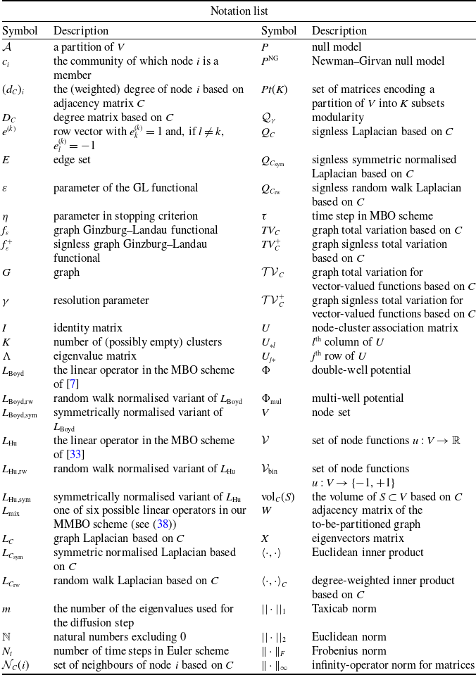
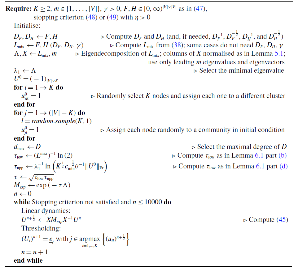
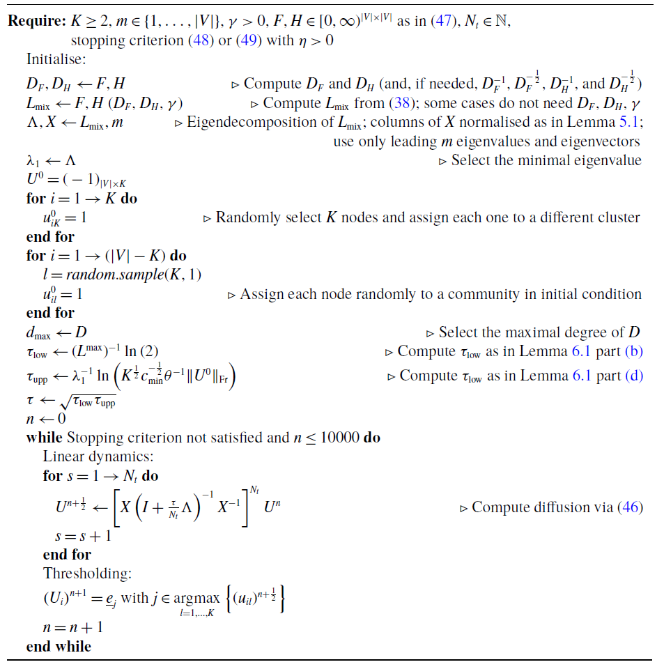
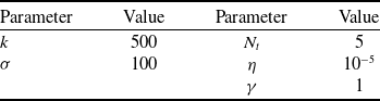
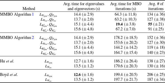


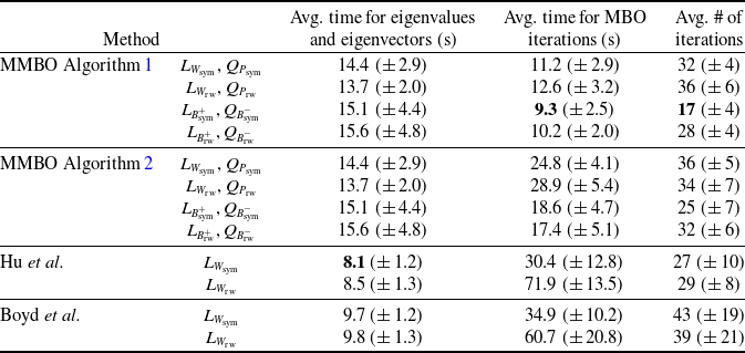


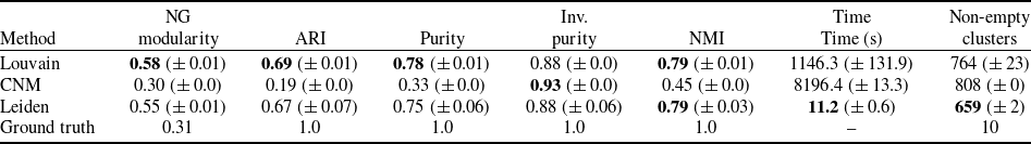
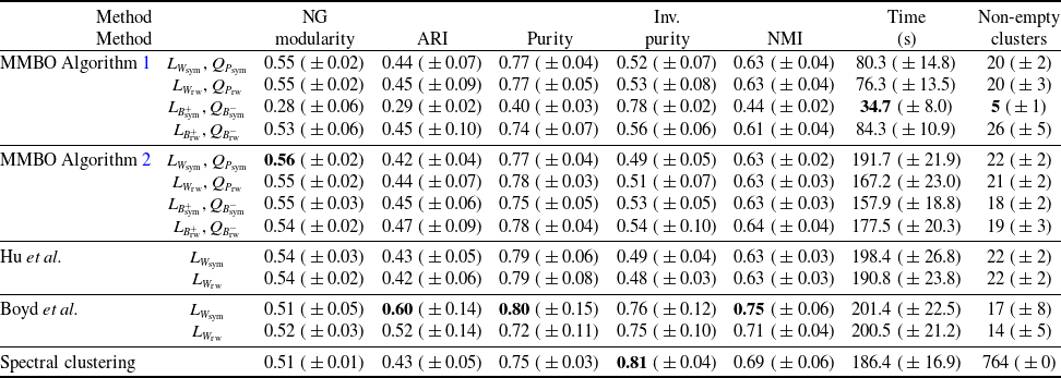


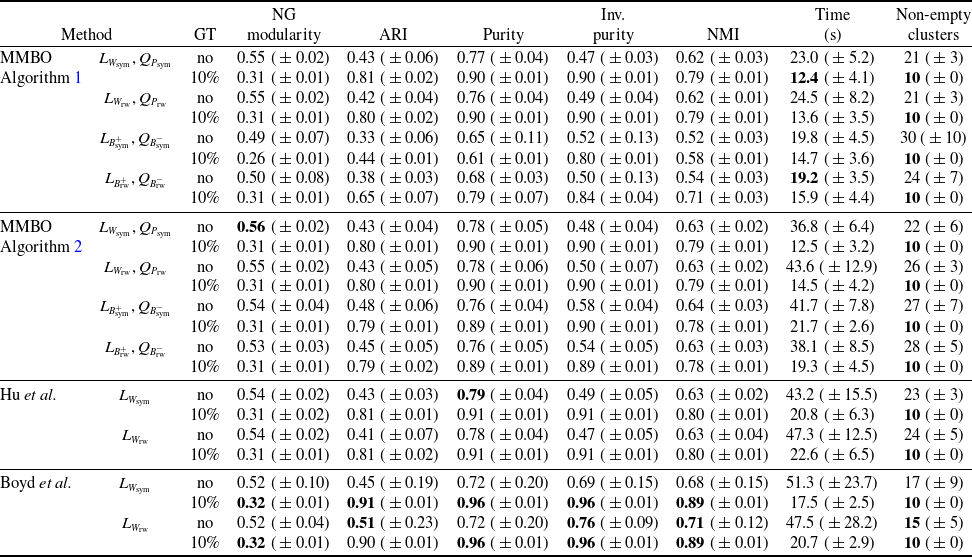


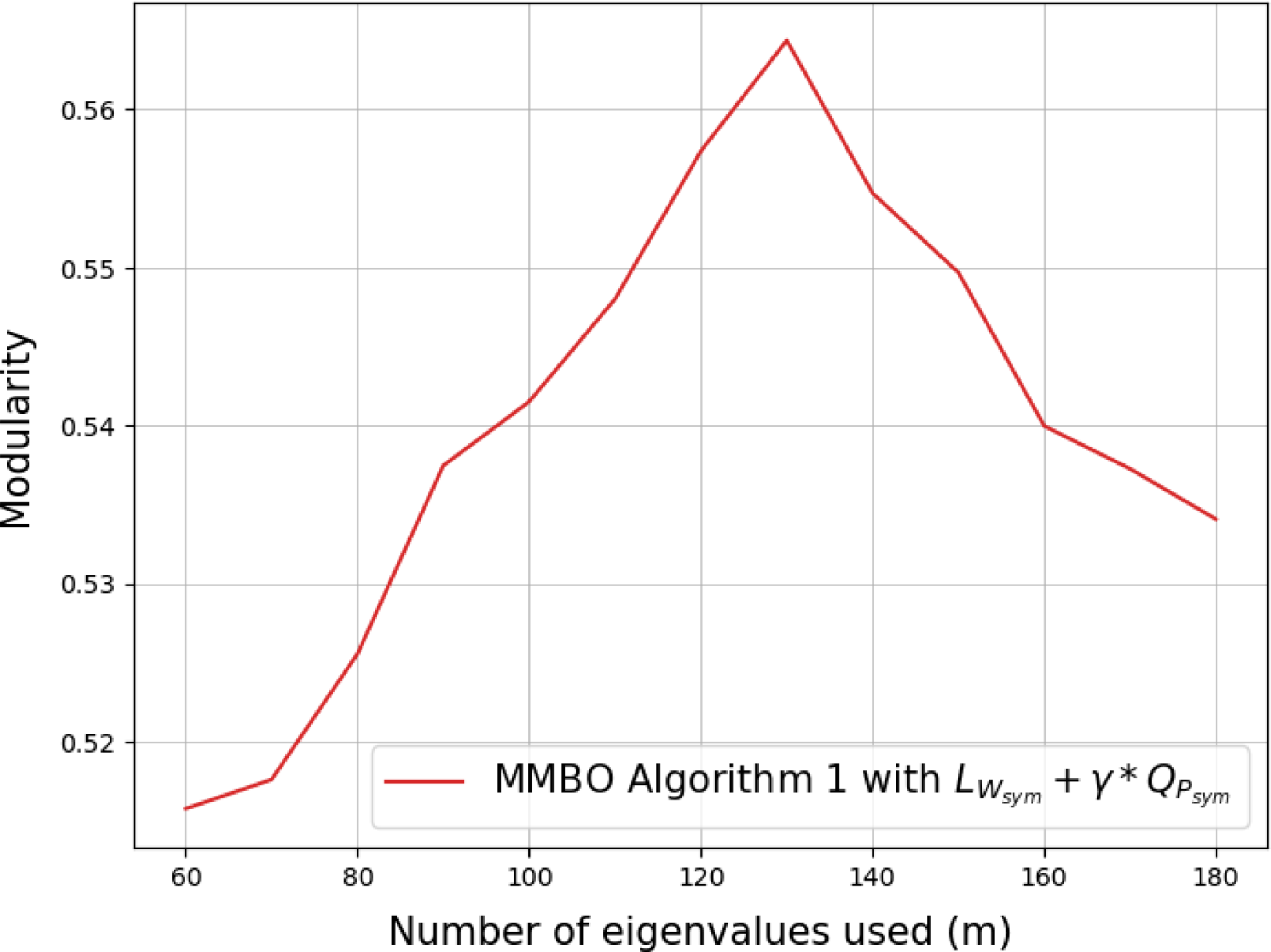


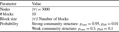


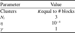


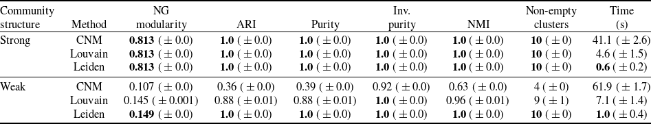


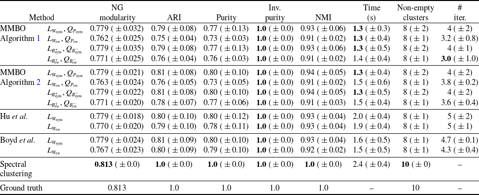


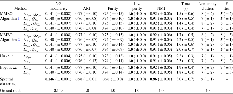


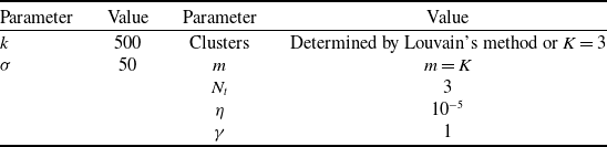
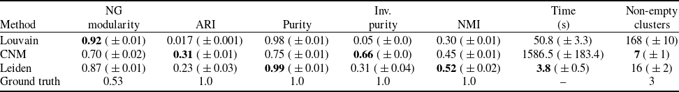

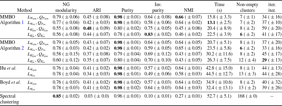


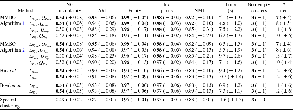


 Open access