


1. INTRODUCTION
The Greenland ice sheet has been losing mass at an increasing rate over the last decades (e.g., Vaughan and others, Reference Vaughan, Stocker, Qin, Plattner, Tignor, Allen, Boschung, Nauels, Xia, Bex and Midgley2013; Khan and others, Reference Khan2015). The mass loss is dominated by surface melt and ice discharge from marine-terminating outlet glaciers (Sasgen and others, Reference Sasgen2012; Enderlin and others, Reference Enderlin2014; Khan and others, Reference Khan2014; Mouginot and others, Reference Mouginot2015). While the general mass loss is triggered by increasing air and ocean temperatures, local/regional conditions determine its timing and pace. Observations have revealed that the mass loss was most pronounced in southeastern Greenland before ~ 2005, but migrated towards the northwest in the years thereafter (Kjær and others, Reference Kjær2012). This generally correlates with the acceleration, thinning and retreat of Greenland's marine-terminating outlet glaciers, which was first detected around the southeastern and southwestern edges of the ice sheet (Thomas and others, Reference Thomas2000; Joughin and others, Reference Joughin, Abdalati and Fahnestock2004; Howat and others, Reference Howat, Joughin, Tulaczyk and Gogineni2005, Reference Howat, Joughin and Scambos2007; Rignot and Kanagaratnam, Reference Rignot and Kanagaratnam2006; Nettles and others, Reference Nettles2008), but later spread towards the north (McFadden and others, Reference McFadden, Howat, Joughin, Smith and Ahn2011; Kjær and others, Reference Kjær2012; Moon and others, Reference Moon, Joughin, Smith and Howat2012).
The processes causing the observed glacier changes are still incompletely understood. Glacier and fjord bed geometry was suggested as a key factor controlling acceleration and rapid retreat (Schoof, Reference Schoof2007; Nick and others, Reference Nick, Vieli, Howat and Joughin2009). Ocean temperature is also likely an important factor, as exemplified by the effect of rising temperatures on the acceleration of Jakobshavn Isbræ during the 1990s (Holland and others, Reference Holland, Thomas, de Young, Ribergaard and Lyberth2008). Increased subaqueous melting under the influence of changing ocean conditions is suspected as an important process (e.g., Straneo and Heimbach, Reference Straneo and Heimbach2013; Rignot and others, Reference Rignot2016), and therefore, the fronts of calving glaciers and the nearby fjord areas have been the focus of several recent studies (e.g., Mankoff and others, Reference Mankoff2016; Jouvet and others, Reference Jouvet2018). Another important observation is short-term ice speed variations near the glacier front. Ice dynamics can vary on hourly to seasonal temporal scales under the influence of external forcing on the force balance (e.g., Podrasky and others, Reference Podrasky2012). Thus, these variations provide a clue to understanding the mechanisms of recent speed-up and rapid retreat of tidewater glaciers.
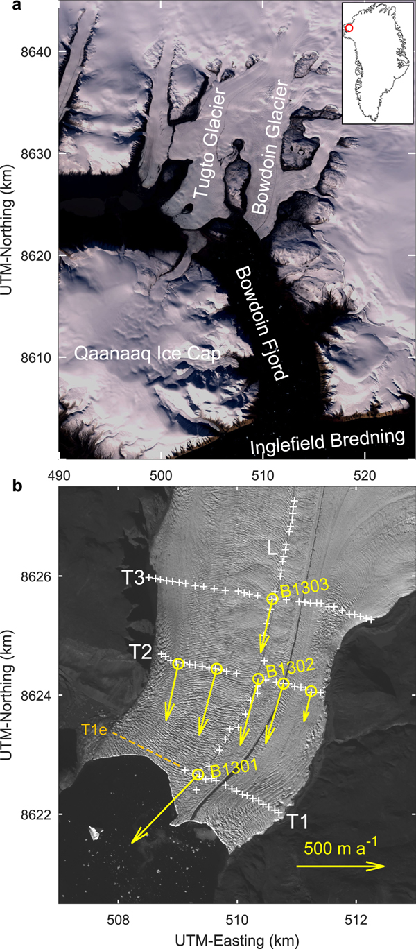
The Qaanaaq drainage basin, situated in the northwestern part of the Greenland ice sheet, is a typical Greenlandic drainage basin that consists of an inland accumulation area and a marginal ablation area with a number of fast-flowing outlet glaciers (e.g., Sakakibara and Sugiyama, Reference Sakakibara and Sugiyama2018). It was chosen as a focus area of Japanese glaciological research activities because of the observed increased mass loss in northwestern Greenland, and because it had been relatively unexplored before. Field and remote sensing activities have been carried out in the area since 2013 within the Green Network of Excellence (GRENE) Arctic Climate Change Research Project (www.nipr.ac.jp/grene) and the Arctic Challenge for Sustainability (ArCS) Project (www.arcs-pro.jp) (Sugiyama and others, Reference Sugiyama2017). One particular focus was Bowdoin Glacier, a fast-flowing outlet glacier terminating into Bowdoin Fjord (77°4′ N, 68°35′ W; Fig. 1a). For this glacier, satellite data show a relatively stable front position from 1987 to 2008, followed by a rapid retreat of more than 1 km between 2008 and 2013. This retreat correlates with atmospheric and ocean surface warming trends in the region (Sugiyama and others, Reference Sugiyama, Sakakibara, Tsutaki, Maruyama and Sawagaki2015; Sakakibara and Sugiyama, Reference Sakakibara and Sugiyama2018). During a field campaign in summer 2013, ice speed measurements were carried out on Bowdoin Glacier by surveying poles installed at seven locations on the glacier surface (yellow circles in Fig. 1b) with GPS receivers. Short-term speed variations were found, correlating with air temperature and precipitation on the synoptic time scale, and with the semi-diurnal ocean tides. These observations led to the assumption that the glacier flow is sensitive to (1) water input at the surface rapidly drained to the bed, resulting in basal lubrication, and (2) changes in the force balance at the calving front (Sugiyama and others, Reference Sugiyama, Sakakibara, Tsutaki, Maruyama and Sawagaki2015).
(a) Location of Bowdoin Glacier in the Qaanaaq region, northwestern Greenland (Landsat image, 23 August 2013). The inset shows the location of the study site in Greenland. (b) Satellite image from ALOS (Japanese Advanced Land Observing System) PRISM (Panchromatic Remote-sensing Instrument for Stereo Mapping), 25 July 2010, showing the location of the measurement sites for ice radar (white crosses) and surface velocity (yellow circles). The radar profiles are labelled by L (longitudinal) and T1–T3 (transversal) [note that we refer to T1 by T1e when extended across the entire width of the glacier]. Yellow arrows represent the surface velocities measured between 13 and 26 July 2013 (B1301: only between 13 and 21 July). Figure panels modified from Sugiyama and others (Reference Sugiyama, Sakakibara, Tsutaki, Maruyama and Sawagaki2015).

Models with various levels of sophistication have been applied to Greenland's ice streams and outlet glaciers (e.g., Nick and others, Reference Nick, Vieli, Howat and Joughin2009; Van der Veen and others, Reference Van der Veen, Plummer and Stearns2011; Vieli and Nick, Reference Vieli and Nick2011; Nick and others, Reference Nick2013; Krug and others, Reference Krug, Weiss, Gagliardini and Durand2014; Larour and others, Reference Larour2014; Todd and Christoffersen, Reference Todd and Christoffersen2014; Krug and others, Reference Krug, Durand, Gagliardini and Weiss2015; Schlegel and others, Reference Schlegel, Larour, Seroussi, Morlighem and Box2015; Choi and others, Reference Choi, Morlighem, Rignot, Mouginot and Wood2017), and the findings advanced our understanding of their dynamics and response to climate change significantly. However, the majority of models used were two-dimensional flowline models or did not employ the full-Stokes approach (retaining all stress components in the force balance), which, to some extent, limits the interpretability of the results. Two recent studies, both carried out with the three-dimensional version of the full-Stokes model Elmer/Ice (Zwinger and others, Reference Zwinger, Greve, Gagliardini, Shiraiwa and Lyly2007; Gagliardini and others, Reference Gagliardini2013), focused on the relation between calving and internal dynamics for Bowdoin Glacier (Jouvet and others, Reference Jouvet2017) and Store Glacier (Todd and others, Reference Todd2018).
In this study, we use the model Elmer/Ice to investigate the influence of short-term external forcings on the flow dynamics of Bowdoin Glacier. First, we apply a control inverse method to infer the basal drag based on the observed surface velocities, and we compute the present-day temperature field in the glacier. Motivated by the observations reported above, we then conduct experiments to assess the sensitivity of Bowdoin Glacier to (1) basal lubrication, or reduced basal friction (due to surface melting or precipitation events), and (2) changing hydrostatic pressure acting on the calving front (due to the semi-diurnal ocean tides). Since, in the full-Stokes formulation, the viscous response of the glacier is instantaneous and notable changes in topography and englacial temperature are not to be expected on the short time scales considered here, we limit ourselves to diagnostic (time-independent) simulations in which momentary situations are analysed.
2. METHODS
2.1. Modelling approach
The main tool for this study is the ice sheet and glacier model Elmer/Ice (Zwinger and others, Reference Zwinger, Greve, Gagliardini, Shiraiwa and Lyly2007; Gagliardini and others, Reference Gagliardini2013) in full-Stokes mode. The dynamic/thermodynamic field equations and boundary conditions are described elsewhere (Gagliardini and others, Reference Gagliardini2013; Seddik and others, Reference Seddik, Greve, Zwinger and Sugiyama2017). The physical parameters, listed in Table 1, follow closely those used by Seddik and others (Reference Seddik, Greve, Zwinger and Sugiyama2017). The exception is the flow enhancement factor, for which we use the value E=3 as a compromise between the values 2 and 5 recommended by Cuffey and Paterson (Reference Cuffey and Paterson2010) for Holocene and ice-age Arctic ice, respectively.
Standard physical parameters used for the simulations with Elmer/Ice (largely following Seddik and others, Reference Seddik, Greve, Zwinger and Sugiyama2017)
At the glacier bed, we apply a linear sliding law that relates the basal shear stress to the basal velocity:
 $${{\bi t}^{\bf {\rm T}}} \cdot {\bf {\rm T}} \cdot {\bi n} + \beta {\bi v} \cdot {\bi t}= 0,$$
where T is the Cauchy stress tensor,  ${\bi v}$ the velocity vector, β the basal friction coefficient to be computed with the control inverse method (see below), ${\bi n}$ the outer normal unit vector and ${\bi t}$ the tangential unit vector.
The control inverse method was introduced by MacAyeal (Reference MacAyeal1993) and implemented in Elmer/Ice by Gillet-Chaulet and others (Reference Gillet-Chaulet2012). The description below follows Seddik and others (Reference Seddik, Greve, Zwinger and Sugiyama2017) very closely. The method is based on the computation of the full-Stokes adjoint (Morlighem and others, Reference Morlighem2010) and the definition of a cost function J 0 that is expressed as the difference between the norm of the modelled and observed horizontal velocities ( ${\bi v}_{\bf {\rm h}}$ and ${\bi v}_{{\rm h}}^{{\rm obs}}$, respectively):
 $$J_{\rm 0} = \int_{\Gamma _{\rm s}} {\displaystyle{1 \over 2}{(\vert{\bi v}_h\vert-\vert{\bi v}_h^{{\rm obs}} \vert)}^2{\rm d}\Gamma ,} $$
where Γsis the footprint of the glacier surface in the x–y plane. The regularization procedure is constructed by adding a smoothness constraint to the cost function in the form of a Tikhonov regularization term,
 $$J_{{\rm reg}} = \displaystyle{1 \over 2}\int_{\Gamma_{\rm b}\,} {{\bigg ({\Big (}\displaystyle{{\partial \alpha } \over {\partial x}}{\Big )}}^2{\rm + }\,{{\Big (}\displaystyle{{\partial \alpha } \over {\partial y}}{\Big )}}^2\bigg )\,{\rm d\Gamma }},$$
where Γb is the footprint of the glacier bed in the x–y plane. The parameter α is used to avoid negative values of the basal friction coefficient β and is defined as
 $$\beta = 10^{\alpha}. $$
The total cost function is then given by
 $$J_{{\rm tot}} = J_0 + \lambda J_{{\rm reg}},$$
where λ is the positive regularization parameter. We use the quasi-Newton routine M1QN3 to minimize the cost function J tot with respect to α (Gilbert and Lemaréchal, Reference Gilbert and Lemaréchal1989; Gillet-Chaulet and others, Reference Gillet-Chaulet2012).
2.2. Computational domain
2.2.1. Surface topography
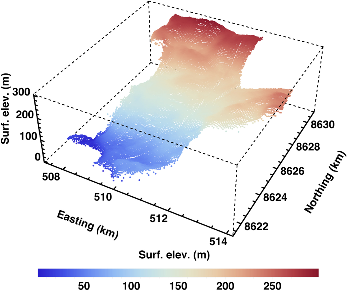
We generated a digital elevation model (DEM) for the surface of Bowdoin Glacier and its tributary based on imagery from the Advanced Land Observing Satellite (ALOS) Panchromatic Remote-sensing Instrument for Stereo Mapping (PRISM) (2.5 m resolution) acquired on 4 September 2010. Stereo pair images were processed with the digital photogrammetry software Leica Photogrammetric Suite 2011, mounted on an ERDAS IMAGINE 2011 workstation. To improve accuracy, the automatically generated elevation data were manually corrected by viewing a stereoscopic glacier image on a stereo monitor (PLANAR SD 2020 Stereo MirrorTM/3D Monitor). The achieved accuracy, estimated by the standard deviation of elevation differences in ice-free terrain between ALOS DEM and GPS kinematic survey, is ± 3.4 m (Tsutaki and others, Reference Tsutaki, Sugiyama, Sakakibara and Sawagaki2016). For this study, we interpolated the non-uniformly distributed elevation data on a regular grid with a resolution of 50 m. The resulting DEM is shown in Figure 2.
Surface DEM of Bowdoin Glacier and its tributary derived from the ALOS imagery. Projection: UTM (grid zone 19N).
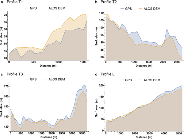
In Figure 3, we compare the DEM with surface-based observations by kinematic GPS along the profiles T1, T2, T3 and L (Fig. 1b). The agreement is generally good down to structures on the 100 m scale. The biggest differences occur near the glacier front (profile T1, Fig. 3a), where the ALOS surface DEM is systematically higher than the elevation profile derived from the surface-based measurements. This is so because the ALOS imagery predates the surface-based measurements by several years, and the thinning rate of the glacier is largest in the region near the front. The root-mean-square deviation (RMSD) between the ALOS DEM and the GPS observations along the four profiles is 5.94 m.
Comparison between the surface DEM derived from the ALOS imagery (Fig. 2) and the surface elevations measured by kinematic GPS along the ice radar profiles shown in Figure 1b: (a) profile T1, (b) profile T2, (c) profile T3, (d) profile L. Distances along T1–T3 measured from WNW to ESE, along L upstream from the glacier front. Note the different scales of the axes.

2.2.2. Bedrock topography
In order to create the bedrock topography underneath Bowdoin Glacier, we first interpolated the bed elevation dataset for Greenland by Bamber and others (Reference Bamber2013) on the same 50 m grid we used for the surface DEM. The resulting bedrock topography is relatively high upstream of the confluence with the tributary, then changes to a deep trough and rises again towards the glacier front (not shown). The deepest section near the middle part of the glacier and on its tributary coincides with the CReSIS00 flight tracks (Gogineni and others, Reference Gogineni2001; Bamber and others, Reference Bamber2013), which indicates that these regions are well reproduced. By contrast, preliminary tests with Elmer/Ice have shown that the upstream area is too shallow to allow reproducing the order of magnitude of the observed surface velocities, and in the downstream area, there are very substantial disagreements (hundreds of metres) with the radar measurements along the profiles shown in Figure 1b (Sugiyama and others, Reference Sugiyama, Sakakibara, Tsutaki, Maruyama and Sawagaki2015).
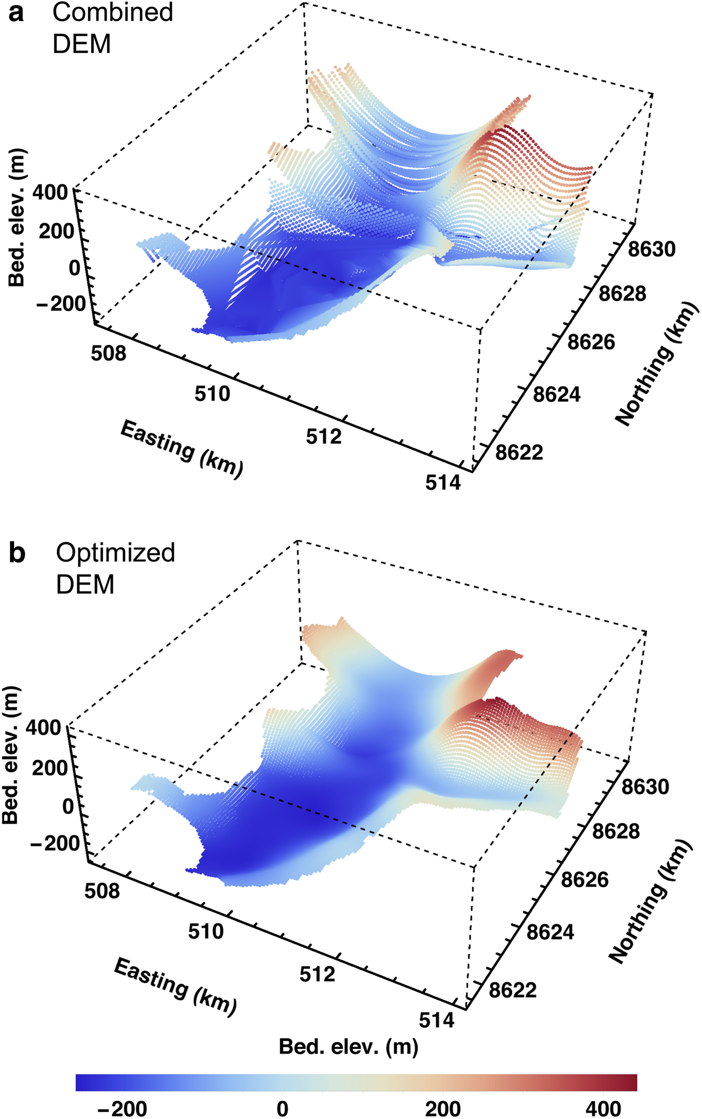
Therefore, we employ an optimization procedure that combines three different datasets. For the interior part of the glacier and the tributary, we stick to the data by Bamber and others (Reference Bamber2013). Further downstream (towards the glacier front), we interpolated the ice radar and sea-bed elevation data acquired from the fjord near the glacier front (Sugiyama and others, Reference Sugiyama, Sakakibara, Tsutaki, Maruyama and Sawagaki2015) on our grid. For the upstream part of the glacier, no detailed observational data are available. We assumed a parabolic cross-section everywhere in this area and constructed 53 parabolas based on three nodes each. Two of the nodes of each parabola are margin points of the glacier with zero thickness (thus the bedrock elevation equals the known surface elevation). The third node is in the centre of the glacier, where the thickness is assumed to be equal to the maximum ice thickness in the area further downstream where we use the data by Bamber and others (Reference Bamber2013). The computed parabolas were assembled with the rest of the bedrock topography (Fig. 4a). In the last step, a kernel average smoother was applied to eliminate discontinuities within the domain. The resulting bedrock DEM is shown in Figure 4b.
Bedrock DEM of Bowdoin Glacier and its tributary. (a) After combining the data by Bamber and others (Reference Bamber2013) (interior and tributary), Sugiyama and others (Reference Sugiyama, Sakakibara, Tsutaki, Maruyama and Sawagaki2015) (downstream area) and the parabolic cross-sections (upstream area). (b) Final, optimized DEM after smoothing. Projection: UTM (grid zone 19N).
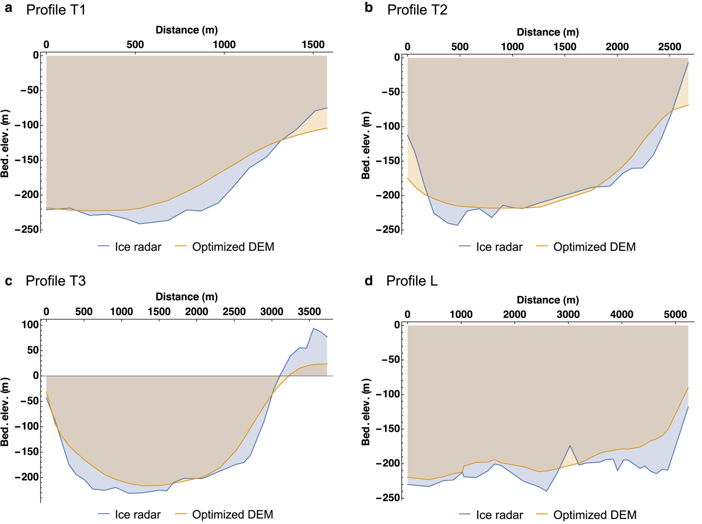
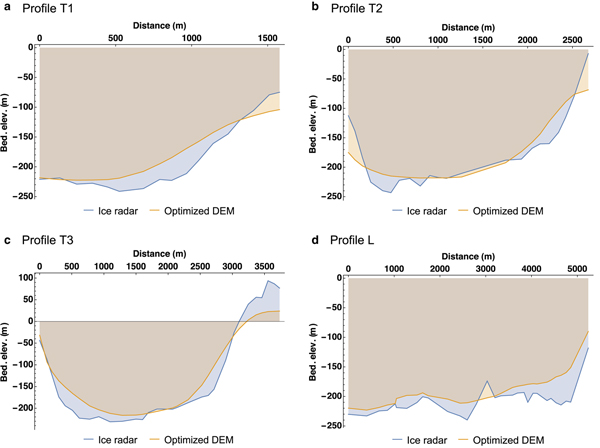
In Figure 5, we verify the quality of the optimized bedrock DEM by comparison with the ice radar data obtained along the profiles T1, T2, T3 and L. Even though some of the fine structures of the radar profiles were lost, the general shape is reproduced well. The RMSD between the DEM and the radar observations along the four profiles is 26.43 m. Together with the RMSD of the surface DEM (see above), this leads to an ice thickness error of ~ 30 m. Since typical ice thicknesses of the glacier are in the range of 200–300 m, the resulting relative error is ~ 10–15%.
Comparison between the bedrock DEM obtained by the optimization procedure (Fig. 4b) and the bedrock elevations measured along the ice radar profiles shown in Figure 1b: (a) profile T1, (b) profile T2, (c) profile T3, (d) profile L. Distances along T1–T3 measured from WNW to ESE, along L upstream from the glacier front. Note the different scales of the axes.
2.3. Meshing and numerical methods
The finite element mesh for the domain was created by building a two-dimensional footprint, which was meshed using triangular elements with a constant horizontal resolution of 70 m. The three-dimensional mesh was then obtained by vertical extrusion of the footprint, using 11 equidistant, terrain-following layers bounded by the surface and bedrock DEMs (Figs 2 and 4b). A minimum ice thickness of 10 m was assumed everywhere in the domain for reasons of numerical stability. The resulting three-dimensional mesh consists of 228 044 prismatic elements.
While the construction of the surface and bedrock DEMs was done based on a UTM projection (grid zone 19N) for convenience, we use a polar stereographic projection with standard parallel at 71°N and central meridian at 39°W (Bamber and others, Reference Bamber2013) for the numerical simulations. We set up a Cartesian coordinate system in which x and y span the horizontal (stereographic) plane, and z points upward.
The non-linearity of the model equations is dealt with by initially performing some Picard iterations (until the RMSD between the previous and current velocity fields of the non-linear iteration loop falls below a prescribed threshold), and then activating the Newton linearization (Gagliardini and others, Reference Gagliardini2013). The stabilization method by Franca and others (Reference Franca, Frey and Hughes1992) and Franca and Frey (Reference Franca and Frey1992) is applied to the finite element discretization. The resulting system of linear equations is solved with a direct method using the parallel sparse direct solver MUMPS (Amestoy and others, Reference Amestoy, Duff, Koster and L'Excellent2001, Reference Amestoy, Guermouche, L'Excellent and Pralet2006).
3. NUMERICAL EXPERIMENTS
First, we compute reference conditions for the velocity and temperature fields of Bowdoin Glacier. In order to obtain a numerically stable solution, the following sequence is employed:
1. The velocity field is computed preliminarily by using a constant viscosity (Newtonian fluid) of 1015 Pa s, a no-slip condition at the glacier base and a zero-velocity condition at the upstream inflow boundaries of the main glacier and the tributary. At the grounded glacier front, the stress is given by the hydrostatic pressure exerted by the sea water at the mean tide level.
2. Starting from the velocity field obtained in step (1) and assuming isothermal conditions (− 10°C everywhere in the glacier), the velocity field is re-computed by using Glen's flow law with the parameters specified in Table 1. Boundary conditions like in step (1). The temperature field is then computed by applying Dirichlet-type boundary conditions at the surface and the glacier base. The surface temperature over the entire domain is set to the mean annual air temperature in the region at sea level, which is − 8°C (Sugiyama and others, Reference Sugiyama2014). The glacier base is assumed to be temperate, that is, the basal temperature is set to the pressure melting point everywhere. At the upstream inflow boundaries and the downstream glacier front, we assume a zero-gradient condition.
3. Starting from the results of step (2), a fully coupled steady-state solution for the velocity and temperature fields is computed with boundary conditions as described above.
4. Starting from the results of step (3) and a constant value of the basal friction coefficient, βinit = 10−4 MPa m−1 a, the control inverse method (Section 2.1) is used to compute the distribution of the basal friction coefficient β. The observed horizontal surface velocity field ${\bi v}_{\rm {h}}^{\rm {obs}}$ used for the inversion is the annual mean for 2013, measured by applying an image-matching technique to satellite imagery (Sugiyama and others, Reference Sugiyama, Sakakibara, Tsutaki, Maruyama and Sawagaki2015). These surface velocities are prescribed at the upstream inflow boundaries, and the temperature field is kept unchanged.
5. The temperature field is recomputed with the velocity field obtained from the inversion by a transient run over 1000 years. In order to preserve numerical stability, a zero-velocity condition is used at the upstream inflow boundaries.

We refer to the above sequence as the control experiment (CTL). The resulting velocity and temperature fields are used to initialize a series of diagnostic sensitivity experiments. These are motivated by the following observations at Bowdoin Glacier (Sugiyama and others, Reference Sugiyama, Sakakibara, Tsutaki, Maruyama and Sawagaki2015): (i) the ice flow appears to respond to surface temperature rise and heavy rain events, indicating a rapid drainage of surface water to the glacier bed; (ii) the semi-diurnal maxima of the ice flow appear to coincide with low tides, suggesting a significant influence of the changing hydrostatic pressure acting on the glacier front. Therefore, we investigate the response of the glacier to basal lubrication and to ocean tides:
Experiments BP: Basal perturbation (BP) by increasing basal lubrication. Since we do not model englacial water transport and basal hydrology in this study, we cannot estimate a-priori the amount of basal lubrication that results from a certain amount of water input at the surface. Therefore, we implement basal lubrication in an ad-hoc way by reducing the basal friction coefficient β everywhere in the domain by 10% (BP1), 20% (BP2), 30% (BP3) and 40% (BP4). The sea level is the same as in the control run. We will see in Sections 4.2 and 4.3 that the chosen range of reductions covers the observed speed-up events of the glacier.
Experiments ST: Effect of ocean tides. Sugiyama and others (Reference Sugiyama, Sakakibara, Tsutaki, Maruyama and Sawagaki2015) presented the ocean tide signal at Pituffik/Thule (76°33′ N, 68°52′ W) for the period 6–27 July 2013. Measurements near the glacier front carried out in July 2016 (M. Minowa, unpublished) show that the tidal signal at Bowdoin Glacier is in phase with the signal at Pituffik/Thule, but larger by a factor 1.18 (with a coefficient of determination r 2 = 0.98). This leads to a tidal amplitude of ~ 1.5 m (shown below in Fig. 11). We sample this range by lowering the sea level by 2 m (ST1), 1.5 m (ST2), 1 m (ST3) and 0.5 m (ST4), and raising it by 0.5 m (ST5), 1 m (ST6), 1.5 m (ST7) and 2 m (ST8). The basal friction coefficient β is the same as in the control run.
The ST experiments are further used as control points to compute by interpolation the semi-diurnal flow variability that results from the tidal forcing at the glacier front.
4. RESULTS AND DISCUSSION
4.1. Control experiment
As described above, we used the control inverse method to compute the spatial distribution of the basal friction coefficient that leads to an optimum match between observed and computed surface velocities. The parameter λ in Eqn (5) was chosen by the L-curve method (Hansen, Reference Hansen and Johnston2001; Gillet-Chaulet and others, Reference Gillet-Chaulet2012; Seddik and others, Reference Seddik, Greve, Zwinger and Sugiyama2017). The L-curve depicts the regularization term J reg (a measure of the roughness of the distribution of the basal friction coefficient) as a function of the mismatch term J 0 in Eqn (5). It is shown in Figure 6. When increasing λ from 0 to 107, the roughness J reg decreases by several orders of magnitude, and the mismatch J 0 decreases slightly. For higher values of λ (108 and more), the distribution of the basal friction coefficient becomes too smooth, hence the mismatch J 0 increases. The optimal value of λ was therefore chosen as λ = 107.
L-curve obtained with the control inverse method: Cost function J 0 and Tikhonov regularization term J reg, parameterized by the regularization parameter λ (see Eqn (5)).

Figure 7 shows a comparison between the observed velocities (panel a) and the velocities obtained by the control inverse method (panel b). Overall, the agreement is very good, and the zones of fast and slow flowing ice are generally well reproduced. The RMSD of the simulated velocities over the entire domain is 25.02 m a−1. The most notable discrepancy occurs in the centre of the upstream area, where the model produces by > 50 m a−1 too large velocities. This is most likely caused by the large uncertainties of the bedrock topography in this area, where we assumed parabolic cross-sections with constant thickness (Section 2.2.2). This might lead to an overestimation of the ice thickness in the area and thus a too large driving stress. Near the side margins of the glacier, the simulated velocities are consistently too small, often by > 50 m a−1. This is probably due to small ice thicknesses that entail large relative errors of the ice thickness, and further due to uncertainties of the observed velocities close to the margins. Near the glacier front, the disagreement pattern is patchy, the observed field showing more fine structure than the simulated one, which is smoother due to the regularization of the inverse method. A further possible reason for disagreements between observed and simulated velocities is the fact that our surface DEM is from 2010, whereas the velocity data are from 2013. This time difference is unavoidable because the DEM is exclusively available for 2010, while we only have a useful velocity map with good coverage for 2013.
Control experiment (CTL): (a) observed surface velocities (Sugiyama and others, Reference Sugiyama, Sakakibara, Tsutaki, Maruyama and Sawagaki2015), (b) computed surface velocities, (c) basal friction coefficient β, and (d) slip ratio (ratio of basal to surface velocities). Projection: polar stereographic (Section 2.3).
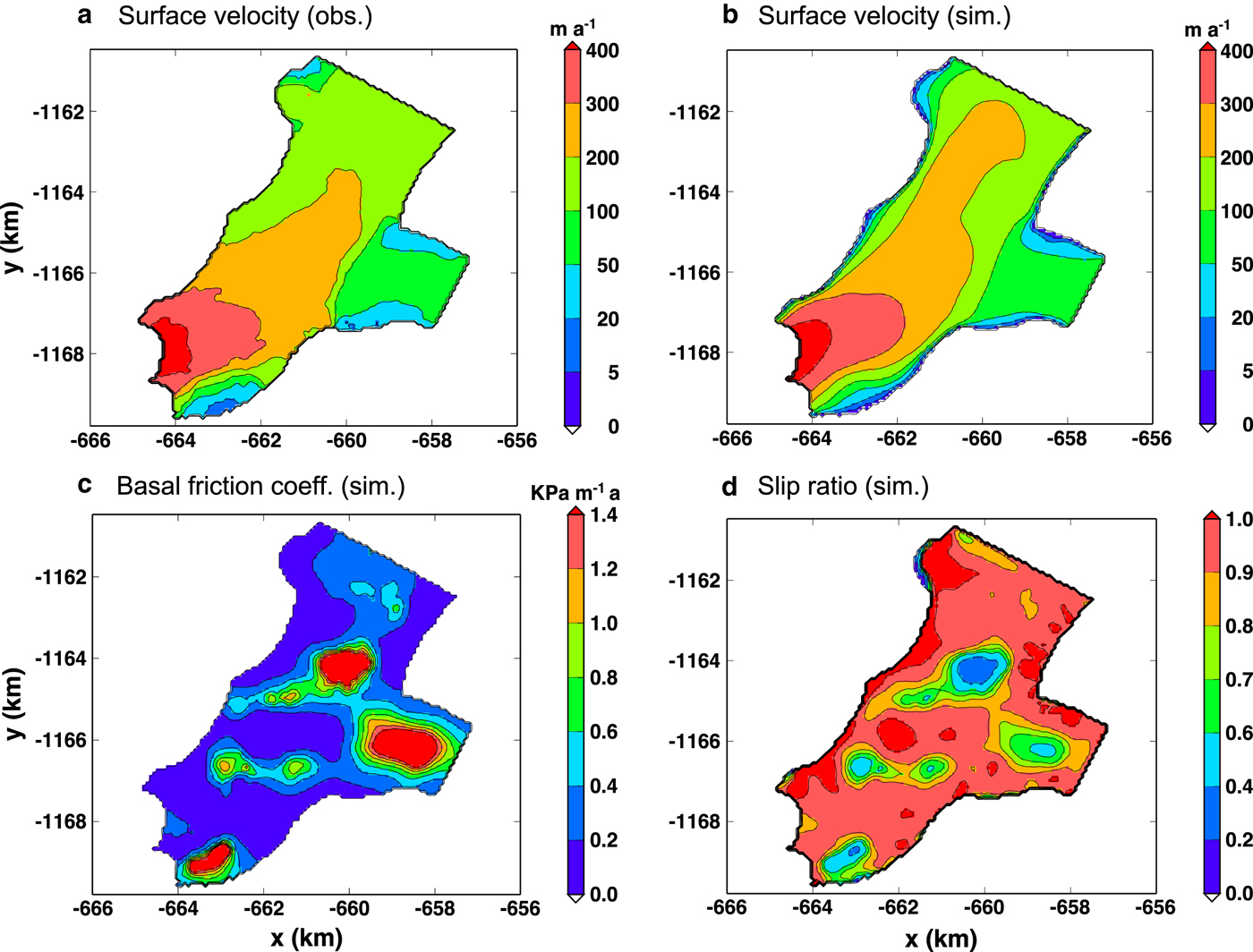
The distribution of the computed basal friction coefficient and the ratio of basal to surface velocities (slip ratio) are shown in Figure 7 (panels c and d). These two quantities are closely related, such that low friction coefficients correspond to high slip ratios, and vice versa. Most areas of the glacier are characterized by near-plug-flow conditions with low basal friction and slip ratios between 0.9 and 1. However, the inversion also produces three major and several minor sticky spots with enhanced basal drag. One of the major sticky spots is situated in the eastern part of the glacier near the calving front, and it is responsible for the low velocities found there. It coincides with a shallow bed topography near the eastern glacier margin (Fig. 5a), an elevated surface geometry (Fig. 3a) and an unusual, irregular crevasse pattern (Fig. 1b) that might indicate an area of increased basal roughness. The second major spot is in the centre of the tributary, and it is required to keep the flow velocities limited. The third major spot, upstream of the confluence of the main glacier and its tributary, features the lowest slip ratios. However, as discussed above, the bedrock topography is quite uncertain in this area, so that we cannot exclude the possibility that this structure is merely a modelling artefact.
The stress regime of Bowdoin Glacier is illustrated in Figure 8. It shows the main components of the deviatoric stress tensor (Cauchy stress tensor T without the contribution from the pressure that does not contribute to ice deformation) in the T1e profile (an extended T1 profile across the entire width of the glacier) near the calving front. Note that, for this purpose, we use a rotated coordinate system in which x is perpendicular to T1e (approximately in the flow direction), and y is parallel to it. The horizontal normal deviatoric stress  $\tau _{xx}^{\rm D}$ (panel a) generally decreases from the surface to the base. It is tensile (> 0) in the inner part of the glacier, but compressive (< 0) near the margin on both sides. The vertical normal deviatoric stress $\tau _{zz}^{\rm D}$ (panel b) shows essentially the opposite behaviour, and both add up approximately to zero in most of the transect. Consequently, the lateral component $\tau _{yy}^{\rm D}$ (not shown) is small. The horizontal shear stress τ xy (panel c) originates mainly from side drag. It should therefore be largest near both margins. This holds true for the western margin (largest positive values), while the largest negative values occur at some distance from the eastern margin. The likely reason for this is the sticky spot near the eastern margin already discussed above, which produces low velocities and moves the active shear zone towards the interior of the glacier. The vertical shear stress τ xz (panel d) is very small near the surface and increases downward, which is due to the basal drag. Therefore, rather large values are found near the eastern margin in the area where the sticky spot is situated.
Stress components resulting from the control experiment (CTL) at the profile T1e: (a) horizontal normal deviatoric stress  $\tau _{xx}^{\rm D}$, (b) vertical normal deviatoric stress $\tau _{zz}^D $, (c) horizontal shear stress τ xy, (d) vertical shear stress τ xz (coordinates x and y rotated such that x is perpendicular to T1e, and y is parallel to it). Distance along T1e measured from WNW to ESE.
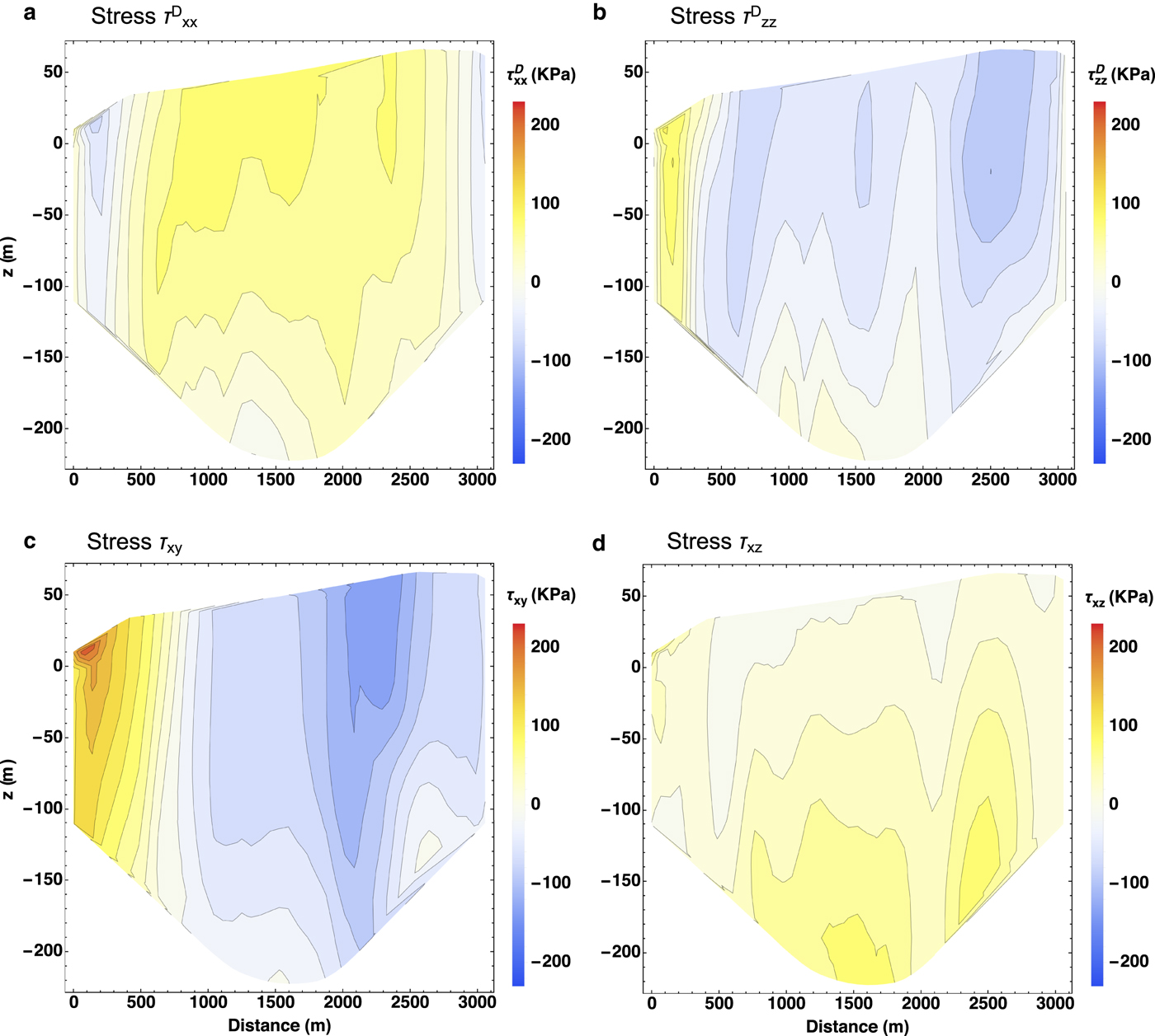
All stress components are of the same order of magnitude. Therefore, the near-frontal part of Bowdoin Glacier is characterized by a complex stress regime that is best modelled by the full-Stokes approach (as we did). The shallow ice approximation that has widely been used for describing large-scale ice sheet flow, and sometimes even for smaller glaciers (e.g., Blatter and others, Reference Blatter, Greve and Abe-Ouchi2011), retains only the vertical shear stress, but neglects all normal stress deviators and the horizontal shear stress. This approximation would evidently be inappropriate for our problem.
4.2. Sensitivity experiments
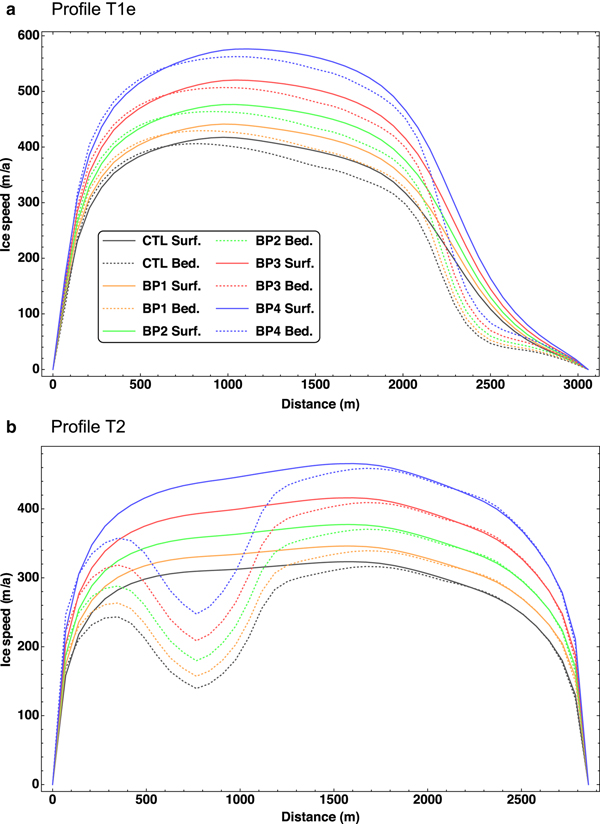
Figure 9 shows the computed surface and basal velocities for the control (CTL) and BP experiments at the transverse profiles T1e and T2. As to be expected, the glacier flow reacts strongly to the tested 10–40% range of reduction of the basal friction. The relative sensitivity (ratio of the speed-up to the CTL velocity) is slightly smaller for T1e (near the glacier front) than for T2 (further upstream), and it is about the same across the width of the glacier.
Sensitivity of the surface (“Surf.”) and basal (”Bed.”) velocities to changes of the basal lubrication (BP experiments) for (a) profile T1e and (b) profile T2. Distances along T1e and T2 measured from WNW to ESE.
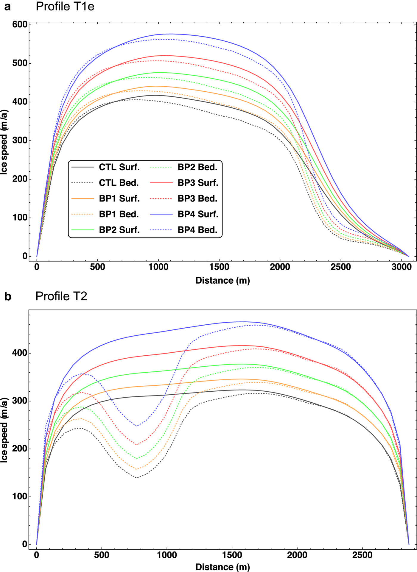
Both profiles cross one of the sticky spots visible in Figures 7c, d. In case of T1e, it is located near the eastern margin, while for T2, it is in the western part of the transect. These sticky spots manifest themselves by strong drops in the basal velocity, accompanied by mild drops in the surface velocity. The sensitivity to the reduction of the basal friction is not affected strongly by the presence of the sticky spots.
Observations for the period from 6 to 27 July 2013 showed speed-ups by ~ 7–50% at the site B1301 (Fig. 1b) during events of rising air temperature and precipitation (Sugiyama and others, Reference Sugiyama, Sakakibara, Tsutaki, Maruyama and Sawagaki2015). This agrees roughly with our modelled response of the glacier flow for the tested range of reduction of the basal friction. Therefore, a plausible explanation for the observed speed-up events is that the additional water input at the surface (due to either melting or rainfall) penetrates to the bed and leads to a temporarily increased basal lubrication. A quantitative connection between the amount of water input at the surface and the reduction of the basal friction would, of course, be desirable. However, this would require a detailed model of englacial water transport and basal hydrology, which is not part of the current study.
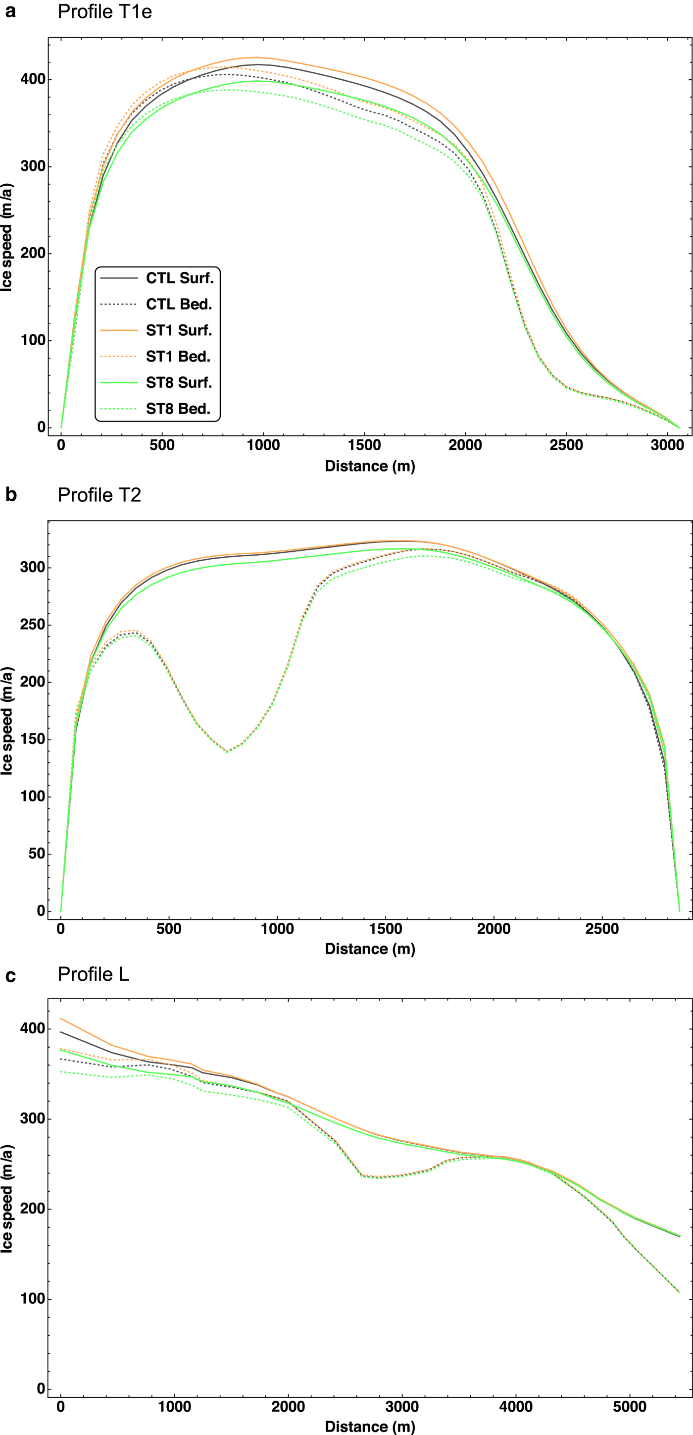
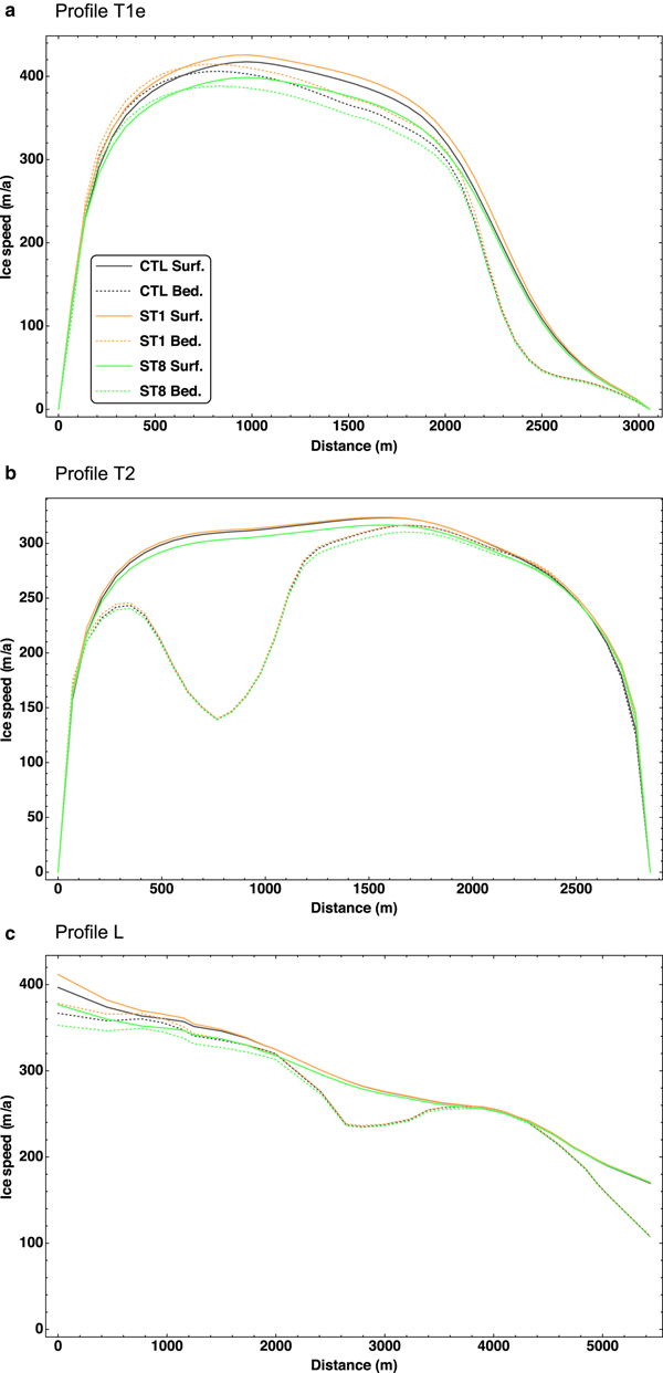
Figure 10 shows the computed surface and basal velocities for the control (CTL) experiment and the two extreme ocean-tide experiments ST1 (− 2 m) and ST8 (+ 2 m) at the transverse profiles T1e and T2 as well as the longitudinal profile L. The sensitivity of the glacier flow to these changes is smaller than to the above-discussed changes in the basal friction, but still significant. As expected, ST1 produces a speed-up, while ST8 produces a slow-down. The response is clearly more pronounced for T1e (near the glacier front) than for T2 (further upstream). This is highlighted further by the velocities along the profile L. The response to the tidal changes is strongest directly at the calving front, but declines to almost zero a few kilometres upstream.
Sensitivity of the surface (“Surf.”) and basal (“Bed.”) velocities to changes of the sea level (ST experiments) for (a) profile T1e, (b) profile T2 and (c) profile L. Distances along T1e and T2 measured from WNW to ESE, along L upstream from the glacier front.
4.3. Response to time-dependent tidal forcing
We now use the results of the ST experiments to compute the flow variability due to the time-dependent tidal forcing at the glacier front. Since, in the full-Stokes formulation, the velocity field reacts instantaneously to changes of the boundary conditions, we do this by interpolating the results from the diagnostic ST experiments on the tidal forcing. As stated in Section 3, we reconstruct the tidal signal at the front of Bowdoin Glacier from the one at Pituffik/Thule for the period 7–12 July 2013. The resulting semi-diurnal signal is shown in Figure 11 (blue dashed line).
Blue dashed line: Tidal forcing at the glacier front (see main text for details). Black solid line: Observed ice flow speed at site B1301 (Sugiyama and others, Reference Sugiyama, Sakakibara, Tsutaki, Maruyama and Sawagaki2015). Red solid line: Computed ice flow speed at site B1301 (by interpolating the results of the ST experiments). Green, cyan, magenta and orange solid lines: Same, but with the basal friction coefficient β reduced by 10, 20, 30 and 40%, respectively. Time axis: 7–12 July 2013.

The red and black lines in Figure 11 show the computed and observed flow speeds, respectively, at the site B1301 located near the glacier front (Fig. 1b). While the mean observed speed is ~ 1.35 m d−1, the mean computed speed is ~ 1.05 m d−1, thus some 20% smaller. The phase of the observed and simulated semi-diurnal speed variability agrees very well, and both are in anti-phase with the tidal forcing (high tide corresponds to low speed, and vice versa). By contrast, the model underpredicts the amplitude of the speed variability significantly. The observed peaks occurring during the evening low tides are generally larger than those during the morning low tides. This difference is probably due to a diurnal ice flow variation (faster in the evening due to meltwater input) superimposed on the semi-diurnal, tide-induced variation (Sugiyama and others, Reference Sugiyama, Sakakibara, Tsutaki, Maruyama and Sawagaki2015). However, even the amplitude of the smaller morning peaks is by a factor ~ 3 larger than the variability predicted by our model.
One might consider an elastic or visco-elastic contribution to the dynamics of the near-frontal part of the glacier on such short time scales (e.g., Christmann and others, Reference Christmann, Plate, Müller and Humbert2016a, Reference Christmann, Rückamp, Müller and Humbertb). However, the observed anti-phase between tidal forcing and speed speaks against it. An elastic material reacts on a load by an instantaneous displacement. Hence, for a purely elastic response, the displacement would be in anti-phase with the tidal forcing, i.e., the glacier retreats slightly during high tide and advances during low tide. Since the flow velocity is the first time derivative of the displacement, it would lag the tidal forcing by 90° (maximum speed at falling tide, minimum speed at rising tide). A visco-elastic material would show a response between the elastic and viscous end members, thus a lag of the speed between 90° and 180°. This does not agree with the observed anti-phase (180° lag). Therefore, we rule out that elastic or visco-elastic material behaviour plays a significant role in explaining the observed flow variability.
The assumed linear sliding law (Eqn (1)) may also be related to the underprediction of the semi-diurnal speed variability. While most suited for the inversion procedure due to its simplicity, alternative sliding laws have often been considered in which the basal shear stress depends non-linearly on the sliding velocity and, in addition, on the effective pressure at the bed (e.g., Gladstone and others, Reference Gladstone2017). The effective pressure is the difference between the ice overburden pressure and the subglacial water pressure, and it is likely very small near the calving front of Bowdoin Glacier because the glacier is close to flotation there. In this situation, limited changes of the water pressure due to tides have, in relative terms, a large effect on the effective pressure. However, if this had a dominant impact on basal sliding, the effect should work in the wrong direction: High tide leads to a higher water pressure near the calving front, thus to a lower effective pressure, which reduces the basal drag. Therefore, a speed-up at high tide and, correspondingly, a slow-down at low tide would result. Consequently, it seems unlikely that the lacking consideration of the effective pressure in our sliding law is responsible for the disagreement between modelled and observed speed amplitudes.
Instead, material weakening due to crevassing could be an explanation for the large amplitude of the semi-diurnal speed variability. While, for the model, we assumed that the glacier ice can be described by a standard Glen flow law valid for undamaged, polycrystalline ice, the real-world glacier is significantly crevassed near its front (Sugiyama and others, Reference Sugiyama, Sakakibara, Tsutaki, Maruyama and Sawagaki2015). On spatial scales larger than the typical crevasse size, this leads to a damaged material that is softer than its undamaged counterpart (e.g., Jouvet and others, Reference Jouvet, Picasso, Rappaz, Huss and Funk2011). This might explain both the underpredicted mean speed at the site B1301 and the underpredicted amplitude of its semi-diurnal variability. However, evaluating this aspect quantitatively is beyond the scope of this study and will be left to future work.
A further possibility is that inaccuracies in the surface and bedrock topographies are responsible for the disagreement. While a surface DEM with complete coverage of our model domain is only available for 2010 (see Section 2.2.1), the short-term flow variabilities at the site B1301 we try to reproduce are from 2013. During this period, the glacier front retreated by several hundred metres (Sugiyama and others, Reference Sugiyama, Sakakibara, Tsutaki, Maruyama and Sawagaki2015), so that B1301 was closer to the front in 2013 than it was in 2010 and thus more susceptible to changes of the hydrostatic pressure acting on the front. In addition, the uncertainty of the bedrock topography of the order of tens of metres (Section 2.2.2) entails some uncertainty of the distribution of the computed basal friction coefficient (Fig. 7c), which can also influence the sensitivity of the simulated glacier flow to the tidal forcing.
We also tested the effect of increased basal lubrication on the reconstructed flow speed at the site B1301 (green, cyan, magenta and orange lines in Fig. 11). Reducing the basal drag by 30% leads to a good agreement of the mean computed speed with the mean observed speed, while the computed amplitude remains too small. However, as already discussed in Section 4.2, temporarily increased basal lubrication due to water input at the surface is a likely explanation for the larger speed peaks that coincide with the evening low tides. The last three of them (in the evenings of 9, 10 and 11 July) are particularly pronounced, and they all correlate with air temperatures above 5°C (Sugiyama and others, Reference Sugiyama, Sakakibara, Tsutaki, Maruyama and Sawagaki2015). The most pronounced peak in the evening of 9 July features a maximum speed ~ 0.25 m d−1 larger than that of the neighbouring morning peaks. Our results show that this increase can be explained by a temporal ~ 25% reduction of the basal drag.
5. CONCLUSION
We simulated the dynamic and thermodynamic state of Bowdoin Glacier, a marine-terminating outlet glacier in the Qaanaaq region in northwestern Greenland, with the three-dimensional, full-Stokes flow model Elmer/Ice. Using a control inverse method, we determined the distribution of the basal friction coefficient that leads to an optimum match between observed and computed surface velocities. We found that most of the glacier, and in particular the downstream area near the calving front, is characterized by near-plug-flow conditions with low basal friction. Three major and several minor sticky spots (regions of enhanced basal drag) were also identified. The stress regime near the calving front is complex, and all stress components (normal stress deviators, horizontal shear stress, vertical shear stress) are of the same order of magnitude.
Observations of Bowdoin Glacier provided valuable information on the dynamics of this glacier. Continuous ice speed measurements showed complex short-term variations, correlated with air temperature, precipitation and ocean tides. Warm weather and precipitation events both constitute a water input at the surface. This water can rapidly drain to the bed and cause temporary lubrication, leading to episodic speed-ups. Ocean tides influence the hydrostatic pressure acting at the calving front, which changes the force balance of the glacier and causes semi-diurnal speed variations.
In order to simulate these processes, we set up two series of numerical experiments, in which we tested the sensitivity of the glacier flow to increased basal lubrication (reduced basal drag) as well as varying sea level in the range of the tidal amplitude. We found that the tested range of reduced basal drag (10–40%) approximately covers the strength of the observed episodic speed-ups at the site B1301 (located near the glacier front) during 3 weeks in July 2013. The simulated response of the glacier flow to ocean tides is most pronounced near the calving front and decays to almost zero a few kilometres upstream. At B1301, we found that, in agreement with the observations, the tidal forcing and the surface speed are in anti-phase: High tide corresponds to low speed, and low tide corresponds to high speed. However, the mean speed was underpredicted by ~ 20%, and, more severely, the semi-diurnal speed amplitude was underpredicted by a factor ~ 3.
A limitation of the current study is that, while we quantified the reduction of basal drag needed to produce the observed, episodic speed-up events, we were not able to link it to the amount of water input at the surface. This would require a more detailed modelling approach for englacial water transport and basal hydrology, which was beyond the scope of our study. As for the modelled response of the glacier flow to the semi-diurnal tidal forcing, the reproduced anti-phase with the speed variability means that neither (visco-) elastic contributions nor contributions of varying subglacial water pressure are likely dominant factors. The reason for the underpredicted amplitude of the speed variability is more likely either inaccuracies of the surface and bedrock topographies, or mechanical weakening of the ice near the calving front due to crevassing, or a combination of both. These aspects deserve further attention.
Our study investigated only the present dynamics of Bowdoin Glacier by means of diagnostic simulations. Further modelling work would be desirable to improve the understanding of the changes of the glacier in the recent past (Tsutaki and others, Reference Tsutaki, Sugiyama, Sakakibara and Sawagaki2016) and, ultimately, to predict the future evolution of the glacier under warming scenarios for the atmosphere and the ocean.
ACKNOWLEDGMENTS
We thank two anonymous reviewers and the scientific editor Frank Pattyn for their helpful comments and suggestions on the manuscript.
Hakime Seddik was supported by Japan Society for the Promotion of Science (JSPS) KAKENHI grant number JP15F15902. Hakime Seddik and Ralf Greve were supported by JSPS KAKENHI grant number JP25241005. Ralf Greve and Shin Sugiyama were supported by JSPS KAKENHI grant number JP16H02224. Hakime Seddik and Ralf Greve were supported by the Joint Research Program for Climate System Research of the Atmosphere and Ocean Research Institute (AORI), University of Tokyo. Hakime Seddik, Ralf Greve and Shin Sugiyama were supported by a Category-2 Research Grant of the Institute of Low Temperature Science (ILTS), Hokkaido University. All authors were supported by the Japanese Ministry of Education, Culture, Sports, Science and Technology (MEXT) through the Green Network of Excellence (GRENE) Arctic Climate Change Research project. Ralf Greve, Daiki Sakakibara, Shun Tsutaki, Masahiro Minowa and Shin Sugiyama were further supported by MEXT through the Arctic Challenge for Sustainability (ArCS) project.


 Open access