


1. INTRODUCTION
Surge-type glaciers experience irregular flow regimes and are typically described as cycling between long (decades to centuries) quiescent periods and short-lived (months to years) active/surge periods where velocities increase by one or two orders of magnitude above quiescent levels (Meier and Post, Reference Meier and Post1969). The classic pattern of surging involves a rapid transfer of mass down-glacier, resulting in dramatic velocity increases over most of the glacier length, and significant changes in glacier geometry such as rapid terminus advance and fluctuations in ice thickness (Raymond, Reference Raymond1987).
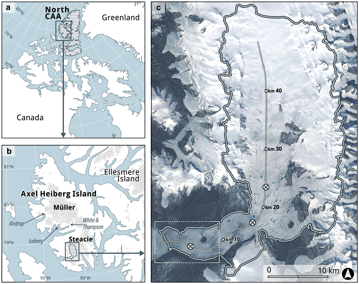
Out of 51 surge-type glaciers previously inventoried in the northern Canadian Arctic Archipelago (CAA: Ellesmere, Axel Heiberg, and Devon islands), the most dramatic terminus advances were documented on western Axel Heiberg Island, with three glaciers advancing between 4 and 7 km in the 1959–99 period (Copland and others, Reference Copland, Sharp and Dowdeswell2003). One of these, Good Friday Glacier (78° 33′N, 91° 30′W) is a ~50 km long marine-terminating outlet glacier of the Steacie Ice Cap on southern Axel Heiberg Island (Fig. 1). Good Friday Glacier (sometimes referred to as Good Friday Bay Glacier; henceforth GF) was first reported as actively surging in the 1950--60s (Müller, Reference Müller1969), and again in the 1990s (Copland and others, Reference Copland, Sharp and Dowdeswell2003). Recent observations indicate that the glacier terminus was still advancing in the 2000–15 period, with surface velocities reaching up to 350 m a−1 at the terminus (Van Wychen and others, Reference Van Wychen2014, Reference Van Wychen2016; Millan and others, Reference Millan, Mouginot and Rignot2017).
(a) Ice covered islands of the Northern Canadian Arctic Archipelago (horizontal hatch), Arctic Canada; (b) Good Friday Glacier (horizontal hatch), Axel Heiberg Island; (c) Good Friday Glacier. Base Image: Landsat 8, RGB composite, 7 July 2016. The black and white outline in (c) indicates the drainage basin, and the line corresponds to the glacier centreline. The dashed box marks the terminus region and the extent of Figs 3–4. The 3 round markers on the ice surface indicate the locations of 3 dual frequency GPS stations installed in 2015.
Overall there is a high spatial and temporal variability in glacier dynamics in the CAA, with most land-terminating glaciers gradually retreating and slowing over the past few decades in response to a sustained negative mass-balance regime (Heid and Kääb, Reference Heid and Kääb2012b; Schaffer and others, Reference Schaffer, Copland and Zdanowicz2017; Strozzi and others, Reference Strozzi, Paul, Wiesmann, Schellenberger and Kääb2017; Thomson and Copland, Reference Thomson and Copland2017). A few of the large marine-terminating glaciers have been shown to exhibit large interannual velocity variations, sometimes varying by >50 m a−1 between years, accompanied by changes in their terminus position and ice thickness (Van Wychen and others, Reference Van Wychen2014, Reference Van Wychen2016). While marked variations in flow rates have traditionally been attributed to surging behaviour, more recent studies suggest that not all flow variability observed in the CAA fits the classic definition of surging. Some instabilities in ice motion rather resemble short-lived pulse events, often restricted to the lower ablation area of glaciers, which may be related to tidewater glacier dynamics or basal topography (Van Wychen and others, Reference Van Wychen2014, Reference Van Wychen2016).
While previous studies indicate that the terminus of GF advanced by ~7.7 km between 1952 and 1999 (Müller, Reference Müller1969; Copland and others, Reference Copland, Sharp and Dowdeswell2003), the length and characteristics of the total advance remain poorly constrained due to limited observations between studies and lack of detailed knowledge of ice velocities. In this study, we reconstruct the evolution of GF from previous reports and a >50-year record of remotely sensed data. Combining observations of ice surface velocities, changes in terminus position, and ice surface and basal topography, we assess whether the glacier has undergone a continuous advance over the past seven decades and whether the observed changes can be explained by surging or another mechanism.
2. STUDY SITE
Axel Heiberg Island, in the northern CAA (Fig. 1), contains >1100 glaciers covering a total area of ~11,700 km2 and supports two major ice caps – the Müller and Steacie ice caps (Ommanney, Reference Ommanney1969; Thomson and others, Reference Thomson, Osinski and Ommanney2011). Ice surface velocities in the CAA typically range between <10 m a−1 in the interior of ice caps, increase to 30–90 m a−1 along the main trunks of tidewater glaciers and peak at 200–400 m a−1 at their termini. Typical values for land-terminating glaciers in the Canadian Arctic range between 20 and 50 m a−1 (Van Wychen and others, Reference Van Wychen2014).
Müller (Reference Müller1969) reported that, in the late 1940s and early 1950s, GF was land-terminating, and advancing behind a >1 km wide push moraine, at a steady rate of 20 m a−1, similar to other large glaciers in the region (e.g. Thompson Glacier). During the 1952–59 period, the rate of terminus advance rose to ~100 m a−1, and the lowermost 2 km of the glacier thickened and became crevassed. In the mid-1960s, the terminus advance reached a maximum of 200 m a−1, and ice motion increased to >250 m a−1 (Müller, Reference Müller1969). This was accompanied by a large increase in the number of crevasses and a chaotically broken-up surface. About 4–6 km up-glacier a rim of ice along the valley walls, 10–15 m above the glacier surface, suggested surface lowering. By the late 1960s the rate of terminus advance had decreased significantly (to ~100 m a−1). In the 17 years between 1952 and 1969, the terminus advanced ~2 km, ‘overriding’ most of the push moraine (Müller, Reference Müller1969).
By 1999 the ice front of GF had advanced an additional ~5.6 km (Copland and others, Reference Copland, Sharp and Dowdeswell2003). Copland and others (Reference Copland, Sharp and Dowdeswell2003) used this evidence, together with a heavily crevassed terminus and looped surface moraines, to classify the glacier as ‘confirmed surging’ with an active phase of at least 10 years and perhaps >40 years. By 2015 GF had advanced an additional ~2 km and continued to exhibit relatively high flow rates (>100 m a−1) over the entire length of the main trunk (Van Wychen and others, Reference Van Wychen2016).
3. METHODS
3.1. Ice extent
Near-annual changes in terminus position were mapped for 1972–2018 from optical satellite imagery, namely Landsat 1–8 and ASTER Level 1 products (Table 1), accessed through the US Geological Survey EarthExplorer data portal (http://earthexplorer.usgs.gov). These data products are geometrically/radiometrically corrected and accurately orthorectified, and therefore required no pre-processing. The terminus region was manually outlined in QGIS2.18 (QGIS Development Team, 2017) based on a total of 43 cloud-free images, preferentially acquired at the end of summer for minimal snow cover. No cloud-free images were available for 1994–97, resulting in a 4-year data gap. Outlining was performed at single pixel precision on false colour composites, while maintaining a constant scale to minimise errors due to changes in appearance between various spatial resolutions (15 m for ASTER; 30 m for Landsat TM, ETM+ and OLI; 60 m for Landsat MSS). Errors for manual delineation are generally within one pixel and accuracy tends to increase with image resolution and glacier size (Paul and others, Reference Paul2013). Errors in ice extent were assessed by repeated delineation performed on two Landsat scenes, at different resolutions (60 m in 1972; 30 m in 2018). Each terminus was outlined five times, and the relative area difference varied between 1.14 and 0.36% for the 60 and 30 m resolution images, respectively. The 1959 terminus position was mapped from a 1:60,000 scale aerial photograph obtained from the National Air Photo Library, Ottawa, Canada, based on an original survey flown by the Royal Canadian Air Force (RCAF) at an altitude of ~9000 m (Table 1). The air photo was manually coregistered to a base image (Landsat 8, 18 August 2017) using tiepoints. To better account for an irregular terminus geometry, and fluctuations in centreline position over the last six decades, area change in the terminus region was calculated from a fixed reference line (Fig. 2b) ~10 km up-glacier from the present-day ice front.
(a) Area change across the terminus region for 1959–2018. The blue vertical dotted line indicates the time when the terminus reached tidewater in 2006 and began calving. (b) Evolution of the terminus region over the study period, with terminus positions mapped at yearly (thin white lines), and decadal (thick white lines) intervals. Area change for all years was calculated from the dashed reference line at the right edge of the map. Base image: Landsat 8, 29 July 2017.

Imagery used for mapping terminus position. Sensor designations: Multispectral Scanner (MSS), Thematic Mapper (TM), Enhanced Thematic Mapper Plus (ETM+), Advanced Spaceborne Thermal Emission and Reflection Radiometer (ASTER), Operational Land Imager (OLI)

3.2. Ice velocities
3.2.1. Speckle tracking
Glacier surface velocities for 2006–18 were determined from speckle tracking on pairs of RADARSAT-1/2 images acquired on repeat 24-day orbits (Table 2). RADARSAT-1 imagery was obtained from the Geological Survey of Canada, and RADARSAT-2 through Natural Resources Canada and the Canadian Space Agency. Speckle tracking utilises a cross-correlation algorithm on coregistered pairs of synthetic aperture radar (SAR) images to determine surface ice displacement. We utilise a specially developed MATLAB offset and speckle tracking algorithm that has been extensively utilised for measuring glacier velocities in the Canadian Arctic (e.g. Short and Gray, Reference Short and Gray2005; Van Wychen and others, Reference Van Wychen2014, Reference Van Wychen2016), and has been shown to provide comparable results to those determined by commercial software packages (e.g. GAMMA InSAR) (Schellenberger and others, Reference Schellenberger, Van Wychen, Copland, Kääb and Gray2016). Image pairs were initially coregistered either manually (RADARSAT-1), or by calculating offsets from orbital parameters (RADARSAT-2). Displacements resulting from speckle tracking were then calibrated over stationary bedrock features to remove any systematic errors. Manual inspection of the data was undertaken to filter out erroneous displacements that arise from mismatching errors during the cross-correlation process. Final ice surface velocities were then interpolated from the filtered point displacements to a 100 m resolution raster dataset using an inverse distance weighting algorithm. Full details of the speckle tracking method are provided in Van Wychen and others (Reference Van Wychen2014, Reference Van Wychen2016). The method is most reliable when the ice surface remains relatively unchanged (i.e. little or no melt/snowfall) between images which, for northern CAA, restricts image acquisitions to mid-to-late winter (typically January--April). The velocities derived from speckle tracking therefore reflect ‘winter’ velocities, and should be regarded as annual minima as they omit any seasonal speedup events associated with enhanced summer melt.
Image pairs used for offset tracking

3.2.2. Feature tracking
Additional velocities were derived from feature tracking on pairs of annually separated, cloud-free optical satellite images from Landsat TM (1987/88, 1991/92) and ETM+ (1999/2000, 2010/11) (Table 2). As the method requires distinct surface features, summer images acquired in June--August were selected to ensure minimal snow cover. To enhance contrast between features, and therefore improve edge detection, a two-step filtering method was applied using the ‘raster’ package (Hijmans, Reference Hijmans2017) in R 3.4.3 (R Core Team, 2017). We used a 3 × 3 pixel kernel, corresponding to ~100 m on the 30 m resolution TM (band 3) images, and ~50 m on the 15 m resolution ETM+ (panchromatic band 8) scenes. Images were first smoothed (lowpass filtered) to reduce high-frequency noise, and then sharpened (highpass filtered) to attenuate low frequencies and enhance intensity contrasts between edges of small-scale surface features, mainly crevasses and melt channels, as well as large-scale longitudinal foliations. Displacements between images due to ice flow were tracked using a normalised cross-correlation algorithm implemented in the image correlation software CIAS (Kääb and Vollmer, Reference Kääb and Vollmer2000; Heid and Kääb, Reference Heid and Kääb2012a). The resulting displacement vectors were filtered, in both direction and magnitude, by applying a median filter on a ~500 m radius moving window using the ‘raster’ package (Hijmans, Reference Hijmans2017). Incorrect matches deviating by more than 45° in direction, and ±25% in magnitude, from the median of the neighbouring vectors were removed from the dataset. Final velocities were interpolated to a 100 m resolution raster using an inverse distance weighting algorithm and the ‘gstat’ package (Gräler and others, Reference Gräler, Pebesma and Heuvelink2016) in R (R Core Team, 2017).
3.2.3. Error analysis
The accuracy of both offset tracking methods was assessed from apparent displacements measured over stable terrain adjacent to the glacier. The average errors and standard deviation for feature tracking results were 19 ± 40 m a−1, or 9 ± 6 m a−1 after filtering erroneous matches. These values compare well with error margins of ~5–15 m a−1 determined here and in previous studies using the speckle tracking method in the CAA (e.g. Short and Gray, Reference Short and Gray2005; Van Wychen and others, Reference Van Wychen2014, Reference Van Wychen2016). Velocity results derived from speckle and feature tracking methods were also compared with field measurements from three dual frequency GPS (dGPS) stations mounted on poles drilled into the glacier surface 5, 16, and 23 km from the terminus (Fig. 1c). The stations recorded positions at 15 second intervals for an hour at midday each day, providing mean daily positions between July 2015 and July 2017. The difference in annual displacements derived from speckle tracking and dGPS observations from two overlapping 24-day periods in the winters of 2016 and 2017 is 3–5% (3–5 m a−1). These ‘winter’ velocities are 6–10% lower than annual velocities derived from the mean daily dGPS observations, which include periods of high velocity fluctuations over spring/summer months. In comparison, feature tracking results from two pairs of annually separated Landsat OLI images (2015/16, 2016/17) are within 0–12% (0–16 m a−1, ~9 m a−1 on average) of dGPS measurements collected over the same period.
3.3. Ice surface and bed elevation
Ice surface topography was extracted from the ArcticDEM (Porter and others, Reference Porter2018), produced by the Polar Geospatial Centre from DigitalGlobe (Worldview-1/2/3 satellites) imagery. The DEM was generated from overlapping stereo pairs of optical images at ~0.5 m resolution acquired between 2012 and 2015, and processed into 5 m resolution mosaics in 50 x 50 km tiles (https://www.pgc.umn.edu/data/arcticdem/). The reported horizontal and vertical accuracy of the final product is within 0.2 m of the ice surface at the time of image acquisition (Noh and Howat, Reference Noh and Howat2015), and the mean vertical residual after correction with clusters of IceSAT altimetry data was −0.002 m and 0.015 m for tile 32_31, and 0.003 m for tile 32_32.
We use bed elevation data from airborne radar measurements from the Centre for Remote Sensing of Ice Sheets (CReSIS) Multichannel Coherent Data Depth Sounder (MCoRDS) operating at a frequency range of 180–210 MHz (Allen, Reference Allen2013). The radar was flown at an altitude of 500–900 m above the ice surface along the full length of GF in March 2014 as part of NASA's Operation IceBridge. The data were gridded using radar tomography processing into a ~3 km wide swath, with an along-track sample spacing of 16 m, and a cross-track spacing of ~30 m at nadir and ~100 m at the edge of the swath. The final product is a 25 m resolution map of basal topography (CReSIS, 2016). Tomography requires good signal to noise ratio to accurately differentiate between off-nadir echoes. Vertical accuracy therefore varies with surface roughness, and englacial/basal water content. Studies have found the uncertainty in ice thickness to be within 10–20 m (Paden and others, Reference Paden, Akins, Dunson, Allen and Gogineni2010; Wu and others, Reference Wu2011; Jezek and others, Reference Jezek, Wu, Paden and Leuschen2013).
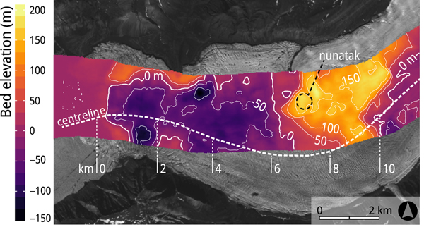
Both bed and surface elevation profiles were extracted along the centreline of the glacier, with the exception of a ~3 km long segment ~6 km from the terminus where the IceBridge flightline deviated from the centreline and passed over a large nunatak (Fig. 3). Over this region, the bed topography was extracted from the edge of the swath, with the furthest extrapolated point being ~170 m north of the centreline.
Bed elevation map from IceBridge MCoRDS tomography data. The flightline deviates from the glacier centreline 5–8 km from the terminus. Contours at 50 m intervals.

4. RESULTS
4.1. Terminus position
Results show a terminus advance of 8.6 km along the centreline of GF over the 1959–2018 period (Fig. 2), amounting to ~9.3 km since the first observations in 1948. The area of the terminus region increased at a steady rate of ~1 km2 a−1 throughout the 1970–80s, slowed by 25% (to 0.73 km2 a−1) in the 1990s, and dropped dramatically, by an additional 82% (to 0.18 km2 a−1) since ~2006–08. The terminus increased in area by ~39 km2 over the last 59 years (Fig. 2), representing a ~5% increase in glacier area compared to a total basin size of 800 km2.
The 1959 air photo shows the ice front being channelled south of the nunatak (Fig. 4a), ~7 km from the current terminus position. This nunatak is the surface expression of a >150 m high ridge extending approximately north to south across the glacier channel (Fig. 3). In 1959, two small looped moraines were visible along the southern margin, one immediately at the terminus (Fig. 4a), and the other ~4 km up-glacier. Where the ice is channelled into the narrow trough south of the nunatak, the lowermost 2 km of the terminus was broken up by a field of transverse crevasses extending across the front in an arcuate pattern (concave down-glacier). In comparison, the surface of the northern half of the terminus was relatively smooth and showed some splaying crevasses in the along-flow direction. The more advanced southern half was separated from fjord waters by a partially submerged 800 m wide push moraine. Müller (Reference Müller1969) reported that by 1969 the terminus had overridden most of this moraine. At the time of the first Landsat image in 1972, GF had become marine-terminating and continued to be so throughout the remainder of the 1970s (Figs 4b and 5a). However, at the beginning of the 1980s a new moraine had started to emerge at the terminus and by 2000, the ice front was once again separated from fjord waters by a ~600 m wide moraine (Fig. 4c).
Evolution of the terminus over the study period (a) RCAF air photo, 29 June 1959; (b) Landsat 2, 20 August 1977; (c) Landsat 7, 20 June 2000; (d) Landsat 7, 27 July 2006; (e) Landsat 8, 14 August 2017.

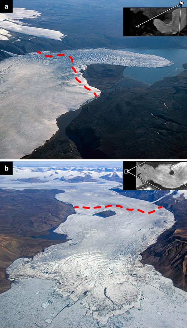
Terminus of Good Friday Glacier on (a) 24 August 1977 (looking southwest), and (b) 1 July 2008 (looking east), with the splayed lobe advancing into the sea ice. The red outlines approximate the 1959 terminus position. The two insets indicate the direction from which the photos were taken, with white lines representing the camera viewshed. Photos: Jürg Alean (http://www.swisseduc.ch).

The terminus continued to advance behind the moraine until 2006–08. Throughout this period the surface at the glacier front remained relatively smooth with some splaying crevasses forming right along the terminus. As the ice overrode the frontal moraine between 2006 and 2008 (Fig. 4d), the terminal zone of the ice tongue became broken up by a field of transverse crevasses extending ~1 km up-glacier (Fig. 4e). From that point on, fluctuations in terminus position become highly seasonal – each winter the ice front pushes forward, splaying out into the sea ice in a large digitate lobe (Fig. 5b), and disintegrates within a few days as the sea ice clears the fjord the following summer. The southern portion of the terminus has therefore become essentially stationary at approximately the position where the terminal moraine was last seen in 2006. Meanwhile, over the last decade, the northern sector of the front has advanced into the fjord by ~1.5 km, although its rate of advance has declined considerably in the last 3 years (Fig. 2).
4.2. Velocity patterns
Results show a general decrease in surface velocities over the full length of the glacier since the late 1980s (Fig. 6b). The glacier bed first drops below sea level around km 20 (Fig. 6a), approximately where it changes flow direction (from southerly to south-westerly), however, this is not continuous over the full width of the channel and most of the ice remains grounded above sea level. Ice motion shows higher spatial variability down-glacier from this point, with a major velocity peak immediately down-glacier of the 150 m high (>50% of ice thickness) ridge extending across the glacier channel at km 9 (Fig. 3). The ArcticDEM surface profile (Fig. 6a) shows a thickening up-glacier from this topographic high, and a marked steepening and 70 m elevation drop immediately down-glacier from it. Flow rates at this location dropped from 470 m a−1 in the late 1980s, to 170 m a−1 in 2018, but have consistently remained 30–50% higher than on either side of the bump (Fig. 6). Downstream of the ridge, the ice is grounded in an overdeepening which drops to 50–70 m below sea level. The bed slope is reversed over the lowermost 1.5 km (Figs 3 and 6a).
(a) Ice surface (blue; ArcticDEM) and bed elevation (black; Icebridge MCoRDS) profiles. (b) Centreline ice surface velocities for 1987–2018. Profiles spanning two consecutive years (e.g. 87/88) correspond to velocities extracted from feature tracking. Those spanning a single year were derived from speckle tracking. The yellow diamond indicates velocities recorded at the terminus in 1959.

In the 1980–90s velocities decreased towards the ice front, as is typical for land-terminating glaciers (Van Wychen and others, Reference Van Wychen2016), but starting in 2006 the pattern changed and flow rates now rapidly increased over the lowermost ~4 km. Velocity profiles for 2006–18 show velocities ranging between 100 and 250 m a−1 along the main trunk of the glacier, and reaching >350 m a−1 at the terminus. These values are comparable to those recorded in the 1960s (~250 m a−1) in the terminus region (presently km 8) when Müller (Reference Müller1969) suggested that the glacier was actively surging. Despite continued fast flow, and consistently high velocities at the terminus, the glacier has slowed by ~50–100 m a−1 over much of its length over the last decade (Fig. 6b).
5. DISCUSSION
Good Friday Glacier is located within a region where mass balance has been dominated by a trend of accelerating mass loss (e.g. Gardner and others, Reference Gardner2011, Reference Gardner2013; Sharp and others, Reference Sharp2011; Lenaerts and others, Reference Lenaerts2013; Noël and others, Reference Noël2018). The uninterrupted advance of the terminus since 1948, and the relatively high (>100 m a−1) velocities recorded along the full length of the glacier (Figs 6b and 7), are therefore unexpected. This raises the question as to what mechanism(s) has been driving this asynchronous behaviour. We evaluate two factors, namely mass balance and dynamic instabilities, as potential causes for the long-term advance. Then, we examine the spatial variability in dynamics in the terminus region of GF in relation to local variations in bedrock topography, and propose an alternate interpretation to surging for the temporal evolution of ice motion at the glacier front throughout the advance.
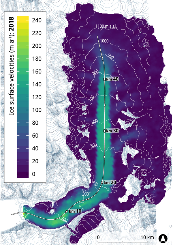
Ice surface velocities along Good Friday Glacier, derived from speckle tracking of RADARSAT-2 image pairs from 2 and 26 January 2018. Longitudinal velocity profiles were extracted along the centreline (black and white line). A ~150 m high ridge runs southeast from the nunatak, roughly following the 200 m contour 9 km from the terminus.

5.1. Mass balance
Annual mass-balance estimates for the northern CAA have been mostly negative since the early 1960s (Koerner, Reference Koerner2005), and recent studies indicate accelerated mass loss in the last two decades (Gardner and others, Reference Gardner2011; Lenaerts and others, Reference Lenaerts2013; Millan and others, Reference Millan, Mouginot and Rignot2017; Box and others, Reference Box2018; Noël and others, Reference Noël2018). Using a regional climate model Noël and others (Reference Noël2018) showed that, for the 1958–95 period, glaciers and ice caps in the northern CAA experienced an overall negative mass budget with losses totalling 11.9 ± 11.5 Gt a−1. Since the mid-1990s, losses more than doubled, reaching 28.2 ± 11.5 Gt a−1 (Noël and others, Reference Noël2018). This sharp increase in mass loss has been in direct response to rising summer air temperatures, resulting in higher surface melt rates and longer melt seasons (Gardner and others, Reference Gardner2011; Sharp and others, Reference Sharp2011; Mortimer and others, Reference Mortimer, Sharp and Wouters2016, Reference Mortimer, Sharp and Van Wychen2018; Noël and others, Reference Noël2018). As a result of this sustained negative mass-balance regime, most land-terminating glaciers in the CAA have been retreating and slowing down (Thomson and others, Reference Thomson, Osinski and Ommanney2011; Heid and Kääb, Reference Heid and Kääb2012b; Schaffer and others, Reference Schaffer, Copland and Zdanowicz2017; Thomson and Copland, Reference Thomson and Copland2017).
An inventory of glacier change on Axel Heiberg Island from 1959 to 2000 showed a dominant trend of glacier retreat, with greatest mass loss on small independent glaciers, including the loss of 90% of ice masses smaller than 0.2 km2 (Thomson and others, Reference Thomson, Osinski and Ommanney2011). However, these losses were partially offset by glacier advances in basins dominated by outlets from the Müller and Steacie ice caps. Three of them (GF, Iceberg and Airdrop glaciers) were classified as surge-type (Copland and others, Reference Copland, Sharp and Dowdeswell2003), and their advances were therefore attributed to surge activity. In general, the advancing glaciers were found to be larger on average (Thomson and others, Reference Thomson, Osinski and Ommanney2011). Modelling studies have shown that large Arctic glaciers with shallow surface slopes generally have longer response times than smaller ice masses in the region, and therefore require centuries longer to adjust to changes in surface mass balance following a change in climatic conditions (Raper and Braithwaite, Reference Raper and Braithwaite2009). A comparison of in situ velocity measurements from the 1960 to 1970s and 2012–16 on White Glacier, a ~14 km long mountain glacier located ~65 km N of upper GF, shows a general long-term decrease in flow rates, especially towards the glacier terminus (Thomson and Copland, Reference Thomson and Copland2017). While White Glacier retreated ~250 m between 1948 and 1995, the neighbouring Thompson Glacier, a land-terminating outlet of the Müller Ice Cap, advanced by ~950 m over the same period (Cogley and Adams, Reference Cogley and Adams2000; Thomson and others, Reference Thomson, Osinski and Ommanney2011), and only started retreating at some time in the 2000s (Cogley and others, Reference Cogley, Adams and Ecclestone2011). One possible explanation for this contrasting behaviour may be related to the different geometries of White vs. Thompson glaciers and the difference in their respective response times. Considering the significantly larger size of the Thompson (~390 km2) compared to White Glacier (40 km2), the longer advance may therefore reflect a delayed response to a positive mass-balance regime in the cooler conditions of the Little Ice Age (Cogley and Adams, Reference Cogley and Adams2000; Cogley and others, Reference Cogley, Adams and Ecclestone2011).
In comparison, GF is the largest of the three glaciers (800 km2), and has been advancing continuously to this day. However, our results show that surface velocities have decreased by ~50–100 m a−1 over much of the glacier length over the last decade, and ice motion in the terminus region has been slowing since at least the late 1980s. Although the uninterrupted advance over the last seven decades could be related to positive mass-balance conditions of the Little Ice Age, the gradual slowdown supports the idea that the glacier has been losing mass similarly to other glaciers in the region. Indeed, Noël and others (Reference Noël2018) showed that the average surface mass balance of GF has been negative over much of its length over the 1958–2015 period. Alternatively, the asynchronous behaviour of both GF, and until recently the Thompson, may instead be related to a dynamic instability, such as surging (Copland and others, Reference Copland, Sharp and Dowdeswell2003).
5.2. Dynamic instabilities
5.2.1. Glacier surging
Dynamic instabilities typically occur when short-term flow rates deviate (significantly) from long-term balance velocities. In these cases, glaciers fail to maintain a steady-state profile and instead experience changes in geometry while cycling between fast and slow flow regimes. On surge-type glaciers, velocity fluctuations occur in response to changes in driving stress, which typically increases along with thickening and surface steepening during quiescence, eventually initiating the surge (Raymond, Reference Raymond1987). The classic pattern of surging involves a down-glacier propagation of a surge front, resulting in dramatic velocity increases over most of the glacier length, rapid terminus advance and significant surface lowering. The resulting dynamic thinning eventually reduces the driving stress, allowing the glacier to slow down thus leading to surge termination. The quiescent phase typically coincides with terminus retreat (Meier and Post, Reference Meier and Post1969; Raymond, Reference Raymond1987).
Although glacier surges are not typically thought of as a direct response to climate, external climatic factors dictate changes in mass balance, which in turn influence the length and intensity of surges (Eisen and others, Reference Eisen, Harrison and Raymond2001; Copland and others, Reference Copland2011). Surge-type glaciers in high accumulation regions with temperate thermal regimes (e.g. Alaska, Yukon) typically have a much shorter active phase (1–2 years) than those in polar environments with limited snowfall and polythermal regimes such as Svalbard (Dowdeswell and others, Reference Dowdeswell, Hamilton and Hagen1991; Murray and others, Reference Murray, Strozzi, Luckman, Jiskoot and Christakos2003) and the Canadian Arctic (Copland and others, Reference Copland, Sharp and Dowdeswell2003; Short and Gray, Reference Short and Gray2005). On Svalbard, the surge phase generally lasts 3–10 years, and surge termination is a gradual process which can take several years (Dowdeswell and others, Reference Dowdeswell, Hamilton and Hagen1991). Previous observations of surging glaciers in the northern CAA suggest that the surge phase may last anywhere from 5 to 10 years, to as much as 50 years (Hattersley-Smith, Reference Hattersley-Smith1969; Müller, Reference Müller1969; Copland and others, Reference Copland, Sharp and Dowdeswell2003; Short and Gray, Reference Short and Gray2005; Van Wychen and others, Reference Van Wychen2016).
One issue with long surge cycles is the difficulty in identifying the period of surge initiation and termination, and therefore accurately constraining the duration of the active phase. This is partly due to the limited timespan covered by many datasets, and the generally lower velocities and more gradual changes associated with surging in polar environments. This introduces an observational bias, and few polar glaciers have been observed to surge more than once. Surge-type glaciers can be identified by the presence of features indicative of flow instabilities. Looped moraines and ice foliations on the glacier surface are diagnostic of oscillatory behaviour and are therefore generally regarded as reliable signs of surging (Meier and Post, Reference Meier and Post1969; Clarke, Reference Clarke1987; Copland and others, Reference Copland, Sharp and Dowdeswell2003). Previous studies have identified 13 glaciers with signs of unstable flow on Axel Heiberg Island. Most of these were classified as likely or possibly surge-type, mainly based on the presence of said surface features. Of the 13 glaciers, the largest three (GF, Iceberg, Airdrop) experienced fast flow and important terminus advances (4.5–7 km) in the 1959–99 period, and were thus confirmed as surge-type (Copland and others, Reference Copland, Sharp and Dowdeswell2003). While all three have decelerated since 1999, Iceberg Glacier is the only one to have displayed a cyclic behaviour that is typical for surging glaciers (Van Wychen and others, Reference Van Wychen2016).
Iceberg Glacier is a large (~750 km2) marine-terminating outlet glacier which drains the western side of Müller Ice Cap, located ~70 km NNW of the upper parts of GF. In 1959, the terminus was retreating (Ommanney, Reference Ommanney1969) and the ice surface was heavily potholed over an extensive area, two characteristics of stagnating glaciers in the quiescent phase of the surge cycle. By 1999, the glacier had advanced ~5 km (Copland and others, Reference Copland, Sharp and Dowdeswell2003). Following studies reported high flow rates over the entire trunk of the glacier (Short and Gray, Reference Short and Gray2005; Van Wychen and others, Reference Van Wychen2016), reaching up to ~575 m a−1 at the terminus in the 1990s (Copland and others, Reference Copland, Sharp and Dowdeswell2003). This was followed by a period of terminus retreat coinciding with slowdown, which reportedly began at the terminus in the early 2000s, and had propagated over the entire trunk by ~2010. Iceberg Glacier has been essentially stagnant since, and the terminus retreated ~1.5–2.5 km over the 2000–14 period (Van Wychen and others, Reference Van Wychen2016). This is the only glacier on Axel Heiberg Island to have been observed in the quiescent phase of the surge cycle twice, with the evidence pointing to an active phase lasting between 10 and 30 years.
Iceberg Glacier and GF are the largest, and only two marine-terminating glaciers on the island. Although they are similar in their general configuration and climatic setting, the cyclic oscillations in ice motion observed on Iceberg Glacier indicate that its dynamics are at least partly decoupled from the long-term climate trend of negative mass balance since 1958 (Noël and others, Reference Noël2018). This contrasts with the evidence from GF where no retreat has yet been recorded, and there are no observations of the glacier in the quiescent phase of the surge cycle. The initial speedup in the 1950s may correspond to surge initiation, and the gradual decrease in ice motion and terminus advance of the last decade may in turn indicate that the glacier is now approaching quiescence. If GF is indeed surging, the sustained terminus advance of the last 70 years would correspond to the longest active phase ever recorded, both on a regional and global scale.
5.2.2. A spectrum of flow instabilities
Müller (Reference Müller1969) concluded that while GF exhibited some tell-tale signs of surging, including an increase in surface velocities an order of magnitude above background levels, intense surface crevassing and a marked terminus advance, he found no clear sign of a surge front propagating down-glacier. Additionally, the long active phase (>10 years) and the lack of evidence of previous surges distinguished it from other classic examples of surging (Meier and Post, Reference Meier and Post1969). As evidenced by Iceberg Glacier and other glaciers in the CAA, 10 years may not be particularly long for an active surge phase in polar environments, but 70 years is significantly longer than any surge reported to date.
With longer surge cycles, evidence of past surge activity becomes less evident. The heavily folded longitudinal foliations and the two small looped moraines visible near the terminus of GF on the 1959 air photo (Fig. 4a) may indeed be interpreted as signs of unstable flow, but do not in themselves provide evidence of past surges. The moraines may have instead formed as GF advanced into previously unglaciated terrain, entraining the snouts of slower glaciers which, until then, had been flowing unhindered onto the main valley floor below. On the other hand, the absence of characteristic surge features does not mean that a given glacier has not surged in the past. Similarly, the lack of evidence of a clear surge front propagating down-glacier does not exclude the possibility that the changes in glacier geometry occurring on GF in the 1950s may correspond to a phase of surge initiation. The thickening at the terminus, the rapid advance, and thinning further up-glacier may indicate fast flow conditions initiating at the terminus, and propagating up-glacier instead. This behaviour has been observed on several marine-terminating glaciers on Svalbard (e.g. Murray and others, Reference Murray, Strozzi, Luckman, Jiskoot and Christakos2003; Sevestre and others, Reference Sevestre2018), as well as in the Canadian Arctic (Van Wychen and others, Reference Van Wychen2016), but is rather unlikely to have occurred on GF at the time since the terminus was then grounded well above sea level, behind a ~1 km wide and 30 m high moraine (Müller, Reference Müller1969). That being said, it would appear that the ice front reached fjord waters at some time in the mid-1960s, and the terminal moraine became progressively submerged as the terminus advanced past the nunatak and into a wider section of the valley (Fig. 4). This approximately coincides with the area where the bed dips below sea level 6–7 kms upglacier from the current terminus (Fig. 6a). Tidewater dynamics may have therefore played a role in encouraging fast flow in the mid-1960s, and/or contributed to the brief drop in the rate of terminus advance at the end of that decade.
Although several factors suggest a dynamic instability, there is no unequivocal evidence of surging behaviour in the classic sense of the term. However, it is well established that dynamic instabilities encompass a wide spectrum of behaviours, with the duration, initiation, propagation and termination of fast flow events varying between glaciers and regions. Glaciers can therefore experience significant interannual variations in ice motion without necessarily being classified as surge-type. Studies describe cases of partial surges, or pulse-like events, which broadly encompass all periodic episodes of unstable flow resulting in more moderate changes than those usually associated with surging (Raymond, Reference Raymond1987; Turrin and others, Reference Turrin, Forster, Sauber, Hall and Bruhn2014; Van Wychen and others, Reference Van Wychen2016). Van Wychen and others (Reference Van Wychen2016) differentiated surging from pulsing by the velocity structure and pattern of initiation and propagation of fast flow conditions in CAA glaciers. They identified several marine-terminating glaciers as pulse-type, as fast flow initiated at the terminus and remained restricted to their lowermost reaches where the bed is grounded below sea level.
The dynamics of large tidewater glaciers are generally more variable than for land-terminating ones, as ice motion is controlled by a series of additional factors related to the force balance at the ice/ocean interface (e.g. Pfeffer, Reference Pfeffer2007; Nick and others, Reference Nick, Vieli, Howat and Joughin2009; Straneo and others, Reference Straneo2013). Marine-terminating glaciers are known to undergo asymmetric cycles of slow advance followed by rapid retreat and terminus disintegration through calving. The tidewater glacier cycle underlines the importance of glacier-specific factors, such as basal topography, in driving unstable flow behaviour (Meier and Post, Reference Meier and Post1987; Alley, Reference Alley1991; Brinkerhoff and others, Reference Brinkerhoff, Truffer and Aschwanden2017). The key point is that the distinction between surging and other unstable flow behaviour is not clear cut, and in many cases it is a question of semantics. This underlines the importance of considering the periodic oscillations attributed to surging as part of a wider spectrum of dynamic instabilities (Raymond, Reference Raymond1987; Turrin and others, Reference Turrin, Forster, Sauber, Hall and Bruhn2014; Van Wychen and others, Reference Van Wychen2016), including single episodes of fast flow and short-lived or localised speedup events.
5.3. Perturbations in bedrock topography
The idea that GF is (or was) surging mainly depends on how one interprets the changes in ice motion occurring at the glacier terminus in the 1950–60s. It is therefore useful to review the evidence for fast flow, and examine alternate mechanisms as potential triggers. The way in which present-day ice velocity and glacier geometry patterns vary can provide insight into the evolution of ice motion at the terminus as it advanced into previously unglaciated terrain. On a local scale, variations in surface geometry and ice motion depend on basal conditions (bedrock topography and basal water pressure), which modulate resistance to flow through along-flow gradients in basal and lateral drag (Cuffey and Paterson, Reference Cuffey and Paterson2010). Ice typically thickens through compression up-glacier from bedrock bumps, or where flow converges into narrow valley sections and thins through extension as it flows over the obstacle, or out of the constriction. Driving stress rises with increasing surface slope, which then leads to faster flow and increased crevassing over the bump or through the constriction (Gudmundsson, Reference Gudmundsson2003; Raymond and Gudmundsson, Reference Raymond and Gudmundsson2005; Sergienko, Reference Sergienko2012). Longitudinal stress gradients further modulate ice flow through differential pushes and pulls, such that where velocities increase along a flowline, the faster flowing ice is held back by slower ice further up-glacier, which is in turn entrained by the faster ice downstream. Through the propagation of longitudinal stresses, extensional flow in a region of low basal drag may therefore induce dynamic thinning and a velocity increase further up-glacier (Cuffey and Paterson, Reference Cuffey and Paterson2010). On the downstream side of an obstacle or constriction, the ice experiences longitudinal compression as it flows into slower moving ice, and consequently slows down (Sergienko, Reference Sergienko2012).
On GF, ice surface velocities increase in the vicinity of the nunatak, where ice flows over the topographic high extending across the glacier channel at km 9 (Fig. 6). Flow rates measured over that area reached ~250 m a−1 in the 1960s (Müller, Reference Müller1969), and have remained consistently high since the late 1980s, ranging between 160 and 470 m a−1 (Fig. 6). This localised velocity peak, and the variations in surface elevation, namely thicker ice on the up-glacier side of the bump, and steepening and surface drop down-glacier from it, are consistent with ice flow anomalies in response to an irregular bedrock topography (Gudmundsson, Reference Gudmundsson2003; Raymond and Gudmundsson, Reference Raymond and Gudmundsson2005; Sergienko, Reference Sergienko2012).
Müller (Reference Müller1969) observed a series of changes in ice motion in the 1950–60s, including (a) thickening at the ice front, (b) rapid frontal advance, (c) sudden speedup, and (d) increased crevassing. These occurred as the glacier front advanced over this bedrock bump, and into the narrow trough south of the nunatak. The initial thickening at the terminus may have been related to a combination of longitudinal compression on the upstream side of the 150 m high ridge, and lateral compression where the 5 km wide ice front was channelled into the 2 km wide constriction (Fig. 4). Thicker ice would have encouraged fast flow, longitudinal extension, and thinning further up-glacier. The sudden increase in the number of crevasses and the chaotically broken up surface were likely a result of longitudinal and lateral compression followed by longitudinal extension (Hudleston, Reference Hudleston2015). Similar intense crevassing has also been observed on surging glaciers following the passage of a surge front (Kamb and others, Reference Kamb1985; Lawson and others, Reference Lawson, Sharp and Hambrey1994; Murray and others, Reference Murray, Dowdeswell, Drewry and Frearson1998). Indeed, all these changes (a–d) can be associated with surging. It is therefore conceivable that, as the glacier reached the constriction south of the nunatak in the 1950s, the reported changes in ice motion may have been similar to those occurring during surge initiation. This was followed by a (brief) drop in the rate of terminus advance in the second half of the 1960s, which may have been related to a change in the force balance at the ice front as the glacier reached sea level. While the ice was grounded below sea level, the terminus was separated from fjord waters by the push moraine, which would have prevented calving.
Flow rates tend to increase towards the termini of tidewater glaciers and areas grounded below sea level as effective pressure, and therefore basal drag, both drop where the glacier approaches floatation (Benn and others, Reference Benn, Warren and Mottram2007). Lateral drag, on the other hand, is inversely proportional to trough width, and higher velocities occur where the fjord widens and flowlines diverge (Benn and others, Reference Benn, Warren and Mottram2007). Fjord narrowings and topographic highs both act as pinning points which can stabilise the glacier margin, thus controlling the magnitude of advance and retreat (Benn and others, Reference Benn, Warren and Mottram2007; Gudmundsson and others, Reference Gudmundsson, Krug, Durand, Favier and Gagliardini2012; Jamieson and others, Reference Jamieson2012; Enderlin and others, Reference Enderlin, Howat and Vieli2013; Carr and others, Reference Carr2015). Rapid advance in the mid-1960s may have occurred in response to increased basal water pressure at the terminus where the bed drops below sea level, accompanied by a drop in lateral drag where the valley widens. The presence of weak and easily deformable marine sediments at the ice/bed interface may have further enhanced basal motion (Clarke, Reference Clarke1987). The slowdown at the end of the 1960s may at least in part be explained by a reduction in driving stress induced by dynamic thinning in response to extensional flow (Cuffey and Paterson, Reference Cuffey and Paterson2010).
At the beginning of the 1970s the glacier had advanced into a basal overdeepening dipping to 70 m below sea level (Fig. 6a), and the rate of terminus advance increased once again. It has been argued that the advance rate of tidewater termini is influenced by sedimentation at the grounding line and the presence of a terminal moraine shoal, which can act as a pinning point, reduce calving rates and stabilise the ice front (Meier and Post, Reference Meier and Post1987; Alley, Reference Alley1991; Brinkerhoff and others, Reference Brinkerhoff, Truffer and Aschwanden2017). The advance of the terminus into the basal overdeepening may have therefore been facilitated by the formation of a submarine sediment shoal at the grounding line. This shoal was subsequently thrust up above water level (Fig. 4c) by the advancing ice front where the bed slopes upward in the direction of flow between kms 2–4.
The velocity profile at the terminus for the 1980–90s was characteristic of land-terminating glaciers, with velocities decreasing towards the glacier front. Velocities for 2006–18 are markedly different, with an acceleration towards the glacier front, reflecting a pattern characteristic of marine-terminating glaciers (Fig. 6b). The moment when the front reached tidewater in 2006 also coincides with a change in the crevasse pattern in the terminal zone, from some longitudinal splaying crevasses to transverse crevassing (Fig. 4), suggesting a transition from a compressive to an extending flow regime (Colgan and others, Reference Colgan2016). The longitudinal crevasses likely formed in response to longitudinal compression and resistance to flow where the ice front advanced over an upward sloping bed. The transverse crevasses are in turn indicative of longitudinal extension and high flow rates in areas of reduced resistance to flow, such as where ice flows into deeper water and/or into a widening fjord (Hambrey and Lawson, Reference Hambrey and Lawson2000; Colgan and others, Reference Colgan2016).
Today GF is in a stable extended position, with the terminus grounded on the moraine shoal, at the head of a wider section of the fjord, and any advance is approximately balanced out by calving losses. Since the ice entered the fjord in 2006–08, the southern portion of the glacier front started experiencing a seasonal cycle of advance/retreat linked to the presence/absence of sea ice in the fjord. A number of studies have reported the role of sea ice and ice mélange in limiting calving in the winter (e.g. Amundson and others, Reference Amundson2010; Howat and others, Reference Howat, Box, Ahn, Herrington and McFadden2010; Walter and others, Reference Walter2012; Cassotto and others, Reference Cassotto, Fahnestock, Amundson, Truffer and Joughin2015; Krug and others, Reference Krug, Durand, Gagliardini and Weiss2015). Evidence shows that sea ice can essentially act as a thin ice tongue and provide enough backstress to stabilise the terminus and prevent calved icebergs from drifting away (Amundson and others, Reference Amundson2010). We observe this process in the winter as the terminus of GF advances several hundred meters into the sea ice, forming a wide digitate lobe of calved ice, or ice mélange (Fig. 5b). This transient terminus then disintegrates rapidly (within a few days) as the sea ice clears the fjord in the summer (usually late July, early August). Without the stabilising resistive force provided by the sea ice, the southern part of the ice front is forced to retreat to its last stable position, approximately where the moraine was last seen in 2006. The asymmetry between the rate of advance of the southern and northern sections of the glacier front suggests the presence of local variations in basal/lateral drag. Until recently, the continued advance of the northern section of the front may have been facilitated by the geometry of the shoreline. However, the advance has slowed significantly over the last few years as the ice moved past the pinning point where the fjord widens.
6. SUMMARY AND CONCLUSIONS
Based on previous reports extending back to 1948, observations of changes in terminus position since 1959, and ice surface velocities since the late 1980s, we have reconstructed the evolution of GF over the past seven decades. Our results show an uninterrupted terminus advance of ~ 9 km spanning the last 70 years, which is the longest advance ever observed for a Canadian glacier and contrasts with the dominant regional trend of accelerated mass loss and glacier retreat over the past century. If this advance is interpreted as a surge it would correspond to the longest active phase ever recorded globally. The initial thickening at the ice front, followed by rapid terminus advance, increase in surface crevassing and surface drawdown, are all features characteristic of a classic surge. The gradual slowdown of the last decade could then be interpreted as the glacier approaching the quiescent phase of the surge cycle. However, without evidence of prior fast flow events or any other periodic oscillations in ice motion, we cannot conclude that the present behaviour is cyclic in nature. Rather than the standard definition of a surge, driven by periodic changes in subglacial hydrology or basal thermal regime (Murray and others, Reference Murray, Strozzi, Luckman, Jiskoot and Christakos2003), an alternate explanation is that the glacier terminus underwent a single brief period of unstable advance associated with perturbations in bedrock topography.
The fact that velocity patterns remained spatially consistent throughout the study period underlines the role of bedrock features, including topographic highs and basal overdeepenings, in modulating ice motion. We suggest that what was interpreted as the start of a surge in the 1950s may have at least in part been initiated by the terminus advancing into previously unglaciated terrain in an area favourable to the development of fast flow conditions. The initial thickening observed by Müller (Reference Müller1969) was likely triggered by mass buildup due to downstream resistance to flow where flowlines converge over the bedrock bump south of the nunatak. Fast flow first developed over the ridge in the 1950s and was likely further encouraged once the terminus advanced into an overdeepening below sea level. The brief drop in the rate of terminus advance at the end of the 1960s, as well as the current position of the ice front at the mouth of the fjord, may both be related to the presence of basal and lateral pinning points which stabilise the terminus and therefore control the rate of frontal advance. This interpretation could explain the sudden and localised changes in ice dynamics at the ice front in the 1950–60s, although it fails to explain the continued advance over the last seven decades.
The uninterrupted advance and relatively high flow rates along the entire length of the glacier do not in themselves provide evidence of surging or other unstable flow behaviour. Without additional observations of ice surface velocities above the terminus region spanning the initiation of fast flow conditions in the 1950–60s, we are unable to confirm whether the sudden speedup was related to a dynamic instability involving the entire length of the glacier, or rather a localised response to perturbations in basal topography. However, if it were a temporary instability such as a surge or surge-like event, flow rates would have eventually dropped as a result of surface drawdown and the rapid transfer of mass towards the terminus. Additionally, the localised velocity peak remained a permanent feature, constrained over the bedrock bump, indicating continued mass input from up-glacier throughout the advance. In this perspective, it is somewhat analogous to flow through an icefall, where permanent fast flow develops as a result of stress buildup at the boundary between areas of high and low basal drag.
The key point is that the behaviour of GF was, and still is, out of sync with similar ice masses in the Canadian Arctic, and with current climatic conditions. At this point, there is no evidence to suggest that the large-scale mass flux of GF deviates from steady-state flow conditions, and more investigations are required to determine the role of long-term mass-balance trends in driving the ongoing advance. Whether the result of a dynamic instability, or a delayed response to past (positive) mass-balance conditions of the Little Ice Age, these observations confirm the fact that not all glaciers in the CAA respond in the same way to similar environmental forcings. Identifying the factors causing this variability in ice motion is required to improve understanding of how glacier dynamics might evolve in a changing climate.
ACKNOWLEDGMENTS
This work was supported by the Natural Sciences and Engineering Research Council of Canada, Fonds de Recherche du Québec – Nature et Technologies, Ontario Graduate Scholarship, ArcticNet, Polar Continental Shelf Program, Canada Foundation for Innovation, Ontario Research Fund and the University of Ottawa. We thank the Nunavut Research Institute and the communities of Grise Fiord and Resolute Bay for permission to work on Good Friday Glacier. We acknowledge the Canadian Space Agency and NASA for acquiring the MCoRDS ice penetrating radar data over the glacier. The tomography radar data products were generated by CReSIS (Center for Remote Sensing of Ice Sheets) with support from the University of Kansas, NASA Operation IceBridge grant NNX16AH54G, and NSF grant ACI-1443054. The ArcticDEM was created from DigitalGlobe, Inc., imagery and provided by the Polar Geospatial Center funded under National Science Foundation awards 1043681, 1559691 and 1542736.


 Open access