Introduction

Satellite altimeter measurements of ice-sheet elevation began in 1975 with the launch of Geostationary Operational Environmental Satellite-3 (GOES-3; Reference Brooks, Campbell, Ramseier, Stanley and ZwallyBrooks and others, 1978). Data from follow-on sensors establish an important record of elevation change that reveals complex spatial and temporal variations in surface elevation. Reference Zwally, Brenner, Major, Bindschadler and MarshZwally and others (1989) analyzed GOES-3, Seasat and Geosat (1975–86) altimeter data and found that the southern half of Greenland was thickening by ~0.20 ±0.06 m a^-1, with a possible increase in thickening rate to 0.28 ± 0.02 ma^-1 for the later part of the record. However, Reference Davis, Kluever, Haines, Perez and YoonDavis and others (2000) using reprocessed Seasat and Geosat (1978–88) concluded that southern Greenland ice-sheet elevations were essentially constant on average, though smaller sectors particularly relevant to this paper show thickening rates of up to 0.15 m a^-1. Reference Johannessen, Khvorostovsky, Miles and BobylevJohannessen and others (2005) analyzed 19922003 data from the two European Remote-sensing Satellites (ERS-1/-2) to show that ice thickness increased on average by 0.064 ± 0.2 m a^-1 at elevations above 1500 m. Below 1500 m, they found a thinning rate of 0.02 ± 0.009 m a^-1. In a recent paper, Reference ZwallyZwally and others (2011) compared Ice, Cloud and land Elevation Satellite (ICESat) data (2003–07) with ERS and airborne data (1992–2002). They found continued interior ice-sheet growth, but that surface melting and accelerated flow increased thinning rates atthe ice-sheet margins. Airborne topographic lidar data complement the spaceborne record, and observations made as part of NASA’s Program for Arctic Regional Climate Assessment (PARCA) project over south-central Greenland (1993–99) indicate ice- sheet thickening at a rate of 0.05–0.10 m a^-1 west of the southern ice divide (Reference KrabillKrabill and others, 2000). Interpretation of these satellite and airborne data for south-central Greenland can be improved by including in situ measurements made at three field sites first occupied by The Ohio State University (OSU) in 1980 and again in 1981. At each site, in situ surface elevation, ice thickness, surface velocity, surface gravity and firn physical property measurements were first carried out by a team led by Ian Whillans (Reference Whillans, Jezek, Drew and GundestrupWhillans and others, 1984, 1987;Reference Kostecka and WhillansKostecka and Whillans, 1988). Whillans designated the sites as Dye 3, central cluster and western cluster (Fig. 1). Whillans’s original data are summarized by Reference Van der Veen, Jezek, Mosley-Thompson, Whillans and BolzanVan der Veen and others (2000).

Fig. 1.

Locations of original OSU cluster nodes (circles), ATM overflights (gray) and ICESat observations (black). The western cluster (~47.5° W) and central cluster (45.6° W) are located on the western side of the ice divide, which in turn is located at the western extent of the Dye 3 cluster. The central node for the two hexagonal clusters is labeled 01. The due east node becomes 02, with the labels increasing in a clockwise direction. At Dye 3, the most northeasterly site is labeled 01, progressing up and down till station 08 in the southwest corner. A two-digit prefix is appended to each node to identify the cluster (e.g. 1001 is the central node at the western cluster; 2001 is the central node at the central cluster; 3001 is the most northeasterly node at the Dye 3 cluster). Background is a RADARSAT-1 synthetic aperture radar (SAR) image mosaic.

Subsequent to Whillans’s study, in situ GPS surface measurements were repeated at several OSU sites as part of the PARCA surface traverse program (Reference ThomasThomas and others, 2000): three central cluster sites in 1993 and again in 1995. Several of the central and western sites were reoccupied during June 2003, 2004 and 2005, and surface gravity, position and elevation were remeasured by the author using GPS instruments and gravimeters. All of the original cluster sites have been overflown on an opportunity basis by the Wallops Flight Facility Airborne Topographic Mapper (ATM) (Reference Krabill, Thomas, Jezek, Kuivinen and ManizadeKrabill and others, 1995a;Reference ThomasThomas and others, 1999). The last overflight occurred in 2011 as part of NASA’s Operation IceBridge, which is tasked with assuring continuity of the ice-sheet elevation change record during the period between ICESat and ICESat-2. In fact, ICESat data acquired in the vicinity of one benchmark in each cluster allow for an estimate of elevation change during the ICESat period of observations.

The combined results represent a 30year time series of surface property change. It is one of the few accurate and long-term records of multiple ice-sheet surface properties on the interior Greenland ice sheet (e.g. Reference Paterson and ReehPaterson and Reeh, 2001?). This paper summarizes observations at the clusters and discusses possible scenarios to explain changing thickening rates and velocities across this portion of the ice sheet.

The OSU Clusters

Reference Whillans, Jezek, Drew and GundestrupWhillans and others (1984) made geodetic and other geophysical measurements at the cluster sites in 1980 and 1981 using Doppler satellite-tracking receivers tied to Doppler receiver base stations at fixed sites in Sondre Strømfjord and Nuuk on the west coast of Greenland. Receivers were positioned at the node points shown in Figure 1. Sites were marked with accumulation rate poles, usually visible for 1–2years after initial emplacement. Barometric measurements of relative ice elevation were used to interpolate elevations between the nodes.

Sites were subsequently resurveyed using Whillans’s geographic coordinates as benchmarks. GPS receivers, operated on the surface and tied to a base station in S0ndre Str0mfjord, were used to relocate the sites and this was successfully done to within ~20m based on the postprocessing results. Receivers were deployed usually in early June and for several hours to several days to determine the precise locations where a new aluminum pole was deployed. GPS data reduction was carried out by the Wallops Flight Facility team (personal communications from J. Sonntag, 2003–06). Repeated measurements were used for estimating surface displacement and accumulation. Aircraft laser altimeter flights were also designed to resurvey the sites (Reference Krabill, Thomas, Jezek, Kuivinen and ManizadeKrabill and others, 1995a; Reference ThomasThomas and others 1999). The most recent of these missions was part of the Arctic 2011 Operation IceBridge campaign. Because the cross-track scan of the ATM is ~200 m when the aircraft is flown 500 m above the ice-sheet surface, elevation data were typically collected within a few meters of the designated measurement site.

Gravity measurements were made at all the sites in 1981 (Reference Jezek, Roeloffs, Greishchar, Langway, Oeschger and DansgaardJezek and others, 1985) and at the central site in 2003 using a Lacoste Romberg meter. Data were referenced to the International Gravity Station Network by occupying several stations in and around S0ndre Str0mfjord and are estimated to be accurate to ~0.02 mgal. The meter was transported to the sites via surface vehicle in 1981 and via a Twin Otter aircraft in 2003. The gravity measurements were made within ~1 m of the GPS antenna in the field.

ICESat data are distributed across the cluster sites. However, only three sites were located close enough to ICESat tracks to enable a reasonably accurate slope correction. The near-coincident sites were: western cluster 1001, which is the center node of the rosette;central cluster 2001, which is also the central node;and 3001, which is the farthest northeast point in the Dye 3 cluster.

Processing

Processing began by transforming all surface elevation data to the International Terrestrial Reference Frame (ITRF) 2000 and the World Geodetic System 1984 ellipsoidal elevation (WGS84). Absolute gravity values were determined by drift- correcting the field measurements and tying the result to the local International Gravity Station Network sites.

Displacements between repeat in situ GPS measurements were computed along a spheroidal surface using the Vincenty formula. Measurements were generally straightforward at the central site where aluminum poles used to mark the measurement location stayed in place between years. Western cluster data were adjusted for the fact that poles were tilted by melt.

Individual laser-shot data acquired by the ATM instrument, termed q-fit by the ATM project (Reference KrabillKrabill, 2009), were incorporated into the elevation records for each OSU station. As noted above, shot locations did not coincide exactly with the OSU stations. Consequently, several shots about the station were interpolated to the station position.

ICESat observations are displaced from the cluster nodes. Similarly, sites reoccupied with GPS instruments were typically displaced from the intended site by several tens of meters. Hence, in order to extrapolate the elevation and other measurements to the intended location, slope corrections were applied by computing the local average slope vector and computing the scalar product of the slope and measurement-offset vectors. Average slopes can be deduced from the elevation contour maps constructed from the original OSU data. Regional slope at the lower cluster station 1001 is ~0.01. Slopes are slightly less at Central (~0.004) and Dye 3 (~0.007). These tend to mask small- scale changes in slope that can be important in local corrections. Consequently, slopes provided as part of the ATM ICESSN 1 km product were used to refine slope estimates (Fig. 2; Reference KrabillKrabill, 2010). The advantage of using the ATM data, which regionally are consistent with the digital elevation model (DEM)-derived slopes, is shown in Figure 2 for the 3001 benchmark in the Dye 3 network. Slope magnitude is locally high (0.015) and there is a rotation of the slope vector in the vicinity of the cluster node. The rotation is documented by several observations made in different years and may represent either a flow feature or could be an anomaly associated with the now abandoned Dye 3 radar station. In any case, the local correction is key to making a proper comparison between the ICESat and in situ data at this site.

Fig. 2.

Local variations in surface slope (arrows) located near the Dye 3 cluster 3001 data point (circle). ICESat data are shown by crosses. There is a local rotation of the slope vectors in the vicinity of the cluster point. Accounting for the local rotation is important for properly slope-correcting the ICESat data to the cluster point.

After all corrections, estimated accuracies for the elevation datasets are: 20cm uncertainty in ICESat data largely due to slope correction uncertainties;10–20cm uncertainties in ATM data (Reference Krabill, Thomas, Jezek, Kuivinen and ManizadeKrabill and others, 1995b); 5cm uncertainties for in situ slope-corrected GPS data (personal communication from J. Sonntag, 2011); and 10–20cm uncertainties in Doppler satellite elevations (Reference BolzanBolzan, 1994; Reference Van der Veen, Jezek, Mosley-Thompson, Whillans and BolzanVan der Veen and others, 2000).

Elevation Change in South-Central Greenland

The time series of in situ Doppler satellite and GPS elevations, ATM airborne lidar measurements and ICESat data for the OSU stations are shown in Figures 3–5. ICESat data are the average for all observations in a particular year, which on the one hand introduces a seasonal bias because of limited sampling but on the other hand tends to reduce random errors. Remaining biases between ICESat data and the other data can be attributed to a small error in average slope. ICESat trends are generally consistent with the other observations. Both airborne and in situ observations were made at the central cluster stations 2001, 2005 and 2006 in 1993. Differences are on the order of 10–20 cm, so averaged values are used here.

Fig. 3.

(a) Station locations mapped onto a RADARSAT SAR image. The station number (left) is separated by a colon from the total change in elevation (m) between 1980 and 2011. Small surface lakes are evident as irregular dark patches near stations 1005 and 1006. (b) Combined in situ Doppler satellite and GPS data along with ATM lidar observations. Elevations are relative to the 1980 elevation at each station. Measurements in a particular year are averaged. Geographically interpolated ICESat data relative to station 1001 are shown in the later part of the record.

Fig. 4.

(a) Station locations mapped onto a RADARSAT SAR image. The station number (left) is separated by a colon from the total change in elevation (m) between 1980 and 2011. (b) Combined in situ Doppler satellite and GPS data along with ATM lidar observations. Elevations are relative to the 1980 elevation at each station. Measurements in a particular year are averaged. Geographically interpolated ICESat data relative to station 2001 are shown in the later part of the record.

Fig. 5.

(a) Station locations mapped onto a RADARSAT SAR image. The station number (left) is separated by a colon from the total change in elevation (m) between 1980 and 2011. (b) Combined in situ Doppler satellite and GPS data along with ATM lidar observations. Elevations are relative to the 1980 elevation at each station. Measurements in a particular year are averaged. Geographically interpolated ICESat data relative to station 3001 are shown in the later part of the record.

From 1980 to 2005 most stations west of the ice divide convincingly show increasing surface elevation. The average thickening rate is 0.10± 0.2 m a^-1 at the western cluster through 2005, which is somewhat less than the 0.16 m a^-1 that Reference Davis, Kluever, Haines, Perez and YoonDavis and others (2000) report and also the 0.142 ± 0.04 m a^-1 thickening reported by Reference ThomasThomas and others (1999) based on data from 1980–93/94. More careful inspection of the western cluster data indicates that thickening slowed from 1995 to ~2006 and then gave way to thinning, which is consistent with the observations of Reference ZwallyZwally and others (2011) using ICESat data alone. Thinning began sometime between 1998 and 2004 at the westernmost sites (1004, 1005 and 1006), which even in 1980 were characterized by significant surface melt. By 2011, most of the western cluster nodes thinned by almost 1 m from the earlier peak elevations.

Elevation change is more uniform across the central cluster. Reference ThomasThomas and others (1999) found that the ice thickened by 0.094 ± 0.04 m a^-1 through 1993/94. Through 2005, the average thickening rate is slightly less, 0.08± 0.02 m a^-1. There are again weak indications for changes in the thickening rate between 1995 and 1998 probably due to short-term fluctuations in accumulation rate. Thickening rates change between 2005 and 2006, initiating a period of negligible elevation change and perhaps thinning, an observation which so far seems absent in other studies (e.g. Reference ZwallyZwally and others, 2011).

Elevation changes at the Dye 3 cluster are well correlated with position relative to the ice divide and are consistent with comparisons between ICESat and ERS/ATM data (Reference ZwallyZwally and others, 2011). Using earlier ATM data, Reference ThomasThomas and others (1999) estimated thinning rates for OSU stations closest to the divide to be 0.01 ± 0.04 m a^-1 and for stations furthest from the divide to be about 0.09 ± 0.04 m a^-1 (1980–93/94). Continuing the record through 2011, the ice sheet is thinning at a rate of ~0.11 ± 0.02 m a^-1 at stations 3001 and 3002 east of the divide. Nearer the divide at station 3005, thinning rates drop to about 0.03 ± 0.02 m a^-1. Elevation at station 3008, which is very nearly at the 2011 position of the ice divide, increased ~0.05 ± 0.02 m a^-1 over the observation period. The next two westerly stations (3006 and 3007) began to thicken sometime between 1998 and 2011.

In addition to data purposely collected at each cluster node, there are two ATM flights (1994 and 2011) which very nearly repeat across the three OSU clusters. Figure 6 shows the location of the cluster sites, the position of the overlapping flight-lines, and flowlines derived from geoidal surface slopes (DEM provided by B. Csatho). Figure 6 also shows the large-scale cross-sectional topography of the ice sheet based on the ICESSN data product. ICESSN data were selected here because surface slopes in the vicinity of the ice divide are small and data averaging reduces random errors due to sastrugi and other small-scale topography. Discrepancies between the 1994 and 2011 elevation data notable at this scale are attributable to horizontal deviations between the trajectories of each flight. Two groups of 1994 low-elevation results are taken to be noise.

Fig. 6.

(a) Flowlines (dashed black) derived from a high-resolution DEM (provided by B. Csatho). White circles are cluster nodes. The bold black line connecting the cluster stations is the 2011 ATM near-repeat ground track, and the barely visible gray line beneath the black line is the corresponding track flown in 1994. (b) ICESSN surface elevation along the near-repeat tracks (thin black: 2011; thick gray: 1994). Elevation discrepancies of 10–20 m and observable on the graph at this scale are attributable to differences in aircraft trajectories. Two groups of unreasonably low elevation data (10–20 data points, each falling at ~2150 m elevation) recorded in 1994 are dismissed as noise.

Figure 7 shows the aircraft ground tracks crossing the ice divide, along with an enlargement of the surface elevations at the divide. Again elevation differences west of –44.7° are attributable to ground track shifts. However, between –44.7° and –44.5°, the observations almost completely overlap. Notice that the position of the ice divide is more clearly defined in 2011 whereas there seems to be a relative depression near the divide in 1994 (between –44.64° and –44.66°). The depression may be exaggerated by small turns in the aircraft trajectory over this location. Also note that the ice divide thickened by >1 m during this period. On average, there seems to be little evidence that the ice divide has migrated, which contradicts the conclusion of Reference WhillansWhillans and others (1987) who invoked divide migration to explain uncorrelated surface slope vectors and velocity vectors. The discrepancies between these two vector fields may be more reasonably reconciled by the apparently short-term changes in local ice-divide small-scale topography.

Fig. 7.

(a) Enlargement of 1994 (gray) and 2011 (black) surface tracks. The three cross-track observations are fitted elevations provided with the ATM ICSSN product. (b) Surface elevation across the ice divide. The 1994 and 2011 measurements between –44.66° and –44.65° are offset by ~100m north/south, else there is geographical overlap between –44.72° and –44.05°. In the overlap region the data represent meaningful elevation change estimates. The longitude of station 3007 is –44.64°.

In Situ Surface Gravity, Velocity and Accumulation Rate Measurements

Gravity, surface horizontal displacement and accumulation data were collected in addition to the surface elevation data reviewed above. These additional datasets are useful for better interpreting the elevation trends as discussed below.

Gravity data collected at the central cluster can be used as an independent check on the ice-sheet thickening rates. Measurements using relative gravimeters were converted to absolute gravity values using fiducials of the International Gravity Station Network. Neglecting mass changes, the elevation data can be interpreted in terms of the free-air gravity correction of 0.3086 mgal m^-1. Figure 8 shows the absolute gravity data less a constant value for display purposes. Gravitational acceleration decreases with time, consistent with surface elevation increasing at ~0.06- 0.07 m a^-1 for the observation period. This value is slightly less than the observed thickening rate but is within the estimated gravity equivalent error of ~0.02ma^-1. The gravity trend lends support to the consistency between the different elevation measurements and measurement methodologies used to compile the long-term elevation time series presented above.

Fig. 8.

Gravity data at the central cluster. The average decrease in gravity corresponds to a net elevation change of ~1.6 m over the 25 year period and based on a free-air anomaly correction with elevation of ~0.3086mgal m^-1.

Whillans measured surface velocity and accumulation rate at all of the cluster nodes using repeat Doppler satellite observations. In 1993 during the initial leg of a traverse about the 2000 m elevation contour of the ice sheet (Reference ThomasThomas and others, 2000), station 2006 was occupied. A revisit enabled the velocity to be estimated (11.19± 0.06 m a^-1, 299° azi-muth; Reference Van der Veen, Jezek, Mosley-Thompson, Whillans and BolzanVan der Veen and others, 2000). Reference Van der Veen, Jezek, Mosley-Thompson, Whillans and BolzanVan der Veen and others (2000) compared this result with the earlier 1980/81 epoch data and found a slight increase of 0.24 ± 0.15 m a^-1. They hesitated to conclude that there was a positive increase based on this single measurement, so velocity and accumulation measurements were repeated at the central cluster from 2003 to 2005. Surface velocities for the central cluster are shown in Figure 9. Reference Van der Veen, Jezek, Mosley-Thompson, Whillans and BolzanVan der Veen and others (2000) estimate the speed accuracy from Doppler satellite data to be ~10–20cma^-1. In cases where GPS data are used to estimate speeds, we estimate the errors to be <10 cm a^-1 and largely attributable to slight tilts in the survey poles. Velocities increase by ~0.5–0.7 m a^-1 over the observation period, though there is weak evidence for a decrease in the later 2 years.

Fig. 9.

Central cluster speeds from measurements of Doppler satellite and GPS station displacements. On average, surface speed increased at a rate of ~0.02 m a^-1.

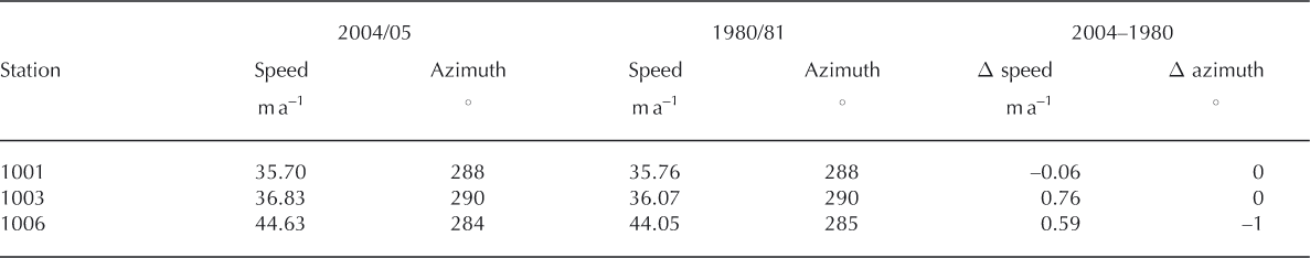
As part of the PARCA program (Reference ThomasThomas and others, 2000), three velocity measurements were made within 5–20 km of the original OSU lower cluster sites in 1996/97 (Reference Van der Veen, Jezek, Mosley-Thompson, Whillans and BolzanVan der Veen and others, 2000, Fig. 31). Because of the spatial displacement between observation sites, Reference Van der Veen, Jezek, Mosley-Thompson, Whillans and BolzanVan der Veen and others (2000) suggested that velocities had not changed over the 15 year period or at best the changes were small. Table 1 lists velocities for the 2003/04 and 1980/81 intervals at the western cluster. As noted, the aluminum marker poles at all of these locations tilted during the 2003/04 season and so a correction based on the tilt was applied. Speed errors are estimated to be ~1ma^_1 because of the uncertainty in the tilt correction, so no trend lines are inferred. However there is a weak suggestion that speeds increased at two of the stations (1003 and 1006)

Table 1.

Western cluster velocity

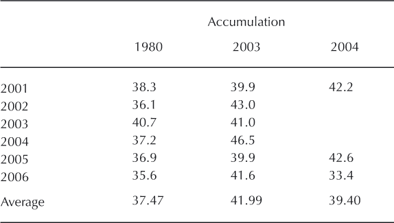
Accumulation was estimated at several central cluster sites by remeasuring aluminum pole heights above the surface. Pole height changes were converted to annual water equivalent using near-surface pit density data. The firn-core-derived results from Reference WhillansWhillans and others (1987) and later revised by Reference Van der Veen, Mosley-Thompson, Jezek, Whillans and BolzanVan der Veen and others (2001) along with the results from 2003 and 2004 are shown in Table 2. Averaged over the ice sheet, interannual variability of accumulation rate is >6cmw.e. a^-1 and higher still in the south (Reference BurgessBurgess and others, 2010), so a trend cannot be strictly inferred from this limited sampling. Note only that the later observations are 2–4 cm a^-1 higher than the earlier data.

Table 2.

Central cluster accumulation rate (cmw.e. a¹)

Accumulation data were collected at the western and Dye 3 networks during the 1980 and 1981 campaigns. Average accumulation was 38.6cmw.e. a^-1 at the western cluster and 43.1 cmw.e. a^-1 at three sites that straddle the divide at Dye 3 (Reference Van der Veen, Mosley-Thompson, Jezek, Whillans and BolzanVan der Veen and others, 2001). These spatial accumulation rate patterns are similar to those modeled by Reference Cullather and BosilovichCullather and Bosilovich (2011, Fig. 7).

Discussion

The OSU network traverses two different glacial regimes. West of the ice divide, ice flows approximately northwest towards its termination on the ice-free land. East of the ice divide, ice channels into an outlet glacier that drains into Pikiutdleq Bay (Fig. 6) where coastal glaciers are known to be thinning.

Stations west of the ice divide

Here the ice sheet above 1800m thickened at least up till 2005. This is attributable to net mass gain as suggested by Reference Kostecka and WhillansKostecka and Whillans (1988), who found a positive balance of 0.06 ± 0.08 m a^-1 for the average thickening in the vicinity of the OSU measurements west of the ice divide, and also by Reference ThomasThomas and others (2000) who found thickening of ~0.066 m a^-1. Similarities between the two flux-estimated thickness trends and those reported here (0.10 and 0.08 ± 0.02 ma^-1 for western and central clusters, respectively) indicate that the surface data are dominated by net changes in total mass rather than short-term interannual fluctuations in firn column density, at least for the period prior to about 2005.

After about 1998, there is a gradual, eastward-trending, thinning signature with time at the western cluster. This is likely due to the fact that surface melt is steadily increasing across Greenland, which contributes to significant mass loss in southern Greenland (Reference ZwallyZwally and others, 2011). Because most of southern Greenland experiences some period of melt, Reference BhattacharyaBhattacharya (2010) analyzed melt onset, end and duration for sectors distributed about Greenland. His analysis of the sectors containing the OSU western and central cluster sites shows that melt duration nearly doubled from 1978 to 2005, though the increase was roughly linear (0.81 ± 0.17 melt days a^-1). Melt occurred over 100% of the study area between 1985 and 1991 and from 1997 till the end of his analysis in 2008. Even though this portion of the ice sheet terminates on a less dynamic landward margin, the consequence of increased melt is a net thinning of the ice sheet in the ablation zone. Reference Wang, Li and ZwallyWang and others (2012) address the question of how a thickness perturbation in the ablation zone will influence the behavior of the ice sheet upstream. They find that thinning propagates upstream over time-spans on the order of a decade. Consequently, it is tempting to speculate that the thinning progression observed at the western cluster and the change in thickening rate at the central cluster are attributable to a thickness perturbation propagating inland from the ablation zone. Although the data presented here preclude a definitive conclusion on that point, the model predictions and observations to date are consistent and argue for the importance of continued measurements across the ice sheet as well as around the more dynamic margins.

Coincident with thickening at the central cluster, the surface velocity increased. An increase in velocity results from an increase in the driving stress or a decrease in other resistive stresses. For an ice sheet frozen to the bed, the driving stress is related to the surface slope. The available data enable us to investigate whether the measured velocity increases in the central cluster are consistent with changes in the driving stress. Assuming laminar flow and a frozen bed, the surface velocity U_s is given by

(1)

where n is the flow law exponent taken to be 3, ρ is the density, g is the gravitational acceleration, H is the ice thickness and ∂h/ ∂x is the slope

The variation in slope for a given variation in velocity is

(2)

Over the 25 year period the surface speed increases by no more than ~1ma^_1, and taking the local slope to be 0.006 the corresponding change in slope over 25 years is 0.0009–0.0002, depending on the choice of hardness parameter, A, selected here to be either 7 x 10^-18 or 2 x 10^-18 Pa^-3 a^-1, depending on choice of an average temperature between –20°C and –25°C (Reference Van der VeenVan der Veen, 1999, Fig. 2.6, p. 17). Now the change in slope along a length Δx of flow is

(3)

where Δh₀ is the change in elevation at the downstream end of the flowline and Δh_i is the change at the upstream end. Stations 2002 and 2005 are roughly situated along the flowline and ~40km apart. For the change in slope noted above, the difference between the changes in output and input elevation should be between 36 and 10 m, again depending on our choice of A. The difference from Figure 4 is at most 0.5 m, which in this case actually flattens the ice sheet, as confirmed by direct inspection of the 1994–2011 repeat flight described in Figure 6, which also shows negligible slope change and implies negligible change in driving stress.

The central cluster is located far from important shearing margins, arguing against a change in lateral drag. Similarly, it seems unlikely that a change in basal drag through increased basal melting is responsible for the velocity increase in regions where ice thicknesses approach 2000 m. Left are changes in longitudinal stress which seem to be the most plausible agent given the dramatic changes occurring about all of coastal Greenland (Reference Wang, Li and ZwallyWang and others, 2012).

Given the increase in velocity west of the divide, one might expect ice-sheet thinning to result from increased longitudinal flux. Yet thickening seems to coincide with velocity increase. To investigate this observation, consider the contribution of long-term increasing accumulation rate to the increasing velocity. Written in terms of flux gates, the continuity equation for each observation epoch is

(4)

The thickening rate at the central cluster was roughly constant over the period of the 1980–2005 observations, i.e. the time rate of thickness change is negligible so we can then relate time rates of velocity change to time rates of accumulation change. We do this by separately writing Eqn (4) using the parameters for each epoch, differencing the resulting two equations and setting the difference to zero. To get an analytic expression for determining the equivalent speed change for a given accumulation rate change, specify a flowband of width w₁ at the ice divide to the central cluster where the flowband width is w₂. Approximate the flowband by an isosceles trapezoid to get a rough analytic estimate of area. Assume uniform accumulation rates over the entire study area. Further assume the position of the ice divide has remained fixed and the velocity at the ice divide is close to zero. This leads to a rough estimate for the change in speed (sp) with a change in accumulation rate at the central cluster:

(5)

where L is the distance from the central cluster (~47km) to the ice divide, H is the thickness at the central cluster (~1900m) and the ratio of the flowband widths is ~0.7 (Fig. 6). Taking the total change in accumulation rate over the 25 year period to be ~0.04 m a^-1 from the limited in situ accumulation data, but which is consistent with the 1958–2007 surface mass-balance trend presented by Reference EttemaEttema and others (2009) but smaller in magnitude, the total change in speed is ~0.8ma^-1 over the same period. This is slightly faster than observed, but given the simplifying assumptions, the estimate plausibly argues that long-term accumulation rate increases sufficiently to compensate the ice thickness for the increase in ice speed.

Conclusions

Through about 2005, the interior south-central Greenland ice sheet west of the ice divide thickened. Even as the ice sheet thickened, local velocities increased. Starting perhaps as early as 1998, the most westerly sites started to thin and elevations at the central cluster sites were negligibly changed. Western thinning is a likely consequence of increased melt in the ablation zone, which may result in the upstream propagation of a thickness perturbation as described by Reference Wang, Li and ZwallyWang and others (2012).

Thinning rates increased with eastward distance from the ice divide till about 2005. Thinning is partly driven by decreasing accumulation rate trends and dynamic processes at the coast. There is now indication for a slowdown in thinning rates at most stations east of the divide and thickening at two of the stations closest to the divide.

The simpler ice dynamics at the divide and in the interior ice sheet (e.g. negligible lateral shear) means that elevation measurements there can be less dense than at the coast, where spatially complex and often rapid elevation changes are occurring. Nevertheless, and complementary to the modeling results by Reference Wang, Li and ZwallyWang and others (2012), these results show that the Greenland ice sheet is changing from terminus to divide, and measurement strategies designed to predict future changes and to estimate volumetric changes across the ice sheet need to appropriately cover the entirety of the ice sheet.