

1. Introduction
Variable annuities (VAs) have a global appeal as a retirement vehicle considering their investment innovation features and tax-deferred characteristics. A VA, also referred to as segregated funds in Canada, represents a long-term contractual arrangement between a policyholder and an insurer, structured to secure post-retirement income. Upon contract initiation, the policyholder commits to remitting either a single lump sum premium or a series of periodic premiums to the insurer. Subsequently, the premium is invested in an investment fund selected by the policyholder, which is then managed by the insurer or a third-party mutual fund manager during the accumulation phase. Upon reaching the maturity date, typically coinciding with retirement age, the policyholder possesses the flexibility to convert the accrued fund value into a life annuity or withdraw the entire fund at its prevailing market value.
In contrast to conventional fixed annuities, which provide limited returns and highly sensitive to inflation, VAs offer policyholders potential for enhanced investment outcomes through equity participation. Indeed, the presence of market volatility has also spurred a growing demand for investment protection products. VAs effectively address this need by offering a downside protection against equity market’s negative performance and interest rate fluctuations through the inclusion of guarantee riders, which are available for an additional fee. Notable variations of guarantee riders include guaranteed minimum death benefits (GMDB), guaranteed minimum maturity benefits (GMMB), guaranteed minimum accumulation benefits (GMAB), guaranteed minimum income benefits (GMIB) and guaranteed minimum withdrawal benefits (GMWB). For an in-depth examination of variable annuities and the intricacies associated with guarantee riders, interested readers are referred to the works of Hardy (Reference Hardy2003) and Ledlie et al. (Reference Ledlie, Corry, Finkelstein, Ritchie, Su and Wilson2008).
The surge in annuity sales in recent years, particularly following the pandemic-induced economic uncertainties, reflects a growing preference for risk-mitigated retirement solutions amidst volatile markets. Whilst macroeconomic conditions have been volatile, with inflationary pressures and interest rate fluctuations, this instability has amplified demand for financial safeguards. As reported by the Life Insurance Marketing and Research Association (LIMRA) (LIMRA, 2025), total U.S. annuity sales reached $432.4 billion in 2024, representing a 12% year-over-year increase, indicating sustained investors’ desire for risk-managed retirement solutions. Moreover, the LIMRA’s forecast suggests a promising trajectory for traditional VA sales in the coming years. In 2024, VA sales amounted to $61.2 billion, a 19% increase from 2023 levels, signaling a recovery from pandemic-era lows and signaling renewed investor appetite for products that combine guaranteed income floors with market participation opportunities.
Undoubtedly, the accurate valuation of as well as understanding the various risks associated with the guarantee riders embedded in the VA is of significant importance for insurers and regulators. An area of study related to the valuation and hedging of these guaranteed benefits has been evolving. Milevsky and Posner (Reference Milevsky and Posner2001) used the risk-neutral valuation method to calculate the fair value of the GMDB in a VA and death-protected mutual funds. In Gerber et al. (Reference Gerber, Shiu and Yang2012), a discounted density approach is introduced in valuing the GMDB for which a closed form solution is obtained. A partial-differential-equation-based method is developed in Bélanger et al. (Reference Bélanger, Forsyth and Labahn2009) to determine the fair charge rate for GMDB with a partial withdrawal feature. Shen et al. (Reference Shen, Sherris and Ziveyi2016) proposed a numerical-integration-based approach for the valuation of the GMMB in VA with surrender options, for which an explicit integral expression is established. A modelling framework incorporating regime-switching and stochastic mortality for valuing and hedging of the GMMB and GMDB is developed in Ignatieva et al. (Reference Ignatieva, Song and Ziveyi2016).
Further developments could be found in Bernard et al. (Reference Bernard, MacKay and Muehlbeyer2014) where a new fee structure, called the state-dependent fee, was considered for the valuation of GMMB and GMDB. Whilst in Cui et al. (Reference Cui, Feng and MacKay2017), the VIX-linked fee structure for the valuation of GMMB, under a Heston volatility model, was studied. Huang et al. (Reference Huang, Mamon and Xiong2022) proposed a modelling framework incorporating three correlated risk factors for the valuation of the GMAB. The paper of Bacinello et al. (Reference Bacinello, Millossovich, Olivieri and Pitacco2011) attempted to put forward a unifying framework for the valuation of several guaranteed riders. Hyndman and Wenger (Reference Hyndman and Wenger2014) investigated the pricing and hedging of the GMWB rider from a financial economic perspective. The GMWB valuation incorporating step-up, bonus, and surrender features in a low interest rate environment was examined in Fontana and Rotondi (Reference Fontana and Rotondi2023).
This paper aims to give a novel contribution to the valuation of the GMIB, which is a highly sought-after type of guarantee rider. The GMIB rider is a particularly attractive investment feature to policyholders due to the following reasons: (i) It provides protection against longevity risk. With advancements in medical and health sciences substantially augmenting life expectancy in recent decades, individuals are increasingly concerned about the possibility of outliving their retirement income. By granting policyholders the option to convert their retirement savings into a life annuity, the GMIB effectively transfers the longevity risk to insurers. (ii) There is provision of stable payments irrespective of market performance. The GMIB ensures a guaranteed minimum income upon annuitisation, thereby shielding policyholders from the adverse impact of market volatility or fluctuations in interest rates. This steady income stream aids in covering essential expenses and maintaining a desired standard of living during retirement. (iii) An equitable market participation, with downside protection, is achieved. Through the GMIB, policyholders have the opportunity to capitalise on equity market growth during prosperous periods, whilst simultaneously benefiting from the security of a guaranteed minimum level of annuity payments at maturity. (iv) The last but not least salient characteristic of the GMIB rider is transparency. The GMIB equips policyholders with precise knowledge regarding the predetermined guaranteed minimum payments at each age, simplifying retirement planning endeavours.
A comparable product existing in the European market is the guaranteed annuity option (GAO), which shares certain similarities with the GMIB. The valuation and hedging of the GAO have been extensively explored by various authors. See, for example, Boyle and Hardy (Reference Boyle and Hardy2003), Liu et al. (Reference Liu, Mamon and Gao2013, Reference Liu, Mamon and Gao2014), Ballotta and Haberman (Reference Ballotta and Haberman2003), Pelsser (Reference Pelsser2003), and Zhao et al. (Reference Zhao, Mamon and Gao2018), amongst others. Both the GMIB and GAO offer a guaranteed conversion rate upon annuitisation. However, the GMIB distinguishes itself from the GAO in terms of product design and benefit structure, necessitating a distinct dependence modelling approach. The structural divergence between GMIB and GAO stems from their distinct risk absorption capacities and contractual obligations. GMIBs integrate tripartite risk hedging through dynamic mechanisms: market risk is mitigated via the downside protection afforded by the rider’s contractual features (Marshall et al., Reference Marshall, Hardy and Saunders2010), longevity risk is pooled through mortality credits (Zhou et al., Reference Zhou, Garces, Shen, Sherris and Ziveyi2025), and interest rate exposure is managed via duration-matching strategies (Ignatieva et al., Reference Ignatieva, Song and Ziveyi2016). This contrasts sharply with GAOs, which primarily guarantee annuity conversion rates at maturity without intervening in accumulation-phase risks, leaving policyholders exposed to market volatility and longevity uncertainties throughout the contract term. Empirical analyses of insurer reserving practices (Chahboun and Hoover, Reference Chahboun and Hoover2019) confirm that GMIB liabilities incorporate actuarial adjustments for all three risks, whereas GAO reserves primarily reflect interest rate sensitivity.
This dichotomy necessitates a framework capable of capturing the nonlinear interactions between market, longevity, and interest rate factors unique to GMIBs. Insights derived from GAO models, often reliant on static rate hedging assumptions, are not readily adaptable in tackling these complex interactions. In contrast, our study delivers novel insights by: (i) quantifying the material impact of correlated interest-mortality risks specifically within the GMIB’s multi-risk structure, revealing distinct sensitivity patterns; (ii) demonstrating the critical role of stochastic mortality dependence for accurate GMIB valuation, where its exclusion leads to significant overpricing; and (iii) developing a tailored numéraire transformation technique that efficiently handles the joint survival contingency, path-dependent guarantees, and correlated risks inherent to GMIBs, achieving computational efficiency unattainable with standard GAO valuation methods. Consequently, a distinct and targeted analysis for the GMIB is therefore not only necessary but yields product-specific insights critical for insurer risk management and pricing.
Bauer et al. (Reference Bauer, Kling and Russ2010) formulated a general framework that could be used to evaluate a variety of guarantees offered within the VA context in a consistent way. Their model framework was based on the assumption that the investment fund model is given by a geometric Brownian motion with a constant interest rate, incorporating a deterministic mortality model based on the mortality table of the German Society of Actuaries. Later, Marshall et al. (Reference Marshall, Hardy and Saunders2010) extended the Bauer et al.’s framework (Bauer et al., Reference Bauer, Kling and Russ2010) by allowing the interest rate to follow the stochastic Hull–White model. They considered the valuation of GMIB in more detail and a variety of GMIB’s contract designs was elaborated. In order to evaluate the GMIB in a complete market and thereafter focus on the financial risks, they did not take mortality into account in their valuation. However, in practice, the GMIB often offers a life-related annuity; therefore, the longevity risk, which is a non-diversifiable risk must be incorporated into the valuation of the GMIB. Additionally, Deelstra and Rayée (Reference Deelstra and Rayée2013) studied the valuation of the GMIB in a local volatility model setting. Their model is an extension of that in Marshall et al. (Reference Marshall, Hardy and Saunders2010) with the inclusion of a stochastic local volatility into the investment fund model. It is assumed that the survival rates were calculated based on a mortality table, which is an acceptable assumption over the short term. But for the VA with maturities of at least 10 years, the mortality intensity needs to be modelled stochastically to capture the uncertainty related to mortality evolution in the long run.
Various stochastic models were developed and analysed in predicting mortality rates. Lee and Carter (Reference Lee and Carter1992) introduced a relatively robust one-parameter model that closely describes the trends observed in the U.S. population data. An evaluation of eight stochastic models concerning mortality forecasts at advanced ages was conducted by Cairns et al. (Reference Cairns, Blake, Dowd, Coughlan, Epstein, Ong and Balevich2009). Luciano and Vigna (Reference Luciano and Vigna2008) undertook the calibration of affine models to different generations within the UK population, assessing their empirical adequacy. Their analysis concluded that non-mean reverting Ornstein-Ulhenbeck processes offer a suitable framework for characterising human mortality. Subsequently, the study of Zeddouk and Devolder (Reference Zeddouk and Devolder2020) zeroed in on four distinct types of stochastic processes tailored to the Belgian population. Their findings indicated that mean reversion models, incorporating a variable target associated with the age-related increase in mortality, outperform non-mean reversion models. In this paper, we adopt the mortality rate model proposed by Zeddouk and Devolder (Reference Zeddouk and Devolder2020) as the foundation of our analysis.
In the actuarial literature, the prevalent assumption regarding the valuation of insurance products often entails the independence of mortality risk from interest risk. However, as expounded by Dhaene et al. (Reference Dhaene, Kukush, Luciano, Schoutens and Stassen2013), maintaining this observed real-world relationship between mortality and interest risks within the risk-neutral domain is frequently unattainable. The studies by Miltersen and Persson (Reference Miltersen and Persson2005) and Liu et al. (Reference Liu, Mamon and Gao2014) demonstrated that the influence of mortality risk on the economy could subsequently impact interest rate movements. Moreover, Deelstra et al. (Reference Deelstra, Grasselli and Van Weverberg2016) emphasised the substantial implications of the dependence between mortality and interest risks on the evaluation of insurance products. Consequently, there is merit in establishing a mathematical framework that accommodates a dependence structure between these two risks.
Actuarial practice demands a valuation methodology that accurately captures the dynamics and risk dependence and simultaneously remains practical for implementation and adaptable to existing insurance pricing infrastructures. This paper responds to this necessity by developing a valuation framework for the GMIB. The key contributions of this study are as follows: (i) Reflecting reality, where market risks and uncertainties must be modelled adequately, into a risk-neutral valuation framework, we provide further developments in constructing equivalent martingale measures with some parallel to the method in Dahl and Møller (Reference Dahl and Møller2006). (ii) We introduce a modelling structure for valuing the GMIB rider, incorporating correlated stochastic interest and mortality rates, expanding upon the settings explored in Bauer et al. (Reference Bauer, Kling and Russ2010) and Marshall et al. (Reference Marshall, Hardy and Saunders2010). (iii) By introducing the endowment-risk-adjusted measure, we derive an analytical solution for the GMIB rider, exploring two distinct Benefit Base function scenarios. (iv) A computational algorithm is presented for the GMIB valuation, where the standard Monte Carlo simulation and our proposed method are compared. Numerical results showcase the efficacy of our approach in accurately valuing GMIB with significantly reduced computation time, when benchmarked to the standard Monte Carlo simulation. (v) We conduct a sensitivity analysis to assess the impact of various model parameters on GMIB valuation, offering valuable insights for insurers in decision-making processes. (vi) The flexibility of our modelling framework and the application of the change of numéraire approach could be extended to evaluate other types of guarantee riders, enhancing its practical utility within the insurance industry.
The remainder of this paper is structured as follows. In Section 2, we present our proposed modelling framework used to value the GMIB. Section 3 discusses the main characteristics of the GMIB and lists the assumptions for the GMIB valuation. Our proposed numéraire transformation technique is introduced in Section 4. More specifically, the forward measure and the endowment-risk-adjusted measure are constructed to obtain an analytical solution for the GMIB. A numerical experiment is presented in Section 5 to assess the accuracy and efficiency of our proposed methodology. We also provide a sensitivity analysis to examine the influence of various parameters on the GMIB value. Finally, Section 6 concludes this paper.
2. Modelling framework
There are three uncertainty risks associated with the valuation of the GMIB, namely, the interest rate $r_t$
, the mortality intensity
$r_t$
, the mortality intensity $\mu_t$
, and the investment fund
$\mu_t$
, and the investment fund $S_t$
. We assume that these three processes are defined on a filtered probability space
$S_t$
. We assume that these three processes are defined on a filtered probability space $(\Omega,\mathcal{F},\{\mathcal{F}_{t}\},P)$
, where
$(\Omega,\mathcal{F},\{\mathcal{F}_{t}\},P)$
, where $\{\mathcal{F}_{t}\}$
represents the joint filtration generated by
$\{\mathcal{F}_{t}\}$
represents the joint filtration generated by $r_{t}$
,
$r_{t}$
, $\mu_{t}$
, and
$\mu_{t}$
, and $S_t$
, with P denoting an objective probability measure. The concepts of risk-neutral and real-world measures hold significant importance within the realm of financial mathematics. The risk-neutral measure serves as a theoretical probability measure for the valuation of financial products, where investors exhibit indifference towards risk. Conversely, the real-world measure encapsulates the authentic market risks and uncertainties. When valuing a contingent claim under the risk-neutral measure, some robust mathematical characteristics and tools could be employed. This assumption simplifies the mathematical modelling process under the risk-neutral measure and facilitates the application of valuation techniques. In order to relate the risk-neutral and real-world measures, a suitable density is defined so that risk-adjusted probabilities are obtained. This measure-change transition ensures that the valuation of a GMIB incorporates genuine market risks. The explicit procedure for effectuating the change of measure from the real-world measure P to a risk-neutral measure Q is included in Appendix A.
$S_t$
, with P denoting an objective probability measure. The concepts of risk-neutral and real-world measures hold significant importance within the realm of financial mathematics. The risk-neutral measure serves as a theoretical probability measure for the valuation of financial products, where investors exhibit indifference towards risk. Conversely, the real-world measure encapsulates the authentic market risks and uncertainties. When valuing a contingent claim under the risk-neutral measure, some robust mathematical characteristics and tools could be employed. This assumption simplifies the mathematical modelling process under the risk-neutral measure and facilitates the application of valuation techniques. In order to relate the risk-neutral and real-world measures, a suitable density is defined so that risk-adjusted probabilities are obtained. This measure-change transition ensures that the valuation of a GMIB incorporates genuine market risks. The explicit procedure for effectuating the change of measure from the real-world measure P to a risk-neutral measure Q is included in Appendix A.
2.1. Interest rate model
Under Q, the interest rate $r_t$
follows the Hull–White model (Hull and White, Reference Hull and White1990)
$r_t$
follows the Hull–White model (Hull and White, Reference Hull and White1990)
 \begin{equation} \mathrm{d}r_{t}=a(\theta(t)-r_{t})\mathrm{d}t+\sigma_1 \mathrm{d}X_{t}{.}\end{equation}
In Equation (2.1), a and $\sigma_1$
are positive constants,
$\sigma_1$
are positive constants, $\theta(t)$
is a deterministic function describing the initial term structure of the interest rates, and
$\theta(t)$
is a deterministic function describing the initial term structure of the interest rates, and $X_{t}$
is a standard Brownian motion (BM). Consequently, under the Hull–White set up, the price B(t, T) of a T-maturity zero-coupon bond at time
$X_{t}$
is a standard Brownian motion (BM). Consequently, under the Hull–White set up, the price B(t, T) of a T-maturity zero-coupon bond at time $t \lt T$
(cf Mamon, Reference Mamon2004) is given by
$t \lt T$
(cf Mamon, Reference Mamon2004) is given by
 \begin{equation}B(t, T)=\mathbb{E}^{Q}\big[e^{-\int_{t}^{T}r_{u} \mathrm{d}u} \big|\mathcal{F}_{t}\big]=e^{-A(t, T)r_{t}+D(t, T)},\end{equation}
where
 \begin{align*}A(t, T)=\frac{1-e^{-a(T-t)}}{a}\qquad\end{align*}
and
 \begin{align*}D(t, T)=-\int_{t}^{T}{\left( 1-e^{-a(T-u)}\right) \theta(u)\mathrm{d}u}+\frac{\sigma_1^2}{4a^3}\left[2a(T-t)-3+4e^{-a(T-t)}-e^{-2a(T-t)}\right].\end{align*}
2.2. Mortality model
Let $\mu_{x,t}$
be the time-t force of mortality of an individual aged x at time 0. We assume that
$\mu_{x,t}$
be the time-t force of mortality of an individual aged x at time 0. We assume that $\mu_{x,t}$
also follows the Hull–White specification (Hull and White, Reference Hull and White1990)
$\mu_{x,t}$
also follows the Hull–White specification (Hull and White, Reference Hull and White1990)
 \begin{equation} \mathrm{d}\mu_{x,t}=c( \xi(t)-\mu_{x,t}) \mathrm{d}t+\sigma_2 \mathrm{d}Y_{t},\end{equation}
where c and $\sigma_2$
are positive constants,
$\sigma_2$
are positive constants, $\xi(t)$
is a deterministic function, and
$\xi(t)$
is a deterministic function, and $Y_{t}$
is a standard BM. In respect of mortality modelling, the parameters of Equation (2.3) could be set in such a way that the probability for
$Y_{t}$
is a standard BM. In respect of mortality modelling, the parameters of Equation (2.3) could be set in such a way that the probability for $\mu_{x,t}$
to ever become negative is minimised.
$\mu_{x,t}$
to ever become negative is minimised.
As argued in Liu et al. (Reference Liu, Mamon and Gao2013), the impact of mortality risk on the economy could subsequently influence the movement of interest rates. Therefore, it is advantageous to establish a mathematical framework that accommodates a dependence structure between these two risks. To this end, we suppose that $X_t$
and
$X_t$
and $Y_t$
are correlated and their dependence is modelled as
$Y_t$
are correlated and their dependence is modelled as $\mathrm{d}X_t \mathrm{d}Y_t= \rho \mathrm{d}t$
.
$\mathrm{d}X_t \mathrm{d}Y_t= \rho \mathrm{d}t$
.
Following Zeddouk and Devolder (Reference Zeddouk and Devolder2020), we posit that $\xi(t)$
conforms to the Gompertz function, expressed as
$\xi(t)$
conforms to the Gompertz function, expressed as $\xi(t)=pe^{ht}$
, signifying the exponential growth of the mortality intensity with advancing age. Here, p denotes the baseline mortality at age x, whilst h represents the senescent component. To streamline the notation, we shall omit the age index x and exclusively employ the notation
$\xi(t)=pe^{ht}$
, signifying the exponential growth of the mortality intensity with advancing age. Here, p denotes the baseline mortality at age x, whilst h represents the senescent component. To streamline the notation, we shall omit the age index x and exclusively employ the notation $\mu_{t}$
throughout the subsequent sections of this paper.
$\mu_{t}$
throughout the subsequent sections of this paper.
Notably, both the interest rate and mortality models in our framework adopt the Hull–White specification. This choice is not dismissive of alternative models (e.g., the Lee–Carter model). Rather, such a choice is motivated by the fact that our framework necessitates a specific mathematical structure to achieve tractable valuation of the GMIB rider. The Lee–Carter model, despite its empirical robustness for mortality forecasting, is incompatible with our objectives for two fundamental reasons: (i) Our valuation framework requires explicit continuous-time modelling of the dependence between interest rate risk and mortality risk, captured through correlated Brownian motions. The standard Lee–Carter model, being inherently discrete-time, does not readily accommodate such a correlated diffusion framework. (ii) The derivation of analytical solutions via the numéraire transformation approach in Section 4 critically depends on the mortality process belonging to the affine model class. The Hull–White specification satisfies this: its mortality intensity has linear drift and diffusion terms relative to its state variable, ensuring the Radon–Nikodym derivative for the endowment-risk-adjusted measure admits a closed-form solution, an essential prerequisite for proving Theorems 4.1 and 4.2. Standard Lee–Carter implementations, even in continuous-time variants, generally lack the required affine structure, which would render the Radon–Nikodym derivative intractable and hamper the measure transformation technique central to our methodology. Therefore, the selection of the Hull–White model for mortality is not merely a matter of preference but a structural modelling necessity. Its affine form and compatibility with correlated diffusions are indispensable for deriving closed-form expressions under the endowment-risk-adjusted measure, enabling the computationally efficient valuation presented in Section 5.
2.3. Investment fund model
We assume that the investment fund $S_t$
of a VA follows the geometric Brownian motion
$S_t$
of a VA follows the geometric Brownian motion
 \begin{equation*} \mathrm{d}S_{t}=r_t S_t\mathrm{d}t +\sigma_3 S_t \mathrm{d}Z_{t},\end{equation*}
where $\sigma_3$
is a positive constant, and
$\sigma_3$
is a positive constant, and $Z_{t}$
is a standard BM independent of
$Z_{t}$
is a standard BM independent of $X_t$
and
$X_t$
and $Y_t$
. The assumption of independence is a deliberate simplification grounded in methodological focus. Although correlations between equity returns and interest rates are well-documented (e.g., Zaremba et al., Reference Zaremba, Cakici, Bianchi and Long2023), our baseline model explicitly assumes independence between the investment fund and the interest rate for three reasons: (i) This assumption emphasises isolating the underexplored interdependence between mortality and interest risks in insurance valuation, particularly for products with longevity exposure. The joint dynamics of mortality and interest rates in GMIBs, especially their nonlinear impact on actuarial liabilities, remain insufficiently studied. By holding equity and interest rates independent, we avoid confounding two distinct sources of risk and ensure that the mortality–interest rate interaction is clearly identified. (ii) Introducing equity–interest rate correlation would considerably complicate the model without materially altering our central conclusions. Our framework captures equity risk through the dynamics of the investment fund and the path-dependent Benefit Base in Section 3. Adding a correlated equity–interest rate process would require a three-dimensional stochastic system, increasing computational burden whilst diverting focus from the numéraire transformation technique’s efficiency. (iii) GMIBs are primarily designed to hedge policyholders against longevity, interest rate, and equity risks, rather than equity-interest rate covariation, with Marshall et al. (Reference Marshall, Hardy and Saunders2010) noting the relatively minor influence of the equity-interest rate correlation on GMIB value. Moreover, equity risk is partially retained by the policyholder through the fund selection, with downside protection provided by the Benefit Base.
$Y_t$
. The assumption of independence is a deliberate simplification grounded in methodological focus. Although correlations between equity returns and interest rates are well-documented (e.g., Zaremba et al., Reference Zaremba, Cakici, Bianchi and Long2023), our baseline model explicitly assumes independence between the investment fund and the interest rate for three reasons: (i) This assumption emphasises isolating the underexplored interdependence between mortality and interest risks in insurance valuation, particularly for products with longevity exposure. The joint dynamics of mortality and interest rates in GMIBs, especially their nonlinear impact on actuarial liabilities, remain insufficiently studied. By holding equity and interest rates independent, we avoid confounding two distinct sources of risk and ensure that the mortality–interest rate interaction is clearly identified. (ii) Introducing equity–interest rate correlation would considerably complicate the model without materially altering our central conclusions. Our framework captures equity risk through the dynamics of the investment fund and the path-dependent Benefit Base in Section 3. Adding a correlated equity–interest rate process would require a three-dimensional stochastic system, increasing computational burden whilst diverting focus from the numéraire transformation technique’s efficiency. (iii) GMIBs are primarily designed to hedge policyholders against longevity, interest rate, and equity risks, rather than equity-interest rate covariation, with Marshall et al. (Reference Marshall, Hardy and Saunders2010) noting the relatively minor influence of the equity-interest rate correlation on GMIB value. Moreover, equity risk is partially retained by the policyholder through the fund selection, with downside protection provided by the Benefit Base.
To ensure a consistent correlation matrix when generating $X_t$
,
$X_t$
, $Y_t$
, and
$Y_t$
, and $Z_t$
for simulation and other financial modelling purposes, the relation dynamics of these BMs are defined in the following manner:
$Z_t$
for simulation and other financial modelling purposes, the relation dynamics of these BMs are defined in the following manner:
 \begin{align*}\mathrm{d}X_{t} = \mathrm{d}W_{t}^{1}, \, \mathrm{d}Y_{t} = \rho\mathrm{d}W_{t}^{1}+\sqrt{1-\rho^{2}}\mathrm{d}W_{t}^{2},\, \mbox{and} \, \mathrm{d}Z_{t} = \mathrm{d}W_{t}^{3}, \end{align*}
where $W_{t}^{1}$
,
$W_{t}^{1}$
, $W_{t, }^{2}$
and
$W_{t, }^{2}$
and $W_{t}^{3}$
are independent standard BMs.
$W_{t}^{3}$
are independent standard BMs.
To verify the rationality of our baseline assumption, we relax the independence assumption in a dedicated extended setting by incorporating equity-interest correlation, specifying the correlation structure of the three-dimensional risk factors as: $\mathrm{d} X_t \mathrm{d}Y_t=\rho \mathrm{d}t$
,
$\mathrm{d} X_t \mathrm{d}Y_t=\rho \mathrm{d}t$
, $\mathrm{d} X_t \mathrm{d}Z_t=\rho^* \mathrm{d}t$
and
$\mathrm{d} X_t \mathrm{d}Z_t=\rho^* \mathrm{d}t$
and $\mathrm{d} Y_t \mathrm{d}Z_t=0$
. The assumption of
$\mathrm{d} Y_t \mathrm{d}Z_t=0$
. The assumption of $\mathrm{d} Y_t \mathrm{d}Z_t=0$
is reasonable given existing findings. Whilst systemic longevity improvements might exhibit a weak long-run relationship with macroeconomic factors that influence equity returns, the immediate, direct correlation between mortality shocks and equity market fluctuations is generally considered negligible for valuation purposes (Arik et al., Reference Arık2023). As noted in Hanewald (Reference Hanewald2011), mortality evolution is primarily driven by long-term trends in healthcare, lifestyle, and medical technology, whereas equity returns are influenced by a different set of short- to medium-term economic, political, and market-specific factors. This extension maintains the core structure of mortality-interest rate interactions and the numéraire transformation logic, ensuring consistency with the baseline framework. To model the dependence structure, the correlated BMs
$\mathrm{d} Y_t \mathrm{d}Z_t=0$
is reasonable given existing findings. Whilst systemic longevity improvements might exhibit a weak long-run relationship with macroeconomic factors that influence equity returns, the immediate, direct correlation between mortality shocks and equity market fluctuations is generally considered negligible for valuation purposes (Arik et al., Reference Arık2023). As noted in Hanewald (Reference Hanewald2011), mortality evolution is primarily driven by long-term trends in healthcare, lifestyle, and medical technology, whereas equity returns are influenced by a different set of short- to medium-term economic, political, and market-specific factors. This extension maintains the core structure of mortality-interest rate interactions and the numéraire transformation logic, ensuring consistency with the baseline framework. To model the dependence structure, the correlated BMs $\{X_t, Y_t, Z_t\}$
can be constructed through Cholesky decomposition:
$\{X_t, Y_t, Z_t\}$
can be constructed through Cholesky decomposition:
 \begin{align*}\mathrm{d}X_{t} = \sqrt{1-\rho^{2}-(\rho^*)^{2}} \mathrm{d}W_{t}^{1}+ \rho \mathrm{d}W_{t}^{2}+\rho^* \mathrm{d}W_{t}^{3},\, \mathrm{d}Y_{t} =\mathrm{d}W_{t}^{2}, \, \text{and} \, \mathrm{d}Z_{t} = \mathrm{d}W_{t}^{3},\end{align*}
where $W_{t}^{1}$
,
$W_{t}^{1}$
, $W_{t}^{2,}$
and
$W_{t}^{2,}$
and $W_{t}^{3}$
are independent standard BMs. Numerical results of the extended model are presented in Section 5.6, quantifying the impact of equity-interest correlation.
$W_{t}^{3}$
are independent standard BMs. Numerical results of the extended model are presented in Section 5.6, quantifying the impact of equity-interest correlation.
3. GMIB contract description
Consider a VA with a maturity date of T and an initial premium of $P_0$
, which is entirely invested in the policyholder’s chosen investment fund
$P_0$
, which is entirely invested in the policyholder’s chosen investment fund $S_t$
. The policyholder’s fund, denoted as
$S_t$
. The policyholder’s fund, denoted as $F_t$
and held in a separate account, is linked to the performance of the investment fund
$F_t$
and held in a separate account, is linked to the performance of the investment fund $S_t$
. Assuming a constant continuously compounded management charge rate of
$S_t$
. Assuming a constant continuously compounded management charge rate of $\alpha$
, we establish the relationship
$\alpha$
, we establish the relationship
 \begin{align*}F_t=F_0\frac{S_t}{S_0}e^{-\alpha t}, \end{align*}
where $F_0=S_0=P_0$
. By applying Itô’s lemma, the policyholder’s fund
$F_0=S_0=P_0$
. By applying Itô’s lemma, the policyholder’s fund $F_t$
satisfies
$F_t$
satisfies
 \begin{equation} \mathrm{d}F_t=({r_t-\alpha}){F_t}\mathrm{d}t +\sigma_3F_t\mathrm{d}W_t^3.\end{equation}
A GMIB rider offers a guaranteed annuitisation rate g, where g represents the annual income amount provided per unit of a lump sum. At the maturity date T, if g proves more advantageous than the prevailing market annuitisation rates, the policyholder has the option to utilise their GMIB rider. This allows them to convert a predetermined minimum sum of funds (referred to as the Benefit Base) into a life annuity at the guaranteed rate g. Conversely, if the market annuitization rates offer superior terms, the policyholder may opt to forgo the GMIB rider, withdraw their funds $F_T$
, and annuitise them at the market rate. Importantly, it is essential to highlight that the GMIB serves as a survivor benefit, meaning that annuitisation does not occur in the event of the policyholder’s demise before the maturity date T.
$F_T$
, and annuitise them at the market rate. Importantly, it is essential to highlight that the GMIB serves as a survivor benefit, meaning that annuitisation does not occur in the event of the policyholder’s demise before the maturity date T.
Let $BB_T$
be the Benefit Base in the event that the policy matures at time T. As per Marshall et al. (Reference Marshall, Hardy and Saunders2010), we adopt two variations of the Benefit Base. In Benefit Base I, the Benefit Base exhibits growth at a fixed and guaranteed rate
$BB_T$
be the Benefit Base in the event that the policy matures at time T. As per Marshall et al. (Reference Marshall, Hardy and Saunders2010), we adopt two variations of the Benefit Base. In Benefit Base I, the Benefit Base exhibits growth at a fixed and guaranteed rate $\delta$
, referred to as a roll-up feature. This can be expressed as
$\delta$
, referred to as a roll-up feature. This can be expressed as
 \begin{align*}BB_T=P_0e^{\delta T}. \end{align*}
In addition to a roll-up feature, the Benefit Base II incorporates a discrete lookback feature (this is known as a step-up guarantee in actuarial science), giving the policyholder the opportunity to lock in gains when investment returns are strong during the accumulation phase. Let $0=t_1 \lt t_2 \lt \cdots \lt t_m=T$
be some pre-selected policy anniversaries, the Benefit Base II is of the form
$0=t_1 \lt t_2 \lt \cdots \lt t_m=T$
be some pre-selected policy anniversaries, the Benefit Base II is of the form
 \begin{align*}BB_T=\max{ \left( P_0e^{\delta T}, F_{t_1}, F_{t_2}, \ldots, F_{t_m} \right)}. \end{align*}
Based on information provided by annuity issuers (My Annuity Store, 2020), the Benefit Base serves exclusively for the calculation of the guaranteed income amount at the time of annuitisation, and it is not redeemable for cash under any circumstances.
Moreover, we suppose that the guaranteed minimum income is distributed as a level annual n-year term life annuity-due for an individual life, with the first payment commencing at age $x+T$
(where T represents the passage of time). Upon procuring the GMIB, policyholders have the option to opt for either a single life policy or a joint life policy. For the purpose of this paper, we specifically focus on the single life policy, whilst acknowledging that the joint life policy is expected to further enhance the value of the GMIB. Additionally, the annuity factor could be structured as a whole life annuity, a guaranteed annuity with specific payments, or an annuity with non-level payment patterns.
$x+T$
(where T represents the passage of time). Upon procuring the GMIB, policyholders have the option to opt for either a single life policy or a joint life policy. For the purpose of this paper, we specifically focus on the single life policy, whilst acknowledging that the joint life policy is expected to further enhance the value of the GMIB. Additionally, the annuity factor could be structured as a whole life annuity, a guaranteed annuity with specific payments, or an annuity with non-level payment patterns.
Let $M(t,T^*)$
be the fair value at time t of a $1 pure endowment payable at maturity
$M(t,T^*)$
be the fair value at time t of a $1 pure endowment payable at maturity $T^*$
. Using the risk-neutral valuation, we have
$T^*$
. Using the risk-neutral valuation, we have
 \begin{equation*} M(t,T^*) = \mathbb{E}^{Q}\left[e^{-\int_{t}^{T^*}r_{u}\mathrm{d}u} e^{-\int_{t}^{T^*}\mu_{u}\mathrm{d}u} \middle |\mathcal{F}_{t}\right].\end{equation*}
The n-year term life annuity can be decomposed into a sum of pure endowments; that is,
 \begin{align*} \ddot{a}_{x+T:\overline{n\,}\!\mid}=\sum_{k=0}^{n-1}M(T,T+k).\end{align*}
Additionally, we assume that the policyholder maintains the GMIB until the maturity T, ensuring no policy lapses prior to the designated maturity date. In practical terms, unforeseen circumstances may arise for the policyholder before the annuitisation date, necessitating an immediate need for funds. Consequently, they may opt to lapse their VA contract, thereby forfeiting the guarantee rider GMIB, and withdraw their investment at the prevailing market value. Therefore, lapse risk emerges as a pivotal factor confronting insurers and entails careful consideration and mitigation. Based on Kim (Reference Kim2005), lapse risk is influenced by a myriad of variables, including interest rates, unemployment rates, macroeconomic conditions, and policy specifications. Their intricate interplay underscores the substantial challenges in accurately measuring and managing lapse risk. Nevertheless, we shall accommodate the effect of lapse risk on the GMIB value under a simplified lapse rate model in Section 5.7.
With the notations defined above, the payoff of a GMIB rider at the maturity date T, conditional on the survival of the policyholder, is expressed as
 \begin{align*}\max(BB_T g \ddot{a}_{x+T:\overline{n\,}\!\mid} -F_{T},0). \end{align*}
By the risk-neutral valuation, the fair value of a GMIB at time t is
 \begin{align} P_{\rm{\scriptsize GMIB}}(t) = \mathbb{E}^{Q} \left[e^{-\int_{t}^{T} r_{u} \mathrm{d}u} e^{-\int_{t}^{T} \mu_u \mathrm{d}u}{\max(BB_T g \ddot{a}_{x+T:\overline{n\,}\!\mid} -F_{T},0)} \middle |\mathcal{F}_{t}\right]. \end{align}
4. Derivation of GMIB value
In this section, we employ the change of measure technique to carry out the pricing evaluation of the GMIB. This is accomplished by introducing the forward measure to obtain a closed-form solution for the pure endowment M(t, T).
4.1. Forward measure
The bond price $B(t,T^*)$
, where
$B(t,T^*)$
, where $T^*$
is an arbitrary number, is chosen as a numéraire associated with the forward measure
$T^*$
is an arbitrary number, is chosen as a numéraire associated with the forward measure $\widetilde{Q}$
equivalent to the risk-neutral measure Q via the Radon-Nikodým derivative
$\widetilde{Q}$
equivalent to the risk-neutral measure Q via the Radon-Nikodým derivative
 \begin{align*} \left.\frac{\mathrm{d}\widetilde{Q}}{\mathrm{d}Q}\right|_ {\mathcal{F}_{T^*}}=\Lambda^{1}_{T^*}\, :\!=\, \frac{ e^{-\int_{0}^{T^*}r_{u}\mathrm{d}u}B(T^*,T^*)}{B(0,T^*)}. \end{align*}
By the Bayes’ rule for conditional expectation,
 \begin{equation} M(t,T^*)= \mathbb{E}^{Q}\left[e^{-\int_{t}^{T^*}r_{u}\mathrm{d}u} e^{-\int_{t}^{T^*}\mu_{u}\mathrm{d}u}\middle |\mathcal{F}_{t}\right]=B(t,T^*)\mathbb{E}^{\widetilde{Q}} \left[e^{-\int_{t}^{T^*}\mu_{u}\mathrm{d}u}\middle |\mathcal{F}_{t}\right]=B(t,T^*)S(t,T^*).\end{equation}
Our calculations show that
 \begin{equation*} \mathrm{d}\Lambda_{t}^{1}=-\sigma_1 A(t,T^*) \Lambda_{t}^{1}\mathrm{d}W_{t}^{1}.\end{equation*}
In accordance with the Girsanov’s Theorem, $\widetilde{W}_{t}^{1}$
and
$\widetilde{W}_{t}^{1}$
and $\widetilde{W}_{t}^{2}$
are standard BMs under
$\widetilde{W}_{t}^{2}$
are standard BMs under $\widetilde{Q}$
, where
$\widetilde{Q}$
, where
 \begin{align*} \mathrm{d}\widetilde{W}_{t}^{1} = \mathrm{d}W_{t}^{1}+\sigma_1 A(t,T^*)\mathrm{d}t \, \text{and} \, \mathrm{d}\widetilde{W}_{t}^{2} = \mathrm{d}W_{t}^{2}. \end{align*}
It follows that the $\widetilde{Q}$
dynamics of
$\widetilde{Q}$
dynamics of $r_{t}$
and
$r_{t}$
and $\mu_{t}$
are given by
$\mu_{t}$
are given by
 \begin{align} \mathrm{d}r_{t} &= [a\theta(t)-\sigma_1^{2}A(t,T^*)-ar_{t}]\mathrm{d}t +\sigma_1 \mathrm{d}\widetilde{W}_{t}^{1}, \, {\text{and}} \nonumber \\[3pt] \mathrm{d}\mu_{t} &= [cpe^{ht}-\rho\sigma_1\sigma_2 A(t,T^*) -c\mu_{t}]\mathrm{d}t+\sigma_2\left (\rho\mathrm{d}\widetilde{W}_{t}^{1} +\sqrt{1-\rho^{2}}\mathrm{d}\widetilde{W}_{t}^{2}\right). \end{align}
We could solve (4.2), by variation of constants, to obtain
 \begin{align} \mu_u&= \mu_te^{-c(u-t)} + \frac{cp}{c+h}\left( e^{hu} - e^{-cu+(c+h)t} \right) +\frac{\rho \sigma_1 \sigma_2 e^{-a T^*}}{a(a+c)}\left( e^{au} - e^{-cu+(a+c)t} \right) -\frac{\rho \sigma_1 \sigma_2 }{ac}\left( 1 - e^{-c(u-t)} \right) \nonumber \\[3pt] &\quad +\sigma_2 \rho e^{-cu} \int_{t}^{u}{e^{cs}\mathrm{d}\widetilde{W}_{t}^{1}} + \sigma_2 \sqrt{1-\rho^{2}} e^{-cu} \int_{t}^{u}{e^{cs}\mathrm{d}\widetilde{W}_{t}^{1}} {.} \end{align}
Integrating Equation (4.3), we get
 \begin{align*} \int_{t}^{T^*}{\mu_u \mathrm{d}u}&=\mu_t \frac{1-e^{-c(T^*-t)}}{c} + \frac{cp}{c+h} \left( \frac{e^{hT^*}-e^{ht}}{h}-\frac{e^{ht}(1-e^{-c(T^*-t)})}{c}\right) \nonumber \\[3pt] & \quad + \frac{ \rho \sigma_1 \sigma_2}{a(a+c)} \left( \frac{1-e^{-a(T^*-t)}}{a} - \frac{ e^{-a(T^*-t)}\left(1-e^{-c(T^*-t)}\right)}{c} \right) - \frac{\rho\sigma_1 \sigma_2 }{ac} \left( T^*-t - \frac{1-e^{-c(T^*-t)}}{c} \right)\\[3pt] & \quad + \sigma_2 \rho \int_{t}^{T^*} { \frac{1-e^{-c(T^*-s)}}{c} \mathrm{d}\widetilde{W}_{t}^{1} } + \sigma_2 \sqrt{1-\rho^2} \int_{t}^{T^*} { \frac{1-e^{-c(T^*-s)}}{c} \mathrm{d}\widetilde{W}_{t}^{2}}{.}\end{align*}
We can see that $\int_{t}^{T^*}{\mu_u \mathrm{d}u}$
conditional on
$\int_{t}^{T^*}{\mu_u \mathrm{d}u}$
conditional on $\mathcal{F}_t$
is normally distributed with respective mean and variance
$\mathcal{F}_t$
is normally distributed with respective mean and variance
 \begin{align*} m_1 =\mathbb{E}^{\widetilde{Q}} \left[ \int_{t}^{T^*}{\mu_u \mathrm{d}u} \middle |\mathcal{F}_{t} \right] &= \mu_t \frac{1-e^{-c(T^*-t)}}{c} + \frac{cp}{c+h} \left( \frac{e^{hT^*}-e^{ht}}{h}-\frac{e^{ht}\left(1-e^{-c(T^*-t)}\right)}{c}\right) \\[3pt]& \quad - \frac{\rho \sigma_1 \sigma_2 }{ac} \left( T^*-t - \frac{1-e^{-c(T^*-t)}}{c} \right) \nonumber \\& \quad + \frac{\rho \sigma_1 \sigma_2 }{a(a+c)} \left( \frac{1-e^{-a(T^*-t)}}{a} - \frac{ e^{-a(T^*-t)}\left(1-e^{-c(T^*-t)}\right)}{c} \right)\end{align*}
and
 \begin{align*} v_1=\mathbb{V}{\text{ar}}^{\widetilde{Q}} \left[ \int_{t}^{T^*}{\mu_u \mathrm{d}u} \middle |\mathcal{F}_{t} \right]= \frac{\sigma_2^2}{c^2}\left[ T^*-t - \frac{2\left( 1-e^{-c(T^*-t)} \right)}{c} + \frac{ 1-e^{-2c(T^*-t)} }{2c} \right]. \end{align*}
We obtain
 \begin{equation} S(t,T^*)=\mathbb{E}^{\widetilde{Q}}\left[e^{-\int_{t}^{T^*}\mu_{u} \mathrm{d}u}\middle |\mathcal{F}_{t}\right]=e^{-m_1+\frac{1}{2}v_1}=e^{-\mu_{t} \widetilde{G}(t,T^*)+\widetilde{H}(t,T^*)},\end{equation}
where
 \begin{align} \widetilde{G}(t,T^*)=\frac{1-e^{-c(T^*-t)}}{c},\end{align}
and
 \begin{align} \widetilde{H}(t,T^*)&= - \frac{cp}{c+h} \left( \frac{e^{hT^*}-e^{ht}}{h}-\frac{e^{ht}\left(1-e^{-c(T^*-t)}\right)}{c}\right)\nonumber \\[3pt] & \quad - \frac{\rho\sigma_1 \sigma_2 }{a(a+c)} \left( \frac{1-e^{-a(T^*-t)}}{a} - \frac{ e^{-a(T^*-t)}\left(1-e^{-c(T^*-t)}\right)}{c} \right) \nonumber \\[3pt] & \quad + \frac{\rho \sigma_1 \sigma_2 }{ac} \left( T^*-t - \frac{1-e^{-c(T^*-t)}}{c} \right) + \frac{\sigma_2^2}{2c^2}\left[ T^*-t - \frac{2\left( 1-e^{-c(T^*-t)} \right)}{c} + \frac{ 1-e^{-2c(T^*-t)} }{2c} \right].\end{align}
Combining Equations (2.2), (4.1) and (4.4)–(4.6), the pure endowment has the closed-form expression
 \begin{equation}M(t,T^*) = e^{-\left( A(t,T^*)r_{t} +\widetilde{G}(t,T^*)\mu_{t}\right) +D(t,T^*)+\widetilde{H}(t,T^*)}. \end{equation}
Consequently, the term annuity factor can be rewritten as
 \begin{equation} \ddot{a}_{x+T:\overline{n\,}\!\mid}=\sum_{k=0}^{n-1}M(T,T+k)=\sum_{k=0}^{n-1} e^{-\left( A(T,T+k)r_{T} +\widetilde{G}(T,T+k)\mu_{T}\right) +D(T,T+k)+\widetilde{H}(T,T+k)}. \end{equation}
4.2. Endowment-risk-adjusted measure
With a closed-form expression for the pure endowment derived, we now introduce the endowment-risk-adjusted measure $\widehat{Q}$
using M(t, T) as the associated numéraire. This measure, denoted as
$\widehat{Q}$
using M(t, T) as the associated numéraire. This measure, denoted as $\widehat{Q}$
, is equivalent to the risk-neutral measure Q, which is defined via
$\widehat{Q}$
, is equivalent to the risk-neutral measure Q, which is defined via
 \begin{align*}\left. \frac{\mathrm{d}\widehat{Q}}{\mathrm{d}Q}\right|_{\mathcal{F}_{T}}=\Lambda_{T}^{2}\, :\!=\, \frac{e^{-\int_{0}^{T}r_{u}\mathrm{d}u} e^{-\int_{0}^{T}\mu_{u}\mathrm{d}u}M(T,T)}{M(0,T)}. \end{align*}
By applying the Bayes’ rule for conditional expectations, Equation (3.2) could be reformulated as
 \begin{align} P_{\rm{\scriptsize GMIB}}(t) & = \mathbb{E}^{Q} \left[e^{-\int_{t}^{T} r_{u} \mathrm{d}u} e^{-\int_{t}^{T} \mu_u \mathrm{d}u}{\max(BB_T g \ddot{a}_{x+T:\overline{n\,}\!\mid} -F_{T},0)} \middle |\mathcal{F}_{t}\right] \nonumber \\[3pt] & = M(t, T)\mathbb{E}^{\widehat{Q}} \left[\max(BB_T g \ddot{a}_{x+T:\overline{n\,}\!\mid} -F_{T},0) \middle |\mathcal{F}_{t}\right], \end{align}
where M(t, T) is explicitly provided in Equation (4.7), and $\ddot{a}_{x+T:\overline{n\,}\!\mid}$
is explicitly given in Equation (4.8).
$\ddot{a}_{x+T:\overline{n\,}\!\mid}$
is explicitly given in Equation (4.8).
When incorporating Benefit Base I into the GMIB, where $BB_T=P_0e^{\delta t}$
, it is evident that the expectation in (4.9) relies solely on the values of
$BB_T=P_0e^{\delta t}$
, it is evident that the expectation in (4.9) relies solely on the values of $r_T$
,
$r_T$
, $\mu_T$
and
$\mu_T$
and $F_T$
. Likewise, when including Benefit Base II in the GMIB, that is,
$F_T$
. Likewise, when including Benefit Base II in the GMIB, that is, $BB_T={\text{max}}(P_0e^{\delta t},F_{t_1},F_{t_2},\ldots,F_{t_m})$
, the expectation in (4.9) depends only on the values of
$BB_T={\text{max}}(P_0e^{\delta t},F_{t_1},F_{t_2},\ldots,F_{t_m})$
, the expectation in (4.9) depends only on the values of $r_T$
,
$r_T$
, $\mu_T$
,
$\mu_T$
, $F_{t_1}$
,
$F_{t_1}$
, $F_{t_2}$
,
$F_{t_2}$
, $\ldots$
,
$\ldots$
, $F_{t_m}$
, noting that
$F_{t_m}$
, noting that $t_m=T$
. Therefore, to evaluate Equation (4.9), a thorough understanding of the
$t_m=T$
. Therefore, to evaluate Equation (4.9), a thorough understanding of the $\widehat{Q}$
-dynamics governing
$\widehat{Q}$
-dynamics governing $r_t$
,
$r_t$
, $\mu_t$
and
$\mu_t$
and $F_t$
is essential. First, let us examine the density
$F_t$
is essential. First, let us examine the density $\Lambda_{t}^{2}$
that connects the endowment-risk-adjusted measure
$\Lambda_{t}^{2}$
that connects the endowment-risk-adjusted measure $\widehat{Q}$
with the risk-neutral measure Q.
$\widehat{Q}$
with the risk-neutral measure Q.
Let $\displaystyle \Lambda_{t}^{2}=\frac{Y_t M_t}{M(0,T)}$
, where
$\displaystyle \Lambda_{t}^{2}=\frac{Y_t M_t}{M(0,T)}$
, where
 \begin{align*} Y_t = e^{-\int_{0}^{t} r_{u} \mathrm{d}u}B(t, T) \, \text{and} \, M_t = e^{-\int_{0}^{t} \mu_{u} \mathrm{d}u}S(t, T).\end{align*}
By applying Itô’s lemma, we have
 \begin{align*} \mathrm{d}Y_t=&-\sigma_1 A(t, T) Y_t \mathrm{d}W_t^1, \,{\text{and}}\\[3pt] \mathrm{d}M_t=&-\rho \sigma_1 \sigma_2 A(t, T) \widetilde{G}(t, T) M_t \mathrm{d}t-\rho \sigma_2 \widetilde{G}(t, T)M_t\mathrm{d}W_t^1-\sqrt{1-\rho^2} \sigma_2 \widetilde{G}(t, T)M_t\mathrm{d}W_t^2{.}\end{align*}
This implies
 \begin{align*} \mathrm{d}(Y_t M_t)=M_t\mathrm{d}Y_t+Y_t \mathrm{d}M_t+\mathrm{d}Y_t \mathrm{d}M_t=-Y_t M_t \left[ \left(\sigma_1 A(t, T) +\rho \sigma_2 \widetilde{G}(t, T) \right)\mathrm{d}W_t^1 + \sqrt{1-\rho^2} \sigma_2 \widetilde{G}(t, T)\mathrm{d}W_t^2 \right]{.}\end{align*}
Hence,
 \begin{align*} \mathrm{d} \Lambda_{t}^{2} = \mathrm{d} \left(\frac{Y_t M_t}{M(0,T)}\right)= - \Lambda_{t}^{2} \left[ \left(\sigma_1 A(t, T) +\rho \sigma_2 \widetilde{G}(t, T) \right)\mathrm{d}W_t^1 + \sqrt{1-\rho^2} \sigma_2 \widetilde{G}(t, T)\mathrm{d}W_t^2 \right].\end{align*}
The Girsanov’s Theorem justifies that $\widehat{W}_{t}^{1}$
,
$\widehat{W}_{t}^{1}$
, $\widehat{W}_{t}^{2}$
and
$\widehat{W}_{t}^{2}$
and $\widehat{W}_{t}^{3}$
are standard
$\widehat{W}_{t}^{3}$
are standard $\widehat{Q}$
-BMs, where
$\widehat{Q}$
-BMs, where
 \begin{align*} \mathrm{d}\widehat{W}_{t}^{1} =\mathrm{d}W_{t}^{1}+ \big(\sigma_1 A(t, T) +\rho \sigma_2 \widetilde{G}(t, T) \big) \mathrm{d}t, \, \mathrm{d}\widehat{W}_{t}^{2}=\mathrm{d}W_{t}^{2}+ \sqrt{1-\rho^2} \sigma_2 \widetilde{G}(t, T)\mathrm{d}t,\, \text{and} \, \mathrm{d}\widehat{W}_{t}^{3}&=\mathrm{d}W_{t}^{3}.\end{align*}
The respective $\widehat{Q}$
-dynamics of
$\widehat{Q}$
-dynamics of $r_t$
,
$r_t$
, $\mu_t$
and
$\mu_t$
and $F_t$
are given by
$F_t$
are given by
 \begin{align} \mathrm{d}r_{t} &=\left[a\theta(t)-\sigma_1^{2}A(t, T)-\rho \sigma_1 \sigma_2 \widetilde{G}(t, T) -ar_{t}\right]\mathrm{d}t +\sigma_1 \mathrm{d}\widehat{W}_{t}^{1}, \\[-8pt] \nonumber \end{align}
 \begin{align} \mathrm{d}\mu_{t} &=\left[ cpe^{ht}-\rho\sigma_1\sigma_2 A(t, T) -\sigma_2^2 \widetilde{G}(t, T) -c\mu_{t} \right] \mathrm{d}t + \rho \sigma_2 \mathrm{d}\widehat{W}_{t}^{1} +\sqrt{1-\rho^{2}} \sigma_2 \mathrm{d}\widehat{W}_{t}^{2}, \, {\text{and}} \\[-8pt] \nonumber \end{align}
 \begin{align} \mathrm{d}F_{t} &= ({r_t}-\alpha){F_t}dt+\sigma_3 F_t \mathrm{d}\widehat{W}_{t}^{3}. \\[2pt] \nonumber \end{align}
4.3. Valuation formula
Solving Equation (4.10), for $u \geq t$
, we obtain
$u \geq t$
, we obtain
 \begin{align}r_u &= e^{-a(u-t)}r_t + a e^{-au} \int_{t}^{u} e^{as} \theta(s) \mathrm{d}s - \left( \frac{\sigma_1^2}{a^2} + \frac{\rho \sigma_1 \sigma_2}{ac}\right) \left(1-e^{-a(u-t)} \right) + \frac{\sigma_1^2 e^{-aT}}{2a^2} \left(e^{au} - e^{-au+2at}\right) \nonumber \\[3pt]&\quad +\frac{\rho \sigma_1 \sigma_2 e^{-cT}}{c(a+c)} \left(e^{cu} - e^{-au+(a+c)t}\right) + \sigma_{1}e^{-au} \int_{t}^{u}e^{as}\mathrm{d}\widehat{W}_{s}^{1}. \end{align}
We see that $r_u$
conditional on
$r_u$
conditional on $\mathcal{F}_t$
is normally distributed, the respective mean and variance are
$\mathcal{F}_t$
is normally distributed, the respective mean and variance are
 \begin{align*} m_r(t,u)\, :\!=\, \mathbb{E}^{\widehat{Q}}\left[ r_u \middle| \mathcal{F}_{t}\right]&=e^{-a(u-t)}r_t + a e^{-au} \int_{t}^{u} e^{as} \theta(s) \mathrm{d}s - \left( \frac{\sigma_1^2}{a^2} + \frac{\rho \sigma_1 \sigma_2}{ac}\right) \left(1-e^{-a(u-t)} \right) \nonumber \\[3pt] & \quad + \frac{\sigma_1^2 e^{-aT}}{2a^2} \left(e^{au} - e^{-au+2at}\right) +\frac{\rho \sigma_1 \sigma_2 e^{-cT}}{c(a+c)} \left(e^{cu} - e^{-au+(a+c)t}\right),\end{align*}
and
 \begin{align*}\sigma_r^2(t,u)\, :\!=\, \mathbb{V}{\text{ar}}^{\widehat{Q}}\left[r_u \middle| \mathcal{F}_{t} \right]=\frac{\sigma_1^2}{2a} \left( 1 - e^{-2a(u-t)} \right){,} \end{align*}
respectively.
Similarly, for $u \geq t$
, the solution to Equation (4.11) is
$u \geq t$
, the solution to Equation (4.11) is
 \begin{align}\mu_u&=e^{-c(u-t)}\mu_t +\frac{cp}{h+c} \left(e^{hu} - e^{-cu+(h+c)t} \right) - \left(\frac{\rho \sigma_1 \sigma_2}{ac}+\frac{\sigma_2^2}{c^2}\right) \left( 1- e^{-c(u-t)} \right) + \frac{\rho \sigma_1 \sigma_2 e^{-aT}}{a(a+c)} \left( e^{au} - e^{ -cu +(a+c)t } \right) \nonumber \\[4pt]& \quad + \frac{\sigma_2^2 e^{-cT}}{2c^2} \left( e^{cu} - e^{-cu+2ct} \right) + \rho \sigma_{2}e^{-cu} \int_{t}^{u}e^{cs}\mathrm{d}\widehat{W}_{s}^{1} + \sqrt{1-\rho^2} \sigma_{2}e^{-cu} \int_{t}^{u} e^{cs} \mathrm{d}\widehat{W}_{s}^{2}. \end{align}
Conditional on $\mathcal{F}_t$
,
$\mathcal{F}_t$
, $\mu_u$
follows a normal distribution with mean
$\mu_u$
follows a normal distribution with mean
 \begin{align}m_{\mu}(t,u)\, :\!=\, \mathbb{E}^{\widehat{Q}}\left[ \mu_u \middle| \mathcal{F}_{t}\right]&=e^{-c(u-t)}\mu_t +\frac{cp}{h+c} \left(e^{hu} - e^{-cu+(h+c)t} \right) - \left(\frac{\rho \sigma_1 \sigma_2}{ac}+\frac{\sigma_2^2}{c^2}\right) \left( 1- e^{-c(u-t)} \right) \nonumber \\[3pt] & \quad + \frac{\rho \sigma_1 \sigma_2 e^{-aT}}{a(a+c)} \left( e^{au} - e^{ -cu +(a+c)t } \right)+ \frac{\sigma_2^2 e^{-cT}}{2c^2} \left( e^{cu} - e^{-cu+2ct} \right), \end{align}
and variance
 \begin{align}\sigma_{\mu}^2(t,u)\, :\!=\, \mathbb{V}{\text{ar}}^{\widehat{Q}}\left[\mu_u \middle| \mathcal{F}_{t} \right]=\frac{\sigma_2^2}{2c} \left( 1 - e^{-2c(u-t)} \right). \end{align}
Note that Equation (4.12) is a geometric Brownian motion (GBM), whose solution for $t^* \geq t$
is given by
$t^* \geq t$
is given by
 \begin{equation*} F_{t^*}=F_{t}\exp{\left[\int_{t}^{t^*} {\left(r_u-\alpha-\frac{1}{2}\sigma_3^2\right)}\mathrm{d}u + \sigma_3\left(\widehat{W}_{t^*}^{3} - \widehat{W}_{t}^{3}\right)\right]}. \end{equation*}
Write
 \begin{align} {Y_{t,\ t^*}\, :\!=\, }\int_{t}^{t^*} {\left(r_u-\alpha-\frac{1}{2}\sigma_3^2\right)}\mathrm{d}u + \sigma_3\left(\widehat{W}_{t^*}^{3} - \widehat{W}_{t}^{3}\right)=\int_{t}^{t^*} {r_u}\mathrm{d}u - \left(\alpha+\frac{1}{2}\sigma_3^2\right) (t^* - t) + \sigma_3\left(\widehat{W}_{t^*}^{3} - \widehat{W}_{t}^{3}\right). \end{align}
Integrating Equation (4.13), we obtain
 \begin{align}\int_{t}^{t^*} {r_u}\mathrm{d}u&= r_t \frac{1- e^{-a(t^*-t)}}{a} - \left( \frac{\sigma_1^2}{a^2} + \frac{\rho \sigma_1 \sigma_2}{ac}\right) \left( t^*- t - \frac{1- e^{-a(t^*-t)}}{a} \right) \nonumber \\[3pt]& \quad + \frac{\sigma_1^2 e^{-aT}}{2a^2} \left( \frac{e^{at^*} - e^{at}}{a} - \frac{e^{at} - e^{-at^*+2at}}{a}\right) \nonumber \\[3pt]& \quad + \frac{\rho \sigma_1 \sigma_2 e^{-cT}}{c(a+c)} \left( \frac{e^{ct^*} - e^{ct}}{c} - \frac{e^{ct} - e^{-at^*+(a+c)t}}{a} \right) \nonumber \\[3pt]& \quad + a\int_{t}^{t^*} \int_{t}^{u} e^{-au} e^{as} \theta(s) \mathrm{d}s \mathrm{d}u + \sigma_{1} \int_{t}^{t^*}\int_{t}^{u} e^{-au} e^{as} \mathrm{d}\widehat{W}_{s}^{1} \mathrm{d}u. \end{align}
By Fubini’s Theorem, the last two integrals in Equation (4.18) could be rewritten as
 \begin{align} \int_{t}^{t^*} \int_{t}^{u} e^{-au} e^{as} \theta(s) \mathrm{d}s \mathrm{d}u= \int_{t}^{t^*}\int_{s}^{t^*} e^{-au} e^{as} \theta(s) \mathrm{d}u \mathrm{d}s= \frac{1}{a} \int_{t}^{t^*} \theta(s) \left( 1- e^{-a(t^*-s)} \right) \mathrm{d}s,\end{align}
and
 \begin{align} \int_{t}^{t^*}\int_{t}^{u} e^{-au} e^{as} \mathrm{d}\widehat{W}_{s}^{1} \mathrm{d}u = \int_{t}^{t^*}\int_{s}^{t^*} e^{-au} e^{as} \mathrm{d}u \mathrm{d}\widehat{W}_{s}^{1} = \frac{1}{a} \int_{t}^{t^*} \left( 1- e^{-a(t^*-s)} \right) \mathrm{d}\widehat{W}_{s}^{1}. \end{align}
Combining Equations (4.17)–(4.20),
 \begin{align}Y_{t,\ t^*}&= r_t \frac{1- e^{-a(t^*-t)}}{a} - \left( \frac{\sigma_1^2}{a^2} + \frac{\rho \sigma_1 \sigma_2}{ac}\right) \left( t^*- t - \frac{1- e^{-a(t^*-t)}}{a} \right) + \frac{\sigma_1^2 e^{-aT}}{2a^2} \left( \frac{e^{at^*} - e^{at}}{a} - \frac{e^{at} - e^{-at^*+2at}}{a}\right) \nonumber \\[3pt] & \quad + \frac{\rho \sigma_1 \sigma_2 e^{-cT}}{c(a+c)} \left( \frac{e^{ct^*} - e^{ct}}{c} - \frac{e^{ct} - e^{-at^*+(a+c)t}}{a} \right) + \int_{t}^{t^*} \theta(s) \left( 1- e^{-a(t^*-s)} \right) \mathrm{d}s - \left(\alpha+\frac{1}{2}\sigma_3^2\right) (t^* - t) \nonumber \\[3pt] & \quad +\frac{\sigma_1}{a} \int_{t}^{t^*} \left( 1- e^{-a(t^*-s)} \right) \mathrm{d}\widehat{W}_{s}^{1} + \sigma_3\left(\widehat{W}_{t^*}^{3} - \widehat{W}_{t}^{3}\right) . \end{align}
We observe that $Y_{t,\ t^*}$
conditional on
$Y_{t,\ t^*}$
conditional on $\mathcal{F}_t$
is normally distributed with its respective mean and variance given by
$\mathcal{F}_t$
is normally distributed with its respective mean and variance given by
 \begin{align*} m_{Y}(t,t^*)\, :\!=\, \mathbb{E}^{\widehat{Q}}\left[ Y_{t,\ t^*} \middle| \mathcal{F}_{t}\right]&=r_t \frac{1- e^{-a(t^*-t)}}{a} - \left( \frac{\sigma_1^2}{a^2} + \frac{\rho \sigma_1 \sigma_2}{ac}\right) \left( t^*- t - \frac{1- e^{-a(t^*-t)}}{a} \right)\nonumber \\[3pt] & \quad + \frac{\sigma_1^2 e^{-aT}}{2a^2} \left( \frac{e^{at^*} - e^{at}}{a} - \frac{e^{at} - e^{-at^*+2at}}{a}\right) \nonumber \\[3pt]& \quad + \frac{\rho \sigma_1 \sigma_2 e^{-cT}}{c(a+c)} \left( \frac{e^{ct^*} - e^{ct}}{c} - \frac{e^{ct} - e^{-at^*+(a+c)t}}{a} \right) \nonumber \\[3pt] & \quad + \int_{t}^{t^*} \theta(s) \left( 1- e^{-a(t^*-s)} \right) \mathrm{d}s - \left(\alpha+\frac{1}{2}\sigma_3^2\right) (t^* - t),\end{align*}
and
 \begin{align*} \sigma_{Y}^2(t,t^*)\, :\!=\, \mathbb{V}{\text{ar}}^{\widehat{Q}}[ Y_{t,\ t^*} | \mathcal{F}_{t} ]=\left( \frac{\sigma_1^2}{a^2}+\sigma_3^2 \right) (t^*-t) - \frac{2\sigma_1^2}{a^3} \left( 1 - e^{-a(t^*-t)}\right) + \frac{\sigma_1^2}{2a^3} \left( 1 - e^{-2a(t^*-t)}\right).\end{align*}
Now, we are ready for the computation of the GMIB value.
4.3.1. Guaranteed minimum income benefit with Benefit Base I
As previously mentioned, when the Benefit Base I, denoted as $BB_T=P_0e^{\delta t}$
, is incorporated in the GMIB calculation, the expectation in Equation (4.9) becomes dependent on the values of
$BB_T=P_0e^{\delta t}$
, is incorporated in the GMIB calculation, the expectation in Equation (4.9) becomes dependent on the values of $r_T$
,
$r_T$
, $\mu_T$
and
$\mu_T$
and $F_T$
. With our notation,
$F_T$
. With our notation, $F_T=F_t e^{Y_{t,\ T}}$
. Therefore, if we could simultaneously simulate the processes in the set
$F_T=F_t e^{Y_{t,\ T}}$
. Therefore, if we could simultaneously simulate the processes in the set $\{r_T,\ \mu_T,\ Y_{t,\ T}\}$
, the Monte-Carlo simulation method could be applied efficiently to compute the pertinent expectation.
$\{r_T,\ \mu_T,\ Y_{t,\ T}\}$
, the Monte-Carlo simulation method could be applied efficiently to compute the pertinent expectation.
Remarkably, from Equations (4.13), (4.14) and (4.21), it must be observed that conditional on $\mathcal{F}_t$
, the joint distribution of
$\mathcal{F}_t$
, the joint distribution of $\{r_T,\ \mu_T,\ Y_{t,\ T}\}$
follows a trivariate normal distribution. This leads us to the following result.
$\{r_T,\ \mu_T,\ Y_{t,\ T}\}$
follows a trivariate normal distribution. This leads us to the following result.
Theorem 4.1. The value of a GMIB with Benefit Base I at time $t \leq T$
is given by
$t \leq T$
is given by
 \begin{align} P^{(I)}_{\rm{\scriptsize GMIB}}(t) = M(t, T)\mathbb{E}^{\widehat{Q}} \left[\max(g P_0 e^{\delta T} \sum_{k=0}^{n-1} e^{-\left( A(T,T+k)r_{T} +\widetilde{G}(T,T+k)\mu_{T}\right) +D(T,T+k)+\widetilde{H}(T,T+k)} -F_t e^{Y_{t,\ T}},0) \middle |\mathcal{F}_{t}\right], \end{align}
where M(t, T) is defined in Equation (4.7). Moreover, the conditional distribution of $\{r_T,\ \mu_T,\ Y_{t,\ T}\}$
given
$\{r_T,\ \mu_T,\ Y_{t,\ T}\}$
given $\mathcal{F}_t$
follows a trivariate normal distribution characterised by the following parameters:
$\mathcal{F}_t$
follows a trivariate normal distribution characterised by the following parameters:
 \begin{align*} \mathbb{E}^{\widehat{Q}}\left[ r_T \middle| \mathcal{F}_{t}\right]&=e^{-a(T-t)}r_t + a e^{-aT} \int_{t}^{T} e^{as} \theta(s) \mathrm{d}s - \left( \frac{\sigma_1^2}{a^2} + \frac{\rho \sigma_1 \sigma_2}{ac}\right) \left(1-e^{-a(T-t)} \right) \nonumber \\[3pt] &\quad + \frac{\sigma_1^2 }{2a^2} \left(1 - e^{-2a(T-t)}\right) +\frac{\rho \sigma_1 \sigma_2 }{c(a+c)} \left(1 - e^{-(a+c)(T-t)}\right),\end{align*}
 \begin{align*} \mathbb{E}^{\widehat{Q}}\left[ \mu_T \middle| \mathcal{F}_{t}\right]&=e^{-c(T-t)}\mu_t +\frac{cp}{h+c} \left(e^{hT} - e^{-cT+(h+c)t} \right) - \left(\frac{\rho \sigma_1 \sigma_2}{ac}+\frac{\sigma_2^2}{c^2}\right) \left( 1- e^{-c(T-t)} \right) \nonumber \\[3pt] &\quad + \frac{\rho \sigma_1 \sigma_2 }{a(a+c)} \left( 1 - e^{ -(a+c)(T-t) } \right) + \frac{\sigma_2^2 }{2c^2} \left( 1 - e^{-2c(T-t)} \right),\end{align*}
 \begin{align*}\mathbb{E}^{\widehat{Q}}\left[ Y_{t,\ T} \middle| \mathcal{F}_{t}\right]&=r_t \frac{1- e^{-a(T-t)}}{a} - \left( \frac{\sigma_1^2}{a^2} + \frac{\rho \sigma_1 \sigma_2}{ac}\right) \left( T- t - \frac{1- e^{-a(T-t)}}{a} \right) \nonumber \\[4pt] &\quad + \frac{\sigma_1^2}{2a^2} \left( \frac{1 - e^{-a(T-t)}}{a} - \frac{e^{-a(T-t)} - e^{-2a(T-t)}}{a}\right) \nonumber \\[4pt] &\quad+ \frac{\rho \sigma_1 \sigma_2 }{c(a+c)} \left( \frac{1 - e^{-c(T-t)}}{c} - \frac{e^{-c(T-t)} - e^{-(a+c)(T-t)}}{a} \right) \nonumber \\[4pt] &\quad+ \int_{t}^{T} \theta(s) \left( 1- e^{-a(T-s)} \right) \mathrm{d}s - \left(\alpha+\frac{1}{2}\sigma_3^2\right) (T - t),\end{align*}
 \begin{align*}\mathbb{V}{\text{ar}}^{\widehat{Q}}\left[r_T \middle| \mathcal{F}_{t} \right]=\frac{\sigma_1^2}{2a} \left( 1 - e^{-2a(T-t)} \right),\end{align*}
 \begin{align*}\mathbb{V}{\text{ar}}^{\widehat{Q}}\left[\mu_T \middle| \mathcal{F}_{t} \right]=\frac{\sigma_2^2}{2c} \left( 1 - e^{-2c(T-t)} \right),\end{align*}
 \begin{align*}\mathbb{V}{\text{ar}}^{\widehat{Q}}[ Y_{t,\ T} | \mathcal{F}_{t} ]=\left( \frac{\sigma_1^2}{a^2}+\sigma_3^2 \right) (T-t) - \frac{2\sigma_1^2}{a^3} \left( 1 - e^{-a(T-t)}\right) + \frac{\sigma_1^2}{2a^3} \left( 1 - e^{-2a(T-t)}\right),\end{align*}
 \begin{equation*}\mathbb{C}{\text{ov}}^{\widehat{Q}}\left[r_T, \mu_T \middle |\mathcal{F}_{t} \right]=\frac{ \rho \sigma_1 \sigma_2}{a+c}\left(1-e^{-(a+c)(T-t)}\right),\end{equation*}
 \begin{equation*} \mathbb{C}{\text{ov}}^{\widehat{Q}}[r_T, Y_{t,\ T} |\mathcal{F}_{t} ]=\frac{\sigma_1^2}{2a^2}\left(1-2e^{-a(T-t)}+e^{-2a(T-t)}\right), \, {\text{and}}\end{equation*}
 \begin{equation*} \mathbb{C}{\text{ov}}^{\widehat{Q}}[\mu_T, Y_{t,\ T} |\mathcal{F}_{t} ]=\frac{\rho \sigma_1 \sigma_2}{ac}\left(1-e^{-c(T-t)}\right) - \frac{\rho \sigma_1 \sigma_2}{a(a+c)}\left(1-e^{-(a+c)(T-t)}\right).\end{equation*}
4.3.2. Guaranteed minimum income benefit with Benefit Base II
When incorporating Benefit Base II, denoted as $BB_T=\text{max}(P_0e^{\delta t},F_{t_1},F_{t_2},\cdots,F_{t_m})$
, into the GMIB framework, the conditional expectation in Equation (4.9) with respect to
$BB_T=\text{max}(P_0e^{\delta t},F_{t_1},F_{t_2},\cdots,F_{t_m})$
, into the GMIB framework, the conditional expectation in Equation (4.9) with respect to $\mathcal{F}_t$
becomes contingent solely upon the values of
$\mathcal{F}_t$
becomes contingent solely upon the values of $r_T$
,
$r_T$
, $\mu_T$
, and
$\mu_T$
, and $F_{t_i}$
. Here,
$F_{t_i}$
. Here, $i \in I_t$
, where the index set
$i \in I_t$
, where the index set $I_t=\{ j\,:\,j=1,2,\ldots,m,t_j \gt t\}$
, and its complement
$I_t=\{ j\,:\,j=1,2,\ldots,m,t_j \gt t\}$
, and its complement $\overline{I_t}=\{ j\,:\,j=1,2,\ldots,m,t_j \leq t\}$
. Utilising our notation,
$\overline{I_t}=\{ j\,:\,j=1,2,\ldots,m,t_j \leq t\}$
. Utilising our notation, $F_{t_i}=F_t e^{Y_{t,\ t_i}},\ i\in I_t$
. In a similar vein to the remark concerning Benefit Base I, if we could simultaneously simulate
$F_{t_i}=F_t e^{Y_{t,\ t_i}},\ i\in I_t$
. In a similar vein to the remark concerning Benefit Base I, if we could simultaneously simulate $r_T,\ \mu_T,$
and
$r_T,\ \mu_T,$
and $\ Y_{t,\ t_i}$
, for
$\ Y_{t,\ t_i}$
, for $i \in I_t$
, then the computation of the relevant expectation could be attained through the Monte–Carlo simulation.
$i \in I_t$
, then the computation of the relevant expectation could be attained through the Monte–Carlo simulation.
From Equations (4.13), (4.14) and (4.21), we derive the following outcome.
Theorem 4.2. The value of a GMIB with Benefit Base II at time $t \leq T$
is given by
$t \leq T$
is given by
 \begin{align} P^{(II)}_{\rm{\scriptsize GMIB}}(t) &= M(t, T) \nonumber \\[2pt]&\quad \times \mathbb{E}^{\widehat{Q}} \big[\max\big( g \max{ \big( P_0 e^{\delta T},\max_{i \in \overline{I_t}} F_{t_i},\max_{i \in I_t} F_t e^{Y_{t,\ t_i}} \big) \big.} \nonumber \\ &\quad \sum_{k=0}^{n-1} e^{-\left( A(T,T+k)r_{T} +\widetilde{G}(T,T+k)\mu_{T}\right) +D(T,T+k)+\widetilde{H}(T,T+k)} -F_t e^{Y_{t,\ T}},0 \big. \big) \big | \big. \mathcal{F}_{t} \big. \big], \end{align}
where M(t, T) is defined in Equation (4.7), and $r_T,\ \mu_T, \ Y_{t,\ t_i}$
, for
$r_T,\ \mu_T, \ Y_{t,\ t_i}$
, for $i \in I_t$
, which are conditioned on
$i \in I_t$
, which are conditioned on $\mathcal{F}_t$
, follow a multivariate normal distribution with the following parameters:
$\mathcal{F}_t$
, follow a multivariate normal distribution with the following parameters:
 \begin{align*} \mathbb{E}^{\widehat{Q}}\left[ r_T \middle| \mathcal{F}_{t}\right]&=e^{-a(T-t)}r_t + a e^{-aT} \int_{t}^{T} e^{as} \theta(s) \mathrm{d}s - \left( \frac{\sigma_1^2}{a^2} + \frac{\rho \sigma_1 \sigma_2}{ac}\right) \left(1-e^{-a(T-t)} \right) \nonumber \\[3pt] &\quad+ \frac{\sigma_1^2 }{2a^2} \left(1 - e^{-2a(T-t)}\right) +\frac{\rho \sigma_1 \sigma_2 }{c(a+c)} \left(1 - e^{-(a+c)(T-t)}\right),\end{align*}
 \begin{align*} \mathbb{E}^{\widehat{Q}}\left[ \mu_T \middle| \mathcal{F}_{t}\right]&=e^{-c(T-t)}\mu_t +\frac{cp}{h+c} \left(e^{hT} - e^{-cT+(h+c)t} \right) - \left(\frac{\rho \sigma_1 \sigma_2}{ac}+\frac{\sigma_2^2}{c^2}\right) \left( 1- e^{-c(T-t)} \right) \nonumber \\[3pt] &\quad+ \frac{\rho \sigma_1 \sigma_2 }{a(a+c)} \left( 1 - e^{ -(a+c)(T-t) } \right) + \frac{\sigma_2^2 }{2c^2} \left( 1 - e^{-2c(T-t)} \right),\end{align*}
 \begin{align*} \mathbb{E}^{\widehat{Q}}\left[ Y_{t,\ t_i} \middle| \mathcal{F}_{t}\right]&=r_t \frac{1- e^{-a(t_i-t)}}{a} - \left( \frac{\sigma_1^2}{a^2} + \frac{\rho \sigma_1 \sigma_2}{ac}\right) \left( t_i - t - \frac{1- e^{-a(t_i-t)}}{a} \right) \nonumber \\[4pt]&\quad+ \frac{\sigma_1^2e^{-aT}}{2a^2} \left( \frac{e^{at_i} - e^{at} }{a} - \frac{e^{at} - e^{-at_i+2at}}{a} \right) + \frac{\rho \sigma_1 \sigma_2 e^{-cT}}{c(a+c)} \left( \frac{e^{ct_i} - e^{ct}}{c} - \frac{e^{ct} - e^{-at_i+(a+c)t}}{a} \right) \nonumber \\[4pt] &\quad+ \int_{t}^{t_i} \theta(s) \left( 1- e^{-a(t_i-s)} \right) \mathrm{d}s - \left(\alpha+\frac{1}{2}\sigma_3^2\right) (t_i - t), \ i \in I_t, \end{align*}
 \begin{align*} \mathbb{V}{\text{ar}}^{\widehat{Q}}\left[r_T \middle| \mathcal{F}_{t} \right]=\frac{\sigma_1^2}{2a} \left( 1 - e^{-2a(T-t)} \right), \end{align*}
 \begin{align*} \mathbb{V}{\text{ar}}^{\widehat{Q}}\left[\mu_T \middle| \mathcal{F}_{t} \right]=\frac{\sigma_2^2}{2c} \left( 1 - e^{-2c(T-t)} \right)\!, \end{align*}
 \begin{align*} \mathbb{V}{\text{ar}}^{\widehat{Q}}\left[ Y_{t,\ t_i} \middle| \mathcal{F}_{t} \right]=\left( \frac{\sigma_1^2}{a^2}+\sigma_3^2 \right) (t_i-t) - \frac{2\sigma_1^2}{a^3} \left( 1 - e^{-a(t_i-t)}\right) + \frac{\sigma_1^2}{2a^3} \left( 1 - e^{-2a(t_i-t)}\right)\!, i \in I_t, \end{align*}
 \begin{equation*} \mathbb{C}{\text{ov}}^{\widehat{Q}}\left[r_T, \mu_T \middle |\mathcal{F}_{t} \right]=\frac{ \rho \sigma_1 \sigma_2}{a+c}\left(1-e^{-(a+c)(T-t)}\right)\!, \end{equation*}
 \begin{equation*} \mathbb{C}{\text{ov}}^{\widehat{Q}}\left[r_T, Y_{t,\ t_i} \middle |\mathcal{F}_{t} \right]=\frac{\sigma_1^2}{2a^2}\left(e^{-a(T-t_i)}-2e^{-a(T-t)}+e^{-a(T+t_i-2t)}\right)\!, i\in I_t, \end{equation*}
 \begin{equation*} \mathbb{C}{\text{ov}}^{\widehat{Q}}[\mu_T, Y_{t,\ t_i} |\mathcal{F}_{t} ]=\frac{\rho \sigma_1 \sigma_2}{ac}\left(e^{-c(T-t_i)}-e^{-c(T-t)}\right) - \frac{\rho \sigma_1 \sigma_2}{a(a+c)}\left(e^{-c(T-t_i)}-e^{-cT-at_i+(a+c)t}\right)\!, i \in I_t,\ {{and}} \end{equation*}
 \begin{align*} \mathbb{C}{\text{ov}}^{\widehat{Q}}\left[Y_{t,\ t_i}, Y_{t,\ t_j}\middle |\mathcal{F}_{t} \right] & =\left( \frac{\sigma_1^2}{a^2}+\sigma_3^2 \right) (t_i-t) - \frac{\sigma_1^2}{a^3} \left( e^{-at_i} + e^{-at_j}\right) \left(e^{at_i}-e^{at}\right) \\& \quad + \frac{\sigma_1^2}{2a^3} \left( e^{-a(t_j-t_i)} - e^{-a(t_i+t_j-2t)}\right)\!, i \lt j,\ i,j \in I_t. \end{align*}
5. Numerical illustration
In this section, we provide a numerical experiment to assess the accuracy and efficiency of our proposed methodology.
5.1. The benchmark of our approach
Our methodology is benchmarked with the standard Monte-Carlo simulation approach (e.g., Glasserman, Reference Glasserman2004 and Kroese et al., Reference Kroese, Taimre and Botev2013), which is applied to Equation (3.2). To facilitate the simulation process, we partition the time interval [t, T] into k subintervals of equal length $\displaystyle \Delta u=\tfrac{T-t}{k}$
, and set
$\displaystyle \Delta u=\tfrac{T-t}{k}$
, and set $u_{i}=t+i\Delta u$
for
$u_{i}=t+i\Delta u$
for $i=0, 1, {\ldots},k$
. The implementation follows the simulation algorithm below.
$i=0, 1, {\ldots},k$
. The implementation follows the simulation algorithm below.
-
(1) Generate N sequences of independent standard normal variables $\{\varepsilon_{u_i}^{1,j},\varepsilon_{u_i}^{2,j},\varepsilon_{u_i}^{3,j}\},\ i=1,2, {\ldots,}k,\ j= 1, 2, {\ldots,}\, N.$
-
(2) For
$j= 1, 2, {\ldots,}N$
, generate the j-th-sample path of
$r_t$
,
$\mu_t$
and
$F_t$
according to the Euler–Maruyama discretisation,
\begin{align*}r_{u_{i}}^j&=r_{u_{i-1}}^j+a \big(\theta-r_{u_{i-1}}^j\big)\Delta u+\sigma_1\sqrt{\Delta u}\varepsilon_{u_{i}}^{1,j}, \\[3pt]\mu_{u_{i}}^j&=\mu_{u_{i-1}}^j+c\big( pe^{h u_{i-1}}-\mu_{u_{i-1}}^j \big) \Delta u+\sigma_2\sqrt{\Delta u}\big(\rho\varepsilon_{u_{i}}^{1,j}+\sqrt{1-\rho^{2}}\varepsilon_{u_{i}}^{2,j}\big), \, {\text{and}}\\[3pt]F_{u_{i}}^j&=F_{u_{i-1}}^j+ (r_{u_{i-1}}-\alpha)F_{u_{i-1}}^j \Delta u+\sigma_3F_{u_{i-1}}^j \sqrt{\Delta u}\varepsilon_{u_{i}}^{3,j}.\end{align*}



Approximate the j-th-discount factors by the trapezoidal rule
 \begin{align*}D_r^j &=\int_{t}^{T}r_s^j\mathrm{d}s\thickapprox \frac{T-t}{2k}\left[r_t^j+r_T^j+2\sum_{s=1}^{k-1}r_{u_s}^j \right], \, {\text{and}}\\D_{\mu}^j &=\int_{t}^{T}\mu_s^j\mathrm{d}s\thickapprox \frac{T-t}{2k}\left[\mu_t^j+\mu_T^j+2\sum_{s=1}^{k-1}\mu_{u_s}^j \right].\end{align*}
Calculate the j-th-annuity factor using Equation (4.8)
 \begin{equation*}\ddot{a}_{x+T:\overline{n\,}\!\mid}^j=\sum_{s=0}^{n-1} e^{-\left( A(T,T+s)r_T^j +\widetilde{G}(T,T+s)\mu_T^j \right) +D(T,T+s)+\widetilde{H}(T,T+s)}.\end{equation*}
Calculate the j-th Benefit Base
 \begin{align*} &\text{Benefit Base I: } BB_T^j=P_0 e^{\delta T}, \, {\text{and}}\\ &\text{Benefit Base II: } BB_T^j=\max{ \Big( P_0e^{\delta T},\max_{i \in \overline{I_t}} F_{t_i}, \max_{i \in I_t} F_{t_i}^j \Big) }.\end{align*}
Note $F_{t_i},\ i \in \overline{I_t}$
is known conditional on
$F_{t_i},\ i \in \overline{I_t}$
is known conditional on $\mathcal{F}_t$
.
$\mathcal{F}_t$
.
Then we have the j-th GMIB value
 \begin{align*}P^j_{\rm{\scriptsize GMIB}}(t) = e^{-D_r^j} e^{-D_\mu^j} {\max\Big(BB_T^j g \ddot{a}_{x+T:\overline{n\,}\!\mid}^j -F_T^j,0\Big)}. \\[-30pt] \nonumber \end{align*}
-
(3) Approximate the GMIB value by
\begin{equation*}P_{\rm{\scriptsize GMIB}}(t) \approx \frac{1}{N}\sum_{j=1}^{N} P^j_{\rm{\scriptsize GMIB}}(t) ,\end{equation*}

Then, compute the sample variance
 \begin{equation*}\sigma_{\text{sample}}^2=\frac{1}{N-1} \sum_{s=1}^{N} \left( P^s_{\rm{\scriptsize GMIB}}(t) - \frac{1}{N} \sum_{j=1}^{N} P^j_{\rm{\scriptsize GMIB}}(t) \right)^2,\end{equation*}
and report the standard error using
 \begin{equation}\text{Standard Error}=\frac{\sigma_{\text{sample}}}{\sqrt{N}}. \end{equation}
5.2. Proposed approach
The valuation of the GMIB is performed by applying Equation (4.22) from Theorem 4.1 to Benefit Base I, employing the following steps.
-
(1) Generate N independent trivariate normal random variables
$\{r_T^j,\ \mu_T^j,\ Y_{t,\ T}^j\}$
with means, variances and covariances provided in Theorem 4.1,
$j= 1, 2, \ldots,N$
.


For $j= 1, 2, \ldots,N$
, calculate the pure endowment M(t, T) using the closed form expression (4.7)
$j= 1, 2, \ldots,N$
, calculate the pure endowment M(t, T) using the closed form expression (4.7)
 \begin{equation*}M(t, T) = e^{-\left( A(t, T)r_{t} +\widetilde{G}(t, T)\mu_{t}\right) +D(t, T)+\widetilde{H}(t, T)}. \end{equation*}
Note that $r_t $
and
$r_t $
and $\mu_t$
are known conditional on
$\mu_t$
are known conditional on $\mathcal{F}_t$
, therefore M(t, T) are the same for all
$\mathcal{F}_t$
, therefore M(t, T) are the same for all $j= 1, 2, \ldots,N$
.
$j= 1, 2, \ldots,N$
.
We then calculate the j-th GMIB value based on Equation (4.22)
 \begin{align*}P^{(I),j}_{\rm{\scriptsize GMIB}}(t) =&M(t, T)\max \left(g P_0 e^{\delta T} \sum_{s=0}^{n-1} e^{-\left( A(T,T+s)r_{T}^j +\widetilde{G}(T,T+s)\mu_{T}^j\right) +D(T,T+s)+\widetilde{H}(T,T+s)} -F_t e^{Y_{t,\ T}^j},0\right) . \\[-30pt] \nonumber \end{align*}
-
(2) Approximate the GMIB value by
 \begin{equation*}P^{(I)}_{\rm{\scriptsize GMIB}}(t) \approx \frac{1}{N}\sum_{j=1}^{N} P^{(I),j}_{\rm{\scriptsize GMIB}}(t) .\end{equation*}
We report the standard error as
 \begin{equation}\text{Standard Error}=\frac{\sigma_{\text{sample}}}{\sqrt{N}}, \end{equation}
where the sample variance is calculated by
 \begin{equation*}\sigma_{\text{sample}}^2=\frac{1}{N-1} \sum_{s=1}^{N} \left( P^{(I),s}_{\rm{\scriptsize GMIB}}(t) - \frac{1}{N} \sum_{j=1}^{N} P^{(I),j}_{\rm{\scriptsize GMIB}}(t) \right)^2.\end{equation*}
On the other hand, we use Equation (4.23) in Theorem 4.2 to calculate the GMIB value with Benefit Base II.
-
(1) Generate N independent multivariate normal random variables
$r_T,\ \mu_T, \ Y_{t,\ t_i}, \ i \in I_t$
with means, variances and covariances provided in Theorem 4.2,
$j= 1, 2, \ldots,N$
.


For $j= 1, 2, \ldots,N$
, calculate the pure endowment M(t, T) using the closed form expression (4.7)
$j= 1, 2, \ldots,N$
, calculate the pure endowment M(t, T) using the closed form expression (4.7)
 \begin{equation*}M(t, T) = e^{-\left( A(t, T)r_{t} +\widetilde{G}(t, T)\mu_{t}\right) +D(t, T)+\widetilde{H}(t, T)}.\end{equation*}
Note that M(t, T) are the same for all $j= 1, 2, \ldots,N$
, as
$j= 1, 2, \ldots,N$
, as $r_t $
and
$r_t $
and $\mu_t$
are known given the information up to time t.
$\mu_t$
are known given the information up to time t.
Then we calculate the j-th GMIB value based on Equation (4.23)
 \begin{align*}P^{(II),j}_{\rm{\scriptsize GMIB}}(t) &=M(t, T)\max\Big( g \max{ \Big( P_0 e^{\delta T},\max_{i \in \overline{I_t}} F_{t_i},\max_{i \in I_t} F_t e^{Y_{t,\ t_i}^j} \Big) }\\&\quad \sum_{s=0}^{n-1} e^{-\left( A(T,T+s)r_{T}^j+\widetilde{G}(T,T+s)\mu_{T}^j\right) + D(T,T+s)+\widetilde{H}(T,T+s)} -F_t e^{Y_{t,\ T}^j},0 \Big). \\[-30pt] \nonumber \end{align*}
-
(2) Approximate the GMIB value by
\begin{equation*}P^{(II)}_{\rm{\scriptsize GMIB}}(t) \approx \frac{1}{N}\sum_{j=1}^{N} P^{(II),j}_{\rm{\scriptsize GMIB}}(t) ,\end{equation*}

At last, we report the standard error as
 \begin{equation}\text{Standard Error}=\frac{\sigma_{\text{sample}}}{\sqrt{N}}, \end{equation}
with the sample variance
 \begin{equation*}\sigma_{\text{sample}}^2=\frac{1}{N-1} \sum_{s=1}^{N} \left( P^{(II),s}_{\rm{\scriptsize GMIB}}(t) - \frac{1}{N} \sum_{j=1}^{N} P^{(II),j}_{\rm{\scriptsize GMIB}}(t) \right)^2.\end{equation*}
5.3. Numerical results
Our numerical results are obtained by generating $N=200,000$
sample paths in RStudio. A parallel-simulation technique is also executed with the machine (i7-10700 CPU @ 2.90 GHz, 16 Cores, 64GB Memory). The parameters used for the interest rate model (2.1), mortality model (2.3), policyholder’s fund (3.1) and the GMIB contract are given in Table 1. The mean-reverting level
$N=200,000$
sample paths in RStudio. A parallel-simulation technique is also executed with the machine (i7-10700 CPU @ 2.90 GHz, 16 Cores, 64GB Memory). The parameters used for the interest rate model (2.1), mortality model (2.3), policyholder’s fund (3.1) and the GMIB contract are given in Table 1. The mean-reverting level $\theta(t)$
of
$\theta(t)$
of $r_t$
is assumed constant, reducing the interest rate model to the Vasicček model. The mortality model parameters are based on the values provided in Zeddouk and Devolder (Reference Zeddouk and Devolder2020). Our evaluation of GMIB is based on a cohort aged 50 at
$r_t$
is assumed constant, reducing the interest rate model to the Vasicček model. The mortality model parameters are based on the values provided in Zeddouk and Devolder (Reference Zeddouk and Devolder2020). Our evaluation of GMIB is based on a cohort aged 50 at $t=0$
. The policyholder is assumed to hold the GMIB until the maturity date
$t=0$
. The policyholder is assumed to hold the GMIB until the maturity date $T=10$
(age 60), and after which they will receive a 20-year term life annuity-due, with annual payments at ages 60–79.
$T=10$
(age 60), and after which they will receive a 20-year term life annuity-due, with annual payments at ages 60–79.
Parameter values.

In Tables 2 and 3, we display the GMIB value at time $t=0$
with Benefit Base I and Benefit Base II, respectively. A wide range of correlation coefficients between the interest and mortality rates are selected and displayed in the first column. The GMIB value calculated from our benchmark (Monte-Carlo simulation) is given in the second column, and the third column displays the GMIB value obtained from our proposed approach. The values in the parentheses are the Standard Errors calculated from Equations (5.1)–(5.3). We observe that the GMIB values derived from our proposed approach closely align with those obtained from the chosen benchmark. Notably, our proposed approach yields lower Standard Errors compared to those from the benchmark, implying greater precision of our results over those generated by the benchmark. An important highlight is the remarkably shorter average computing time of our proposed approach, constituting merely 0.07% and 0.08% of the benchmark’s computing times for GMIB with Benefit Base I and GMIB with Benefit Base II, respectively. This confirms the clearly marked efficiency of our numéraire transformation technique.
$t=0$
with Benefit Base I and Benefit Base II, respectively. A wide range of correlation coefficients between the interest and mortality rates are selected and displayed in the first column. The GMIB value calculated from our benchmark (Monte-Carlo simulation) is given in the second column, and the third column displays the GMIB value obtained from our proposed approach. The values in the parentheses are the Standard Errors calculated from Equations (5.1)–(5.3). We observe that the GMIB values derived from our proposed approach closely align with those obtained from the chosen benchmark. Notably, our proposed approach yields lower Standard Errors compared to those from the benchmark, implying greater precision of our results over those generated by the benchmark. An important highlight is the remarkably shorter average computing time of our proposed approach, constituting merely 0.07% and 0.08% of the benchmark’s computing times for GMIB with Benefit Base I and GMIB with Benefit Base II, respectively. This confirms the clearly marked efficiency of our numéraire transformation technique.
GMIB value at time $t=0$
with Benefit Base I.
$t=0$
with Benefit Base I.
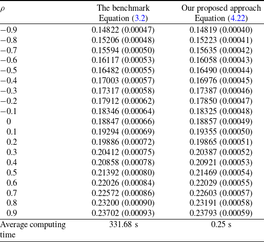
Whilst our approach demonstrates significant efficiency gains over the standard Monte Carlo benchmark, other advanced Monte Carlo techniques exist that further accelerate convergence. Methods such as Quasi-Monte Carlo, which uses deterministic low-discrepancy sequences to improve sampling, and Multilevel Monte Carlo, which allocates computational effort across resolutions, could reduce the number of paths required for a given accuracy by lowering variance. These techniques are complementary to our contribution: whereas they focus on improving sampling efficiency, our change of numéraire technique simplifies the expectation expression itself by eliminating key sources of randomness, specifically, the interest and mortality discount factors, through measure transformation. By adopting the endowment-risk-adjusted measure, we derive a more tractable process that reduces per-path computational complexity. Combining our approach with these advanced sampling methods could yield synergistic gains, a promising direction for future research. Moreover, in industrial applications, large-scale risk and pricing systems often rely on hardware acceleration (e.g., GPU computing) and distributed architectures. The efficiency improvement of our algorithm on a single CPU core suggests strong scaling potential in parallel computing environments, where reduced path complexity and enhanced sampling techniques may be utilised simultaneously.
GMIB value at time $t=0$
with Benefit Base II.
$t=0$
with Benefit Base II.
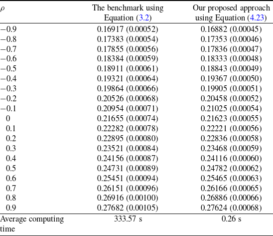
Other observations worthy of note are in regard to the fluctuations of the GMIB value in response to the correlation $\rho$
between interest and mortality rates going from negative to positive, as shown in Figure 1. We have well-reasoned findings with the following considerations: (i) A negative correlation between interest and mortality rates indicates that rising interest rates correspond to declining mortality rates. This diminishes the longevity risk associated with the GMIB, as lower mortality rates imply longer life expectancy for policyholders and greater potential payouts for the insurance company. As a result, the value of the GMIB might increase due to heightened longevity risk, requiring a larger reserve to address future liabilities. (ii) Rising interest rates reduce the present value of forthcoming liabilities. Under a negative interest-mortality correlation, rising interest rates coincide with declining mortality rates. When the impact of reduced mortality dominates the discounting effect of higher interest rates, the net increase in longevity-driven liabilities calls for supplementary reserves to cover extended annuity payout durations. This reserve pressure elevates the GMIB value as insurers have to price the amplified longevity exposure embedded in annuity conversions. (iii) A transition from a negative to a positive correlation may necessitate higher capital reserves to maintain solvency levels, particularly if the risk exposure of the GMIB intensifies. This regulatory imperative to uphold solvency standards could induce an upward surge in the GMIB value. (iv) At
$\rho$
between interest and mortality rates going from negative to positive, as shown in Figure 1. We have well-reasoned findings with the following considerations: (i) A negative correlation between interest and mortality rates indicates that rising interest rates correspond to declining mortality rates. This diminishes the longevity risk associated with the GMIB, as lower mortality rates imply longer life expectancy for policyholders and greater potential payouts for the insurance company. As a result, the value of the GMIB might increase due to heightened longevity risk, requiring a larger reserve to address future liabilities. (ii) Rising interest rates reduce the present value of forthcoming liabilities. Under a negative interest-mortality correlation, rising interest rates coincide with declining mortality rates. When the impact of reduced mortality dominates the discounting effect of higher interest rates, the net increase in longevity-driven liabilities calls for supplementary reserves to cover extended annuity payout durations. This reserve pressure elevates the GMIB value as insurers have to price the amplified longevity exposure embedded in annuity conversions. (iii) A transition from a negative to a positive correlation may necessitate higher capital reserves to maintain solvency levels, particularly if the risk exposure of the GMIB intensifies. This regulatory imperative to uphold solvency standards could induce an upward surge in the GMIB value. (iv) At $\rho = 0$
, the GMIB values are intermediate, but negative correlations (e.g.,
$\rho = 0$
, the GMIB values are intermediate, but negative correlations (e.g., $\rho = -0.5$
) result in a reduction of
$\rho = -0.5$
) result in a reduction of $P_{\text{GMIB}}$
by approximately 15%, whereas positive correlations (e.g.,
$P_{\text{GMIB}}$
by approximately 15%, whereas positive correlations (e.g., $\rho = 0.5$
) increase it by a similar magnitude. Therefore, neglecting dependence structures of mortality and interest rates may induce significant mispricing. (v) Across all values of
$\rho = 0.5$
) increase it by a similar magnitude. Therefore, neglecting dependence structures of mortality and interest rates may induce significant mispricing. (v) Across all values of $\rho$
, Benefit Base II consistently exceeds Benefit Base I in impact to the GMIB value due to its more favourable terms for annuity conversion (e.g., higher income guarantees or more generous crediting rules). These features enhance its value to policyholders, requiring insurers to account for greater liabilities, thereby resulting in a higher GMIB valuation. The persistent gap confirms that whilst
$\rho$
, Benefit Base II consistently exceeds Benefit Base I in impact to the GMIB value due to its more favourable terms for annuity conversion (e.g., higher income guarantees or more generous crediting rules). These features enhance its value to policyholders, requiring insurers to account for greater liabilities, thereby resulting in a higher GMIB valuation. The persistent gap confirms that whilst $\rho$
influences co-movement sensitivity, the baseline valuation is primarily determined by the inherent benefit base’s more liberal design.
$\rho$
influences co-movement sensitivity, the baseline valuation is primarily determined by the inherent benefit base’s more liberal design.
GMIB value at $t=0$
as a function of
$t=0$
as a function of $\rho$
.
$\rho$
.

To further ground our findings in empirical reality, we incorporate market-calibrated estimates from Li et al. (Reference Li, Liu, Tang and Yuan2023). Their analysis of U.S. data (2017–2022) yields an instantaneous correlation between interest rates and excess mortality of $\rho = -0.322$
when including periods of major mortality shocks. Restricting the data to the pre-pandemic period (2017–2019) gives a calibrated correlation of
$\rho = -0.322$
when including periods of major mortality shocks. Restricting the data to the pre-pandemic period (2017–2019) gives a calibrated correlation of $\rho = -0.153$
. Implementing these empirical values in our model generates a material reduction in GMIB value of approximately 4.16% to 8.49% for both benefit bases compared to the independence benchmark (
$\rho = -0.153$
. Implementing these empirical values in our model generates a material reduction in GMIB value of approximately 4.16% to 8.49% for both benefit bases compared to the independence benchmark ( $\rho=0$
). This quantification, derived from real-world parameter estimates, confirms that the impact of mortality-interest rate dependence is a substantive risk phenomenon, not merely a theoretical outcome of parameter sensitivity. Consequently, this empirical evidence reinforces our core conclusion that the interdependence between mortality and interest rates is a meaningful risk factor that should be deliberately incorporated for the accurate valuation of GMIBs.
$\rho=0$
). This quantification, derived from real-world parameter estimates, confirms that the impact of mortality-interest rate dependence is a substantive risk phenomenon, not merely a theoretical outcome of parameter sensitivity. Consequently, this empirical evidence reinforces our core conclusion that the interdependence between mortality and interest rates is a meaningful risk factor that should be deliberately incorporated for the accurate valuation of GMIBs.
5.4. Sensitivity analysis
A sensitivity analysis is conducted to investigate the relationship between the GMIB value and various model parameters. Specifically, we display the GMIB value at $t=0$
as a function of individual model parameters, and the results are exhibited in Figures 2–9. For clarity and ease of interpretation, all the plots in this subsection are generated assuming the Benefit Base II and the correlation coefficient
$t=0$
as a function of individual model parameters, and the results are exhibited in Figures 2–9. For clarity and ease of interpretation, all the plots in this subsection are generated assuming the Benefit Base II and the correlation coefficient $\rho=0$
, unless indicated otherwise.
$\rho=0$
, unless indicated otherwise.
GMIB value at time $t=0$
as a function of
$t=0$
as a function of $\theta$
and
$\theta$
and $\sigma_1$
.
$\sigma_1$
.
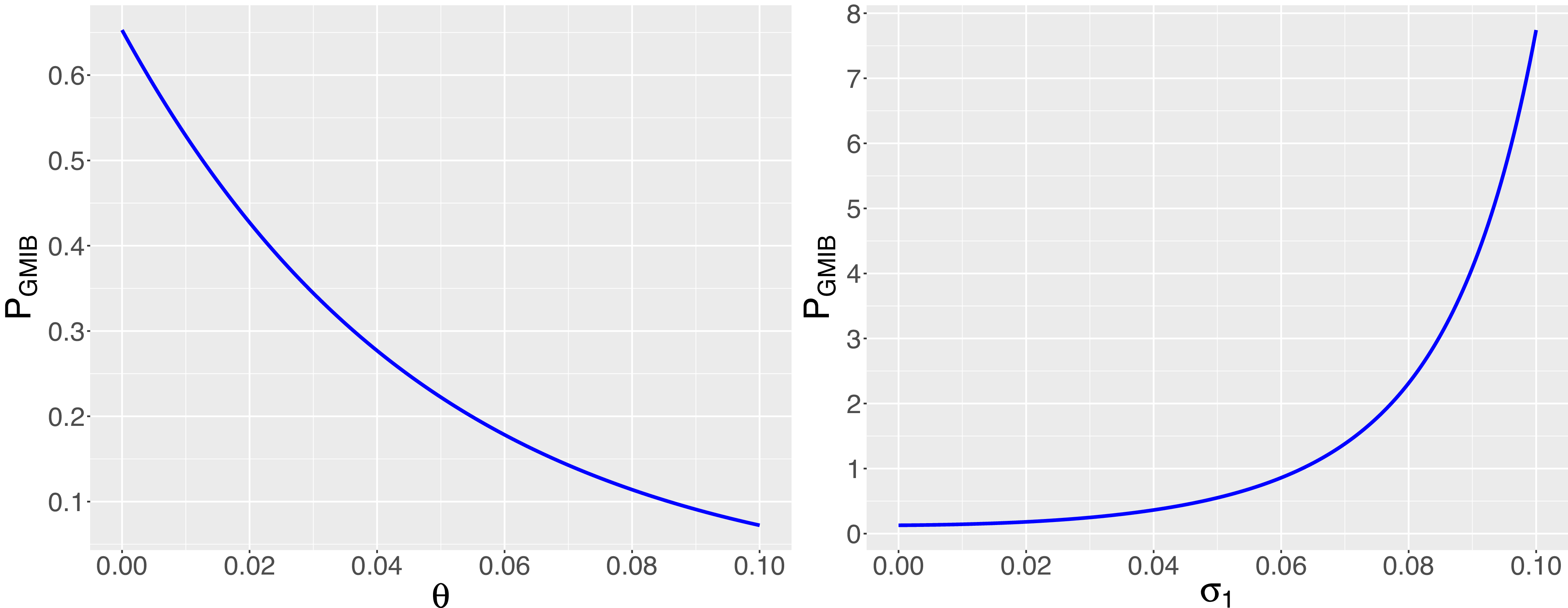
In Figure 2, the GMIB value at $t=0$
is depicted as a function of the parameters in the interest rate model. The left panel illustrates the monotonically decreasing nature of the GMIB value with respect to
$t=0$
is depicted as a function of the parameters in the interest rate model. The left panel illustrates the monotonically decreasing nature of the GMIB value with respect to $\theta$
. This observation is intuitive, as
$\theta$
. This observation is intuitive, as $\theta$
represents the mean-reverting level of the interest rate model. In contrast, the right panel demonstrates that the GMIB value exhibits a monotonically increasing behaviour with the interest rate volatility
$\theta$
represents the mean-reverting level of the interest rate model. In contrast, the right panel demonstrates that the GMIB value exhibits a monotonically increasing behaviour with the interest rate volatility $\sigma_1$
. It is important to note that higher volatility leads to increased variability in both the discounting factor and the annuity factor, necessitating a corresponding increase in the GMIB value to maintain the same return level.
$\sigma_1$
. It is important to note that higher volatility leads to increased variability in both the discounting factor and the annuity factor, necessitating a corresponding increase in the GMIB value to maintain the same return level.
Figure 3 presents the relationship between the GMIB value and the parameter values in the mortality model. The upper two subplots reveal a negative relationship between the GMIB value and the parameters p and h. The parameter p signifies the baseline mortality of the Gompertz function, whilst h represents the associated senescent component. Increasing these parameters effectively raises the mean-reverting level of the mortality rate model, thereby having a higher path in the evolution of the mortality rate. Consequently, the GMIB value is impacted as it is contingent on the survival of the policyholder. A higher mortality rate reduces the likelihood of the policyholder surviving until maturity, diminishing the insurer’s obligation at maturity and subsequently reducing the GMIB value. Moreover, an elevated mortality rate directly diminishes the annuity factor, scaling down the GMIB payoff, resulting in a reduced GMIB value. Additionally, it is observed that the GMIB value increases with a rise in the mortality rate’s volatility $\sigma_2$
. This could be explained by the notion that greater uncertainties in mortality risk make the guaranteed minimum level of annuity payments more enticing upon maturity, consequently leading to a higher GMIB value.
$\sigma_2$
. This could be explained by the notion that greater uncertainties in mortality risk make the guaranteed minimum level of annuity payments more enticing upon maturity, consequently leading to a higher GMIB value.
GMIB value at time $t=0$
as a function of p, h and
$t=0$
as a function of p, h and $\sigma_2$
.
$\sigma_2$
.

In Figure 4, we investigate the sensitivity of the GMIB value at $t=0$
with respect to the volatility
$t=0$
with respect to the volatility $\sigma_3$
of the policyholder’s fund. As anticipated, the GMIB value exhibits a monotonically increasing relationship with
$\sigma_3$
of the policyholder’s fund. As anticipated, the GMIB value exhibits a monotonically increasing relationship with $\sigma_3$
. Higher volatility means increased uncertainty in both the policyholder’s fund account
$\sigma_3$
. Higher volatility means increased uncertainty in both the policyholder’s fund account $F_T$
and the Benefit Base
$F_T$
and the Benefit Base $BB_T$
, consequently leading to a rise in the GMIB value. Moreover, our analysis shows that as
$BB_T$
, consequently leading to a rise in the GMIB value. Moreover, our analysis shows that as $\sigma_3$
goes higher, the discrepancy between the GMIB value with Benefit Base I and the GMIB value with Benefit Base II widens, highlighting the attractiveness of the supplementary discrete lookback feature associated with Benefit Base II.
$\sigma_3$
goes higher, the discrepancy between the GMIB value with Benefit Base I and the GMIB value with Benefit Base II widens, highlighting the attractiveness of the supplementary discrete lookback feature associated with Benefit Base II.
GMIB value at $t=0$
as a function of
$t=0$
as a function of $\sigma_3$
.
$\sigma_3$
.

Figure 5 illustrates the sensitivity of the GMIB value at $t=0$
to the roll-up rate
$t=0$
to the roll-up rate $\delta$
and the guaranteed annuitisation rate g. The left panel displays a positive correlation between the GMIB value and the roll-up rate
$\delta$
and the guaranteed annuitisation rate g. The left panel displays a positive correlation between the GMIB value and the roll-up rate $\delta$
. This relationship is intuitive, as a higher roll-up rate
$\delta$
. This relationship is intuitive, as a higher roll-up rate $\delta$
enhances the Benefit Base, prompting the insurer to offer a greater annual income to the policyholder and hence raising the GMIB value. Conversely, the right panel illustrates a monotonically increasing trend in the GMIB value with the guaranteed annuitisation rate g. A bigger guaranteed annuitisation rate leads to the conversion of the Benefit Base into an annuity with a higher annual payment, thereby boosting the GMIB value.
$\delta$
enhances the Benefit Base, prompting the insurer to offer a greater annual income to the policyholder and hence raising the GMIB value. Conversely, the right panel illustrates a monotonically increasing trend in the GMIB value with the guaranteed annuitisation rate g. A bigger guaranteed annuitisation rate leads to the conversion of the Benefit Base into an annuity with a higher annual payment, thereby boosting the GMIB value.
GMIB value at time $t=0$
as a function of
$t=0$
as a function of $\delta$
and g.
$\delta$
and g.

We examine the relationship between the GMIB value at $t=0$
and its maturity T, as illustrated in Figure 6. Our result reveals an inverted-U shape, telling us that the GMIB value initially increases with maturity, reaches a peak, and subsequently decreases. We note that this pattern arises due to the opposing factors that impact the GMIB value as maturity increases. Specifically, four key factors are observed to influence the GMIB value: (i) the roll-up feature
$t=0$
and its maturity T, as illustrated in Figure 6. Our result reveals an inverted-U shape, telling us that the GMIB value initially increases with maturity, reaches a peak, and subsequently decreases. We note that this pattern arises due to the opposing factors that impact the GMIB value as maturity increases. Specifically, four key factors are observed to influence the GMIB value: (i) the roll-up feature $P_0e^{\delta T}$
in the Benefit Base, which increases the GMIB value over time; (i) the lookback feature
$P_0e^{\delta T}$
in the Benefit Base, which increases the GMIB value over time; (i) the lookback feature $\max \left(F_0,F_5,F_{T} \right)$
in the Benefit Base, which increases the GMIB value due to increased uncertainty in the equity market; (iii) the annuity factor
$\max \left(F_0,F_5,F_{T} \right)$
in the Benefit Base, which increases the GMIB value due to increased uncertainty in the equity market; (iii) the annuity factor $\ddot{a}_{x+T:\overline{n\,}\!\mid}$
, which decreases the GMIB value due to the rising mortality rate after maturity; and (iv) the discounting factor
$\ddot{a}_{x+T:\overline{n\,}\!\mid}$
, which decreases the GMIB value due to the rising mortality rate after maturity; and (iv) the discounting factor $e^{-\int_{0}^{T} r_{u} \mathrm{d}u}e^{-\int_{0}^{T} \mu_{u} \mathrm{d}u}$
, which reduces the GMIB value as it declines. Furthermore, we find that an increase in the roll-up rate
$e^{-\int_{0}^{T} r_{u} \mathrm{d}u}e^{-\int_{0}^{T} \mu_{u} \mathrm{d}u}$
, which reduces the GMIB value as it declines. Furthermore, we find that an increase in the roll-up rate $\delta$
from 0.04 to 0.08 shifts the peak of the GMIB value from
$\delta$
from 0.04 to 0.08 shifts the peak of the GMIB value from $T=15$
to
$T=15$
to $T=20$
.
$T=20$
.
GMIB value at $t=0$
across various maturities T.
$t=0$
across various maturities T.

As well, we analyse in Figure 7 the effects of the risk factors, namely $r_0$
and
$r_0$
and $\mu_0$
, on how the GMIB value varies at time
$\mu_0$
, on how the GMIB value varies at time $t=0$
. The plot discloses that increases in
$t=0$
. The plot discloses that increases in $r_0$
and
$r_0$
and $\mu_0$
correspond to a reduction in the GMIB value. Specifically, within the range of
$\mu_0$
correspond to a reduction in the GMIB value. Specifically, within the range of $-$
30% to 30% adjustments in these risk factors, the GMIB value fluctuates from approximately 14% to
$-$
30% to 30% adjustments in these risk factors, the GMIB value fluctuates from approximately 14% to $-13$
% and from 0.5% to
$-13$
% and from 0.5% to $-0.5$
%, respectively. Consequently, it is evident that the interest rate has a more pronounced impact on the GMIB value compared to the mortality rate. This result is consistent with the fact that as the interest rate impacts both the discount and annuity factors. The mortality rate seems to have a negligible influence. This could be attributed to the still relatively low mortality level of an individual aged 50 at
$-0.5$
%, respectively. Consequently, it is evident that the interest rate has a more pronounced impact on the GMIB value compared to the mortality rate. This result is consistent with the fact that as the interest rate impacts both the discount and annuity factors. The mortality rate seems to have a negligible influence. This could be attributed to the still relatively low mortality level of an individual aged 50 at $t=0$
; thus, a 30% change in mortality renders insignificant change in the GMIB value.
$t=0$
; thus, a 30% change in mortality renders insignificant change in the GMIB value.
Changes in GMIB value at $t=0$
under changes in values of
$t=0$
under changes in values of $r_0$
and
$r_0$
and $\mu_0$
.
$\mu_0$
.

Likewise, we explore the impact of the shifts in the guaranteed annuitisation rate g, roll-up rate $\delta$
, and the volatility of the investment fund
$\delta$
, and the volatility of the investment fund $\sigma_3$
on the GMIB value at
$\sigma_3$
on the GMIB value at $t=0$
, as displayed in Figure 8. We find that an increase in g,
$t=0$
, as displayed in Figure 8. We find that an increase in g, $\sigma_3$
and
$\sigma_3$
and $\delta$
results in a GMIB value rising. More specifically, within the range of
$\delta$
results in a GMIB value rising. More specifically, within the range of $-$
30% to 30% adjustments in these parameters, the GMIB value fluctuates approximately from
$-$
30% to 30% adjustments in these parameters, the GMIB value fluctuates approximately from $-$
52% to 70%, from
$-$
52% to 70%, from $-$
33% to 37%, and from
$-$
33% to 37%, and from $-$
12% to 14%, respectively. More specifically, the guaranteed annuitisation rate g exhibits the most significant impact on the GMIB value. This necessitates insurers to prudently set the guaranteed annuitisation rate at the contract’s inception. In addition, the volatility of the investment fund,
$-$
12% to 14%, respectively. More specifically, the guaranteed annuitisation rate g exhibits the most significant impact on the GMIB value. This necessitates insurers to prudently set the guaranteed annuitisation rate at the contract’s inception. In addition, the volatility of the investment fund, $\sigma_3$
, also carries a considerable influence on the GMIB value. In practical terms, policyholders are typically presented with a selection of investment funds featuring distinct investment strategies and risk profiles at the contract’s commencement. Based on the insights from this analysis, it is advisable for policyholders to select the investment fund with the highest level of volatility when faced with multiple investment fund options that offer identical returns at the same price, thereby maximising the potential for their GMIB value.
$\sigma_3$
, also carries a considerable influence on the GMIB value. In practical terms, policyholders are typically presented with a selection of investment funds featuring distinct investment strategies and risk profiles at the contract’s commencement. Based on the insights from this analysis, it is advisable for policyholders to select the investment fund with the highest level of volatility when faced with multiple investment fund options that offer identical returns at the same price, thereby maximising the potential for their GMIB value.
Variation in the GMIB value at $t=0$
with respect to changes in g,
$t=0$
with respect to changes in g, $\sigma_3$
and
$\sigma_3$
and $\delta$
.
$\delta$
.

Market annuitisation rate $g_{\rm{\scriptsize market}}$
at time
$g_{\rm{\scriptsize market}}$
at time $t=T$
as a function of
$t=T$
as a function of $r_T$
and
$r_T$
and $\mu_T$
.
$\mu_T$
.

As previously discussed, the valuation of the GMIB is intricately sensitive to fluctuations in the guaranteed annuitisation rate g due to the direct impact of g on the potential future payouts under the GMIB rider. When g is more favourable than the prevailing market annuitisation rates at maturity, the policyholder could opt to convert a specified minimum amount of funds into a life annuity at the guaranteed rate at maturity. This advantageous scenario results in higher expected payouts for the insurance company, increasing the value of the GMIB. This bolsters the insurer’s competitive standing and attractiveness to prospective policyholders. However, if g is set excessively high, the insurer will have to correspondingly allocate increased annuity payments. This, in turn, increases reserve requirements and hence exacerbates the financial pressures on the insurer, thereby posing significant challenges to its solvency and liquidity management.
Conversely, if the prevailing market annuitisation rates at maturity surpass g, prospective policyholders may choose to decline the GMIB rider and seek alternative annuitisation options with more favourable market rates from competing insurers. Existing policyholders, on the other hand, might opt to forego the GMIB rider and withdraw their funds to annuitise at a more lucrative market rate. Consequently, the value of the GMIB would diminish as both prospective and current policyholders select better annuitisation avenues outside the GMIB framework. Optimally aligning the guaranteed annuitisation rate with prevailing market annuitisation rates at maturity is vital for preserving the competitiveness and appeal of the GMIB value to policyholders. By calibrating g in consonance with market expectations and prudently managing associated risks, insurers could navigate the delicate balance between offering enticing annuity options to policyholders and upholding financial viability and competitiveness in the marketplace. Such a strategic approach concomitantly enables policyholders to secure a reliable income stream and insurance company to manage their liabilities effectively.
It should be noted that the annuity factor $\ddot{a}_{x+T:\overline{n\,}\!\mid}$
is defined under the risk-neutral measure Q. Therefore, it is the market price of the annuity at the maturity T. Consequently, the market annuitisation rate at the maturity T could be calculated by
$\ddot{a}_{x+T:\overline{n\,}\!\mid}$
is defined under the risk-neutral measure Q. Therefore, it is the market price of the annuity at the maturity T. Consequently, the market annuitisation rate at the maturity T could be calculated by
 \begin{equation*}g_{\rm{\scriptsize market}}=\frac{1}{\ddot{a}_{x+T:\overline{n\,}\!\mid}}=\frac{1}{\sum_{k=0}^{n-1} e^{-\left( A(T,T+k)r_{T} +\widetilde{G}(T,T+k)\mu_{T}\right)+D(T,T+k)+\widetilde{H}(T,T+k)} }.\end{equation*}
In Figure 9, market annuitization rate, we display the time $t=T$
market annuitisation rate
$t=T$
market annuitisation rate $g_{\rm{\scriptsize market}}$
as a function of
$g_{\rm{\scriptsize market}}$
as a function of $r_T$
and
$r_T$
and $\mu_T$
, which could be used by the insurer to determine a fair guaranteed annuitisation rate at the contract’s inception.
$\mu_T$
, which could be used by the insurer to determine a fair guaranteed annuitisation rate at the contract’s inception.
5.5. Impact of mortality risk
Marshall et al. (Reference Marshall, Hardy and Saunders2010) examined the valuation of GMIB in a complete market setting, where mortality was not factored into their valuation framework. In contrast, our study expands upon their model by introducing mortality risk into the analysis. This provides beneficial insights concerning the effect of mortality rates’ fluctuations on the GMIB value across the various annuity terms.
Figure 10, illustrates the GMIB value, where the valuation with mortality risk is compared with the valuation without mortality risk across varying annuity terms n. The valuation of the GMIB is conducted at time $t=0$
with the selection of Benefit Base II. The recalibration of the GMIB in the absence of mortality risk was performed, and the comprehensive details are given in Appendix B. The graphical representation shows an appreciable decline in the GMIB value when mortality risk is embedded in the valuation. For instance, for an annuity term of
$t=0$
with the selection of Benefit Base II. The recalibration of the GMIB in the absence of mortality risk was performed, and the comprehensive details are given in Appendix B. The graphical representation shows an appreciable decline in the GMIB value when mortality risk is embedded in the valuation. For instance, for an annuity term of $n=20$
, the GMIB value with mortality risk amounts to 55.04% of the GMIB value without mortality risk. Notably, the GMIB value reaches a plateau after
$n=20$
, the GMIB value with mortality risk amounts to 55.04% of the GMIB value without mortality risk. Notably, the GMIB value reaches a plateau after $n=30$
, attributed to the rapid increase in mortality rates post age 90 with the inclusion of mortality risk. This plateau implies diminishing marginal liability for insurers as extreme longevity probabilities decay exponentially. In practice, this lends support to converting term annuities into whole-life products, a strategic approach that maintains policyholder appeal whilst containing reserving costs. Crucially, the absence of mortality risk flattens this plateau pattern, as fixed survival assumptions artificially stabilise expected payment duration. By contrast, stochastic mortality modelling accentuates the contraction in actuarial present value beyond age 90, amplifying the term sensitivity. These results demonstrate how mortality risk nonlinearly affects liability exposure through age-dependent mortality acceleration, and must be incorporated explicitly in valuation frameworks to ensure adequate reserving for longevity tail risks.
$n=30$
, attributed to the rapid increase in mortality rates post age 90 with the inclusion of mortality risk. This plateau implies diminishing marginal liability for insurers as extreme longevity probabilities decay exponentially. In practice, this lends support to converting term annuities into whole-life products, a strategic approach that maintains policyholder appeal whilst containing reserving costs. Crucially, the absence of mortality risk flattens this plateau pattern, as fixed survival assumptions artificially stabilise expected payment duration. By contrast, stochastic mortality modelling accentuates the contraction in actuarial present value beyond age 90, amplifying the term sensitivity. These results demonstrate how mortality risk nonlinearly affects liability exposure through age-dependent mortality acceleration, and must be incorporated explicitly in valuation frameworks to ensure adequate reserving for longevity tail risks.
GMIB value with mortality risk versus GMIB value without mortality risk.

5.6. Impact of equity-interest rate correlation
To assess the impact of relaxing the baseline independence assumption in Section 2.3, we investigate the effect of the equity-interest rate correlation ( $\rho^*$
) by conducting a numerical analysis using the same standard Monte Carlo algorithm outlined in Section 5.1. This ensures consistency in computational logic, with the only modification involving the correlation structure via the Cholesky decomposition from Section 2.3. Anchored in empirical evidence, we adopt the market-observed
$\rho^*$
) by conducting a numerical analysis using the same standard Monte Carlo algorithm outlined in Section 5.1. This ensures consistency in computational logic, with the only modification involving the correlation structure via the Cholesky decomposition from Section 2.3. Anchored in empirical evidence, we adopt the market-observed $\rho^*$
values from the calibration of van Haastrecht et al. (Reference van Haastrecht, Plat and Pelsser2010), resulting in interest rate-equity correlations of 0.1464 (U.S.) and 0.3465 (EU). These values serve as plausible benchmarks in our experiments. In addition, we set the mortality-interest rate correlation
$\rho^*$
values from the calibration of van Haastrecht et al. (Reference van Haastrecht, Plat and Pelsser2010), resulting in interest rate-equity correlations of 0.1464 (U.S.) and 0.3465 (EU). These values serve as plausible benchmarks in our experiments. In addition, we set the mortality-interest rate correlation $\rho$
to zero as a control variable to isolate the independent effect of
$\rho$
to zero as a control variable to isolate the independent effect of $\rho^*$
.
$\rho^*$
.
Table 4 presents the GMIB values at time $t=0$
for both Benefit Base I and II under different levels of
$t=0$
for both Benefit Base I and II under different levels of $\rho^*$
, including the baseline case of zero correlation. The results demonstrate a positive relationship between
$\rho^*$
, including the baseline case of zero correlation. The results demonstrate a positive relationship between $\rho^*$
and the GMIB value: as equity returns and interest rates become more positively correlated, the GMIB’s guaranteed income floor becomes more valuable, driven by heightened co-movement risk of market downturns and interest rate fluctuations, which increases policyholders’ demand for downside protection. Specifically, under the U.S.-based market calibration (
$\rho^*$
and the GMIB value: as equity returns and interest rates become more positively correlated, the GMIB’s guaranteed income floor becomes more valuable, driven by heightened co-movement risk of market downturns and interest rate fluctuations, which increases policyholders’ demand for downside protection. Specifically, under the U.S.-based market calibration ( $\rho^* = 0.1464$
), the GMIB value increases by approximately 7.09% and 5.43% for Benefit Base I and II, respectively, relative to the baseline. A more pronounced effect is observed under the EU-based market calibration (
$\rho^* = 0.1464$
), the GMIB value increases by approximately 7.09% and 5.43% for Benefit Base I and II, respectively, relative to the baseline. A more pronounced effect is observed under the EU-based market calibration ( $\rho^* = 0.3465$
), with increases of about 16.24% and 13.38% for the respective benefit bases. Benefit Base II exhibits lower sensitivity to
$\rho^* = 0.3465$
), with increases of about 16.24% and 13.38% for the respective benefit bases. Benefit Base II exhibits lower sensitivity to $\rho^*$
due to its built-in step-up feature (locking in investment gains at policy anniversaries), which reduces reliance on the equity-interest correlation for downside protection, consistent with the design logic of guaranteed minimum benefits.
$\rho^*$
due to its built-in step-up feature (locking in investment gains at policy anniversaries), which reduces reliance on the equity-interest correlation for downside protection, consistent with the design logic of guaranteed minimum benefits.
GMIB value at time $t=0$
under different levels of
$t=0$
under different levels of $\rho^*$
.
$\rho^*$
.
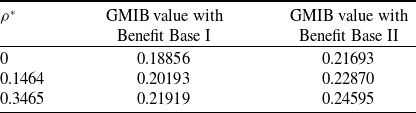
To further evaluate the relative importance of the equity-interest rate dependence, its quantitative impact is compared against that of $\rho$
within a plausible range: an increase in
$\rho$
within a plausible range: an increase in $\rho$
from 0 to 0.4 elevates the GMIB value by approximately 10.95% for Benefit Base I and 11.53% for Benefit Base II. This comparison reveals that the valuation adjustment induced by a realistic
$\rho$
from 0 to 0.4 elevates the GMIB value by approximately 10.95% for Benefit Base I and 11.53% for Benefit Base II. This comparison reveals that the valuation adjustment induced by a realistic $\rho^*$
is comparable in magnitude to that of
$\rho^*$
is comparable in magnitude to that of $\rho$
. The core difference, however, lies not merely in the magnitude of the impact but in the fundamental nature of the risks these correlations represent and their intrinsic relevance to the GMIB product design. The correlation
$\rho$
. The core difference, however, lies not merely in the magnitude of the impact but in the fundamental nature of the risks these correlations represent and their intrinsic relevance to the GMIB product design. The correlation $\rho$
constitutes an endogenous core risk of the product. It directly captures the joint effect of longevity and interest rate risk, the primary exposures that the GMIB is structurally designed to hedge. Its material impact on valuation is an inherent property of the guarantee, and its omission would invalidate the product’s core pricing logic and risk-factor considerations, irrespective of whether its value is set for numerical experimentation or derived empirically. In contrast,
$\rho$
constitutes an endogenous core risk of the product. It directly captures the joint effect of longevity and interest rate risk, the primary exposures that the GMIB is structurally designed to hedge. Its material impact on valuation is an inherent property of the guarantee, and its omission would invalidate the product’s core pricing logic and risk-factor considerations, irrespective of whether its value is set for numerical experimentation or derived empirically. In contrast, $\rho^*$
functions as an exogenous market co-movement risk. Its impact is contingent on specific market regimes (e.g., higher
$\rho^*$
functions as an exogenous market co-movement risk. Its impact is contingent on specific market regimes (e.g., higher $\rho^*$
in the EU market leads to a greater impact) and can be partially offset by policy guarantee mechanisms (e.g., the step-up feature of Benefit Base II) or policyholders’ fund selection, lacking irreplaceability in risk pricing. This analysis validates the rationality of the independence assumption in the baseline model. The potential mispricing introduced by this simplification is quantifiable, contained, and most importantly, does not interfere with the identification and pricing of the product’s core risk drivers.
$\rho^*$
in the EU market leads to a greater impact) and can be partially offset by policy guarantee mechanisms (e.g., the step-up feature of Benefit Base II) or policyholders’ fund selection, lacking irreplaceability in risk pricing. This analysis validates the rationality of the independence assumption in the baseline model. The potential mispricing introduced by this simplification is quantifiable, contained, and most importantly, does not interfere with the identification and pricing of the product’s core risk drivers.
5.7. Impact of lapse risk
In Section 3, it is assumed that the policyholder retains the GMIB until the maturity date of $T=10$
, without incorporating the potential risk of policy lapses into our valuation. The exclusion of lapse risk from our initial model assumption was primarily motivated by the need for tractability in our valuation framework to focus on the core risk factors influencing the GMIB value without introducing additional complexities. However, in the subsequent analysis, we probe the impact of lapse risk on the GMIB value for a more comprehensive assessment of the product’s risk profile. Lapse risk, stemming from the possibly early termination or surrender of the policy by the policyholder, could significantly influence the value and profitability of the GMIB contracts. We aim to see how policy lapses affect the overall value of GMIB and to have a further nuanced understanding of the GMIB’s financial performance and viability.
$T=10$
, without incorporating the potential risk of policy lapses into our valuation. The exclusion of lapse risk from our initial model assumption was primarily motivated by the need for tractability in our valuation framework to focus on the core risk factors influencing the GMIB value without introducing additional complexities. However, in the subsequent analysis, we probe the impact of lapse risk on the GMIB value for a more comprehensive assessment of the product’s risk profile. Lapse risk, stemming from the possibly early termination or surrender of the policy by the policyholder, could significantly influence the value and profitability of the GMIB contracts. We aim to see how policy lapses affect the overall value of GMIB and to have a further nuanced understanding of the GMIB’s financial performance and viability.
The modelling of lapse risk is a challenging task in financial analysis because of lack of data and underdeveloped literature on this area. For the purpose of this study, we opt for a simplified approach by assuming a constant annual lapse rate for ease of computation. Let $P_i$
denote the probability of lapsation within the time period
$P_i$
denote the probability of lapsation within the time period $[i-1,i]$
, corresponding to policy year i where
$[i-1,i]$
, corresponding to policy year i where $i=1,2,\ldots,10$
. Upon lapsation, the policyholder forfeits the right to receive the guaranteed annuitisation rate at maturity, whilst the insurer retains the fees earned from providing the GMIB rider. To account for this lapse risk, we derive the fair value of the lapse-risk-adjusted GMIB at time
$i=1,2,\ldots,10$
. Upon lapsation, the policyholder forfeits the right to receive the guaranteed annuitisation rate at maturity, whilst the insurer retains the fees earned from providing the GMIB rider. To account for this lapse risk, we derive the fair value of the lapse-risk-adjusted GMIB at time $t=0$
as follows:
$t=0$
as follows:
 \begin{align*} P^*_{\rm{\scriptsize GMIB}}(0) =&\, P_1 \cdot 0+ \sum_{i=1}^{T-1} \prod_{j=1}^{i}{(1-P_j)} P_{i+1}\cdot 0 \\&+\prod_{j=1}^{T}(1-P_j) \cdot \mathbb{E}^{Q}\left[e^{-\int_{t}^{T} r_{u} \mathrm{d}u} e^{-\int_{t}^{T} \mu_u \mathrm{d}u}{\max(BB_T g \ddot{a}_{x+T:\overline{n\,}\!\mid} \ -F_{T},0)} \middle |\mathcal{F}_{t}\right] \\[3pt] =&\prod_{j=1}^{T}(1-P_j)P_{\rm{\scriptsize GMIB}}(0),\end{align*}
where $P_{\rm{\scriptsize GMIB}}(0)$
represents the fair value of the GMIB at time
$P_{\rm{\scriptsize GMIB}}(0)$
represents the fair value of the GMIB at time $t=0$
when lapse risk is not considered, that is, the values used in the previous sections.
$t=0$
when lapse risk is not considered, that is, the values used in the previous sections.
Lapse-risk-adjusted GMIB value.

In Table 5, we present the lapse-risk-adjusted GMIB value for various specifications of the lapse rates. The results indicate that incorporating lapse risk has a significant impact on the valuation. For annual lapse rates of 2% and 5%, the lapse-risk-adjusted GMIB value undergoes a notable decrease of 81.71% and 59.87%, respectively, compared to the initial GMIB value. The lapse-risk-adjusted GMIB value diminishes to 69.94% when considering the lapse probabilities for $P_i=5\%$
,
$P_i=5\%$
, $i=1,\ldots,5$
, and
$i=1,\ldots,5$
, and $P_i=2\%$
,
$P_i=2\%$
, $i=6,\ldots,10$
. The magnitude of this decline differs depending on the lapse probability assumptions. Specifically, compared to the scenario where the lapse rate remains constant at 5% throughout the entire contract duration, the decrease in value is less pronounced. In contrast, when considering a lower lapse probability of 2%, the reduction in value is more substantial. In each of the observed scenarios, significant reductions highlight the GMIB valuation’s sensitivity to lapse risk’s fluctuations. Even a minor increase in the lapse risk could lead to significant declines in the GMIB value. This signals that insurers must develop robust methodologies for assessing and managing lapse risk to ensure adequate reserves and capital levels. By recognising and quantifying the influence of lapse risk on GMIB valuation, insurers could shore up workable reserving schemes and risk management frameworks that are more responsive to regulatory capital adequacy mandates.
$i=6,\ldots,10$
. The magnitude of this decline differs depending on the lapse probability assumptions. Specifically, compared to the scenario where the lapse rate remains constant at 5% throughout the entire contract duration, the decrease in value is less pronounced. In contrast, when considering a lower lapse probability of 2%, the reduction in value is more substantial. In each of the observed scenarios, significant reductions highlight the GMIB valuation’s sensitivity to lapse risk’s fluctuations. Even a minor increase in the lapse risk could lead to significant declines in the GMIB value. This signals that insurers must develop robust methodologies for assessing and managing lapse risk to ensure adequate reserves and capital levels. By recognising and quantifying the influence of lapse risk on GMIB valuation, insurers could shore up workable reserving schemes and risk management frameworks that are more responsive to regulatory capital adequacy mandates.
Notably, our model characterises the GMIB rider as a separable contingent claim, independent of the base VA contract. Upon surrender of the VA contract, the policyholder forfeits all rights attached to the GMIB rider, thereby releasing the insurer from any future guarantee obligations. A lapse may occur when the account value exceeds the guaranteed benefit base, rendering the guarantee out-of-the-money. In such cases, policyholders may opt to terminate the contract to avoid ongoing management fees, though this also entails relinquishing any future guaranteed benefits. When the guarantee is deep out-of-the-money, the insurer’s expected future liability is typically low, whilst the policyholder continues to bear the cost of rider fees. This misalignment creates a rational incentive for the policyholder to lapse. For the insurer, this lapse behaviour presents a critical trade-off whereby the reduction in guarantee liabilities following a lapse may be outweighed by the loss of the present value of future fees, particularly when those fees are substantial.
The policyholder receives the account value, net of applicable surrender charges, and the GMIB rider is immediately voided. From the insurer’s perspective, lapse generates two key economic effects: the retention of all previously accrued rider fees and the removal of future guarantee-related liabilities. Since the GMIB is an optional rider contingent on the persistence of the VA contract, its valuation is highly sensitive to policyholder behaviour. Thus, in scenarios where policyholders lapse, especially when the guarantee is out-of-the-money, the insurer’s long-term risk exposure declines, resulting in a lower valuation of the GMIB rider. This is confirmed by our numerical results in Table 5, which demonstrate that the lapse-adjusted GMIB value is lower than the corresponding value under the no-lapse assumption, in line with the findings of Marshall et al. (Reference Marshall, Hardy and Saunders2010). However, this result is contingent upon the simplifying assumption of a constant lapse rate, which does not capture policyholders’ optimal lapse behaviour driven by the economic trade-off between the guarantee’s value and the cumulative fee costs.
Granting the policyholders greater flexibility to lapse optimally, that is, to terminate the contract based on the moneyness of the guarantee and the burden of fees, increases the standalone value of GMIBs from the policyholder’s perspective. This flexibility enables policyholders to retain the option to benefit from future in-the-money guarantees whilst avoiding fee payments when the guarantee is out-of-the-money. From the insurer’s standpoint, this heightened attractiveness results in higher potential liabilities: optimal lapse behaviour reduces the probability of policy termination when the guarantee is in-the-money but increases lapse rates when out-of-the-money. The net effect is that the fair value of the GMIB under optimal lapse behaviour may exceed that under the constant lapse rate assumption, given that the forfeiture of fee income may outweigh the decrease in guarantee liabilities. As such, our current model, which relies on a time-invariant lapse rate, may underestimate the GMIB’s fair value by neglecting this dynamic, wherein the impact of lapse risk is not uniformly value-reducing but contingent upon the optimality of policyholder behaviour. Future research could therefore explore the integration of state-dependent lapse models to more accurately capture policyholder behaviour.
Whilst our time-invariant lapse rate assumption provides computational tractability and initial insights, empirical studies establish lapse dependencies on interest rates and mortality trends (Kuo et al., Reference Kuo, Tsai and Chen2003 and He, Reference He2011). This simplification is purposely adopted to isolate the mortality-interest dependence. However, incorporating the correlation amongst lapse rates, interest rates, and mortality rates may lead to significant complications. These interdependencies could create compounded effects: for instance, interest-mortality covariance may hasten lapse clustering during periods of economic transition, such as interest rate hikes coinciding with mortality shocks like pandemics; this would introduce nonlinear valuation basis risk and other associated concerns. These complex interactions deserve dedicated future research to explore their implications more thoroughly. Potential research pathways include developing a state-dependent lapse rate function linked to stochastic interest rates and mortality dynamics, with an explicitly modelled lapse-mortality-interest rate covariance structure calibrated from historical lapse data stratified by economic regimes and mortality shocks.
6. Conclusion
This paper puts forward a novel stochastic modelling framework for valuing the GMIB by incorporating a dependence structure between interest rates and mortality rates. To accomplish this, we utilised the change of numéraire technique to derive the closed-form valuation formula for the GMIB. The forward measure is established using the bond price as the relevant numéraire, enabling us to obtain an analytic form of the pure endowment. Using further the pure endowment as the numéraire, we came up with the endowment-risk-adjusted measure and derived a GMIB closed-form solution with various forms of the Benefit Base. We conducted numerical experiments, comparing our theoretical outcomes against those from the selected benchmark, which is the Monte-Carlo simulation method. The numerical findings demonstrate the superior accuracy and efficiency of our proposed approach over the benchmark. Furthermore, our sensitivity analyses, exploring the impact of individual model parameters on the GMIB value, yield invaluable guidance to insurers in their business-decision-making processes.
Despite the substantial insights gained from this research study, there are future possibilities for certain directions that could make more progress in the field of insurance product valuation. For instance, one could strengthen the realism of a mortality model by synthesising age, cohort and period-related effects. Models such as M2, M7 and M8 proposed by Cairns et al. (Reference Cairns, Blake, Dowd, Coughlan, Epstein, Ong and Balevich2009) present viable options for incorporating these additional factors into the mortality model settings. In addition, the investment fund model in our analysis made use only of a constant volatility, which may not be true in describing the financial markets over extended periods. Therefore, a stochastic volatility model becomes imperative for a more accurate representation of the fund market value. Some model candidates are the Heston model (Heston, Reference Heston1993) or the regime-switching paradigms (e.g. Xi and Mamon, Reference Xi and Mamon2014; Jalen and Mamon, Reference Jalen and Mamon2014; Gao et al., Reference Gao, Mamon and Liu2015a,b; Mamon et al., Reference Mamon, Xiong and Zhao2020, amongst others). Moreover, capturing policyholders’ behaviours through lapses and early withdrawals from their fund accounts, via stochastic models and integrating them into the modelling framework could provide a more comprehensive understanding of product dynamics and risk management. This aspect of product development, as demonstrated in Barsotti et al. (Reference Barsotti, Milhaud and Salhi2016) and Bernard et al. (Reference Bernard, MacKay and Muehlbeyer2014), enriches the design and associated valuation of insurance products. Lastly, it will be worthwhile research undertakings to extend the modelling framework and the change of numéraire technique employed in this study to investigate the valuation of other guarantee riders, such as the GMAB (Huang et al., Reference Huang, Mamon and Xiong2022), GMWB (Milevsky and Salisbury, Reference Milevsky and Salisbury2006; Dai et al., Reference Dai, Kuen Kwok and Zong2008; Feng and Jing, Reference Feng and Jing2017, and Fung and Sherris, Reference Fung, Ignatieva and Sherris2014) and equity-indexed annuity (Lin and Tan, Reference Lin and Tan2003 and Tiong, Reference Tiong2000).
Acknowledgements
We would like to extend our sincere thanks to the two anonymous reviewers and the Editor for their valuable comments and suggestions, which have greatly improved the manuscript. The support of the Natural Sciences and Engineering Research Council of Canada, through R. Mamon’s Discovery Grant (RGPIN-2017-04235), and the China State Administration of Foreign Experts Affairs (H20240471), is gratefully acknowledged. H. Xiong expresses his appreciation for the support of the Humanities and Social Sciences Foundation of the Ministry of Education of China (MOE) (23YJCZH001).
Competing interests
The authors declare no competing interests of any kind.
Appendix A. From the real-world measure to the risk-neutral measure
This appendix details the probability-measure change from the real-world measure P to the risk-neutral measure Q. Such a change of measure connects the outcomes obtained within the risk-neutral framework and those within the real-world framework, where empirical data are utilised for model calibration purposes.
Let us assume that the P-dynamics of $r_t$
,
$r_t$
, $\mu_t$
and
$\mu_t$
and $S_t$
are given by
$S_t$
are given by
 \begin{align*}\mathrm{d}r_{t} &= a^{*}(\theta_1^{*}(t)-r_{t})\mathrm{d}t+\sigma_1 \mathrm{d}W_{t}^{1,P}, \\[3pt]\mathrm{d}\mu_{t} &= c^{*}(\xi_1^{*}(t)-\mu_{t})\mathrm{d}t+\sigma_2 \big( \rho\mathrm{d}W_{t}^{1,P}+ \sqrt{1-\rho^{2}}\mathrm{d}W_{t}^{2,P}\big), \, {\text{and}}\\[3pt]\mathrm{d}S_t & = {u_t}{S_t}\mathrm{d}t+\sigma_3S_t\mathrm{d}W_{t}^{3,P},\end{align*}
where $a^*$
,
$a^*$
, $\sigma_1$
,
$\sigma_1$
, $c^*$
,
$c^*$
, $\sigma_2$
and
$\sigma_2$
and $\sigma_3$
are positive constants,
$\sigma_3$
are positive constants, $W_{t}^{1,P}$
,
$W_{t}^{1,P}$
, $W_{t}^{2,P}$
and
$W_{t}^{2,P}$
and $W_{t}^{3,P}$
are independent standard P-BMs.
$W_{t}^{3,P}$
are independent standard P-BMs.
Following the principles adopted by Dahl and Møller (Reference Dahl and Møller2006), we consider a likelihood process $\Lambda_{t}^{P}$
of the form
$\Lambda_{t}^{P}$
of the form
 \begin{align*} \,\, \,\,\,\,\,\,\,\,\,\,\,\!\mathrm{d}\Lambda_{t}^{P} &= -\Lambda_{t}^{P}\left[f_{r}(t)\mathrm{d}W_{t}^{1,P}+f_{\mu}(t)\mathrm{d}W_{t}^{2,P}+f_{S}(t)\mathrm{d}W_{t}^{3,P}\right],\ \ \Lambda_{0}^{P}=1,\end{align*}
where
 \begin{align*}f_{r}(t) &=\frac{c_1 \theta_2^{*}(t)+c_2r_t}{\sigma_1},\\[3pt]f_{\mu}(t) &=\frac{c_3 \sigma_1 \xi_2^{*}(t)-c_1\sigma_2\rho\theta_2^{*}(t)-c_2\sigma_2 \rho r_t+c_4\sigma_1 \mu_t}{\sigma_1 \sigma_2 \sqrt{1-\rho^2}}, \, {\text{and}}\\f_{S}(t) &=\frac{u_t-r_t}{\sigma_2}.\end{align*}
Here, $c_1$
,
$c_1$
, $c_2$
,
$c_2$
, $c_3$
and
$c_3$
and $c_4$
are constants satisfying
$c_4$
are constants satisfying $c_1 \lt 0$
,
$c_1 \lt 0$
, $c_2 \lt -a^*$
,
$c_2 \lt -a^*$
, $c_3 \lt 0$
and
$c_3 \lt 0$
and $c_4 \lt -c^*$
.
$c_4 \lt -c^*$
.
Given that $\mathbb{E}^{P}\left[\Lambda_{T}^{0}\right]=1$
, we establish the risk-neutral measure Q as equivalent to the real-world measure P via the Radon–Nikodým derivative
$\mathbb{E}^{P}\left[\Lambda_{T}^{0}\right]=1$
, we establish the risk-neutral measure Q as equivalent to the real-world measure P via the Radon–Nikodým derivative
 \begin{align*} \left.\frac{\mathrm{d}Q}{\mathrm{d}P} \right|_{\mathcal{F}_{T}}=\Lambda_{T}^{P}. \end{align*}
Invoking the the Girsanov’s Theorem, $W_{t}^{1}$
,
$W_{t}^{1}$
, $W_{t}^{2}$
and
$W_{t}^{2}$
and $W_{t}^{3}$
are standard Q-BMs, where
$W_{t}^{3}$
are standard Q-BMs, where
 \begin{align*}\mathrm{d}W_{t}^{1}&=\mathrm{d}W_{t}^{1,P}+f_{r}(t)\mathrm{d}t,\\[3pt]\mathrm{d}W_{t}^{2}&=\mathrm{d}W_{t}^{2,P}+f_{\mu}(t)\mathrm{d}t, \, {\text{and}}\\[3pt]\mathrm{d}W_{t}^{3}&=\mathrm{d}W_{t}^{3,P}+f_{S}(t)\mathrm{d}t.\end{align*}
The respective Q-dynamics of $r_t$
,
$r_t$
, $\mu_t$
and
$\mu_t$
and $S_t$
are then given by
$S_t$
are then given by
 \begin{align*}\mathrm{d}r_{t} &= a(\theta(t)-r_{t})\mathrm{d}t+\sigma_1 \mathrm{d}W_{t}^{1}, \\[3pt]\mathrm{d}\mu_{t} &= c(\xi(t)-\mu_{t})\mathrm{d}t+\sigma_2 \big(\rho \mathrm{d}W_{t}^{1}+ \sqrt{1-\rho^{2}}\mathrm{d}W_{t}^{2} \big), \, {\text{and}}\\[3pt]\mathrm{d}S_t & = {r_t}{S_t}\mathrm{d}t+{\sigma_3}S_t\mathrm{d}{W_{t}^{3}},\end{align*}
where $a=a^*+c_2$
,
$a=a^*+c_2$
,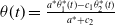 $\theta(t)=\frac{a^* \theta_1^*(t)-c_1\theta_2^*(t)}{a^*+c_2}$
,
$\theta(t)=\frac{a^* \theta_1^*(t)-c_1\theta_2^*(t)}{a^*+c_2}$
, $c=c^*+c_4$
, and
$c=c^*+c_4$
, and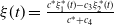 $\xi(t)=\frac{c^* \xi_1^*(t)-c_3\xi_2^*(t)}{c^*+c_4}$
.
$\xi(t)=\frac{c^* \xi_1^*(t)-c_3\xi_2^*(t)}{c^*+c_4}$
.
Appendix B. The evaluation of GMIB in the absence of mortality risk
In this appendix, we derive the value of the GMIB under the modelling framework that incorporates only the interest-rate and investment-fund risks; that is, the valuation is performed in the absence of mortality risk.
Under the measure Q, the dynamics of $r_t$
and
$r_t$
and $F_t$
are given by
$F_t$
are given by
 \begin{align*}\mathrm{d}r_{t}&= a \left[\theta(t)- r_{t}\right]\mathrm{d}t + \sigma_1 \mathrm{d}W_{t}^{1}, \, {\text{and}}\\[3pt]\mathrm{d}F_{t}&= ({r_t}-\alpha){F_t}dt+\sigma_3 F_t \mathrm{d}W_{t}^{3}. \end{align*}
The fair value of the GMIB under the risk-neutral measure is
 \begin{align*}P_{\rm{\scriptsize GMIB}}(t) = \mathbb{E}^{Q}\left[e^{-\int_{t}^{T} r_{u} \mathrm{d}u} {\max(BB_T g \ddot{a}_{\overline{n\,}\!\mid}(T) -F_{T},0)}\middle |\mathcal{F}_{t}\right], \end{align*}
where the annuity factor is an annuity-certain due, with the first payment at time T and could be decomposed into a sum of zero-coupon bonds, that is,
 \begin{equation*}\ddot{a}_{\overline{n\,}\!\mid}(T)=\sum_{k=0}^{n-1}B(T,T+k)=\sum_{k=0}^{n-1} e^{- A(T,T+k)r_{T}+D(T,T+k)}.\end{equation*}
The Benefit Base is given by
 \begin{equation*}BB_T =\begin{cases}P_0e^{\delta T}& \text{Benefit Base I}, \\[3pt]\max{ \left( P_0e^{\delta T}, F_{t_1}, F_{t_1}, \cdots, F_{t_m} \right)}& \text{Benefit Base II}.\end{cases}\end{equation*}
We define the forward measure $\widetilde{Q}$
equivalent to the risk-neutral measure Q via the Radon–Nikodým derivative
$\widetilde{Q}$
equivalent to the risk-neutral measure Q via the Radon–Nikodým derivative
 \begin{align*} \left.\frac{\mathrm{d}\widetilde{Q}}{\mathrm{d}Q}\right|_ {\mathcal{F}_{T}}=\Lambda^{1}_{T}\, :\!=\, \frac{e^{-\int_{0}^{T}r_{u}\mathrm{d}u}B(T,T)}{B(0,T)}. \end{align*}
By the Bayes’ rule for conditional expectations, B
 \begin{align}P_{\rm{\scriptsize GMIB}}(t) &= \mathbb{E}^{Q}\left[e^{-\int_{t}^{T}r_{u}\mathrm{d}u}{\max(BB_T g \ddot{a}_{\overline{n\,}\!\mid}(T) -F_{T},0)}\middle |\mathcal{F}_{t}\right] \nonumber \\&=B(t, T)\mathbb{E}^{\widetilde{Q}}\left[{\max(BB_T g \ddot{a}_{\overline{n\,}\!\mid}(T) -F_{T},0)}\middle |\mathcal{F}_{t}\right]. \end{align}
In order to evaluate the expectation of the payoff in Equation (B1), we need the $\widetilde{Q}$
-dynamics of
$\widetilde{Q}$
-dynamics of $r_t$
and
$r_t$
and $F_T$
.
$F_T$
.
Our calculations show that
 \begin{equation*}\mathrm{d}\Lambda_{t}^{1}=-\sigma_1 A(t,T^*) \Lambda_{t}^{1}\mathrm{d}W_{t}^{1}.\end{equation*}
By the Girsanov’s Theorem, $\widetilde{W}_{t}^{1}$
and
$\widetilde{W}_{t}^{1}$
and $\widetilde{W}_{t}^{3}$
are standard BMs under
$\widetilde{W}_{t}^{3}$
are standard BMs under $\widetilde{Q}$
, where
$\widetilde{Q}$
, where
 \begin{align*}\mathrm{d}\widetilde{W}_{t}^{1} &= \mathrm{d}W_{t}^{1}+\sigma_1 A(t, T)\mathrm{d}t, \, {\text{and}} \\[3pt]\mathrm{d}\widetilde{W}_{t}^{3} &= \mathrm{d}W_{t}^{3}.\end{align*}
Therefore, the $\widetilde{Q}$
dynamics of
$\widetilde{Q}$
dynamics of $r_{t}$
and
$r_{t}$
and $F_{t}$
are given by
$F_{t}$
are given by
 \begin{align}\mathrm{d}r_{t} &= [a\theta(t)-\sigma_1^{2}A(t, T)-ar_{t}]\mathrm{d}t+\sigma_1 \mathrm{d}\widetilde{W}_{t}^{1}, \, {\text{and}} \\[-8pt] \nonumber \end{align}
 \begin{align} \mathrm{d}F_{t} &= ({r_t}-\alpha){F_t}dt+\sigma_3 F_t \mathrm{d}\widetilde{W}_{t}^{3}. \\[6pt] \nonumber\end{align}
Solving Equation (B2), for $u \geq t$
,
$u \geq t$
,
 \begin{align}r_u&=e^{-a(u-t)}r_t + a e^{-au} \int_{t}^{u} e^{as} \theta(s) \mathrm{d}s - \frac{\sigma_1^2}{a^2} \left(1-e^{-a(u-t)} \right) \nonumber \\ &\quad+ \frac{\sigma_1^2 e^{-aT}}{2a^2} (e^{au} - e^{-au+2at}) + \sigma_{1}e^{-au} \int_{t}^{u}e^{as}\mathrm{d}\widehat{W}_{s}^{1}. \end{align}
Integrating Equation (B4), we obtain
 \begin{align}\int_{t}^{t^*} {r_u}\mathrm{d}u&= r_t \frac{1- e^{-a(t^*-t)}}{a} - \frac{\sigma_1^2}{a^2} \left( t^*- t - \frac{1- e^{-a(t^*-t)}}{a} \right) + \frac{\sigma_1^2 e^{-aT}}{2a^2} \left( \frac{e^{at^*} - e^{at}}{a} - \frac{e^{at} - e^{-at^*+2at}}{a}\right) \nonumber \\[3pt]&\quad+ \int_{t}^{t^*} \theta(s) \left( 1- e^{-a(t^*-s)} \right) \mathrm{d}s + \frac{\sigma_{1}}{a} \int_{t}^{t^*} \left( 1- e^{-a(t^*-s)} \right) \mathrm{d}\widehat{W}_{s}^{1}. \end{align}
Solving Equation (B3), for $t^* \geq t$
, we obtain
$t^* \geq t$
, we obtain
 \begin{equation*}F_{t^*}=F_{t}\exp{\left[\int_{t}^{t^*} {\left(r_u-\alpha-\frac{1}{2}\sigma_3^2\right)}\mathrm{d}u + \sigma_3\left(\widehat{W}_{t^*}^{3} - \widehat{W}_{t}^{3}\right)\right]}.\end{equation*}
Write
 \begin{align}Y_{t,\ t^*}\, :\!=\, \int_{t}^{t^*} {\left(r_u-\alpha-\frac{1}{2}\sigma_3^2\right)}\mathrm{d}u + \sigma_3\left(\widehat{W}_{t^*}^{3} - \widehat{W}_{t}^{3}\right)=\int_{t}^{t^*} {r_u}\mathrm{d}u - \left(\alpha+\frac{1}{2}\sigma_3^2\right) (t^* - t) + \sigma_3\left(\widehat{W}_{t^*}^{3} - \widehat{W}_{t}^{3}\right). \end{align}
Combining Equations (B5) and (B6), we have
 \begin{align}Y_{t,\ t^*}&= r_t \frac{1- e^{-a(t^*-t)}}{a} - \frac{\sigma_1^2}{a^2} \left( t^*- t - \frac{1- e^{-a(t^*-t)}}{a} \right) + \frac{\sigma_1^2 e^{-aT}}{2a^2} \left( \frac{e^{at^*} - e^{at}}{a} - \frac{e^{at} - e^{-at^*+2at}}{a}\right) \nonumber \\[3pt]&\quad+ \int_{t}^{t^*} \theta(s) \left( 1- e^{-a(t^*-s)} \right) \mathrm{d}s - \left(\alpha+\frac{1}{2}\sigma_3^2\right) (t^* - t)+\frac{\sigma_1}{a} \int_{t}^{t^*} \left( 1- e^{-a(t^*-s)} \right) \mathrm{d}\widehat{W}_{s}^{1} + \sigma_3\left(\widehat{W}_{t^*}^{3} - \widehat{W}_{t}^{3}\right) . \end{align}
Based on Equations (B4) and (B7), we have the following result.
Theorem B.1. In the absence of mortality risk, the GMIB value, under the Benefit Base I, at time $t \leq T$
is
$t \leq T$
is
 \begin{align} P^{* \ (I)}_{\rm{\scriptsize GMIB}}(t) = e^{- A(t, T)r_{t} +D(t, T)} \mathbb{E}^{\widehat{Q}} \left[\max(g P_0 e^{\delta T} \sum_{k=0}^{n-1} e^{- A(T,T+k)r_{T} +D(T,T+k)} -F_t e^{Y_{t,\ T}},0) \middle |\mathcal{F}_{t}\right], \end{align}
where the conditional distribution of $\{r_T,\ Y_{t,\ T}\}$
given
$\{r_T,\ Y_{t,\ T}\}$
given $\mathcal{F}_t$
follows a bivariate normal distribution characterised by the following parameters:
$\mathcal{F}_t$
follows a bivariate normal distribution characterised by the following parameters:
 \begin{align*} \mathbb{E}^{\widehat{Q}}\left[ r_T \middle| \mathcal{F}_{t}\right]= e^{-a(T-t)}r_t + a e^{-aT} \int_{t}^{T} e^{as} \theta(s) \mathrm{d}s -\frac{\sigma_1^2}{a^2} \left(1-e^{-a(T-t)} \right) + \frac{\sigma_1^2 }{2a^2} \left(1 - e^{-2a(T-t)}\right),\end{align*}
 \begin{align*} \mathbb{E}^{\widehat{Q}}\left[ Y_{t,\ T} \middle| \mathcal{F}_{t}\right]&=r_t \frac{1- e^{-a(T-t)}}{a} +\int_{t}^{T} \theta(s) \left( 1- e^{-a(T-s)} \right) \mathrm{d}s - \frac{\sigma_1^2}{a^2} \left( T- t - \frac{1- e^{-a(T-t)}}{a} \right) \nonumber \\[3pt] &\quad+\frac{\sigma_1^2}{2a^2} \left( \frac{1 - e^{-a(T-t)}}{a} - \frac{e^{-a(T-t)} - e^{-2a(T-t)}}{a}\right) - \left(\alpha+\frac{1}{2}\sigma_3^2\right) (T - t), \nonumber\end{align*}
 \begin{align*} \mathbb{V}{\text{ar}}^{\widehat{Q}}\left[r_T \middle| \mathcal{F}_{t} \right]=\frac{\sigma_1^2}{2a} \big( 1 - e^{-2a(T-t)} \big),\end{align*}
 \begin{align*} \mathbb{V}{\text{ar}}^{\widehat{Q}}[ Y_{t,\ T} | \mathcal{F}_{t} ]=\left( \frac{\sigma_1^2}{a^2}+\sigma_3^2 \right) (T-t) - \frac{2\sigma_1^2}{a^3} \left( 1 - e^{-a(T-t)}\right) + \frac{\sigma_1^2}{2a^3} \left( 1 - e^{-2a(T-t)}\right)\!, \, {{and}}\end{align*}
 \begin{equation*} \mathbb{C}{\text{ov}}^{\widehat{Q}}[r_T, Y_{t,\ T} \big |\mathcal{F}_{t} ]=\frac{\sigma_1^2}{2a^2}\left(1-2e^{-a(T-t)}+e^{-2a(T-t)}\right).\end{equation*}
Theorem B.2. In the absence of mortality risk, the GMIB value, under the Benefit Base II, at time $t \leq T$
is
$t \leq T$
is
 \begin{align} P^{* \ (II)}_{\rm{\scriptsize GMIB}}(t)= & e^{- A(t, T)r_{t} +D(t, T)}\mathbb{E}^{\widehat{Q}} \left[\max\big( g \max{ \big( P_0 e^{\delta T},\max_{i \in \overline{I_t}} F_{t_i},\max_{i \in I_t} F_t e^{Y_{t,\ t_i}} \big) \big. \big.} \right. \nonumber \\ &\left. \sum_{k=0}^{n-1} e^{- A(T,T+k)r_{T} +D(T,T+k)} -F_t e^{Y_{t,\ T}},0 \big. \big) \big | \big. \mathcal{F}_{t} \big. \right], \end{align}
where $r_T, \ Y_{t,\ t_i}, \text{for} \ i \in I_t$
conditional on
$r_T, \ Y_{t,\ t_i}, \text{for} \ i \in I_t$
conditional on $\mathcal{F}_t$
follow a multivariate normal distribution, with the following parameters:
$\mathcal{F}_t$
follow a multivariate normal distribution, with the following parameters:
 \begin{align*}\mathbb{E}^{\widehat{Q}}\left[ r_T \middle| \mathcal{F}_{t}\right]= e^{-a(T-t)}r_t + a e^{-aT} \int_{t}^{T} e^{as} \theta(s) \mathrm{d}s -\frac{\sigma_1^2}{a^2} \left(1-e^{-a(T-t)} \right) + \frac{\sigma_1^2 }{2a^2} \left(1 - e^{-2a(T-t)}\right), \end{align*}
 \begin{align*} \mathbb{E}^{\widehat{Q}}\left[ Y_{t,\ t_i} \middle| \mathcal{F}_{t}\right]&=r_t \frac{1- e^{-a(t_i-t)}}{a} + \int_{t}^{t_i} \theta(s) \left( 1- e^{-a(t_i-s)} \right) \mathrm{d}s - \frac{\sigma_1^2}{a^2} \left( t_i - t - \frac{1- e^{-a(t_i-t)}}{a} \right) \nonumber \\[3pt] &\quad+ \frac{\sigma_1^2e^{-aT}}{2a^2} \left( \frac{e^{at_i} - e^{at} }{a} - \frac{e^{at} - e^{-at_i+2at}}{a} \right) - \left(\alpha+\frac{1}{2}\sigma_3^2\right) (t_i - t), i \in I_t,\end{align*}
 \begin{align*} \mathbb{V}{\text{ar}}^{\widehat{Q}}\left[r_T \middle| \mathcal{F}_{t} \right]=\frac{\sigma_1^2}{2a} \left( 1 - e^{-2a(T-t)} \right)\!,\end{align*}
 \begin{align*} \mathbb{V}{\text{ar}}^{\widehat{Q}}\left[ Y_{t,\ t_i} \middle| \mathcal{F}_{t} \right]=\left( \frac{\sigma_1^2}{a^2}+\sigma_3^2 \right) (t_i-t) - \frac{2\sigma_1^2}{a^3} \left( 1 - e^{-a(t_i-t)}\right) + \frac{\sigma_1^2}{2a^3} \left( 1 - e^{-2a(t_i-t)}\right)\! , i \in I_t,\end{align*}
 \begin{equation*} \mathbb{C}{\text{ov}}^{\widehat{Q}}\left[r_T, Y_{t,\ t_i} \middle |\mathcal{F}_{t} \right]=\frac{\sigma_1^2}{2a^2}\left(e^{-a(T-t_i)}-2e^{-a(T-t)}+e^{-a(T+t_i-2t)}\right)\!, i\in I_t, \, {{and}}\end{equation*}
 \begin{align*} \mathbb{C}{\text{ov}}^{\widehat{Q}}\left[Y_{t,\ t_i}, Y_{t,\ t_j}\middle |\mathcal{F}_{t} \right]&=\left( \frac{\sigma_1^2}{a^2}+\sigma_3^2 \right) (t_i-t) - \frac{\sigma_1^2}{a^3} \left( e^{-at_i} + e^{-at_j}\right) \left(e^{at_i}-e^{at}\right) \\&\quad+ \frac{\sigma_1^2}{2a^3} \left( e^{-a(t_j-t_i)} - e^{-a(t_i+t_j-2t)}\right), i \lt j,\ i,j \in I_t.\end{align*}
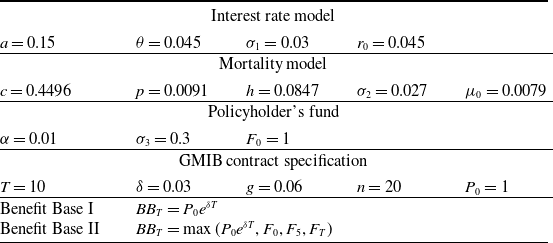
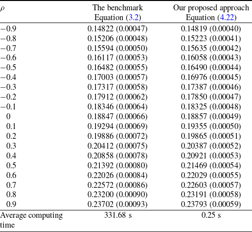

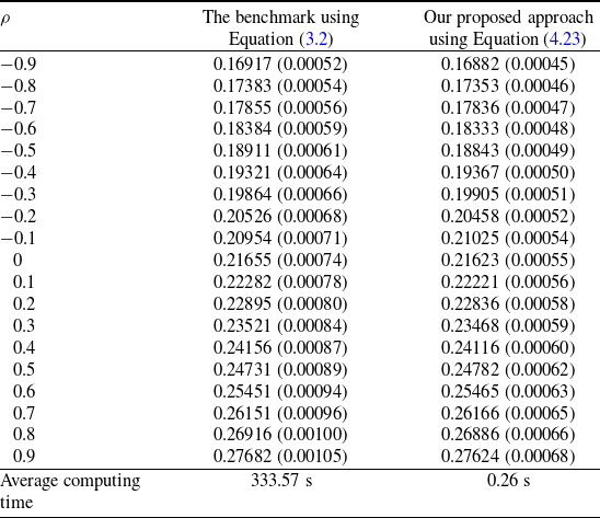

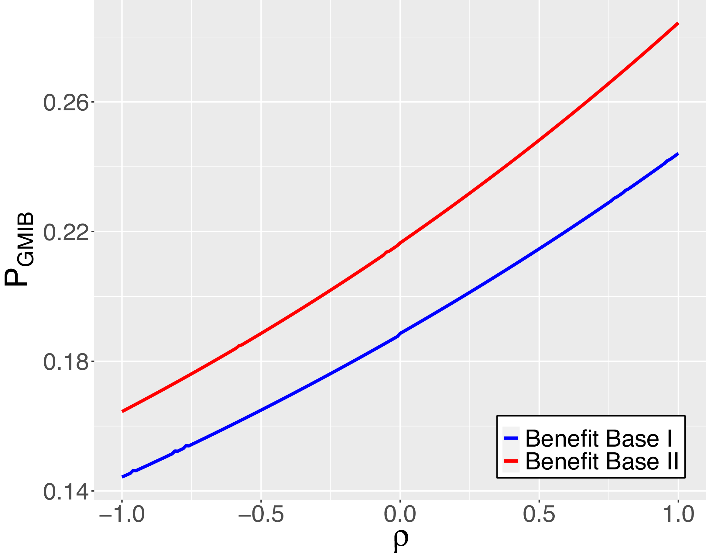


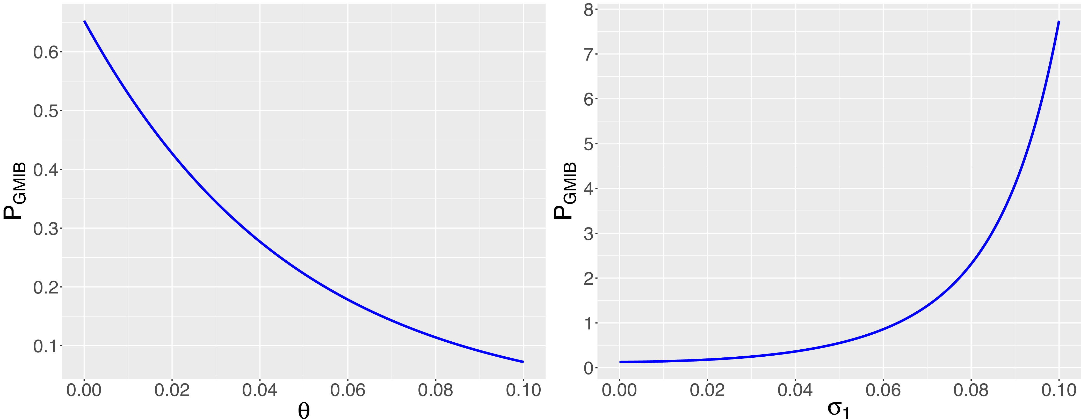


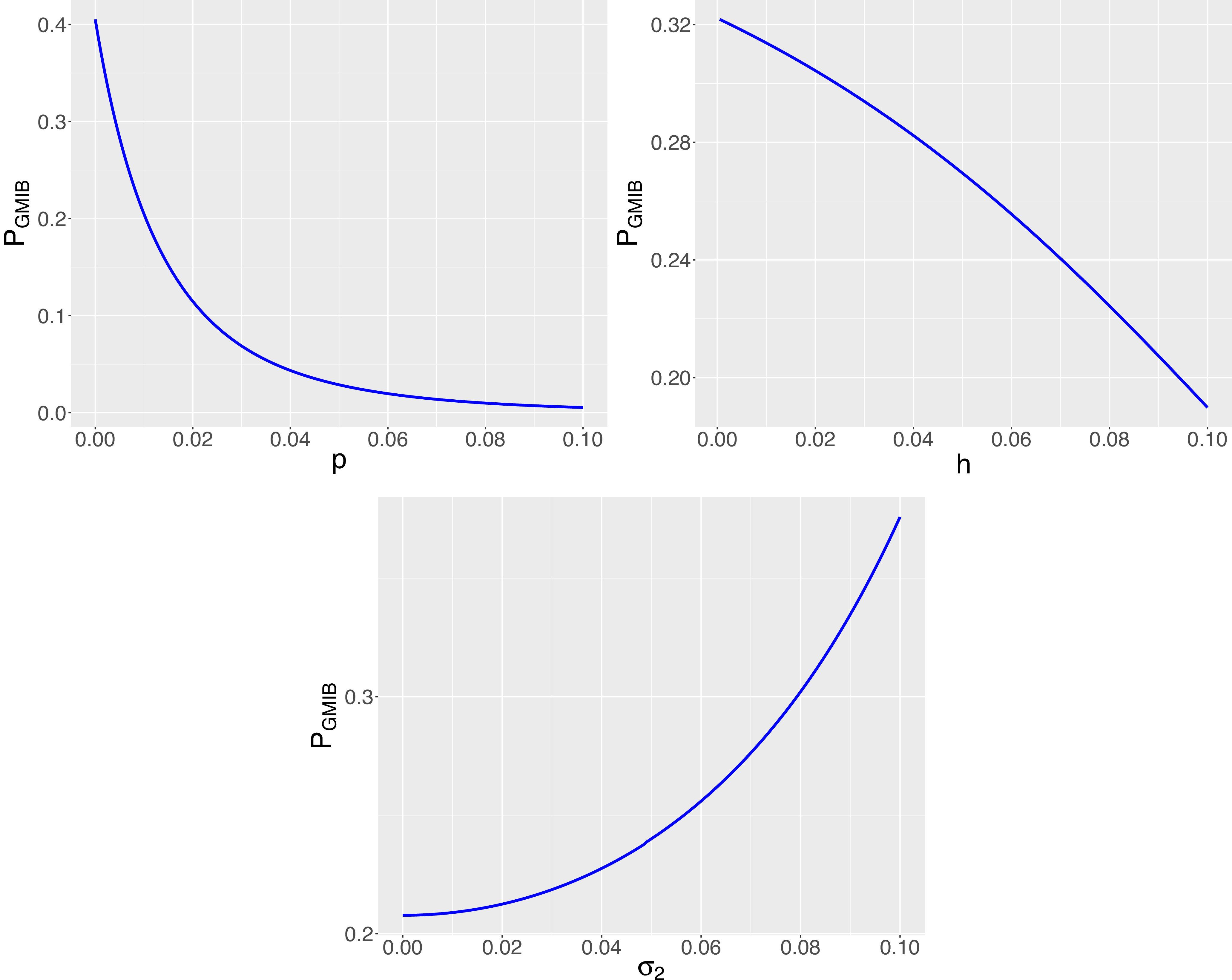


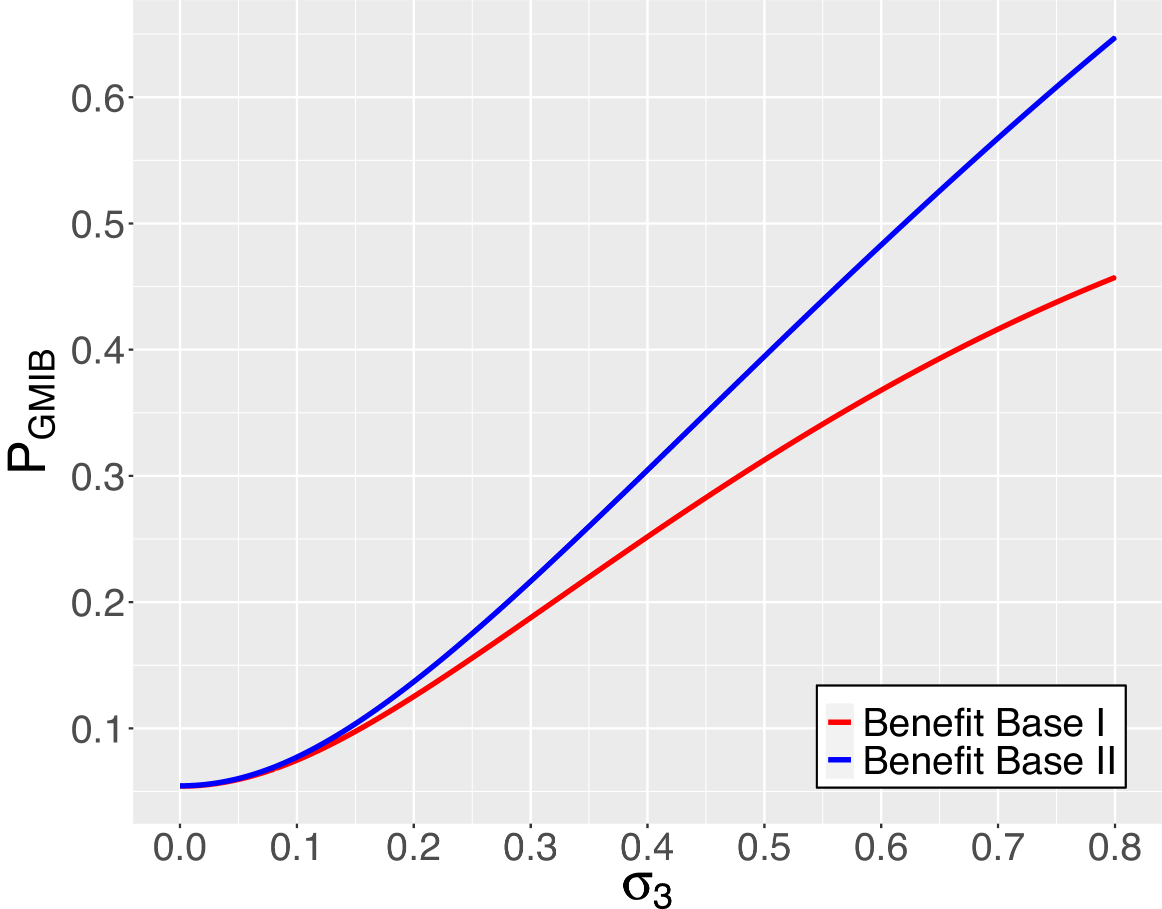


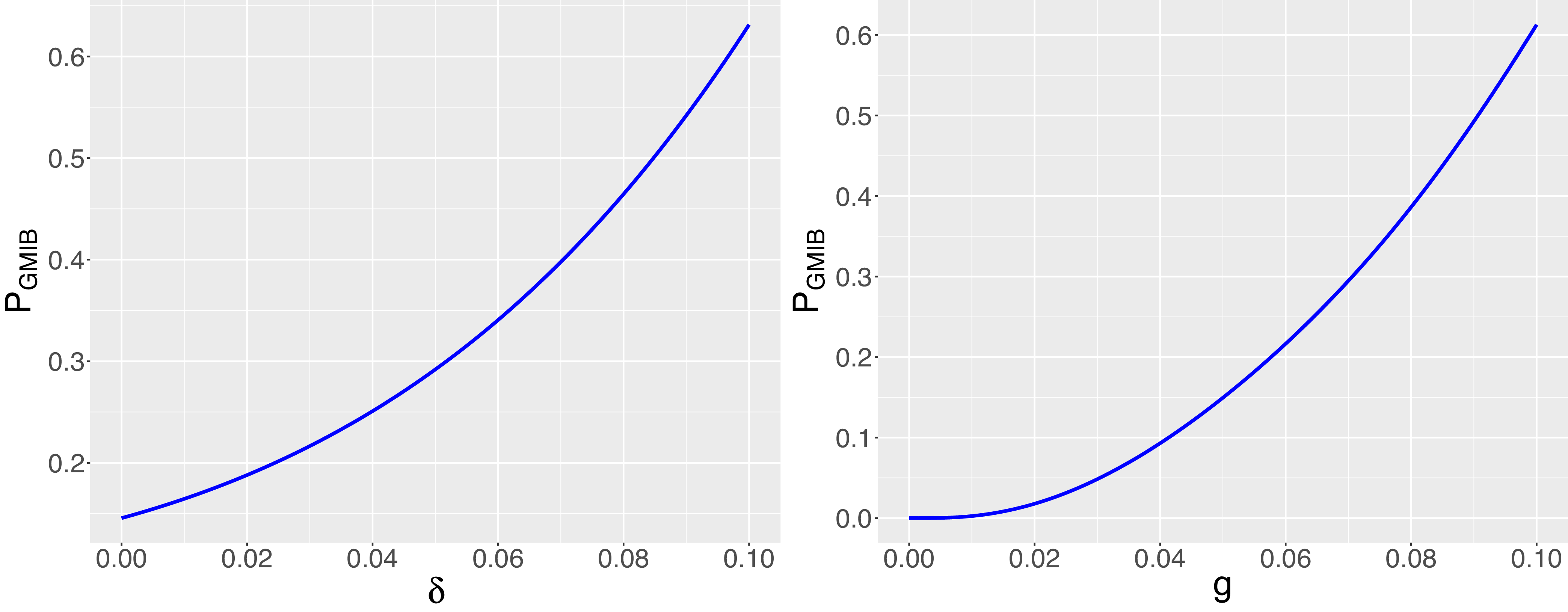


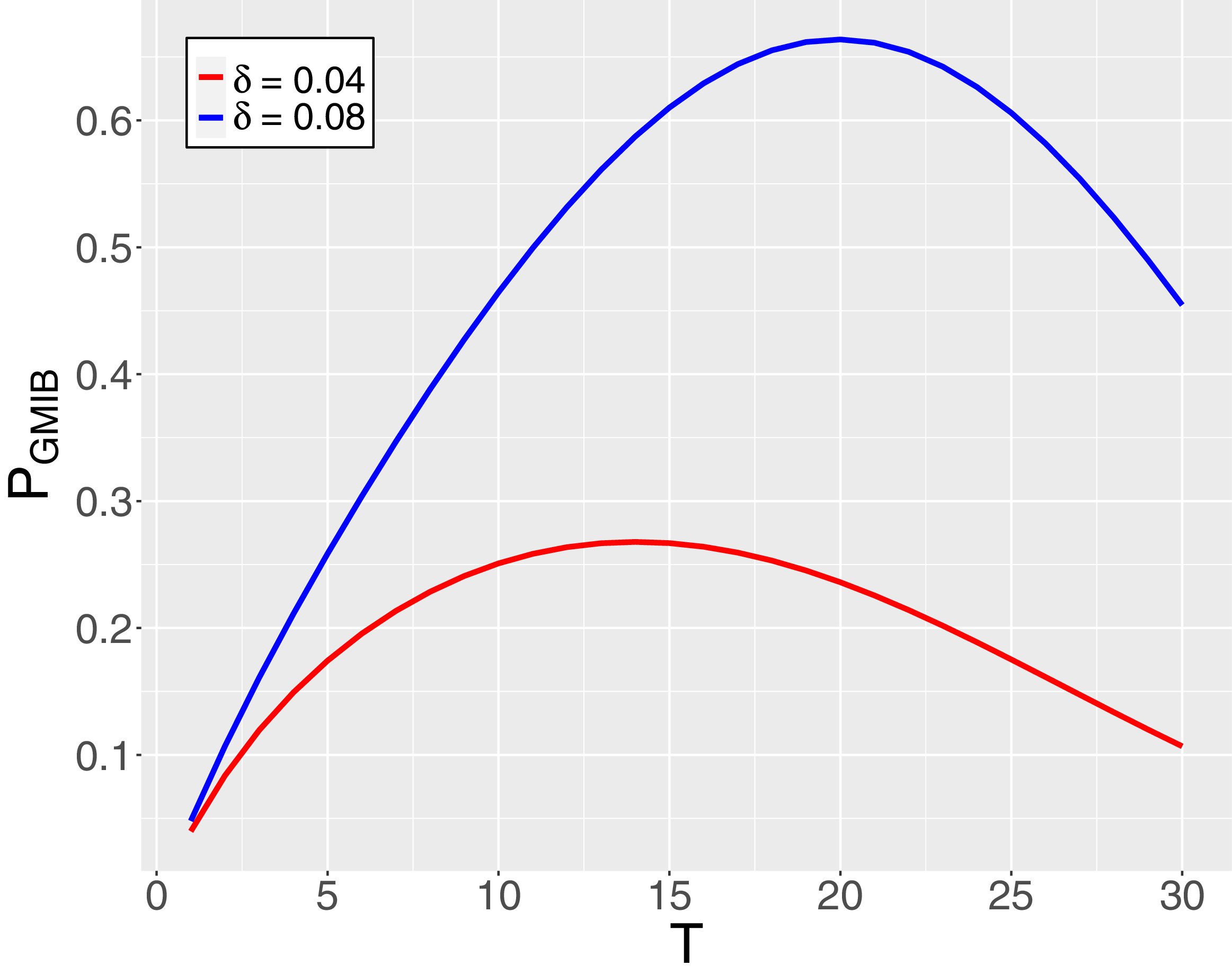

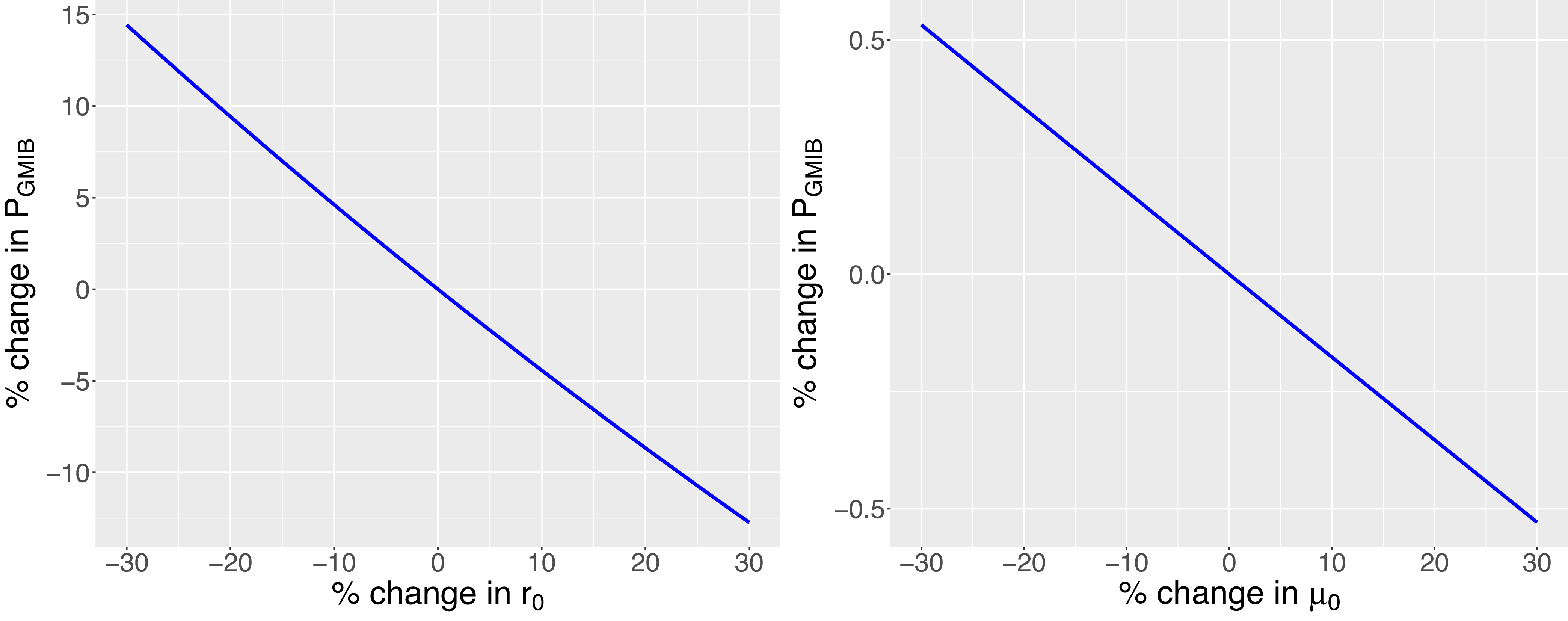


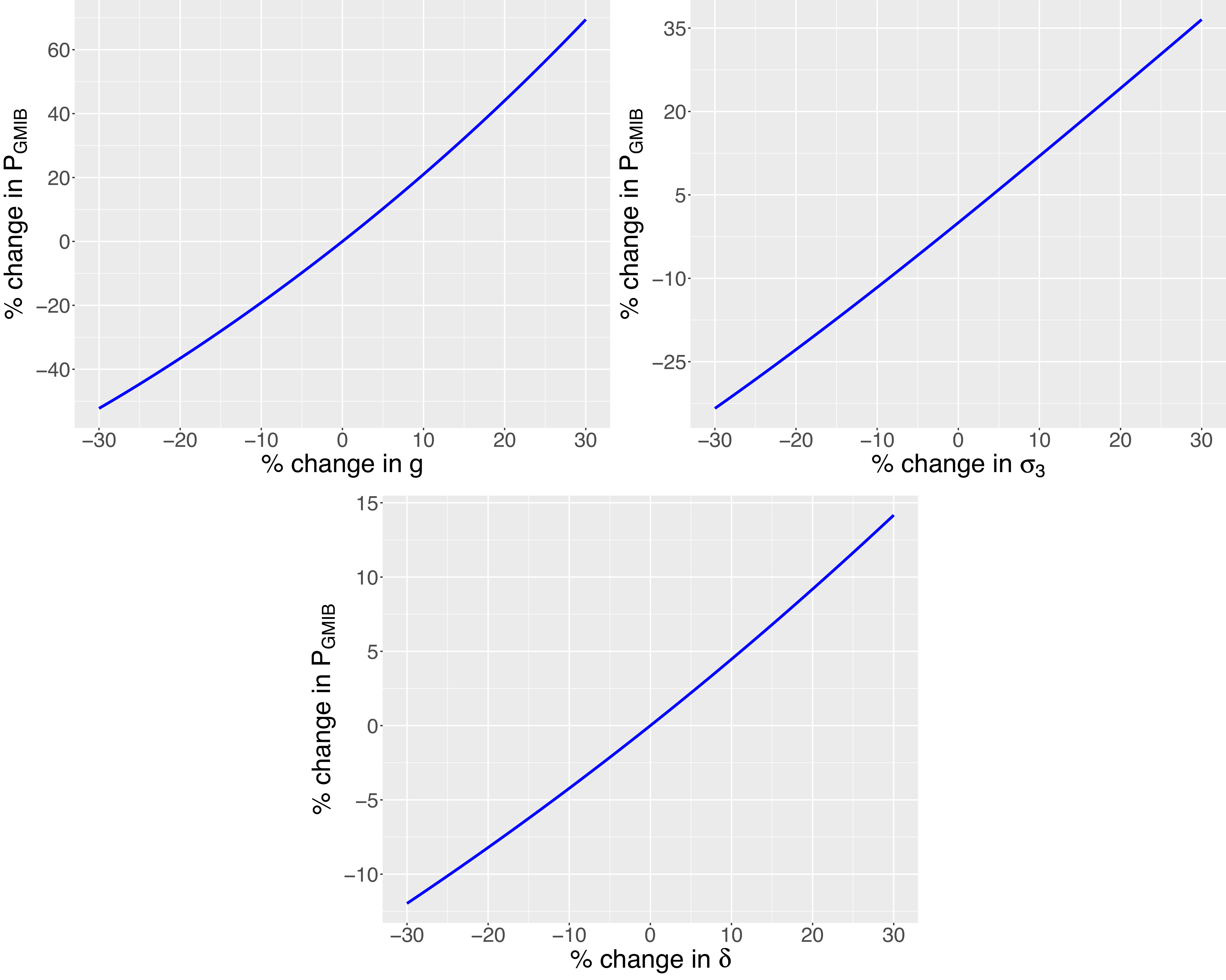


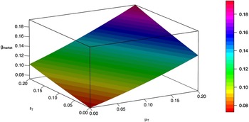


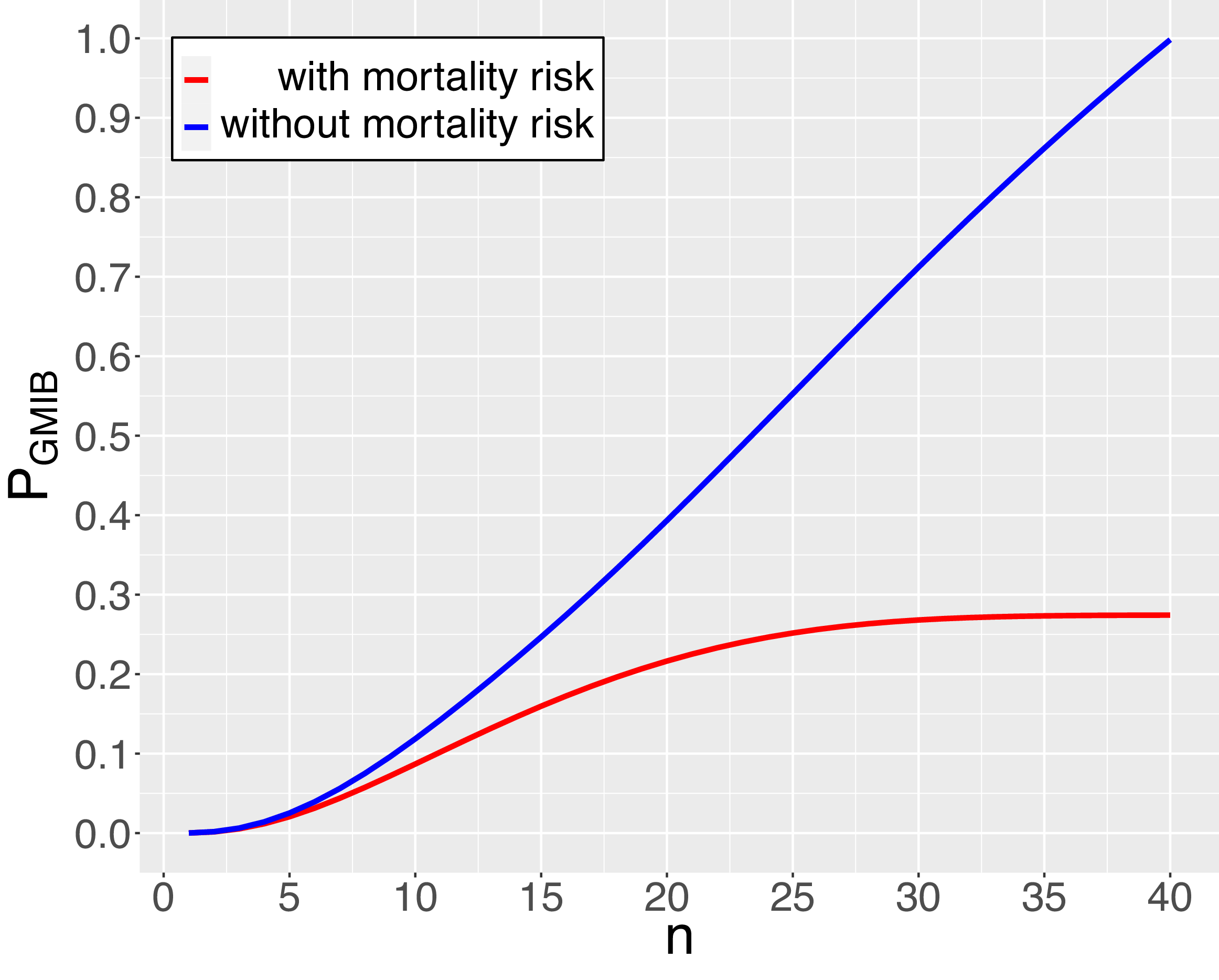
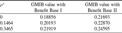




 Open access

