


1. Introduction
Since its adoption in New Zealand in 1991, the inflation targeting framework has permeated central banks around the world. The inflation targeting framework often features an announcement of the specific numerical target rate. Although the target rate of inflation has varied across time and countries, many central banks in advanced economies have recently converged to 2%.
However, the desirable value for the target rate of inflation is far from a settled issue. Within the academic literature, there is a wide range of estimates available, as pointed out by Diercks (Reference Diercks2019). Even focusing on the estimates emphasizing the role of the effective lower bound (ELB) constraint on the nominal interest rate—a key reason for preferring a small, but positive inflation rate often argued by central banks—the range of estimates remains wide. Even in the 2020s when the ELB constraint seems less of a concern than in the late 2000s and 2010s, some economists have argued for raising the inflation target from 2% that is dominant in advanced economies.Footnote 1
In this paper, we aim to contribute to the discussion of the optimal inflation target by examining the role of a previously neglected factor in the literature. The neglected factor is the possibility of expectations-driven liquidity traps (LTs). The previous literature has examined the implications of the ELB for the optimal inflation target, assuming that fundamental shocks drive the policy rate to the ELB. However, as shown by Benhabib et al. (Reference Benhabib, Schmitt-Grohe and Uribe2001) and Bullard (Reference Bullard2010) among many others, shifts in expectations (or sunspot shocks) can also drive the policy rate to the ELB.
Using a standard New Keynesian model, we show that the possibility of expectations-driven LTs reduces the optimal inflation target. This result can be understood as a relatively straightforward corollary to the well-known result in the literature on expectations-driven LTs about how a change in inflation expectations affects allocations in expectations-driven LTs. As shown by Mertens and Ravn (Reference Mertens and Ravn2014), Nakata and Schmidt (Reference Nakata and Schmidt2022), Bilbiie (Reference Bilbiie2022), Coyle et al. (Reference Coyle, Maezono, Nakata and Schmidt2023), higher inflation expectations—whether they are induced by a higher inflation target, forward guidance, or an increase in uncertainty—lower output and inflation in the expectations-driven LTs. Thus, the optimal inflation target is lower when the economy can fall into LTs due to shifts in expectations than otherwise.
Using a stylized, but calibrated model, we also show in the Online Appendix that even a very small probability of expectations-driven LTs nontrivially lowers the optimal inflation target. Under various calibrations of our baseline model with a two-state demand shock, a 0.1% (quarterly) probability of falling into expectations-driven LTs typically lowers the optimal inflation target by more than 1 percentage point. With a 0.5% probability of expectations-driven LTs, the optimal inflation target is typically slightly negative. In an alternative model with an AR(1) demand shock, 0.1% and 0.5% probabilities of falling into expectations-driven LTs lower the optimal inflation target by 0.6 percentage points and 0.8 percentage points, respectively.
Our analysis is motivated by the observation that Japan’s prolonged ELB experience may be primarily driven by self-fulfilling expectations rather than fundamental shocks (see, among others, Aruoba et al. (Reference Aruoba, Cuba-Borda and Schorfheide2018); Bullard (Reference Bullard2010)).Footnote 2 In Japan, both the output gap and inflation have been positive in the past few years. However, before that, inflation rates and the output gap had been negative for almost two decades. The combination of a slightly negative output gap and mild deflation with the nominal interest rate at the ELB constraint is consistent with the expectations-driven LT in the standard New Keynesian model. As we have learned over the past decade, what happens in Japan—though it may initially seem a theoretical curiosity for other countries—may happen in other countries years later. Thus, our analysis will be relevant for thinking about the optimal inflation target not only in Japan, but also in other countries.Footnote 3
Myriad factors that influence the optimal inflation target of an economy are absent in our model.Footnote 4 In this paper, our goal is not to come up with a sensible policy recommendation about whether to change the inflation target of 2% currently adopted by many central banks. Rather, our goal is to highlight a factor that has been neglected in the literature and examine its quantitative relevance.
Our paper is related to a set of papers that analyze the implications of alternative inflation targets in the interest rate feedback rule for the dynamics and welfare of economies with the ELB constraint. Earlier research on this topic includes Reifschneider and Williams (Reference Reifschneider and Williams2000) and Coenen et al. (Reference Coenen, Orphanides and Wieland2004) who use the FRB/US model—a large-scale macroeconometric model of the US economy—to analyze how the volatilities of output and inflation are affected by the level of the inflation target.Footnote
5
Our paper is most closely related to recent papers that compute the optimal inflation target in DSGE models, such as Andrade et al. (Reference Andrade, Galí, Bihan and Matheron2019); Blanco (Reference Blanco2021); Carreras et al. (Reference Carreras, Coibion, Gorodnichenko and Wieland2016); Coibion et al. (Reference Coibion, Gorodnichenko and Wieland2012); Hirata et al. (Reference Hirata, Mineyama and Nishizaki2022); and Mineyama (Reference Mineyama2022).Footnote
6 $^{,}$
Footnote
7
None of these papers allows for expectations-driven LTs. Our focus is the implications of expectations-driven LTs for the optimal inflation target.Footnote
8
$^{,}$
Footnote
7
None of these papers allows for expectations-driven LTs. Our focus is the implications of expectations-driven LTs for the optimal inflation target.Footnote
8
Our paper is related to papers analyzing expectations-driven LTs. Some papers are focused on analyzing what policies could eliminate this LT. Examples include Alstadheim and Henderson (Reference Alstadheim and Henderson2006), Armenter (Reference Armenter2017); Benhabib et al. (Reference Benhabib, Schmitt-Grohe and Uribe2002), Schmidt (Reference Schmidt2016); Schmitt-Grohe and Uribe (Reference Schmitt-Grohe and Uribe2013), Sugo and Ueda (Reference Sugo and Ueda2008), Nakata and Schmidt (Reference Nakata and Schmidt2022), and Tamanyu (Reference Tamanyu2022). Other papers are focused on the dynamics in and out of this LT. Examples include Aruoba et al. (Reference Aruoba, Cuba-Borda and Schorfheide2018), Bilbiie (Reference Bilbiie2022), Cuba-Borda and Singh (Reference Cuba-Borda and Singh2024), Hirose (Reference Hirose2007), Hirose (Reference Hirose2020), and Schmitt-Grohe and Uribe (Reference Schmitt-Grohe and Uribe2017). The novelty of our paper is that we examine the implications of expectations-driven LTs for the optimal inflation target.
The rest of the paper is organized as follows. Section 2 describes our baseline model and its calibration. Section 3 describes the results from our baseline model. Section 4 concludes.
2. Model
We use a nonlinear New Keynesian model with Rotemberg pricing. Because the model is standard, we relegate the details of the model to Online Appendix A. The equilibrium conditions of the model are given by
 \begin{equation} C_{t}^{-\chi _{c}} = \beta \delta _{t}R_{t}\mathrm{E_{t}}C_{t+1}^{-\chi _{c}}\Pi _{t+1}^{-1}, \end{equation}
 \begin{equation} w_{t}=N_{t}^{\chi _{n}}C_{t}^{\chi _{c}}, \end{equation}
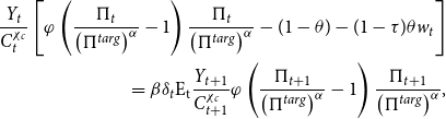 \begin{equation} \begin{aligned} \frac {Y_{t}}{C_{t}^{\chi _{c}}}\left [\varphi \left (\frac {\Pi _{t}}{\bigl (\Pi ^{targ}\bigr )^{\alpha }}-1\right )\frac {\Pi _{t}}{\bigl (\Pi ^{targ}\bigr )^{\alpha }} - (1-\theta )- (1-\tau )\theta w_{t}\right ]\\ \hspace {6em}= \beta \delta _{t}\mathrm{E_{t}}\frac {Y_{t+1}}{C_{t+1}^{\chi _{c}}}\varphi \left (\frac {\Pi _{t+1}}{\bigl (\Pi ^{targ}\bigr )^{\alpha }}-1\right )\frac {\Pi _{t+1}}{\bigl (\Pi ^{targ}\bigr )^{\alpha }}, \end{aligned} \end{equation}
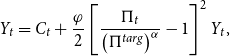 \begin{equation} Y_{t} = C_{t} + \frac {\varphi }{2}\left [\frac {\Pi _{t}}{\bigl (\Pi ^{targ}\bigr )^{\alpha }}-1\right ]^{2}Y_{t}, \end{equation}
 \begin{equation} Y_{t}=N_{t}, \end{equation}
 \begin{equation} R_{t} = \max \left [R_{ELB}, \quad \frac {\Pi ^{targ}}{\beta \delta _t}\left (\frac {\Pi _{t}}{\Pi ^{targ}}\right )^{\phi _{\pi }}\right ]. \end{equation} $C_{t}$
,
$C_{t}$
, $N_{t}$
,
$N_{t}$
, $Y_{t}$
,
$Y_{t}$
, $w_{t}$
,
$w_{t}$
, $\Pi _{t}$
, and
$\Pi _{t}$
, and $R_{t}$
are consumption, labor supply, output, real wage, inflation, and the policy rate, respectively. Equation (1) is the consumption Euler equation, equation (2) is the intratemporal optimality condition of the household, and equation (3) is the optimality condition of the intermediate good producing firms relating today’s inflation to real marginal cost today and expected inflation tomorrow (forward-looking Phillips curve). Equation (4) is the aggregate resource constraint capturing the resource cost of price adjustment, equation (5) is the aggregate production function, and equation (6) is the interest-rate feedback rule where
$R_{t}$
are consumption, labor supply, output, real wage, inflation, and the policy rate, respectively. Equation (1) is the consumption Euler equation, equation (2) is the intratemporal optimality condition of the household, and equation (3) is the optimality condition of the intermediate good producing firms relating today’s inflation to real marginal cost today and expected inflation tomorrow (forward-looking Phillips curve). Equation (4) is the aggregate resource constraint capturing the resource cost of price adjustment, equation (5) is the aggregate production function, and equation (6) is the interest-rate feedback rule where $\Pi ^{targ}$
is the central bank’s inflation target.
$\Pi ^{targ}$
is the central bank’s inflation target.
Note that the intercept of the interest-rate feedback rule is time-varying and depends on $\delta _{t}$
. Under this policy rule, the effect that the discount rate shock has on the economy through the consumption Euler equation is fully offset by a corresponding movement in the policy rate, as under optimal policy, unless the ELB constraint binds. This specification of the policy rule is often used in the ELB literature (see, for example, Boneva et al. (Reference Boneva, Braun and Waki2016); Eggertsson (Reference Eggertsson2011)).
$\delta _{t}$
. Under this policy rule, the effect that the discount rate shock has on the economy through the consumption Euler equation is fully offset by a corresponding movement in the policy rate, as under optimal policy, unless the ELB constraint binds. This specification of the policy rule is often used in the ELB literature (see, for example, Boneva et al. (Reference Boneva, Braun and Waki2016); Eggertsson (Reference Eggertsson2011)).
We allow for a form of indexation in the specification of the price adjustment cost. Specifically, the price adjustment cost is a quadratic function of $\Pi _{t}/(\Pi ^{targ})^{\alpha }$
. If the indexation parameter,
$\Pi _{t}/(\Pi ^{targ})^{\alpha }$
. If the indexation parameter, $\alpha$
, is 1, there is no steady state cost of a nonzero inflation target. The smaller the indexation parameter is, the larger the steady state cost of a nonzero inflation target becomes. Thus, holding all other parameter values fixed, an increase in
$\alpha$
, is 1, there is no steady state cost of a nonzero inflation target. The smaller the indexation parameter is, the larger the steady state cost of a nonzero inflation target becomes. Thus, holding all other parameter values fixed, an increase in $\alpha$
increases the optimal inflation target. The key mechanism of our model—a higher inflation target lowers consumption and inflation in the deflationary regime—does not depend on the value of
$\alpha$
increases the optimal inflation target. The key mechanism of our model—a higher inflation target lowers consumption and inflation in the deflationary regime—does not depend on the value of $\alpha$
, as shown in Online Appendix D. However, as we will discuss shortly in Section 2.1, one of our calibration principles is to make the optimal inflation target 2% in the model without expectations-driven LTs; thus, it is necessary to allow for some degree of price indexation to achieve that goal.Footnote
9
$\alpha$
, as shown in Online Appendix D. However, as we will discuss shortly in Section 2.1, one of our calibration principles is to make the optimal inflation target 2% in the model without expectations-driven LTs; thus, it is necessary to allow for some degree of price indexation to achieve that goal.Footnote
9 $\delta _{t}$
is an exogenous shock to the household’s discount rate and follows a two-state Markov process. It takes two values,
$\delta _{t}$
is an exogenous shock to the household’s discount rate and follows a two-state Markov process. It takes two values, $\delta _{N}=1$
and
$\delta _{N}=1$
and $\delta _{C}\gt 1$
, where
$\delta _{C}\gt 1$
, where $N$
and
$N$
and $C$
stand for normal and crisis states, respectively. The persistence of each state is given by
$C$
stand for normal and crisis states, respectively. The persistence of each state is given by
 \begin{align} & \text{Prob}(\delta _{t+1}=\delta _{N}|\delta _{t}=\delta _{N})= p_{N}, \end{align}
 \begin{align} & \text{Prob}(\delta _{t+1}=\delta _{C}|\delta _{t}=\delta _{C})= p_{C}. \end{align}
As pointed out by Benhabib et al. (Reference Benhabib, Schmitt-Grohe and Uribe2002) and as illustrated in Figure 1, the coexistence of the Euler equation—which implies a Fisher relation—and the truncated Taylor rule means that there are two steady states: one in which the policy rate is above zero and inflation is at the target (the target steady state), and one in which the policy rate is zero and the gross rate of inflation is $\beta$
(the deflationary steady state). With an exogenous crisis shock, we have one equilibrium associated with each steady state: one that fluctuates around the target steady state, and one that fluctuates around the deflationary steady state.
$\beta$
(the deflationary steady state). With an exogenous crisis shock, we have one equilibrium associated with each steady state: one that fluctuates around the target steady state, and one that fluctuates around the deflationary steady state.
Target and deflationary steady states.

Figure 4. Long description
Three line graphs depict the relationship between welfare and inflation target under different economic shock conditions. Panel A: Model with Crisis Shock Only. The line graph shows welfare on the vertical axis and inflation target on the horizontal axis. The welfare values range from -0.2 to 0, and the inflation target values range from -2 to 4. The graph shows a peak in welfare around an inflation target of 1. Panel B: Model with Sunspot Shock Only. The line graph shows welfare on the vertical axis and inflation target on the horizontal axis. The welfare values range from -2 to 0, and the inflation target values range from -2 to 4. The graph shows a steady decline in welfare as the inflation target increases. Panel C: Model with Crisis and Sunspot Shocks. The line graph shows welfare on the vertical axis and inflation target on the horizontal axis. The welfare values range from -2 to 0, and the inflation target values range from -2 to 4. The graph shows a decline in welfare as the inflation target increases, with a steeper decline compared to the other models.
As in Mertens and Ravn (Reference Mertens and Ravn2014) and Aruoba et al. (Reference Aruoba, Cuba-Borda and Schorfheide2018), we introduce a two-state Markov sunspot shock, $s_{t}$
, that allows the economy to transition between the target regime and the deflationary regime—the regime of an expectations-driven LT.
$s_{t}$
, that allows the economy to transition between the target regime and the deflationary regime—the regime of an expectations-driven LT. $s_{t}$
takes two values,
$s_{t}$
takes two values, $T$
and
$T$
and $D$
. When
$D$
. When $s_{t}=T$
, the economy is in the target regime. When
$s_{t}=T$
, the economy is in the target regime. When $s_{t}=D$
, the economy is in the deflationary regime. The persistence of each regime is given by
$s_{t}=D$
, the economy is in the deflationary regime. The persistence of each regime is given by
 \begin{align} & \text{Prob}(s_{t}=T|s_{t}=T)= p_{T}, \end{align}
 \begin{align} & \text{Prob}(s_{t}=D|s_{t}=D)= p_{D}. \end{align}
As discussed in Online Appendix B and analytically shown in Nakata and Schmidt (Reference Nakata and Schmidt2022), there are restrictions on these transition probabilities for the sunspot equilibrium to exist. In particular, the persistence parameters for both target and deflationary regimes must be sufficiently high for the sunspot equilibrium to exist. Throughout the paper, we restrict our attention to the set of parameter values consistent with the existence of the sunspot equilibrium.
The value function associated with an equilibrium is given by the expected discounted sum of future utility flows to the household. We can recursively write the value function as follows:
 \begin{equation} V_{t} = u(C_{t},N_{t}) + \beta \delta _{t}\mathrm{E_{t}}V_{t+1}, \end{equation}
where the per-period utility flow is given by
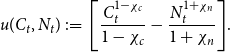 \begin{equation} u(C_{t},N_{t}) \;:\!=\; \Bigg [\frac {C_{t}^{1-\chi _{c}}}{1-\chi _{c}}-\frac {N_{t}^{1+\chi _{n}}}{1+\chi _{n}}\Bigg ]. \end{equation}
The welfare of the economy is measured by the unconditional expected value.
A recursive sunspot equilibrium of this stylized economy is given by a set of value and policy functions for $\{V(\delta ,s)$
,
$\{V(\delta ,s)$
, $C(\delta ,s)$
,
$C(\delta ,s)$
, $N(\delta ,s)$
,
$N(\delta ,s)$
, $Y(\delta ,s)$
,
$Y(\delta ,s)$
, $w(\delta ,s)$
,
$w(\delta ,s)$
, $\Pi (\delta ,s)$
,
$\Pi (\delta ,s)$
, $R(\delta ,s)\}$
such that (i) the equilibrium conditions described above are satisfied, (ii) the policy rate in the normal state of the target regime is above the ELB, and (iii) the policy rate in the normal state of the deflationary regime is at the ELB. That is, we require that
$R(\delta ,s)\}$
such that (i) the equilibrium conditions described above are satisfied, (ii) the policy rate in the normal state of the target regime is above the ELB, and (iii) the policy rate in the normal state of the deflationary regime is at the ELB. That is, we require that
 \begin{align} & R(\delta =\delta _{N},s=T) = \frac {\Pi ^{targ}}{\beta \delta _t}\left (\frac {\Pi (\delta =\delta _{N},s=T)}{\Pi ^{targ}}\right )^{\phi _{\pi }} \gt 1, \end{align}
 \begin{align} & R(\delta =\delta _{N},s=D) = 1, \end{align}
 \begin{align} & \frac {\Pi ^{targ}}{\beta \delta _t}\left (\frac {\Pi (\delta =\delta _{N},s=D)}{\Pi ^{targ}}\right )^{\phi _{\pi }} \lt 1. \end{align}
Following Mertens and Ravn (Reference Mertens and Ravn2014) and Aruoba et al. (Reference Aruoba, Cuba-Borda and Schorfheide2018), we focus on a recursive equilibrium in which the allocations today depend only on the realization of the crisis shock and the sunspot shock. In the deflationary regime, the Taylor principle is violated. As a result, there are infinitely many equilibria in the deflationary regime in which allocations today depend on past allocations and other sunspot shocks that are unrelated to the regime-switching sunspot shock that governs transitions between the target and deflationary regimes in this paper. Our equilibrium definition rules out these equilibria.Footnote 10
2.1 Calibration
Table 1 shows the baseline parameter values for the stylized model. We set $\chi _{c}$
,
$\chi _{c}$
, $\chi _{n}$
, and
$\chi _{n}$
, and $\theta$
to 1, 1, and 11, respectively. These are in line with the standard values in the literature. A production subsidy,
$\theta$
to 1, 1, and 11, respectively. These are in line with the standard values in the literature. A production subsidy, $\tau$
, is set to
$\tau$
, is set to $1/\theta$
so as to eliminate the distortion associated with monopolistic competition in the product market. With this value of
$1/\theta$
so as to eliminate the distortion associated with monopolistic competition in the product market. With this value of $\tau$
, the level of consumption and labor supply is efficient if the inflation target is 0% and if there are no shocks. For the policy rule, the inflation response coefficient,
$\tau$
, the level of consumption and labor supply is efficient if the inflation target is 0% and if there are no shocks. For the policy rule, the inflation response coefficient, $\phi _{\pi }$
, is set to 2 and the ELB,
$\phi _{\pi }$
, is set to 2 and the ELB, $R_{ELB}$
, is set to 1. While we solve our model under a number of different values of the inflation target parameter to determine the optimal inflation target, we will closely examine the dynamics of the model under 0% and 2% inflation targets to understand the key forces of the model.
$R_{ELB}$
, is set to 1. While we solve our model under a number of different values of the inflation target parameter to determine the optimal inflation target, we will closely examine the dynamics of the model under 0% and 2% inflation targets to understand the key forces of the model.
Conditional on the aforementioned parameters and the persistence parameters that will be discussed shortly, the price adjustment cost parameter ( $\varphi$
), the degree of indexation (
$\varphi$
), the degree of indexation ( $\alpha$
), and the size of the crisis shock (
$\alpha$
), and the size of the crisis shock ( $\delta _{C}$
) are chosen so that (i) consumption falls about 7% and inflation declines by about 2 percentage points in the crisis state of the target regime, and (ii) the optimal inflation target is 2% in the absence of the sunspot shock. The severity of a crisis is in line with those considered in Boneva et al. (Reference Boneva, Braun and Waki2016) and Hills and Nakata (Reference Hills and Nakata2018).
$\delta _{C}$
) are chosen so that (i) consumption falls about 7% and inflation declines by about 2 percentage points in the crisis state of the target regime, and (ii) the optimal inflation target is 2% in the absence of the sunspot shock. The severity of a crisis is in line with those considered in Boneva et al. (Reference Boneva, Braun and Waki2016) and Hills and Nakata (Reference Hills and Nakata2018).
Our calibration for $\varphi$
and
$\varphi$
and $\alpha$
implies that the share of price adjustment costs in terms of output is 1.0% in the standard steady state when the target rate of inflation is 2%. Although it is difficult to directly measure the resource cost of price adjustment, this value is close to the value from the empirical evidence by Levy et al. (Reference Levy, Bergen, Dutta and Venable1997) on menu costs in the USA in 1991–92 when inflation averaged 2.6%—which is 0.7%. The share is 0.26 % in our model at the deflationary steady state where inflation is minus 1%. This value is close to the value reported in Boneva et al. (Reference Boneva, Braun and Waki2016)—which is 0.15%.
$\alpha$
implies that the share of price adjustment costs in terms of output is 1.0% in the standard steady state when the target rate of inflation is 2%. Although it is difficult to directly measure the resource cost of price adjustment, this value is close to the value from the empirical evidence by Levy et al. (Reference Levy, Bergen, Dutta and Venable1997) on menu costs in the USA in 1991–92 when inflation averaged 2.6%—which is 0.7%. The share is 0.26 % in our model at the deflationary steady state where inflation is minus 1%. This value is close to the value reported in Boneva et al. (Reference Boneva, Braun and Waki2016)—which is 0.15%.
The persistence of the normal state and the persistence of the crisis state are set to 0.995 and 0.75, respectively. The normal state persistence of 0.995 implies that the crisis shock hits the economy, on average, once in 50 years. The crisis state persistence of 0.75 implies that the crisis shock lasts for one year on average. We will also consider other values of $p_{C}$
and
$p_{C}$
and $p_{N}$
for sensitivity analyses.
$p_{N}$
for sensitivity analyses.
Baseline parameter values for the stylized model

As a baseline, we set the persistence of the deflationary regime to 0.975, which implies an expected duration of the deflationary regime of 10 years. With this persistence, the decline of output in the normal state of the deflationary regime is about 1%.Footnote 11 We will also consider some alternative values for the deflationary regime persistence for a sensitivity analysis. We use the target regime persistence of 0.995—which implies an expected duration of the target regime of 50 years—as our baseline, but we compute the optimal inflation target for a wide range of values to understand how the probability of moving from the target regime to the deflationary regime affects the optimal inflation target.
In the model, there are four states (two states for the sunspot shock and two states for the natural rate shock); thus, solving for the policy functions amounts to solving a system of nonlinear equations. We use MATLAB’s built-in nonlinear equation solver, fsolve, to solve our model.
3. Results
We first discuss how the inflation target affects allocations and welfare in a version of the model with a crisis shock only. Next, we discuss how the inflation target affects allocations and welfare in a version of the model with a sunspot shock only. Finally, we discuss the optimal inflation target in the model with both a crisis shock and a sunspot shock.
3.1 Optimal inflation target in the model with a crisis shock only
Figure 2 shows the dynamics of the economy in the model with a crisis shock only under 0% and 2% inflation targets. The economy is in the normal state from period 1 to period 5. The crisis shock hits the economy in period 6 and persists until period 10. The economy is back in the normal state thereafter.
When the inflation target is zero—the case shown by the solid black lines—inflation and the output gap are close to the target and the policy rate is positive in the normal state.Footnote 12 When the crisis shock hits the economy, the central bank lowers the policy rate, trying to offset the adverse effects of the shock, but the ELB constraint prevents the central bank from fully neutralizing the effects of the shock: Inflation and consumption decline and the policy rate is at the ELB.
Allocations under a crisis shock.

Figure 4. Long description
Three line graphs depict the relationship between welfare and inflation target under different economic shock conditions. Panel A: Model with Crisis Shock Only. The line graph shows welfare on the vertical axis and inflation target on the horizontal axis. The welfare values range from -0.2 to 0, and the inflation target values range from -2 to 4. The graph shows a peak in welfare around an inflation target of 1. Panel B: Model with Sunspot Shock Only. The line graph shows welfare on the vertical axis and inflation target on the horizontal axis. The welfare values range from -2 to 0, and the inflation target values range from -2 to 4. The graph shows a steady decline in welfare as the inflation target increases. Panel C: Model with Crisis and Sunspot Shocks. The line graph shows welfare on the vertical axis and inflation target on the horizontal axis. The welfare values range from -2 to 0, and the inflation target values range from -2 to 4. The graph shows a decline in welfare as the inflation target increases, with a steeper decline compared to the other models.
AD and AS curves in the crisis state and in the deflationary regime.

Figure 4. Long description
Three line graphs depict the relationship between welfare and inflation target under different economic shock conditions. Panel A: Model with Crisis Shock Only. The line graph shows welfare on the vertical axis and inflation target on the horizontal axis. The welfare values range from -0.2 to 0, and the inflation target values range from -2 to 4. The graph shows a peak in welfare around an inflation target of 1. Panel B: Model with Sunspot Shock Only. The line graph shows welfare on the vertical axis and inflation target on the horizontal axis. The welfare values range from -2 to 0, and the inflation target values range from -2 to 4. The graph shows a steady decline in welfare as the inflation target increases. Panel C: Model with Crisis and Sunspot Shocks. The line graph shows welfare on the vertical axis and inflation target on the horizontal axis. The welfare values range from -2 to 0, and the inflation target values range from -2 to 4. The graph shows a decline in welfare as the inflation target increases, with a steeper decline compared to the other models.
The dashed blue lines in Figure 2 show the dynamics of the economy when the inflation target is 2%. In the normal state, a higher inflation target implies higher inflation and a higher policy rate because the Taylor rule is operative. Higher inflation increases the price adjustment cost and thus lowers consumption, though these effects are very small in our baseline calibration.Footnote 13 Higher normal state inflation leads to a lower expected real interest rate in the crisis state in which the policy rate is constrained at the ELB, mitigating the declines in inflation and consumption in the crisis state: In the crisis state, inflation and consumption are higher under the 2% inflation target than under the 0% inflation target.
These favorable effects of a higher inflation target on crisis state inflation and consumption can be fully understood by examining how an increase in the inflation target affects crisis state AD and AS curves—the set of consumption–inflation pairs consistent with the consumption Euler equation and the Phillips curve in the crisis state, respectively. The left panel of Figure 3 shows AD and AS curves in the crisis state. A higher inflation target means that inflation is higher in the normal state, because the Taylor rule operates in the normal state. When there is a positive probability of returning to the normal state—holding the crisis state inflation rate fixed—higher normal state inflation leads to higher inflation expectations and thus a lower expected real rate in the crisis state in which the ELB binds. The consumption Euler equation requires that crisis state consumption increases when the expected real rate declines. Thus, the AD curve shifts to the right. At the same time, the Phillips curve requires that crisis state inflation increases with normal state inflation—holding crisis state consumption fixed—because firms are forward-looking in their pricing decision. Thus, the AS curve shifts up. Taken together, these shifts in the AD and AS curves mean that, in equilibrium, an increase in the inflation target leads to higher inflation and consumption in the crisis state.
All told, there is a simple trade-off in adjusting the inflation target in this model with a crisis shock only. On the one hand, a higher inflation target is associated with inefficiently low consumption in the normal state. On the other hand, a higher inflation target is associated with better stabilization outcomes in the crisis state.Footnote 14 Reflecting this trade-off, welfare is a concave function of the inflation target, as shown in the left panel of Figure 4. As discussed earlier, the degree of indexation is chosen so that welfare attains its maximum at 2%, indicated by the vertical blue line.
3.2 Optimal inflation target in the model with a sunspot shock only
Figure 5 shows the dynamics of the model with a sunspot shock only. The economy is in the target regime from period 1 to period 5. The sunspot shock hits the economy at period 6 and stays there until period 10—that is, the economy is in the deflationary regime from period 6 to 10. The economy is back in the target regime thereafter.
Welfare and the inflation target. Note: For each model, welfare is measured by the perpetual consumption transfer—expressed as a percentage of consumption at the deterministic steady state of the target regime—we need to give to the household in the version of the economy without the ELB so that it is as well-off as the household in the economy with the ELB.

Figure 4. Long description
Three line graphs depict the relationship between welfare and inflation target under different economic shock conditions. Panel A: Model with Crisis Shock Only. The line graph shows welfare on the vertical axis and inflation target on the horizontal axis. The welfare values range from -0.2 to 0, and the inflation target values range from -2 to 4. The graph shows a peak in welfare around an inflation target of 1. Panel B: Model with Sunspot Shock Only. The line graph shows welfare on the vertical axis and inflation target on the horizontal axis. The welfare values range from -2 to 0, and the inflation target values range from -2 to 4. The graph shows a steady decline in welfare as the inflation target increases. Panel C: Model with Crisis and Sunspot Shocks. The line graph shows welfare on the vertical axis and inflation target on the horizontal axis. The welfare values range from -2 to 0, and the inflation target values range from -2 to 4. The graph shows a decline in welfare as the inflation target increases, with a steeper decline compared to the other models.
Allocations under a sunspot shock.

Figure 4. Long description
Three line graphs depict the relationship between welfare and inflation target under different economic shock conditions. Panel A: Model with Crisis Shock Only. The line graph shows welfare on the vertical axis and inflation target on the horizontal axis. The welfare values range from -0.2 to 0, and the inflation target values range from -2 to 4. The graph shows a peak in welfare around an inflation target of 1. Panel B: Model with Sunspot Shock Only. The line graph shows welfare on the vertical axis and inflation target on the horizontal axis. The welfare values range from -2 to 0, and the inflation target values range from -2 to 4. The graph shows a steady decline in welfare as the inflation target increases. Panel C: Model with Crisis and Sunspot Shocks. The line graph shows welfare on the vertical axis and inflation target on the horizontal axis. The welfare values range from -2 to 0, and the inflation target values range from -2 to 4. The graph shows a decline in welfare as the inflation target increases, with a steeper decline compared to the other models.
When the inflation target is zero—shown by the solid black lines—the policy rate is positive, inflation is essentially zero, and consumption is slightly above the efficient level in the target regime. When the economy moves to the deflationary regime, the policy rate hits the ELB, inflation falls by 1 percentage point, and consumption declines by half a percentage point.
When the inflation target is 2%—shown by the dashed blue lines—the policy rate is close to 3%, inflation is slightly below 2%, and consumption is slightly above the efficient level in the target regime. When the economy moves to the deflationary regime, the policy rate hits the ELB and inflation and consumption fall. Inflation is about negative 1.5% and consumption is about 3% below the efficient level under the 2% inflation target. Inflation and consumption are nontrivially lower in the deflationary regime under the 2% inflation target than under the 0% inflation target.
A higher inflation target lowers inflation and consumption in the deflationary regime through the following mechanism. A higher inflation target means that inflation is higher in the target regime, because the Taylor rule operates in the target regime. When there is a positive probability of moving to the target regime—holding the deflationary-regime inflation rate fixed—higher target-regime inflation leads to higher inflation expectations in the deflationary regime. The Phillips curve then requires that an increase in expected inflation leads to a decline in the marginal cost of production—which depends on consumption and output—holding the deflationary-regime inflation rate fixed. For the marginal cost to decline, the real interest rate has to increase. When the policy rate is constrained at the ELB, the real interest rate increases only if expected inflation declines. For expected inflation to decline, actual inflation needs to decline. In equilibrium, both actual and expected inflation have to decline in the deflationary regime when the inflation target increases.
The adverse effects of a higher inflation target on the deflationary-regime inflation and consumption can also be understood through AS and AD curves in the deflationary regime, which are shown in the right panel of Figure 3. As in the model with a crisis shock only, a higher inflation target means higher inflation in the target regime. When there is a positive probability of returning to the target regime—holding the deflationary-regime inflation rate fixed—higher target regime inflation means higher inflation expectations, a lower expected real rate, and higher consumption in the deflationary regime.Footnote 15 Thus, the AD curve shifts to the right. Similar to what we saw in the model with a crisis shock only, the Phillips curve requires that higher target regime inflation leads to higher deflationary regime inflation, holding the deflationary regime consumption fixed, causing the AS curve to shift up. These shifts in the AD and AS curves mean that, in equilibrium, a higher inflation target leads to lower inflation and consumption in the deflationary regime.
Although the effects of a higher inflation target on the AD and AS curves in the deflationary regime are the same as those in the crisis state we examined earlier, they have the opposite equilibrium implications in the deflationary regime. The opposite implications emerge because the AD curve is steeper than the AS curve in the crisis state, whereas the AD curve is flatter than the AS curve in the deflationary regime.
All told, in the model with a sunspot shock only, a higher inflation target worsens the allocations in both the target and deflationary regimes. Thus, welfare is higher when the inflation target is lower, as shown in the middle panel of Figure 4.Footnote 16
3.3 Model with both a crisis shock and a sunspot shock
Because a higher inflation target is associated with lower welfare in the model with a sunspot shock, if we introduce the sunspot shock to the model with a crisis shock only, the optimal inflation target declines. The solid line in the right panel of Figure 4 shows how the welfare of the economy depends on the inflation target in the model with both a crisis shock and a sunspot shock. The welfare is maximized at negative $0.6$
%, the lowest value of the inflation target consistent with the existence of the sunspot equilibrium and
$0.6$
%, the lowest value of the inflation target consistent with the existence of the sunspot equilibrium and $2.6$
percentage points lower than that in the economy with a crisis shock only and essentially the same as that in the economy with a sunspot shock only.
$2.6$
percentage points lower than that in the economy with a crisis shock only and essentially the same as that in the economy with a sunspot shock only.
Optimal inflation target with alternative probabilities of moving to the deflationary regime.

Figure 4. Long description
Three line graphs depict the relationship between welfare and inflation target under different economic shock conditions. Panel A: Model with Crisis Shock Only. The line graph shows welfare on the vertical axis and inflation target on the horizontal axis. The welfare values range from -0.2 to 0, and the inflation target values range from -2 to 4. The graph shows a peak in welfare around an inflation target of 1. Panel B: Model with Sunspot Shock Only. The line graph shows welfare on the vertical axis and inflation target on the horizontal axis. The welfare values range from -2 to 0, and the inflation target values range from -2 to 4. The graph shows a steady decline in welfare as the inflation target increases. Panel C: Model with Crisis and Sunspot Shocks. The line graph shows welfare on the vertical axis and inflation target on the horizontal axis. The welfare values range from -2 to 0, and the inflation target values range from -2 to 4. The graph shows a decline in welfare as the inflation target increases, with a steeper decline compared to the other models.
The extent to which the sunspot shock lowers the inflation target depends on how likely it is for the economy to be in the deflationary regime. In Figure 6, we show how the optimal inflation target varies with the probability of moving from the target regime to the deflationary regime under our baseline calibration ( $1-p_T$
). According to the figure, the optimal inflation target declines as the probability of moving from the target regime to the deflationary regime increases for any given persistence of the deflationary regime. When the transition probability is 0.1% and 0.2%, the optimal inflation target is
$1-p_T$
). According to the figure, the optimal inflation target declines as the probability of moving from the target regime to the deflationary regime increases for any given persistence of the deflationary regime. When the transition probability is 0.1% and 0.2%, the optimal inflation target is $0.1$
% and negative
$0.1$
% and negative $0.3$
%, respectively.
$0.3$
%, respectively.
The effect of the sunspot shock on the optimal inflation target dominates that of the crisis shock because the unconditional probability of being in the deflationary regime is much higher than the unconditional probability of being in the crisis state, unless the transition probability to the deflationary regime ( $1-p_{T}$
) is very small. To see this point, Figure 7 shows the unconditional probabilities of being in the deflationary regime for a range of
$1-p_{T}$
) is very small. To see this point, Figure 7 shows the unconditional probabilities of being in the deflationary regime for a range of $1-p_{T}$
(solid black line) with other transition probability parameters fixed at their baseline values. Under our baseline value,
$1-p_{T}$
(solid black line) with other transition probability parameters fixed at their baseline values. Under our baseline value, $1-p_{T}=0.005$
, the unconditional probability of the deflationary regime is 16.6%, about 8 times as large as the unconditional probability of the crisis state, which is 2% as shown by the dashed black line. Only when
$1-p_{T}=0.005$
, the unconditional probability of the deflationary regime is 16.6%, about 8 times as large as the unconditional probability of the crisis state, which is 2% as shown by the dashed black line. Only when $1-p_{T}$
is very close to 0 (smaller than 0.0005 to be specific) is the unconditional probability of the crisis state higher than the unconditional probability of the deflationary regime.
$1-p_{T}$
is very close to 0 (smaller than 0.0005 to be specific) is the unconditional probability of the crisis state higher than the unconditional probability of the deflationary regime.
Unconditional probability of being in a crisis state or deflationary regime.

Figure 4. Long description
Three line graphs depict the relationship between welfare and inflation target under different economic shock conditions. Panel A: Model with Crisis Shock Only. The line graph shows welfare on the vertical axis and inflation target on the horizontal axis. The welfare values range from -0.2 to 0, and the inflation target values range from -2 to 4. The graph shows a peak in welfare around an inflation target of 1. Panel B: Model with Sunspot Shock Only. The line graph shows welfare on the vertical axis and inflation target on the horizontal axis. The welfare values range from -2 to 0, and the inflation target values range from -2 to 4. The graph shows a steady decline in welfare as the inflation target increases. Panel C: Model with Crisis and Sunspot Shocks. The line graph shows welfare on the vertical axis and inflation target on the horizontal axis. The welfare values range from -2 to 0, and the inflation target values range from -2 to 4. The graph shows a decline in welfare as the inflation target increases, with a steeper decline compared to the other models.
The unconditional probability of the deflationary regime being much higher than the unconditional probability of the crisis state is a necessary by-product of the equilibrium existence conditions on the transition probabilities of the crisis shock and the sunspot shock. For an equilibrium to exist in the model with a crisis shock, the persistence of the crisis state has to be sufficiently low (Nakata (Reference Nakata2019); Online Appendix B); for an equilibrium to exist in the model with a sunspot shock, the persistence of the deflationary regime has to be sufficiently high (Nakata and Schmidt (Reference Nakata and Schmidt2022); Online Appendix B). Thus, unless the persistence of the target regime is very high—that is, it is very unlikely for an economy to fall into expectations-driven LTs—or the persistence of the normal state is very low—that is, it is very likely for an economy to be hit by a crisis shock—the unconditional probability of the deflationary regime is higher than the unconditional probability of the crisis state.
3.4 Sensitivity analysis
We have just seen that the extent to which the possibility of falling into an expectations-driven LT lowers the optimal inflation target depends on the likelihood of being in an expectations-driven LT relative to the likelihood of being in a fundamental-driven LT. Thus, the optimal inflation target is higher under alternative calibrations in which the unconditional probability of being in an expectations-driven LT is lower than that in our baseline calibration or those in which the unconditional probability of being in a fundamental-driven LT is higher than that in our baseline.
In the top-right, top-left, and bottom-left panels of Figure 8, we show two alternative calibrations of the model with lower deflationary regime persistence ( $p_{D}$
), lower crisis shock persistence (
$p_{D}$
), lower crisis shock persistence ( $p_{C}$
), and lower crisis shock frequency—equivalently, higher normal state persistence (
$p_{C}$
), and lower crisis shock frequency—equivalently, higher normal state persistence ( $p_{N}$
)—respectively. In each panel, these alternative calibrations are displayed by the dashed and dash-dotted lines. In the top-right and bottom-left panels, when we vary the crisis shock persistence and frequency, the crisis shock size, price adjustment cost (
$p_{N}$
)—respectively. In each panel, these alternative calibrations are displayed by the dashed and dash-dotted lines. In the top-right and bottom-left panels, when we vary the crisis shock persistence and frequency, the crisis shock size, price adjustment cost ( $\varphi$
), and the degree of indexation (
$\varphi$
), and the degree of indexation ( $\alpha$
) are adjusted to be consistent with the calibration principle outlined earlier.
$\alpha$
) are adjusted to be consistent with the calibration principle outlined earlier.
The top-left panel shows that the lower deflationary regime persistence is, the higher the optimal inflation target is. The top-right and bottom-left panels show that the higher the crisis persistence or the crisis frequency—both of which imply a higher unconditional probability of being in the crisis state—the higher the optimal inflation target.
Finally, in the bottom-right panel of Figure 8, we show two alternative calibrations—shown by the dashed and dash-dotted lines—in which the crisis shock size, $\varphi$
, and
$\varphi$
, and $\alpha$
are chosen so that the optimal inflation target is 0.5% and 1% in the model with the crisis shock only, respectively. This exercise is motivated by the possibility that the ELB is the only reason why the central bank aims for a positive inflation target and that the ELB accounts for only a part of the stated inflation target by central banks.Footnote
17
In these alternative calibrations, because the optimal inflation target is lower to begin with, the possibility of falling into the expectations-driven LT reduces the optimal inflation target by less than it does in the baseline calibration.
$\alpha$
are chosen so that the optimal inflation target is 0.5% and 1% in the model with the crisis shock only, respectively. This exercise is motivated by the possibility that the ELB is the only reason why the central bank aims for a positive inflation target and that the ELB accounts for only a part of the stated inflation target by central banks.Footnote
17
In these alternative calibrations, because the optimal inflation target is lower to begin with, the possibility of falling into the expectations-driven LT reduces the optimal inflation target by less than it does in the baseline calibration.
Optimal inflation target with alternative probabilities of moving to the deflationary regime.

Figure 4. Long description
Three line graphs depict the relationship between welfare and inflation target under different economic shock conditions. Panel A: Model with Crisis Shock Only. The line graph shows welfare on the vertical axis and inflation target on the horizontal axis. The welfare values range from -0.2 to 0, and the inflation target values range from -2 to 4. The graph shows a peak in welfare around an inflation target of 1. Panel B: Model with Sunspot Shock Only. The line graph shows welfare on the vertical axis and inflation target on the horizontal axis. The welfare values range from -2 to 0, and the inflation target values range from -2 to 4. The graph shows a steady decline in welfare as the inflation target increases. Panel C: Model with Crisis and Sunspot Shocks. The line graph shows welfare on the vertical axis and inflation target on the horizontal axis. The welfare values range from -2 to 0, and the inflation target values range from -2 to 4. The graph shows a decline in welfare as the inflation target increases, with a steeper decline compared to the other models.
4. Conclusion
In this paper, we examine how the possibility of falling into expectations-driven LTs affects the optimal inflation target. Using a calibrated New Keynesian model, we find that even a very small probability of expectations-driven LTs nontrivially lowers the optimal inflation target under a wide range of parameter values. Our paper highlights a factor that has been neglected in the literature and the policy debate regarding the optimal inflation target. Because myriad factors influence the judgment on whether central banks should increase their inflation target in light of the ELB consideration, caution is of course warranted in drawing any policy implications from our exercise.
One limitation of our analysis—shared by other papers on this topic—is that we are silent about why an economy may fall into the expectations-driven LT or why it may escape from it. In particular, we assume that the transition probabilities governing the sunspot shock are exogenous to the conduct of monetary policy. According to a common narrative of the Japanese economy by seasoned observers (see, for example, Hayakawa (Reference Hayakawa2016)), one rationale for the aggressive monetary policy easing in Japan that started in 2013—including an official adoption of the 2% inflation target—is that the aggressive easing may help push the Japanese economy out of the expectations-driven LT. While it is plausible that a change in some aspects of the monetary policy can affect the likelihood of falling into an expectations-driven LT, we followed the literature and excluded such a possibility in this paper. We leave the investigation of such a possibility to future research.
Supplementary material
The supplementary material for this article can be found at http://doi.org/10.1017/S1365100526101175.
Acknowledgements
We thank Roberto Billi, Pablo Cuba-Borda, Yasuo Hirose, Antoine Lepetit, Matthias Paustian, Sebastian Schmidt, and Yoichiro Tamanyu for useful discussions and suggestions. We also thank David Jenkins for his editorial assistance. We used large language models to correct grammatical errors and improve the readability of the manuscript.
Competing interests
The authors declare none.


 Open access

