


Introduction
The Southern Great Plains (SGP) includes portions of Texas, Oklahoma, and New Mexico (Kumar et al., Reference Kumar, Obour, Jha, Liu, Manuchehri, Holman and Stahlman2020) (Appendix Figure A1). SGP producers contend with hot summers, cold and dry winters, and uncertain rainfall (Hansen et al., Reference Hansen, Allen, Baumhardt and Lyon2012; Poland et al., Reference Poland, Patel-Weynand, Finch, Miniat, Hayes and Lopez2021). Approximately 80 percent of the SGP’s crop production is rainfed, with more than half of the currently irrigated farmland expected to transition to dryland production over the next few decades (USGS, 2016). The region’s agricultural land cover is primarily winter wheat, pasture, native prairie grasses, and switchgrass (Raz-Yaseef et al., Reference Raz-Yaseef, Billesbach, Fischer, Biraud, Gunter, Bradford and Torn2015). Corn and cotton are also grown in the area; however, corn typically requires irrigation, and cotton is not as frequently grown in a rotation with wheat relative to sorghum and soybean (Kumar et al., Reference Kumar, Liu, Boyer and Stahlman2019). Standard rainfed wheat cropping systems include winter wheat (Triticum aestivum L.) and summer fallow and winter wheat-summer crop-fallow systems. Summer crops used in rotation with wheat include soybean (Glycine max L. Merr.) and grain sorghum (Sorghum bicolor L.).
Weed pressure negatively affects revenue by reducing yield and increasing weed control costs. On average, over $11 billion (USD) a year is spent controlling weeds in agriculture (Hartfield et al., Reference Hartfield, Antle, Garrett, Izaurralde, Mader, Marshall, Nearing, Robertson and Ziska2014). Best weed management practices include scouting, cleaning equipment after harvest, and changing herbicide chemical mixes (Zhou et al., Reference Zhou, Roberts, Larson, Lambert, English, Mishra, Falconer, Hogan, Johnson and Reeves2016). Other weed management practices include manual removal, mechanical tillage, and cover crops, which may increase operating costs (Garrison et al., Reference Garrison, Miller, Ryan, Roxburgh and Shea2017; Livingston et al., Reference Livingston, Fenandez-Cornejo, Unger, Osteen, Schimmelpfennig, Park and Lambert2015). Among the practices mentioned, controlling weeds with herbicides is comparatively cost-effective and has relatively lower labor requirements (Clay, Reference Clay2021; Green, Reference Green2011; Jha et al., Reference Jha, Kumar, Godara and Chauhan2017; Shaw et al., Reference Shaw, Givens, Farno, Gerard, Jordan, Johnson, Weller, Young, Wilson and Owen2009).
No-till (NT) rainfed systems are familiar to some parts of the SGP. NT adoption on wheat acres has expanded in the SGP, increasing from 20 to 45 percent of planted wheat acres between 2000 and 2017 (Claassen et al., Reference Claassen, Bowman, McFadden, Smith and Wallander2018). NT soybean acres have increased from 35 to 40 percent of planted acres during the same period (Claassen et al., Reference Claassen, Bowman, McFadden, Smith and Wallander2018). NT and minimum tillage systems require more intensive and frequent herbicide use than conventional ones (Friedrich, Reference Friedrich2005). Double-crop systems may also have higher herbicide requirements (Kapusta, Reference Kapusta1979). Tilling is a short-term solution for controlling weeds. However, over the long term, there may be little difference in the effectiveness of conventional till or NT systems for managing weed populations (Friedrich, Reference Friedrich2005). For continuously seeded wheat, reduced tillage can increase weed control costs (Epplin et al., Reference Epplin, Al-Saakaf and Peeper1994; Bł&adot;zewicz-Wozniak et al., Reference Bł&adot;zewicz-Wozniak, Patkowska, Konopinski and Wach2016).
Wheat producers in the SGP contend with weed species such as kochia (Kochia scoparia (L.) A.J. Scott), Italian ryegrass [Lolium multiflorum ssp. Multiforum (Lam) Husnot], and horseweed (Conyza canadensis L.) (Heap, Reference Heap2020). Horseweed was not previously considered problematic in the SGP because it could be managed with tilling. Recently, horseweed has become a nuisance weed in this region due to the increased use of reduced tillage and NT (Crose et al., Reference Crose, Manuchehri and Baughman2020). SGP soybean and sorghum growers struggle with herbicide-resistant waterhemp [Amaranthus tuberculatus (Moq.) J.D. Sauer] and Palmer amaranth (Amaranthus palmeri S. Watson). Palmer amaranth is among the most problematic annual broadleaf species in the United States (US), affecting soybean, sorghum, corn, cotton, sunflower, wheat, and fallow acres (Kumar et al., Reference Kumar, Liu, Boyer and Stahlman2019). Palmer amaranth is particularly difficult to manage due to its fecundity, rapid growth, and adaptability. Once established, Palmer amaranth can decrease soybean yield between 19 and 80 percent and sorghum yield between 13 and 50 percent, depending on weed density (Korres et al., Reference Korres, Norsworthy, Mauromoustakos and Williams2020; Ward and Webster, Reference Ward and Webster2013).
This research compares the economic performance of rainfed wheat-fallow (WF) and wheat-double crop systems under varying intensities of competition with horseweed and Palmer amaranth. Economic performance is measured as per hectare net returns to WF and wheat-double crop systems under conventional till or NT cultivation. Net returns are compared over medium- (five years) and long-term (>5 years) planning horizons. The effects of weed competition on the net returns of each system evaluated were generated by the Agricultural Land Management Alternatives with Numerical Assessment Criteria (ALMANAC) plant biomass simulator because there are no previous agronomic studies on SGP rainfed cropping system-weed interactions. ALMANAC also includes modules for simulating crop-weed pressure interactions. Wheat, soybean, and sorghum yields are benchmarked to yield trial data from double-crop and fallow agronomic experiments conducted in 2020 near El Reno, Oklahoma. Net returns are calculated for each system using historical crop prices and budgets representative of SGP rainfed operations. Stochastic dominance is used to identify which systems would be preferred by profit-maximizing or risk-averse producers. A sensitivity analysis uses a dynamic programming (DP) procedure to evaluate the performance of each system over medium- and long-term planning horizons because cropping system choices affect the distribution of weed populations. A Monte Carlo analysis extends the DP results by examining the effects of yield uncertainty on net returns over medium- and long-term horizons.
Methods and procedures
The interaction between crop growth and weed pressure was simulated with ALMANAC (Kiniry et al., Reference Kiniry, Williams, Gassman and Debacke1992). ALMANAC operates on a daily time step to simulate the effects of crop management practices on plant and soil characteristics (Kiniry et al., Reference Kiniry, Macdonald, Kemanian, Watson, Putz and Prepas2008). ALMANAC simulates plant biomass growth on a m−2 basis. Previous studies analyzing the growth dynamics of mixed plant communities using ALMANAC include Kiniry et al., (Reference Kiniry, Williams, Gassman and Debacke1992, Reference Kiniry, Williams, Vanderlip, Atwood, Reicosky, Mulliken, Cox, Mascagni, Hollinger and Wiebold1997), McDonald and Riha (Reference McDonald and Riha1999a, b), Stockle and Kiniry (Reference Stockle and Kiniry1990), and He et al. (Reference He, Larson and English2012). This study extends the methods used in these previous studies to conventional till and NT rainfed wheat-fallow and wheat-double crop systems for SGP growing conditions.
Biological parameters regulating wheat, sorghum, and soybean plant growth are from Williams et al. (Reference Williams, Jones, Kiniry and Spanel1989). Crop parameters were developed using data from various US locations. These parameters reflect differences in soil, weather, and other growing conditions. Parameters are specific to crop species and unadjusted for specific locations, except those determining potential heat units from planting to maturity (PHU) (Williams et al., Reference Williams, Jones, Kiniry and Spanel1989). United States Department of Agriculture-Agricultural Research Service experts who program and manage ALMANAC provided the weed growth parameters for Palmer amaranth and horseweed and PHU values for crops and weeds (Appendix Table A1) (Kiniry, Reference Kiniry2021; Williams, Reference Williams2021).
Cropping system yields simulated with ALMANAC were benchmarked to yields from agronomic trials conducted in El Reno, Canadian County, Oklahoma, in 2020 (35.6028 N, −97.9317 W). The agronomic trials included the cropping systems evaluated in this study. However, the experiments did not collect data on cropping system performance under different levels of weed pressure.
Soil files for Canadian County are from the Soil Survey Geographic database (SSURGO, 2020) and were loaded into ALMANAC to calibrate yields. The dominant soil type in the El Reno area is a Lovedale-Wisby complex, with 5 to 12 percent slopes. Crop yields simulated with ALMANAC are comparable to the El Reno agronomic trial yields.
Cropping system yields were generated for 20 periods using historical Mesonet weather data (2000 to 2020) (Brock et al., Reference Brock, Crawford, Elliott, Cuperus, Stadler, Johnson and Eilts1995; McPherson et al., Reference McPherson, Fiebrich, Crawford, Kilby, Grimsley, Martinez and Basara2007), physical soil conditions, and experimental yields. Oklahoma Mesonet places environmental monitoring stations in each county of Oklahoma. Daily values for maximum and minimum temperature, solar radiation, and precipitation from the El Reno Oklahoma Mesonet station were used as weather data in ALMANAC. Yields from each cropping system were simulated under three levels of weed pressure (measured as weed plants m−2, Table 1) and two tillage systems (NT and conventional till).
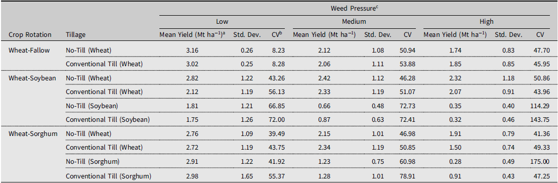
Means of simulated cropping system yields (N = 20 for soybean and sorghum yields, N = 19 for wheat yields)
Notes: Cropping system yields were simulated using ALMANAC (Kiniry et al., Reference Kiniry, Williams, Gassman and Debacke1992).
a One metric ton per hectare is equivalent to approximately 14.87 bushels per acre of wheat and soybean, assuming a 60-pound bushel (Johanns, Reference Johanns2013; North Dakota Wheat Commission, 2022). One metric ton of sorghum per hectare is approximately 15.93 bushels per acre, assuming a 56-pound bushel (Johanns, Reference Johanns2013).
b CV, coefficient of variation.
c Low = 10–20 Palmer amaranth and 5–10 horseweed plants m−2; Medium = 21–30 Palmer amaranth and 11–20 horseweed plants m−2; High = 31–40 Palmer amaranth and 21–30 horseweed plants m−2.
WF and wheat-double crop management schedules followed Decker et al. (Reference Decker, Epplin, Morley and Peeper2009). ALMANAC Management files were modified to reflect different weed management strategies for conventional till and NT systems. Weeds were removed in conventional till systems using a chisel plow. The chisel plow was programmed to reach a depth of 20.34 cm. Tillage operations were assumed to be 90 percent effective in removing weeds (Cahoon, Curran, and Sandy, Reference Cahoon, Curran, Sandy and VanGessel2019). It was also assumed that some weed seeds previously buried at depths where germination was impossible could emerge after tilling (Ball, Reference Ball1992). Specific management tools (chisel plow, disk) were selected and programmed in ALMANAC according to management specifications outlined in Decker et al. (Reference Decker, Epplin, Morley and Peeper2009). A moldboard plow was used to bury annual weed seeds and to control established annuals and seedlings (Cahoon et al., Reference Cahoon, Curran, Sandy and VanGessel2019). A chisel plow is a good option for controlling seedlings and established annuals but a less effective method for burying annual weed seeds (Cahoon et al., Reference Cahoon, Curran, Sandy and VanGessel2019). ALMANAC tillage depths were preprogrammed by ALMANAC staff according to the implement.
Weeds were controlled with herbicides only under NT systems. Herbicide applications were assumed to be 90 percent effective at eliminating weeds, assuming application error and based on estimated weed susceptibility to modes of action (Neve et al., Reference Neve, Diggle, Smith and Powles2003), and for managing weeds on planted sorghum, atrazine and s-metolachlor had ratings of E (“excellent control”; at least 90 percent of Palmer amaranth were controlled) and G (“good control”; between 80 to 90 percent of Palmer amaranth controlled), respectively (Marshall, Reference Marshall2017). Glyphosate and atrazine+s-metolachlor had ratings of E and G-E for managing weeds on planted soybeans, indicating control of at least 80 percent (Hartzler, Reference Hartzler2021). Chlorsulfuron+metsulfuron methyl and pinoxaden had ratings of G and P (“poor control”) for weeds on planted wheat (Neely et al., Reference Neely, Baumann and McGinty2016).
Wheat-fallow system (WF)
Wheat was planted on November 10 and harvested June 15. Diammonium phosphate (18-46-0) and anhydrous ammonia (82-0-0) were applied on October 15 at 109.77 and 30.24 kg ha−1. Top-dress nitrogen (UAN 28%) was applied at 264.36 kg ha−1 on February 10. The seeding rate was 67.21 kilograms of seeds ha−1. Seeds were planted with a seed drill to a soil depth of 40 mm.
Herbicides were applied four times during the NT wheat-fallow rotation, once in June, August, October, and November. Herbicides applied were Axial XL® (wild oat/ryegrass control, 700.25 g ha−1), Finesse® (broadleaf weed control, 17.51 g ha−1), and glyphosate (broadleaf control; applied during the summer as a burndown application on fallow at 1080 g ha−1). Dimethoate was applied to manage insects (876.23 mL ha−1). For conventional till systems, the field was plowed and disked after harvest in June, a second till was performed in August and September, and a final till was performed in October before planting (Decker et al., Reference Decker, Epplin, Morley and Peeper2009; Epplin, Reference Epplin2007).
Wheat-soybean double crop system (WS)
Soybeans were planted on July 10 and harvested on October 20 at a seeding rate of 48.54 kg ha−1. Wheat was planted with a seed drill at a soil depth of 40 mm. Soybeans were planted with a planter, also at a depth of 40 mm. No fertilizer was applied during the soybean cycle. Herbicides were applied four times per year under the wheat-summer crop no-till systems. Bicep Lite II Magnum® (for annual weeds and grasses, 1400.49 g ha−1) and glyphosate (for broadleaf weeds and grasses, 2240.78 g ha−1) were used on soybeans and Axial XL® and Finesse® were used on wheat (the same rate as the WF system). Wheat management followed the same procedures as the WF rotation, except that no summer herbicides or tillage operations were used in the wheat-summer crop management schedules. The field was disked prior to planting soybeans.
Wheat-sorghum double crop (WSrgh)
Sorghum was planted on July 10 and harvested on October 20. Anhydrous ammonia was applied to sorghum on July 1 at 58.61 kg ha−1. The seeding rate was 3.73 kg ha−1. Seeds were planted with a planter at a depth of 40 mm.
Bicep Lite II Magnum® (for broadleaf species and grasses, 2240.78 g ha−1) and Atrazine (broadleaf species, 840.29 g ha−1) were applied to sorghum to control weeds. Sivanto 200 SL® (385.13 g ha−1) was used to protect the crop from insect damage.
Wheat management followed the previous WF rotation management specification, except for summer herbicide applications and tillage. One pre-emergent herbicide and one post-emergent herbicide were applied to double-crop wheat. The field was disked prior to planting sorghum.
Net returns
Yields, crop prices, and input costs were used to calculate each system’s per-hectare net returns (NR). Output prices are from 2020 to match production cost data from the United States Department of Agriculture National Agricultural Statistics Service (USDA-NASS, 2021). Production costs for each cropping system are from the 2020 Oklahoma State University Extension Service Enterprise Budgets (Sahs, Reference Sahs2021). Holding output prices and production costs constant is a simplifying assumption and a limitation of this research. Because prices and costs are constant, producers are assumed to decide on cropping systems based on current price and cost information. While it is likely that price changes and historical prices factor into a producer’s decision-making process, this simplifying assumption isolates the effects of a cropping system on yield while holding prices and costs constant. Net returns for the WF system in period t were calculated as
 $$NR_{WF(t)}=P_{W}\cdot Y_{W\left(t\right)}-\left(C_{W}+C_{F}\right)-R_{C}$$
where P W is the price of wheat ($ Mt−1), Y W(t) is the wheat yield (Mt ha−1), C W is the cost of wheat production ($ ha−1), C F is the cost of field management during the fallow period ($ ha−1), and R C is the per-hectare cropland rental rate for Canadian County, Oklahoma (USDA-NASS, 2021). The cropland rental rate is subtracted from revenue because it is the opportunity cost of not planting a summer crop or renting out the land.
Net returns for a wheat-summer double-crop system in period t were calculated as
 $$NR_{WD(t)}=\left(P_{S}\cdot Y_{S\left(t\right)}+P_{W}\cdot Y_{W(t)}-\left[C_{S}+C_{W}\right]\right)\cdot$$
where P S is the price of the summer crop ($ Mt−1), Y S(t) is the summer crop yield (Mt ha−1), and C S are production costs for the summer crop ($ ha−1). The rental rate (ha−1) was subtracted from wheat-fallow systems to incorporate the opportunity cost of forgoing summer crop production by the landowner or a renting entity. The rental rate (ha−1) was not included in wheat-double crop systems because the field was used to produce a summer crop.
Equipment cost calculations include the use of two tractors. The 95-horsepower tractor was used to fertilize, plant, and apply herbicides and pesticides. The 160-horsepower tractor was used for conventional till operations. The certified wheat seed cost was $0.42 kg−1 ($28.40 ha−1) for wheat production in all systems. Certified seeds are more expensive than uncertified seeds due to the extra costs of cleaning seeds.
Manufacturer-recommended rates were programmed into ALMANAC’s management files to control weeds. Herbicides and pesticides included in wheat budgets were Axial XL® ($0.04 g−1) ($29.39 ha−1), Finesse® ($0.58 g−1) ($10.18 ha−1), and dimethoate ($0.009 mL−1) ($8.12 ha−1). Anhydrous ammonia (82-0-0) ($0.53 kg−1) ($16.00 ha−1), diammonium phosphate (18-46-0) ($0.42 kg−1) ($45.98 ha−1), and 28% urea ammonium nitrate ($0.26 kg−1) ($69.94 ha−1) were used to fertilize wheat. Total fuel, lubrication, and repair costs for conventional till and NT wheat were $140.42 and $78.10 ha−1, respectively.
Soybean and sorghum seed were $2.25 and $8.06 kg−1, respectively ($109.06 ha−1 for soybean seed, $30.10 ha−1 for sorghum seed). Sorghum seed was treated with Gaucho® to protect against chinch bugs. Anhydrous ammonia (82-0-0) was used to fertilize sorghum at $0.53 per kilogram ($31.01 ha−1). Bicep Lite II Magnum® ($0.03 g−1) ($37.94 ha−1), Atrazine ($0.004 g−1) ($3.56 ha−1), and Sivanto 200 SL® ($0.09 g−1) ($34.37 ha−1) were used on sorghum to control for weeds and insects, respectively. Bicep Lite II Magnum® ($0.03 g−1) ($47.86 ha−1) and glyphosate ($0.005 g−1) ($5.33 ha−1) were used on soybeans to control weeds. Total fuel, lubrication, and repair costs were $61.90 ha−1 for NT soybean and $102.53 ha−1 for NT sorghum. Total fuel, lubrication, and repair costs for conventional till soybean and sorghum were $97.52 and $133.65 ha−1, respectively.
Comparison of cropping system yield performance and net returns
Net returns and yield performance of cropping systems are analyzed graphically and empirically. A two-sample Kolmogorov-Smirnov (KS) test is used to determine if each production system’s yields and net return distributions were different (Kolmogorov, Reference Kolmogorov1933; Smirnov, Reference Smirnov1939). The null hypothesis is that the two distributions are indistinguishable. The p-value associated with each pairwise comparison is used to determine if the null hypothesis is rejected. KS tests were performed using the ks.test function of the stats package in Rstudio (v. 2.1.461) (RStudio Team, 2020).
Stochastic dominance (SD, Anderson, Reference Anderson1974; Mas-Colell et al., Reference Mas-Colell, Whinston and Green1995) was used to determine if risk preferences affected the decision to use a particular cropping system. SD analysis uses two criteria to compare challenger and defender technologies: (1) First-degree stochastic dominance (FDSD) and (2) second-degree stochastic dominance (SDSD). The first criterion assumes that producers generally prefer higher to lower returns. The second criterion assumes that risk-averse producers prefer to avoid low-valued outcomes but tolerate upside variability in net returns (Lambert and Lowenberg-DeBoer, Reference Lambert and Lowenberg-DeBoer2003). In the generic case of any generic expected utility (EU) function, FDSD implies that the utility function is monotonically increasing (u′(x)> 0) in net returns, meaning that individuals prefer more to less. SDSD implies that the second derivative of a generic EU function is decreasing (u″(x)<0) and monotonically increasing implies risk aversion (Dillon and Anderson, Reference Dillon and Anderson1990).
Graphically, FDSD occurs when a challenger’s empirical cumulative density function (ECDF) of net returns is always to the right of a defender technology. The second assumption – that people prefer to avoid variability in low net returns but tolerate upside variability – characterizes SDSD. Graphically, the empirical distributions of net returns from competing technologies cross at least once. A challenger with the lowest net return can never FDSD- or SDSD-dominate a defender. However, suppose the total area of the crossover areas for a challenger with a larger minimum net return exceeds the total area of crossover areas favoring a defender. In that case, the challenger dominates the defender by the second-degree criterion. The stochastic dominance analysis was conducted using a spreadsheet created by Lowenberg-DeBoer et al. (Reference Lowenberg-DeBoer, Krause, Deuson and Reddy1990) and Hien (Reference Hien1997). In FDSD and SDSD, a prevailing practice consistently yields a higher average return.
The stochastic dominance (SD) framework was used in this analysis because, unlike the stochastic efficiency (SE) framework (Hardaker et al., Reference Hardaker, Lien, Anderson and Huirne2015), SD requires fewer assumptions about risk preferences; namely, choosing an expected utility function and risk aversion parameter is not required. The rankings identified by SD are driven by the data and not necessarily by the expected utility function selected. SD ranks a set of actions or technologies by progressively comparing one alternative to the next until all comparisons are completed (Anderson, Reference Anderson1974). An ordering of FDSD or SDSD technologies remains, including indeterminate cases where neither FDSD nor SDSD can be established.
Sensitivity: cropping systems and weed pressure
A cost-to-go dynamic programming (DP) procedure (Bertsekas, Reference Bertsekas2000) is used to determine which cropping system maximizes net returns over a planning horizon. Earlier applications of cost-to-go programming include Burt and Allison (Reference Burt and Allison1963)’s study of rainfed WF systems in Kansas. Similar DP applications have examined state-contingent optimal cropping strategies (El-Nazer and McCarl, Reference El-Nazer and McCarl1986; Farquharson et al., Reference Farquharson, Cacho, Mullen and Schwenke2008; Jones et al., Reference Jones, Cacho and Sinden2006; Livingston et al., Reference Livingston, Fenandez-Cornejo, Unger, Osteen, Schimmelpfennig, Park and Lambert2015; Patino et al., Reference Patino, Pucheta, Fullana, Schugurensky and Kuchen2004; Periera et al., Reference Periera, Fontes, Ferriera, Pinho, Oliveira, Costa and Silva2013; Tongtiegang et al., Reference Tongtiegang, Zhao, Lei, Wang and Wu2017; Van Kooten et al., Reference Van Kooten, Weisensel and Chinthammit1990). Optimal policies are determined by choosing a cropping system that maximizes the sum of discounted net returns over each weed density state, measured as plants m−2.
A producer maximizes the expected present value of net returns ha−1 by choosing a cropping system conditional on some level of observed weed pressure and on the tillage method employed. The system used by the producer impacts weed pressure. For example, some practices may be more effective in controlling weed seed banks over multiple periods than others. The producer’s control variable is the cropping system j= WF, WS, or WSrgh. These systems are evaluated separately for conventional till and NT systems, assuming that a producer would unlikely switch back and forth between either tillage method from one season to the next. Some NT farmers might switch to conventional tillage to manage weeds. Zhou et al. (Reference Zhou, Roberts, Larson, Lambert, English, Mishra, Falconer, Hogan, Johnson and Reeves2016) found this to be the case for a limited number of cotton producers. Tillage methods are indexed by k = NT, conventional till. Stages, or periods, are years and denoted as t = 1, 2, …T. The state variable is the level of weed pressure and indexed as i = low (“L”), medium (“M”), and high (“H”). Details explaining these categories and the likelihood of their occurrence follow in the “Weed Pressure Transition Probabilities” section (below).
Net returns for wheat-double-crop systems in period t are the sum of the winter wheat and summer crop net returns. For the WF system, period net returns are from winter wheat less the costs of managing the field during the summer months (e.g., chiseling and herbicide applications) and the opportunity cost of renting the land ($ ha−1). Expected (average) net returns from a system are used for comparisons, which means we assume that a producer makes decisions based on expected yields and prices. The expected net return associated with each crop decision (j), tillage type (k), and state i is π jik (Table 2).
Net returns, simulated cropping system and weed pressure ($ ha−1)
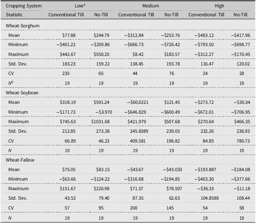
Notes: Yields used to generate net returns were simulated using ALMANAC (Kiniry et al., Reference Kiniry, Williams, Gassman and Debacke1992). CV, coefficient of variation; Std. Dev., standard deviation.
a Low = 10–20 Palmer amaranth and 5–10 horseweed plants m−2; Medium = 21–30 Palmer amaranth and 11–20 horseweed plants m−2; High = 31–40 Palmer amaranth and 21–30 horseweed plants m−2.
b N = simulated periods.
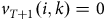
An optimal policy determines which cropping system maximizes the sum of expected net present values of returns, conditional on a weed pressure state. Bellman (Reference Bellman1957)’s return function is maximized to determine the sum of expected net returns over a T-period planning horizon. Let v t (i) denote the discounted expected return for a t-period decision sequence under state i. The return function is $v_{T}(i,k)=\max _{j\in (\mathit{WF},\mathit{WS},\mathit{WSrgh})} \{\pi _{j}^{ik}+\delta \cdot \sum _{i'=1}^{M}p_{ii'}^{jk}\cdot v_{T-1}(i)\}$
, subject to
$v_{T}(i,k)=\max _{j\in (\mathit{WF},\mathit{WS},\mathit{WSrgh})} \{\pi _{j}^{ik}+\delta \cdot \sum _{i'=1}^{M}p_{ii'}^{jk}\cdot v_{T-1}(i)\}$
, subject to
 $$v_{T+1}\left(i,k\right)=0$$
where t = 0, …, T; i = low, medium, high, i′ aliases i, indexes weed pressure states; and [ $p_{ii'}^{jk}$
] is a matrix of transition probabilities governing the likelihood that weed pressure will increase or decrease from one period to the next (discussed below). The discount factor is δ and is calculated as one divided by one plus the interest rate. The interest rate is 1.44 percent, the 2020 average long-term US bond interest rate (OECD, 2022). The discount factor represents the producer’s preference to enjoy net returns sooner rather than later. The constraint is a terminal condition and implies that the value function is zero in the final period (that is, returns are zero once farming the field ends). Equation 1 was solved using Miranda and Fackler (Reference Miranda and Fackler2004)’s ddpsolve package (Miranda and Fackler, Reference Miranda and Fackler2004) in MATLAB (R2020a, Update 7; MathWorks Inc., 2020).
$p_{ii'}^{jk}$
] is a matrix of transition probabilities governing the likelihood that weed pressure will increase or decrease from one period to the next (discussed below). The discount factor is δ and is calculated as one divided by one plus the interest rate. The interest rate is 1.44 percent, the 2020 average long-term US bond interest rate (OECD, 2022). The discount factor represents the producer’s preference to enjoy net returns sooner rather than later. The constraint is a terminal condition and implies that the value function is zero in the final period (that is, returns are zero once farming the field ends). Equation 1 was solved using Miranda and Fackler (Reference Miranda and Fackler2004)’s ddpsolve package (Miranda and Fackler, Reference Miranda and Fackler2004) in MATLAB (R2020a, Update 7; MathWorks Inc., 2020).
Weed pressure transition probabilities
Transition probabilities govern the evolution of weed pressure from state i to i′ between periods, given the implementation of the (j, k)th cropping system. Each cropping system and conventional till-NT tillage method has a unique transition probability matrix (six matrices). Weed density is observed at the beginning of a planting cycle (fall) in state i = low (“L”), medium (“M”), and high (“H”). Weed density levels were discretized by calculating the number of weeds m−2 from ALAMANAC output and then categorizing the counts into discrete groups based on classifications reported in the literature (Crose et al., Reference Crose, Manuchehri and Baughman2020; Mahoney et al., Reference Mahoney, Jordan, Hare, Leon, Roma-Burgos, Vann, Jennings, Everman and Cahoon2021; Shyam et al., Reference Shyam, Chahal, Jhala and Jugulam2020; Swanton et al., Reference Swanton, Shrestha, Clements, Booth and Chandler2002; Van De Stroet and Clay, Reference Van De Stroet and Clay2019). Under the low weed pressure state, the number of horseweed and Palmer amaranth plants m−2 were five to 10 and 10 to 20, respectively. Weed counts m−2 for the medium density state was 11 to 20 and 21 to 30 plants m−2 for horseweed and Palmer amaranth, respectively. High weed pressure counts were 21 to 30 and 31 to 40 plants m−2, respectively, for horseweed and Palmer amaranth.
Weed biomass at wheat planting was used to benchmark the weed pressure categories. Cumulative horseweed and Palmer amaranth biomass were recorded at wheat harvest and converted to plants m−2. Palmer amaranth biomass was assumed to be 35 g plant−1 (Mahoney et al., Reference Mahoney, Jordan, Hare, Leon, Roma-Burgos, Vann, Jennings, Everman and Cahoon2021). Horseweed biomass was assumed to be 4.3 g plant−1 (Nandula et al., Reference Nandula, Poston, Kroger, Reddy and Reddy2015). Weeds m−2 counts were then assigned to L, M, or H states. Each system had 20 weed biomass measurements, one for each simulation year.
Transition probabilities were estimated using a maximum likelihood procedure (Amemiya, Reference Amemiya1985), which yields a closed-form solution for each probability:
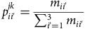 $$p_{ii'}^{jk}={m_{ii'} \over \sum _{i'=1}^{3}m_{ii'}}$$
where m ii′ is the number of times over the 20 periods that weed pressure was observed in state i, period t, and was followed by the weed pressure moving to state i′ in time t+ 1. Transition probabilities were estimated using the markovchain package (Spedicato, Reference Spedicato2017) in RStudio (v.1.4.1106; RStudio Team, 2020).
As the number of periods increases, the transition probabilities converge to a stationary distribution (Isaacson and Madsen, Reference Isaacson and Madsen1976). In other words, in the long term and no matter what the beginning state is, steady-state transition probabilities proxy the proportion of time the system will be observed in state i as π
i
. The stationary distribution of transition probability matrix ${\bf P}$
is some vector
${\bf P}$
is some vector ${\bf \pi\ }$
such that
${\bf \pi\ }$
such that ${\bf P'}{\bf \pi\ }={\bf \pi }$
. The vector
${\bf P'}{\bf \pi\ }={\bf \pi }$
. The vector ${\bf \pi\ }$
is constant for all states and implies that, over the longer term, no matter what state of weed pressure the cropping area started in, the proportion of time the cropping area spends in weed pressure state i is approximately π
i
for all i. Steady-state transition probabilities were solved as a system of linear equations using Miranda and Fackler (Reference Miranda and Fackler2004)’s procedure.
${\bf \pi\ }$
is constant for all states and implies that, over the longer term, no matter what state of weed pressure the cropping area started in, the proportion of time the cropping area spends in weed pressure state i is approximately π
i
for all i. Steady-state transition probabilities were solved as a system of linear equations using Miranda and Fackler (Reference Miranda and Fackler2004)’s procedure.
A drawback of using the transition probabilities in Eq. 4 is that weed pressure transitions are assumed to be constant over time. This is a simplifying assumption. Weed populations have variable lifecycles. The transition probabilities could differ between older weed populations with a higher probability of natural die-offs and newly established populations (Torell et al., Reference Torell, McDaniel and Williams1992). Information regarding the age of the weed population at the time of biomass measurement was unavailable, and this simplifying assumption is a caveat.
Medium- and long-term net returns
Net returns from each system are calculated for medium- and long-term planning horizons. The medium-term evaluation is a five-year planning horizon. There is no terminal value for the long-term planning horizon (e.g., equation 2 is omitted), and land used to produce crops is assumed to continue indefinitely. Burt and Allison (Reference Burt and Allison1963) and Kennedy (Reference Kennedy1986) show that, as the number of periods in a planning horizon increases, the recurrence relation of Eq. 1 converges to an invariant decision rule according to the properties of Markov systems. In the long term, an optimal policy corresponding with a specific weed pressure state is invariant no matter the period. Thus, for a long-term planning horizon, whenever a producer observes weed pressure state i before planting wheat, the optimal decision rule is to implement cropping system j.
Backward induction cannot be used to solve infinite-horizon weed management scenarios. An approximation method is required to find an optimal policy that maximizes discounted net returns. A policy iteration procedure is used here, which solves optimal cropping systems, given a prevailing state of weed pressure (Miranda and Fackler, Reference Miranda and Fackler2004).
Sensitivity: net returns, weed pressure dynamics, and stochastic yields
Monte Carlo methods were used to evaluate the performance of each system under yield uncertainty. The Monte Carlo simulation included the following steps for m = 1,…M iterations. First, the means and variances of each ALMANAC-simulated crop yield a = W, Soy, Srgh, for cropping system j= WF, WS, and WSrgh and tillage method k= conventional till and NT under weed pressure i= L, M, and H were calculated as ${\hat u_{ia\left( j \right)k}}$
and
${\hat u_{ia\left( j \right)k}}$
and $\hat\sigma _{ia\left( j \right)k}^2$
, respectively. Afterward:
$\hat\sigma _{ia\left( j \right)k}^2$
, respectively. Afterward:
-
1. Yields from each cropping system were randomly drawn from a truncated normal distribution, $Y_{ia\left( j \right)k}^m \sim N\left( {{{\hat \mu }_{ia\left( j \right)k}},\hat \sigma _{ia\left( j \right)k}^2} \right);Y_{ij\left( a \right)k}^* \in {{\mathbb R}^ + }$
.
$Y_{ia\left( j \right)k}^m \sim N\left( {{{\hat \mu }_{ia\left( j \right)k}},\hat \sigma _{ia\left( j \right)k}^2} \right);Y_{ij\left( a \right)k}^* \in {{\mathbb R}^ + }$
. -
2. Randomly drawn yields,
$Y_{ia\left( j \right)k}^m$
, were used to re-calculate net returns for each cropping/tillage system and weed pressure state (denoted as
$\hat \pi _{ijk}^m$
). -
3. Equation 1 was re-solved, given
$\hat \pi _{ijk}^m$
. -
4. Optimal cropping decisions under each weed pressure state were recorded as a (0,1) variable at each iteration. For example, if NT-WF net returns were optimal under weed pressure state L, then “1” was recorded for NT-WF, and “0” was assigned to challengers.
-
5. The probability that a cropping system was profitable under each state is the sum of the (0,1) outcomes divided by M = 1,000 iterations. For example, suppose NT-WF net returns were optimal 200 times when the weed pressure state was low. In that case, there is a 0.20 likelihood that this system generated the highest net returns, given stochastic yields and the weed pressure state.


Results
Cropping system yields
The results section is structured as follows: Cropping system simulations are compared with observed yields. Following this, net returns and yields are compared across different weed density levels using both summary statistics and stochastic dominance analysis. Subsequently, transition probability estimates are discussed, which is followed by the medium- and long-term results of dynamic optimization. Finally, results from the medium- and long-term dynamic optimization with uncertainty are discussed.
Comparing simulated cropping system yields with observed yields is crucial because simulated yields are derived from mathematical models representing different agricultural processes. This comparison serves as means to validate the simulated data.
Average yields generated under the low weed density scenario were used to compare system performance with observed crop yield data (Table 1). Soybean and sorghum did not perform well during the 2020 El Reno field trials. Experimental data for sorghum and soybean yields averaged less than 0.001 Mt ha−1. Therefore, sorghum and soybean yields from the National Agricultural Statistics Service (NASS), 1990 to 2020 in Canadian County, Oklahoma, were used to calculate soybean and sorghum yields (USDA-NASS, 2021). The average sorghum yield from NASS was 3.08 Mt ha−1. The NASS soybean average yield for the same period was 1.60 Mt ha−1. These values were used to benchmark ALMANAC’s crop growth modules for these crops. Sorghum and soybean yields generated by ALMANAC were 2.94 (WSrgh-NT and -conventional till average yield) and 1.78 (WS-NT and conventional till average yield) Mt ha−1, respectively.
Simulated wheat yields were compared to the experimental trial data and the NASS wheat yield data for the location and period listed above. The observed wheat yield average from the experimental plots for WF systems was 3.85 Mt ha−1. The average wheat yield for Canadian County was 2.30 Mt ha−1 (USDA-NASS, 2023). Simulated WF wheat yields were 3.09 Mt ha−1 (WF-NT and -conventional till average yield). The difference between simulated and observed wheat yield averages may be attributable to assumptions about tillage and herbicide effectiveness. The notable difference between the average wheat yield from NASS and the simulated wheat yield average from ALMANAC may also be due to the management practices recommended for the region (for example, fertilizer types and rates and seeding rates). In addition, average yields from NASS may not have been obtainable under the same assumptions used in the crop growth model. The average yield for wheat followed by a summer crop was 2.83 and 2.53 Mt ha−1 for WS and WSrgh systems in the trial plots, respectively. Simulated WS and WSrgh wheat yields were 2.47 and 2.74 Mt ha−1, respectively.
Low weed pressure
Average wheat yields ranged from 2.12 to 3.16 Mt ha−1 (WF-NT) (Table 1). Average soybean yields were higher for NT systems. In comparison, average sorghum yields were higher for conventional till systems.
Moderate weed pressure
Average wheat yields ranged from 2.06 (WF-conventional till) to 2.42 Mt ha−1 (WS-NT) (Table 1). Average soybean yield ranged from 0.66 (NT) to 0.87 Mt ha−1 (conventional till). Average sorghum yields ranged from 1.23 (NT) to 1.28 Mt ha−1 (conventional till) (Table 1).
High weed pressure
Wheat yields ranged from 1.50 (WSrgh-conventional till) to 2.32 Mt ha−1 (WS-NT) (Table 1). The highest average soybean yield was observed in an NT system. The highest average sorghum yield occurred in a conventional till system (Table 1).
It is worth noting the variation in yield damage caused by weed pressure across different crops. Among the cropping systems simulated, summer crops tend to experience more significant damage from weed pressure compared to wheat crops. According to research by Flessner et al. (Reference Flessner, Burke, Dille, Everman, VanGessel, Tidemann, Manuchehri, Soltani and Sikkema2021), winter wheat typically faces yield losses ranging from 0.3 to 48 percent due to broadleaf weeds. In contrast, soybeans can suffer yield losses of 17 to 79 percent due to Palmer amaranth, and sorghum may experience losses of 38 to 63 percent from the same weed species, as reported by Ward and Webster (Reference Ward and Webster2013). These studies suggest that weed pressure has a comparatively lesser impact on winter wheat compared to sorghum and soybeans. It is also worth noting that Palmer amaranth has been observed to overcome cultural weed management practices, including crop rotation (Crow et al., Reference Crow, Steckel, Hayes and Mueller2015). However, horseweed can be effectively controlled through tillage and crop rotations, as indicated by Shaner et al. (Reference Shaner, Lindenmeyer and Ostlie2013). Therefore, it is more likely that summer crops will suffer greater damage from weed pressure compared to wheat crops.
Net returns
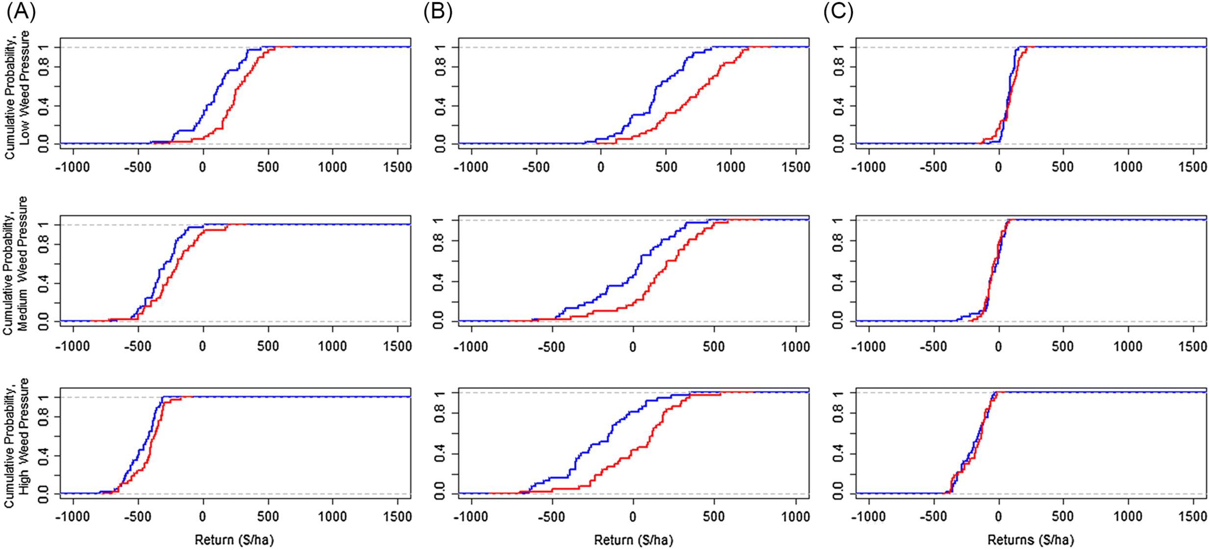
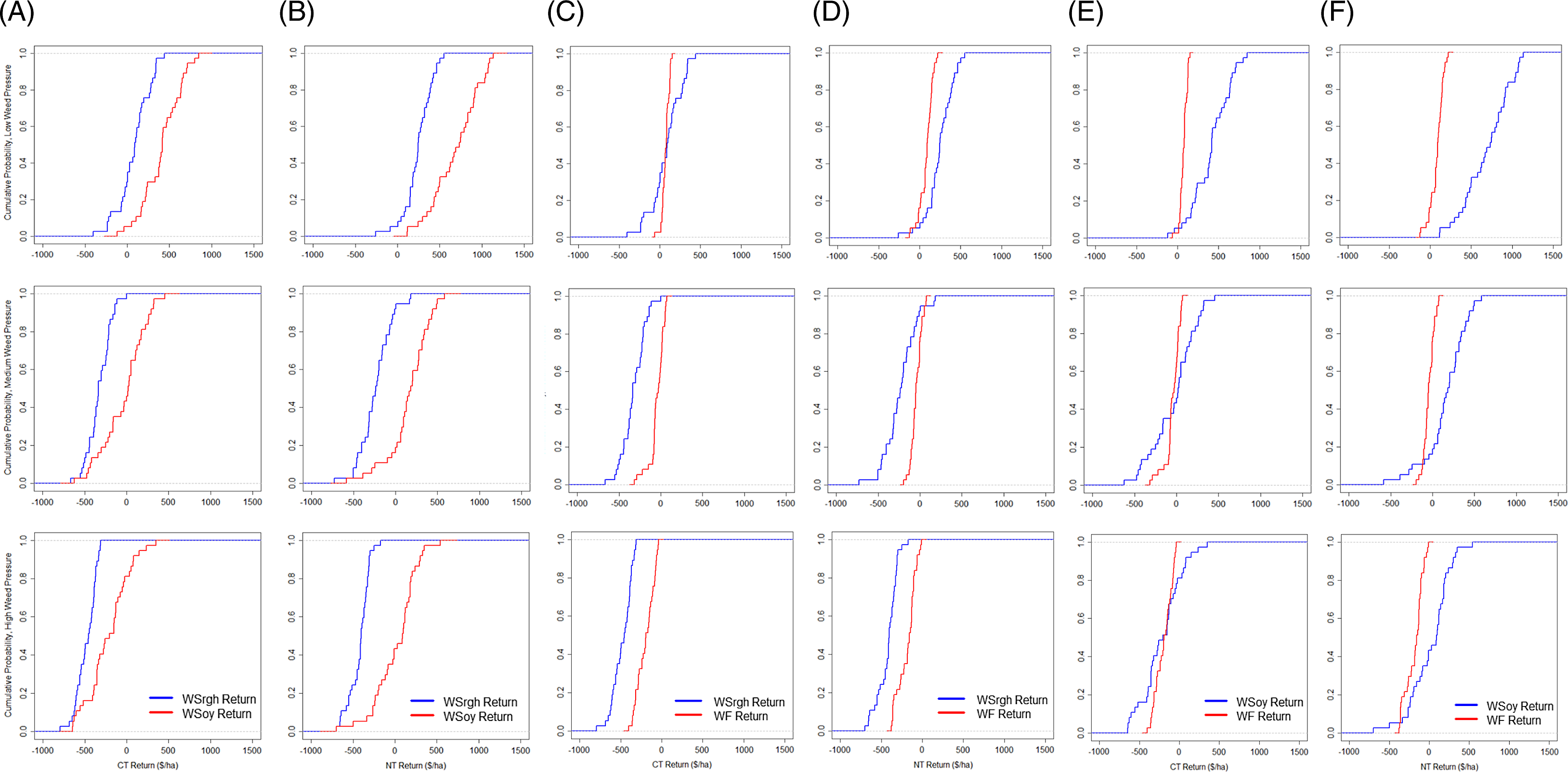
All systems’ average net returns were positive when weed pressure was low but were negative at higher levels of weed pressure (Table 2). Figures 1 and 2 show each system’s ECDFs. The net return ECDFs indicate the performance of each system under different growing conditions. Lower yield outcomes presumably occur when growing conditions are unfavorable (e.g., hot, drier conditions), which decreases net returns.
Pairwise comparisons of wheat-sorghum (Panel A), wheat-soybean (Panel B), and wheat-fallow (Panel C) net returns within system and weed pressure by tillage practice.
Notes: CT and NT denote conventional till and no-till, respectively.
Pairwise comparisons of WSrgh and WS (CT– Panel A, NT – Panel B), WSrgh and WF (CT– Panel C, NT – Panel D), and WS and WF (CT – Panel E, NT – Panel F) net returns by system within tillage practice and weed pressure.
Notes: CT and NT denote conventional till and no-till, respectively. WF, WS, and Wsrgh denote wheat-fallow, wheat-soybean, and wheat-sorghum systems, respectively.
Low weed pressure
Average net returns ha−1 were highest for WS, WSrgh, and WF systems under NT (Table 2). WF returns were negative at the 3rd (conventional till) and 16th (NT) percentiles of its empirical distributions (Table 3). Average net returns ha−1 for NT were more likely to exceed conventional till net returns as growing conditions improved, as demonstrated by the intersection at the 25th percentile of NT- and conventional till-WF distributions (Panel C, Fig 1). WSrgh systems had a greater likelihood of generating higher net returns ha−1 compared to WF systems under moderate and excellent growing conditions when weed pressure was low (40th percentile (conventional till-WF/WSrgh), 5th (NT-WF/WSrgh)) (Panels C and D, Fig 2).
Cumulative probabilities associated with cropping system net returns by system, tillage, and weed pressure
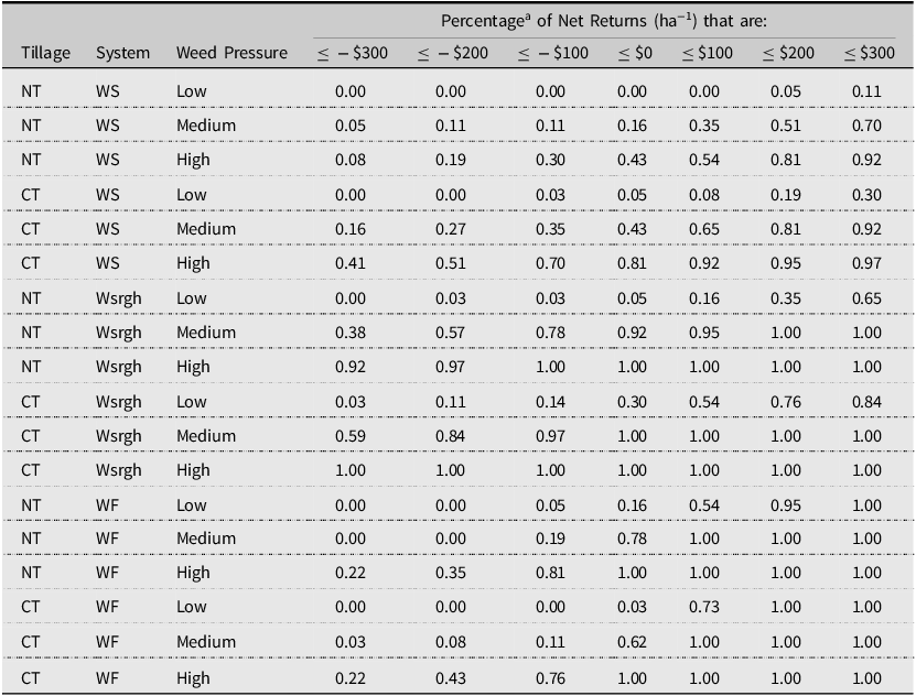
Notes: WF, WS, and Wsrgh denote wheat-fallow, wheat-soybean, and wheat-sorghum systems, respectively. NT and CT denote no-till and conventional tillage practices, respectively. There were 19 observations used for wheat-soybean and wheat-sorghum systems and 19 observations used for wheat-fallow systems. Cropping systems were simulated using ALMANAC (Kiniry et al., Reference Kiniry, Williams, Gassman and Debacke1992).
A higher percentage of net returns were negative for conventional till/NT-WSrgh systems compared to WS systems (Table 3). WS systems were likelier to perform better under all growing conditions when weed pressure was low than WSrgh systems (Panels A and B, Fig 2).
Statistical differences in net returns were observed between conventional till and NT WS systems (KS test, p < 0.001) (Table 4). The NT-WS system FDSD and SDSD dominated the conventional till-WS system. Hence, risk-neutral and risk-averse producers would favor NT-WS systems over conventional till-WS systems. Additionally, WS systems outperformed WSrgh systems in both types of tillage when assessed by FDSD and SDSD. These rankings suggest that risk-neutral and risk-averse producers would choose WS systems over WSrgh systems, regardless of the tillage practice used. There were statistically significant differences in net returns between WF and NT/conventional till-WS systems (KS-test, p = 0.001 (NT), 0.001 (conventional till)) and NT/conventional till-WSrgh systems (KS-test, p = 0.009 (CT); p = 0.001 (NT)).
Stochastic dominance analysis of cropping system net returns ha−1
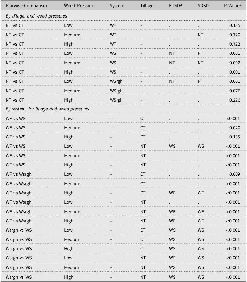
a A “.” in a column means that neither system was FDSD or SDSD.
b The P-value is calculated for the Kolmogorov–Smirnov pairwise tests. The null hypothesis is that the distributions are not different.
Notes: Table 4 corresponds to Figures 1 and 2. NT and CT denote no-till and conventional tillage practices. WF, WS, and Wsrgh denote wheat-fallow, wheat-soybean, and wheat-sorghum systems, respectively. There were 20 observations of wheat-fallow net returns and 19 observations of wheat-soybean and wheat-sorghum. FDSD and SDSD denote first-degree stochastic dominance and second-degree stochastic dominance, respectively.
Moderate weed pressure
NT systems generated higher net returns across all crop rotations (Table 2). In conventional till and NT systems, the WS system outperformed the WSrgh system. WSrgh systems generated higher average net returns ha−1 under NT than conventional till (Table 2).
NT-WSrgh net returns turned negative at the 92nd percentile (Table 3). All conventional till-Wsrgh net returns were negative. Conventional till-WS and NT-WS net returns were negative up to the 43rd and 16th percentile, respectively. Conventional till-WF and NT-WF net returns were negative at their respective 62nd and 78th percentile distributions. When weed pressure was moderate, the WSrgh-conventional till systems were more likely to generate higher net returns ha−1 (than Wsrgh-NT) when growing conditions were extremely poor, as shown by the intersection of NT- and conventional till-Wsrgh CDFs at the 5th percentile (Panel A, Fig 1). The likelihood of NT-WS net returns exceeding conventional till-WS returns was consistently higher in all growing conditions (Panel B, Fig 1).
The NT-WF system dominated NT-WSrgh by the FDSD and SDSD rules, and were also significantly different (Table 4). The NT system dominated conventional till by the FDSD and SDSD criteria for the WS rotation (Table 4). Risk-neutral and risk-averse producers would prefer using NT for a WS system. NT practices dominated conventional till by SDSD in the WF system (Table 4). Research finds that well-performing herbicides can effectively replace tillage operations, assuming that targeted weeds are susceptible to the herbicide (Wicks et al., Reference Wicks, Smika and Hergert1988). Therefore, NT’s dominance over conventional till might change if herbicide resistance was modeled.
High weed pressure
In NT systems, WS net returns were comparatively higher than the other technologies but were still negative. The WF system performed better than WS and WSrgh under conventional till. The WSrgh system performed better under NT than conventional till. All WF and WSrgh net returns were negative (Table 3). NT- and conventional till-WS generated negative net returns at the 43rd and 81st percentile, respectively (Table 3).
The WF system dominated WSrgh by FDSD and SDSD under NT and conventional till (Table 4). Conventional till/NT-WF and WSrgh net returns were also statistically different, as were NT-WF and NT-WS net returns. The WF system generated higher returns under conventional till and NT practices than WSrgh systems. For the WS system, NT and conventional-till net returns were statistically different for the WS system at the 1-percent significance level (KS-test, p = 0.001, Table 4).
Cropping systems and weed pressure dynamics
Transition probabilities
The rows in Table 5 denote weed density in period t. The columns denote weed density at t + 1. For example, suppose weed pressure was moderate in period t and the producer used a WF-conventional till system (Row 2, Table 5). In that case, there is a 0.38 probability that the cropping area will transition to a low weed density state by the next period. If a cropping area is in a medium weed pressure state, the tendency is that pressure will remain medium. An absorbing state was identified for conventional till wheat-sorghum and wheat-soybean systems, as evidenced by the transition probability of “1”. The implications for a farmer are that if a conventional till wheat-sorghum (conventional till wheat-soybean) system is always used, then within nine years (five years), the producer will end up always managing a medium-density weed population of horseweed or Palmer amaranth. Intraspecific competition between weeds and continuous crop-weed competition lowers the probability of weed pressure remaining in a high-pressure state because of carrying capacity constraints and increased pressure on weed populations through more intensive management. When weed pressure is low, the most likely outcome is that the pressure will transition to a high-pressure state. This transition is likely because horseweed and Palmer amaranth are prolific seed producers. Given the weed control methods considered here, weed pressure in all cropping systems tended toward a medium pressure state in the longer term.

Steady-state transition probabilities were calculated to determine the frequency at which a cropping area would be observed in a low, medium, or high state of weed pressure in the longer term. For example, it would be expected that, on average, the likelihood a producer would observe a low weed pressure state before planting is 0.21, given that a conventional till-WF system was implemented (Table 5, Row 1, Column 6). Conventional till-WF and conventional till-WS reached their steady-state probability distributions after five periods, while the WSrgh system reached its steady-state distribution in nine periods. NT-WF and NT-WSrgh systems achieved steady-state distributions in four periods, but the NT-WS systems still required five years. These differences suggest that NT-WF and NT-WSrgh are relatively more stable (i.e., the steady state is reached more quickly) regarding weed density and subsequent net returns than the other systems. NT-WF and NT-WSrgh reach their stationary probability distributions sooner than the other systems. The similarity of steps required to reach a steady state among NT/conventional till-WF and NT/conventional till-WS systems suggests that tillage activities are not as impactful on the stability of weed pressure relative to tillage activities in conventional till/NT-Wsrgh systems. The similarity between NT and conventional till weed pressure transition probabilities in WF systems suggests that weed pressure dynamics vary little between practices. Therefore, no single tillage system appears to control better weed pressure dynamics in WF systems. Weed pressure did not differ significantly between tillage systems in the longer term; therefore, tillage systems should not be selected based on weed pressure management ability alone. Because weed pressure tends to a medium-density level regardless of the tillage system, decisions regarding tillage systems should include other components such as control costs.
Medium-term optimal cropping systems
Table 6 summarizes optimal cropping systems within a medium-term planning horizon, employing a combination of current price and average yield optimization alongside a Monte-Carlo analysis for both conventional-till and NT systems. Columns two to six represent the findings for conventional-till systems. In contrast, columns seven to eleven illustrate the results for NT systems. Columns two and seven present optimization outcomes with fixed prices and yields which resulted in the selection of a single optimal system. Conversely, columns three through five (conventional till) and eight through ten (NT) include the results from the Monte-Carlo analysis which are percentages of Monte-Carlo iterations each cropping system was identified as optimal.
Optimal cropping systems assuming a 1.44% discount rate and a medium-term planning horizon
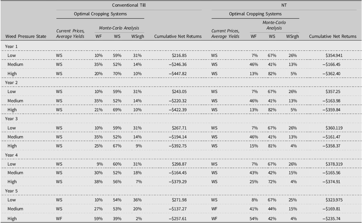
Notes: WS denotes a wheat-soybean system, WSrgh a wheat-sorghum system, and WF a wheat-fallow system. NT denotes no-till operations. 1000 Monte Carlo iterations were performed.
A five-year planning horizon was used to determine which system generated the highest net returns for the medium term. Risk-neutral producers would implement WS systems in the first four years under all states of weed pressure and conventional till and NT tillage systems (Table 6). In the final year of the planning horizon, risk-neutral producers using conventional till systems would switch to a WF system when weed pressure is high. Profit-maximizing producers using NT would select WF systems in year five’s medium and high weed pressure scenarios. The switch from WS to WF occurs because the producer makes no returns after the final year due to the terminal condition of Eq. 2 and because weed control costs for WF systems are lower.
Cumulative discounted net returns ha-1 were positive for the low weed pressure scenario for all years and highest under NT practices (Table 6). Conventional till systems generated negative but higher net returns under medium weed pressure, while NT systems generated higher net returns under high weed pressure. NT yields were generally higher than conventional till yields for nearly all crops and weed pressure states when weeds are in medium and high, but conventional tillage systems sometimes better clear the field of weeds before planting.
Sensitivity: medium term
For conventional till practices and low weed pressure, given stochastic yields, WS systems net returns ha−1 were higher than net returns from the competing systems for 59 conventional till, years 1–3) and 67 (NT, periods 1–5) percent of the 1,000 Monte Carlo simulations (Table 6). In years four and five, there was a 0.60 and 0.54 probability that conventional till-WS systems generated the highest net returns compared to challengers, respectively. WSrgh systems generated the highest net returns for 31 percent of simulations when weed pressure was low and conventional till was implemented (31 to 36 percent). When NT practices were implemented, and weed pressure was low, WSrgh systems generated the highest net returns for 26 percent of simulations. NT- and conventional till-WF systems had the lowest likelihood of generating the highest net returns compared to challengers when weed pressure was low (range: 7 to 10 percent).
The likelihood that WF systems generated the highest net returns increased as weed pressure increased. When weed pressure was moderate, WF systems had a 0.35 probability of producing the highest net returns under conventional till practices in year one. This probability decreased to 0.27 probability in year five. For NT-WF systems, the likelihood of the highest returns occurring under the NT-WF systems decreased from 46 percent in year one to 41 percent in year five. When weed pressure was moderate, the WS systems were most likely to generate higher net returns than the alternative systems under conventional till. When weed pressure was high, conventional till-WS and NT-WS systems were more likely to generate the highest net returns for the first four years of the planning horizon. In the final year, when weed pressure was high, WF systems were most likely to generate the highest net returns under conventional till (59 percent) and NT (54 percent). WSrgh systems had the lowest likelihood of beating challenger systems under both types of tillage, all years, under medium and high weed pressure.
Long-term optimal cropping systems
A risk-neutral producer would implement WS systems under all weed pressure levels and conventional till and NT tillage practices over an infinite-planning horizon (Table 7). For all cropping systems and weed pressure states, cumulative discounted net returns ha−1 were higher for NT systems than conventional till. The most considerable difference in cumulative net returns occurred in the high weed pressure state. NT cumulative net returns were approximately $1,500 ha−1 greater than cumulative net returns from conventional till systems. For a long-term planning horizon, the optimal conventional till and NT systems agree with the system ranking found for the first four periods of the shorter planning scenario.
Optimal cropping systems and Monte Carlo analysis results by weed density state, assuming a long-term planning horizon
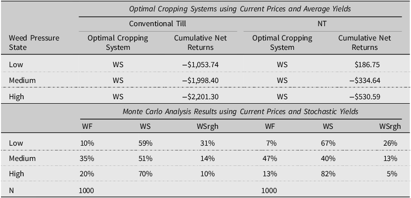
Notes: NT denotes no-till. N denotes the number of Monte Carlo iterations.
Sensitivity: long-term planning horizon
For all weed pressure states, WS systems had the highest likelihood of generating the highest net returns ha−1 compared to challenger systems under conventional till (Low: 59 percent; Medium: 51 percent; High: 70 percent). Under NT practices, WS was most likely to generate the highest per hectare net returns under low and high weed pressure (Low: 67 percent; High: 82 percent) (Table 7). The WF system was most likely to generate the highest net returns ha−1 under NT and moderate weed pressure (40 percent). WSrgh systems had the lowest likelihood of generating higher net returns than any alternative system when weed pressure was moderate and high. WF systems were more likely to generate higher net returns than Wsrgh systems when weed pressure was medium or highest under conventional till (Medium: 35 percent; High: 20 percent) and NT systems (Medium: 47 percent; High: 13 percent).
Conclusions
This research identified optimal wheat cropping systems for rainfed SGP producers managing Palmer amaranth and horseweed. Wheat-fallow, wheat-sorghum, and wheat-soybean conventional tillage and no-till systems were compared under different levels of weed pressure. Findings suggest that even though WS systems are more expensive to implement than WF systems, WS systems generate higher monetary benefits over medium and long-term planning horizons, especially when weed pressure is low. Significant differences existed between wheat-double crop system costs and summer crop prices. WSrgh systems are more expensive to implement relative to WS systems. Additionally, soybeans do not require nitrogen fertilizer, keeping soybean production costs lower than sorghum production costs. If input costs or crop prices were to change by a large enough margin, WSrgh systems might become a challenger system for managing established weed populations for rainfed SGP wheat producers. However, it is noteworthy that yield penalties were higher for sorghum due to weed pressure compared to soybeans. SGP producers should consider differences in expected yield performance between soybean and sorghum under various levels of weed pressure when considering a summer crop for double-crop systems. However, it is important to note that simulated soybean yields were higher than NASS-reported soybean yields, and sorghum yields were lower than NASS-reported sorghum yields. Because simulated soybean yields were higher than NASS-reported yields, WS net return estimates may be higher than if NASS-reported yields had been used. Conversely, because sorghum yields were lower than NASS-reported yields, WSrgh returns may be lower than if NASS-reported yields had been used. However, NASS-reported yields do not include information about the cultivation practices used to produce crops. Finally, it is important to note that results may differ if prices are not held constant. Holding prices constant was a simplifying assumption to isolate the effects of cropping systems on net returns caused by changes in yield. Incorporating annual input costs and output price variability would be a natural extension of this research.
Producers may be inclined to choose specific systems depending on risk preferences. Between wheat-double crop systems, risk-neutral and risk-averse producers would choose WS systems over WSrgh systems, as suggested by the stochastic dominance results. Risk-averse wheat-fallow producers would likely choose NT systems over conventional till systems under moderate levels of weed pressure. Regardless of risk preferences, producers would likely choose wheat-fallow systems over a wheat-sorghum double-crop system when weed pressure is high.
In addition to the previously mentioned caveats, the analysis did not account for intraseasonal weed control. Producers constantly monitor their fields for new flushes of weeds. Once a flush is identified, the producer can decide which treatment option to implement. The cropping simulations conducted in this research follow a predetermined schedule for all weed control operations. The primary objective of the yield simulation component of the study was to compare the simulated data with experimental data (for simulation validation purposes), which requires the execution of planned activities at specified times. Employing a fixed timeline also ensures uniform field management practices.
The weeds selected for the analysis are highly problematic summer and winter annual weeds common to the SGP region. Focusing only on these weeds suggests opportunities for future studies. Other problematic weeds for the region include Russian thistle (Salsola tragus), bindweed (Convolvulus arvensis L.), cheatgrass (Bromus tectorum L.), and kochia (Kochia scoparia). The study focused on identifying which cropping systems performed best in terms of expected profitability under different levels of weed pressure. An extension of this research could examine the role of crop insurance and the choice of cropping system under various levels of weed pressure.
The cropping systems simulated in this analysis were selected to align with experimental cropping systems currently implemented at the El Reno, Oklahoma, USDA-ARS research station. WS rotations were planted to compare against other rotations. Given the soil and growing conditions in the area, they may not reflect what producers in the SGP currently prefer to plant. Finally, the findings apply to regions of the SGP that reflect similar growing conditions that generated the data used in this study. Findings may not necessarily represent other areas of the SGP where soil characteristics and growing conditions are different.
Data availability statement
The data that supports the findings of this study are available from the corresponding author, CHM, upon reasonable request.
Supplementary material
The supplementary material for this article can be found at https://doi.org/10.1017/aae.2023.40.
Author contribution
Conceptualization, DML and MRM; methodology, CHM and DML; formal analysis, CHM and DML; data curation, CHM and DML; writing—original draft, CHM, DML, and MRM; writing—review and editing, CHM and DML; supervision, DML; funding acquisition, DML.
Financial support
This work was supported by Agriculture and Food Research Initiative Competitive Grant no. 2019-68012-29888 from the USDA National Institute of Food and Agriculture.
Competing interests
The authors declare none.


 Open access