


1. Introduction
Ice-dammed and subglacial lakes have been observed to periodically fill and drain. The classical example of this behavior is the cyclic jökulhlaups from the Grímsvötn caldera lake on the Vatnajökull Ice Cap, Iceland (Nye, Reference Nye1976; Fowler, Reference Fowler1999; Björnsson, Reference Björnsson2003; Fowler, Reference Fowler2009). The Grímsvötn jökulhlaup cycle is characterized by a slow filling phase that lasts several years followed by a sudden draining of water beneath the glacier that results in intense flooding of proglacial rivers and outwash plains (Björnsson, Reference Björnsson2003). Predicting the timing and magnitude of jökulhlaups is important for hazard mitigation in many areas (Hewitt and Liu, Reference Hewitt and Liu2010; Carrivick, Reference Carrivick2011; Kingslake and Ng, Reference Kingslake and Ng2013b).
Glacial lakes are often hydraulically connected through subglacial drainage systems. Flooding from an upstream lake thereby strongly influences the behavior of the downstream lake. Synchronous filling–draining cycles have been observed on the Kennicott Glacier in the Wrangell Mountains of Alaska (Anderson and others, Reference Anderson, Walder, Anderson, Trabant and Fountain2005; Bartholomaus and others, Reference Bartholomaus, Anderson and Anderson2008, Reference Bartholomaus, Anderson and Anderson2011; Bueler, Reference Bueler2014; Brinkerhoff and others, Reference Brinkerhoff, Meyer, Bueler, Truffer and Bartholomaus2016). Hidden Creek Lake sits upstream of the much smaller Donoho Falls Lake. Hidden Creek drains on a yearly cycle, causing Donoho Falls to fill and drain in response to subglacial water pressure variations. To first order, Donoho Falls acts as a pressure gauge that records the passing of the flood (Anderson and others, Reference Anderson, Walder, Anderson, Trabant and Fountain2005).
In Antarctica, hundreds of subglacial lakes have been discovered with satellite altimetry and ice-penetrating radar (Smith and others, Reference Smith, Fricker, Joughin and Tulaczyk2009; Wright and Siegert, Reference Wright and Siegert2012). Observations of surface elevation changes within subglacial drainage catchments show that subglacial lakes are hydraulically connected (Wingham and others, Reference Wingham, Siegert, Shepherd and Muir2006; Fricker and Scambos, Reference Fricker and Scambos2009). These active subglacial lakes often exist in groups beneath Antarctic ice streams. At the confluence of the Whillans and Mercer ice streams in West Antarctica, complex oscillations have been observed where downstream lakes display multiple drainage events per filling–draining cycle of the upstream lake (Fricker and Scambos, Reference Fricker and Scambos2009; Siegfried and others, Reference Siegfried, Fricker, Carter and Tulaczyk2016; Siegfried and Fricker, Reference Siegfried and Fricker2018). Draining events have been linked to periods of enhanced ice flow in the Mercer–Whillans system (Siegfried and others, Reference Siegfried, Fricker, Carter and Tulaczyk2016), Byrd Glacier that drains East Antarctica through the Transantarctic Mountains (Stearns and others, Reference Stearns, Smith and Hamilton2008) and Crane Glacier on the Antarctic Peninsula (Scambos and others, Reference Scambos, Berthier and Shuman2011). However, similar lake drainage events on Thwaites Glacier suggested no strong connection between drainage and ice flow (Smith and others, Reference Smith, Gourmelen, Huth and Joughin2017). The coupling between lake drainage and ice flow is uncertain partly because these complex filling–draining cycles are not well-understood.
Models for ice-dammed lake drainage were originally proposed to help explain the Grímsvötn jökulhlaup cycle (Nye, Reference Nye1976; Fowler, Reference Fowler1999). Fowler's (1999) model of single-lake oscillations supplies a modified version of the subglacial channel equations from Nye (Reference Nye1976) with boundary conditions that are determined by a simple lake model. Subsequent modeling studies investigated jökulhlaup discharge magnitudes (Ng and Björnsson, Reference Ng and Björnsson2003), the effect of seasonal meltwater input (Kingslake, Reference Kingslake2015), the coupling between flooding and basal sliding (Kingslake and Ng, Reference Kingslake and Ng2013a), jökulhlaup predictability (Fowler, Reference Fowler2009; Kingslake and Ng, Reference Kingslake and Ng2013b), ice cauldron formation (Evatt and Fowler, Reference Evatt and Fowler2007) and applications to Antarctic subglacial lakes (Evatt and others, Reference Evatt, Fowler, Clark and Hulton2006; Carter and others, Reference Carter, Fricker and Siegfried2017). While single-lake systems have been an active research area, there have been few theoretical studies of connected lake systems (Peters and others, Reference Peters, Willis and Arnold2009; Carter and others, Reference Carter, Fricker and Siegfried2017).
Here, we introduce a model for connected glacial lakes that extends previous single-lake models (Fowler, Reference Fowler1999, Reference Fowler2009). The aims of this paper are (I) to explore the effect of relative lake size and spacing on the nature of filling–draining oscillations and (II) to study how meltwater supply variations lead to the appearance and disappearance of these oscillations. We use numerical experiments to address these aims and discuss physical mechanisms behind the coupled oscillations. We then derive a reduced ordinary differential equation (ODE) model that has similar qualitative behavior to the full partial differential equation (PDE) model but is orders of magnitude faster and more amenable to analysis. We use this reduced model to analyze the transition from periodic flooding to steady water discharge. We conclude by comparing numerical results with data from natural lake systems to assess the model and its implications.
2. The model
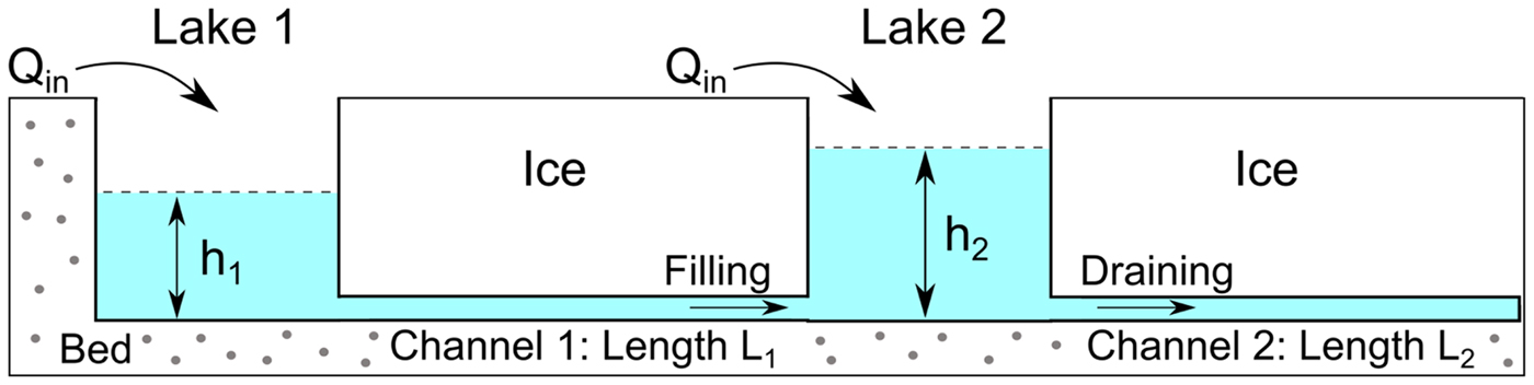
We assume that a sequence of ice-dammed lakes are hydraulically connected by subglacial channels (Fig. 1). The mathematical model consists of two components. The first component is a set of PDEs that governs the evolution of the subglacial channels. The second component is a simple evolution equation for the lakes. Following Fowler (Reference Fowler1999, Reference Fowler2009), the lake evolution equations provide the boundary conditions for the subglacial channels where they are connected to the lakes. While we only explore two connected lakes here, we formulate the model for an arbitrary number of lakes.
Schematic diagram of connected lake model setup. Upstream and downstream lake depths are noted by h 1 and h 2, respectively. The upstream and downstream channel lengths are noted by L 1 and L 2. The meltwater supply rate to the lakes is Q in. Arrows in the subglacial channels note the water flow direction.
2.1 Subglacial channel model
We let S be the cross-sectional area of the semi-circular subglacial channel, Q the water discharge, Ψ the hydraulic gradient, x the distance along the channel and t time. We define the effective pressure N to be the difference between the ice overburden pressure and the water pressure in the channel. We assume that the water in the channel and the ice at the channel walls are always at the melting point and we neglect heat advection (Nye, Reference Nye1976). We further assume that the ice creeps as a shear-thinning viscous fluid (Nye, Reference Nye1953; Glen, Reference Glen1955; Cuffey and Paterson, Reference Cuffey and Paterson2010).
The magnitude of water discharge through the subglacial channel is partially determined by the hydraulic gradient

which includes the effective pressure gradient and a background hydraulic gradient, ψ. We choose the parameterization

where L c is the length of the subglacial channel and ψ0 is the hydraulic gradient scale. This parameterization is based on a fit to surface and bed slopes at Grímsvötn (Fowler, Reference Fowler2009). We use this parameterization because it allows water flow toward the lake between floods, which has previously been found to promote long-term stability of filling–draining oscillations (Fowler, Reference Fowler2009; Kingslake, Reference Kingslake2015). Within ~ L c/20 km of the lake, the hydraulic gradient Ψ is strongly influenced by ψ. We expect that other parameterizations would also allow for stable filling–draining cycles based on the success of the spatially-uniform model in ‘Simplified model’ section.
Conservation of ice mass is satisfied through a balance of melting and viscous closure rates at the channel walls. The channel size evolves according to

where ρi is the ice density, l is the latent heat of melting, and $\hat {A}$ and n are the parameters in Glen's flow law (Glen, Reference Glen1955; Cuffey and Paterson, Reference Cuffey and Paterson2010). In Eqn (3), the melt and closure rates are proportional to QΨ and SN|N|n−1, respectively.
Conservation of mass for water in the channel requires
where ρw is the water density and μ is a constant source term for water that enters the channel through drainage pathways such as cavities and moulins (Fowler, Reference Fowler1999, Reference Fowler2009; Kingslake, Reference Kingslake2015). We note that μ has a stabilizing effect because it prevents the channel from closing completely. Combining Eqn (4) with Eqn (3), we obtain

Finally, the Darcy–Weisbach law for turbulent water flow through pipes provides a relation between channel size, pressure and discharge through the equation

where f d is the friction factor (Clarke, Reference Clarke2003). We list the numerical values of the above parameters in Table 1.
Model parameters and physical constants used in simulations. These values are fixed unless noted otherwise.

A − in the fourth column denotes a dimensionless quantity.
2.2 Lake model
We suppose that the first upstream lake (Lake 1 in Fig. 1) is connected only to a downstream channel. We let h be the lake depth, H the ice thickness and A the lake surface area. We hold the ice thickness and lake surface area constant. Alternatively, if the geometry of the lake is known then one may prescribe the surface area as a function of the lake depth. We let Q in be the volumetric rate of meltwater flow into the lake from runoff, englacial storage and other sources. Below, we denote the water discharged from the lake through the downstream channel by $Q_{\rm out}^{\rm ch}$ . The lake depth evolves according to

Assuming hydrostatic balance, the effective pressure at the lake is

This relation between lake depth and effective pressure in Eqn (8) leads to the evolution equation

For downstream lakes (e.g., Lake 2 in Fig. 1), there is an additional input $Q_{\rm in}^{\rm ch}$ from the upstream channel. In this case, the effective pressure at the lake evolves as

2.3 Boundary conditions
The lake evolution Eqn (10) determines the boundary conditions for the channel equations everywhere except at the terminus. At the terminus, we impose the boundary condition N = 0. As discussed by Evatt (Reference Evatt2015), the zero pressure condition at the terminus leads to the problem of a forever-widening channel there. Although observations suggest that subglacial channels widen at the terminus (Drews and others, Reference Drews2017), unbounded growth is unreasonable. Therefore, we scale the viscous closure law by

which arises from the assumption of finite ice depth (Evatt, Reference Evatt2015). The viscous closure rate in Eqn (3) becomes SN|N|n−1ζ(S). For large S f, ζ(S) ≈ 1 away from the terminus. Most importantly, S can never exceed S f (Evatt, Reference Evatt2015). We have found that using S f = 8000 m2 in numerical experiments does not alter the solutions near the lake qualitatively and prevents the channel from growing without bound.
2.4 Scaling
Here we introduce a scaling for the subglacial channel Eqns (1–6). We introduce the dimensionless variables

and choose the scales

where A 1 is the surface area of the first (upstream) lake. The scale $\tilde {S}$ is the channel size at the equilibrium discharge Q = Q in in the absence of effective pressure gradients. The scale $\tilde {t}$
 is the intrinsic filling timescale of the first upstream lake. Likewise, the melting timescale for the channel at the equilibrium discharge is

The quantity

is the viscous closure timescale for the channel, which depends strongly on the channel length. We define the dimensionless parameters

which are the melting and closure timescales normalized by the filling timescale. The parameters a m and a c control the magnitudes of the melting and closure rates, respectively.
2.5 Generalized connected lake system
Here we complete the formulation of the model by generalizing Eqns (1)–(6) and the boundary condition Eqn (10). We consider a system with M lakes and channels on a glacier of length L c. We let L k be the length of the k-th subglacial channel, subject to

The scaled length of each subglacial channel is

so that the total length of the scaled system is one. Supposing that the system (1)–(6) holds on each interval (0, L k*), the scaling described by Eqns (12–16) leads to the system of partial differential equations


for $k=1\ldots M$ . Above, $\mu_{\ast} = \mu \tilde {x}/\tilde {Q}$
 , $b_{\rm m} = (({\rho_{\rm w}-\rho_{\rm i}})/{\rho_{\rm w} \rho _{\rm i} l}) \tilde {N}$
 , and $b_{\rm c} = 2\hat {A}n^{-n} \tilde {x} \tilde {S} \tilde {N}^n / \tilde {Q}$
 . The parameters b m and b c are small and the associated terms may be neglected, although we do not do so here. We let A k be the surface area of each lake. To satisfy the lake evolution Eqn (10), we enforce the non-dimensionalized upstream boundary conditions

for k > 1, where we have defined A k* = A k/A 1. We refer to A k* as the relative size of the k-th lake. For the first lake, the non-dimensional boundary condition is

Likewise, the downstream boundary conditions are

for k < M, with the modification at the terminus

Above we have assumed that the effective pressure is uniform across each lake. Moreover, we assume that $L_k^{\ast}\; \gtrsim\; 1/20$ so that the parameterization ψ*(x *) does not dominate the hydraulic gradient Ψk. Equations (19)–(26) constitute a complete mathematical model for connected glacial lakes. When discussing single-lake systems, we will omit the k subscripts on the variables. The system is solved numerically using a finite element method. We provide details on the numerical method and implementation in Appendix A.
3. Results
3.1 Single-lake model
We first study the behavior of a single-lake system (M=1) to develop physical intuition into the oscillatory nature of the model before considering the multiple-lake model. We assume that Q in is constant in time for all experiments. In the figures and discussion below we denote the discharge out of the lake by Q L = Q(0, t). For clarity, we plot the lake depth h(t) rather than the effective pressure at the lake N(0, t). These quantities are related through Eqn (8). The single-lake results outlined below may be compared to previous modeling studies (Fowler, Reference Fowler1999, Reference Fowler2009; Kingslake and Ng, Reference Kingslake and Ng2013a; Kingslake, Reference Kingslake2015).
The fundamental feature of the model is that the boundary condition in Eqn (24) forces oscillations in lake depth, effective pressure, discharge and channel size (Figs 2a, b). The physical mechanism for single-lake oscillation originates from the coupling of the melting and closure rates to discharge and channel size. The lake depth h increases slowly until the channel melts open enough for rapid drainage to begin (point h max in Fig. 2b). The discharge Q L grows during the flood, causing the channel to open rapidly due to melting. The positive feedback between discharge and channel size causes a sharp increase in melt rate. At the same time, increasing discharge causes the lake level to decrease rapidly. This melt-opening feedback persists to the peak of the flood (point Q max in Fig. 2b). Eventually the channel begins to collapse once it becomes too large. Water flow through the channel becomes increasingly constricted as the channel closes, diminishing the melt rate and ending the flood. The lake then begins to refill because the channel is small again (Fig. 2b).
Numerical simulations of a single-lake system for Q in = 5 (a and b) and 15 m3s−1 (c and d). The solutions are plotted over time (a and c) and in Q L − h phase space (b and d). Arrows in panels (b) and (d) show the direction of the trajectories in phase space. Maximum lake depth and discharge are noted by the points labeled h max and Q max, respectively. The lake surface area is A = 1 km2. Note that when Q in = 15 m3s−1 (panels c and d), the discharge approaches the equilibrium value Q L = Q in. The dimensionless parameters are (a m, a c) = (66, 2900) (a and b) and (a m, a c) = (28, 967) (c and d).
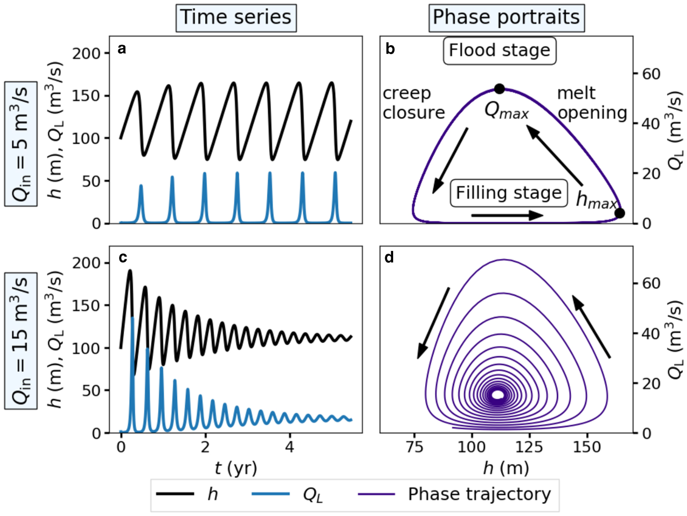
The oscillations in h and Q L approach periodic functions over time for a range of meltwater input (Q in) values (Fig. 2a). These periodic functions define a limit cycle – a closed curve in Q L-h phase space (Fig. 2b). All solutions that start away from equilibrium will approach the limit cycle except at higher values of Q in. The behavior at high Q in is explored in the next paragraph and in greater detail in ‘Simplified model’ section. The oscillation frequency is controlled primarily by the meltwater input Q in and the lake size A because the natural filling timescale for the lake $\tilde {t}$ is proportional to A/Q in in Eqn (13). Large lakes oscillate slowly because they take longer to fill at a fixed Q in. Conversely, a higher meltwater supply results in more frequent cycles.
Once Q in increases past some critical threshold, the oscillations damp toward equilibrium where the lake drains water continuously at a constant rate (Fig. 2c). In phase space, the damping appears as a spiral (Fig. 2d). Damping occurs because the filling timescale $\tilde {t}$ in Eqn (13) becomes too small relative to the melting timescale t m in Eqn (14) and viscous closure timescale t c in Eqn (15) for oscillations to be sustainable. Likewise, the melting strength a m and closure strength a c parameters in Eqn (16) become small and perturbations to the equilibrium solution are not able to grow. In this scenario, the discharge out of the lake approaches the equilibrium value Q L = Q in (Figs 2c, d). We explore the transition from oscillation to damping further in ‘Simplified model’ section with a reduced ODE model.
3.2 Double-lake models
Connected lakes can oscillate in a variety of different ways that are distinct from the single-lake solutions discussed in the previous section. However, these double-lake oscillations follow the same physics of the single-lake system. We explore the amplitudes and frequencies of these oscillations as the downstream lake surface area, and the spacing between the lakes is varied since these are easy parameters to estimate in natural systems. We choose the values of A 1 = 1 km2 and Q in = 5 m3s−1 in order to determine appropriate values for a m and a c. However, these results apply to systems with other lake sizes and meltwater supply rates if the ratio A/Q in is similar to what we have chosen. Unless stated otherwise, we use (a m, a c) = (66, 2900). This parameter choice corresponds to the single-lake solution with undamped oscillations (Figs 2a, b). The scaling shows that the trends outlined below are due to the relative downstream lake size A 2* = A 2/A 1 and the magnitude of the meltwater supply rate relative to the lake sizes. The behavior of the upstream lake always resembles the single-lake solutions due to the constant meltwater input. The downstream lake behavior is modified by the additional time-dependent water input from the upstream channel, Q 1(L 1*, t), and the parameter variations discussed below.
Lake spacing examples
First, we explore the influence of lake spacing on the depth-discharge oscillations. The length of the whole domain is always preserved since we set L 2* = 1 − L 1* and vary L 1*. In this series of examples, we keep the size of the second lake constant and equal to the first lake (A 2* = 1). In general, we find that the lakes oscillate in phase when they are closely spaced ($L_1^{\ast} \lesssim 0.5$ ). When the lakes are far apart ($L_1^{\ast}\; \gtrsim\; 0.5$
 ), we observe small-amplitude oscillations in the downstream lake that are delayed relative to the upstream cycles.
When lakes are closely spaced, both lakes damp toward equilibrium (Fig. 3a). For our parameter choices this occurs when L 1* < 0.5, but sets in strongly around L 1* = 0.1. Damping occurs in shorter channels because the closure rate becomes small relative to the melt rate, similar to the transition to damping with increasing meltwater supply rate. In single-lake systems, the closure rate decreases strongly as the channel length decreases because the closure magnitude parameter a c is proportional to $L_{{\rm c}}^{n+1}$ in Eqn (16). The system approaches equilibrium because the channel cannot close quickly enough to sustain oscillations. The same effect occurs in the double-lake system, although the change is in the length of the subdomains rather than the parameter a c. Interestingly, the single-lake solution exhibits undamped oscillations for the same choice of parameters (a m, a c).
Simulations of equally-sized lakes (A 2* = 1) as the scaled upstream channel length L 1* changes. We choose (a) L 1* = 0.1, (b) L 1* = 0.5 and (c) L 1* = 0.75.

When the lakes are far apart ($L_1^{\ast}\; \gtrsim\; 0.6$ ), draining of the downstream lake is consistently delayed and the oscillations have smaller amplitudes than the upstream lake (Fig. 3c). Delayed oscillations in distant lakes occur because pressure variations caused by draining of the upstream lake take longer to reach the downstream lake. In each cycle, the downstream lake depth reaches the flotation level h = (ρ i/ρ w)H and then drains rapidly. The reduced amplitude of the downstream lake oscillations is a consequence of the downstream lake draining through a shorter channel. The downstream lake continuously drains water between floods because the closure rate is small in the downstream channel, leading to a large inter-flood channel size. The downstream lake oscillations are forced by the upstream floods, in contrast to the self-sustained oscillations in the upstream lake.
If the lakes are evenly spaced (L 1* ≈ 0.5), they oscillate with similar amplitudes (Fig. 3b). A common feature in this scenario is the presence of multiple peaks per cycle in the downstream depth and discharge timeseries. When the lakes are the same size, as in this example, the downstream lake may have alternating double and single peaks (Fig. 3b). Multiple-peaked cycles are explored further in the following section.
Smaller downstream lake
Now we fix L 1* = 0.5 and study the effect of decreasing the relative downstream lake size A 2*. The frequency of downstream lake oscillations increases with decreasing lake size (Fig. 4). In the limit of a very small surface area (A 2* ≈ 0.01), the downstream lake behaves as a manometer that records the mean effective pressure in the channel (Fig. 4f)(Anderson and others, Reference Anderson, Walder, Anderson, Trabant and Fountain2005; Carter and others, Reference Carter, Fricker and Siegfried2013). The downstream lake depth is essentially constant except for when the upstream lake begins to drain. The downstream lake then fills rapidly and drains in phase with the upstream lake. Multiple peaks in downstream lake depth per upstream cycle occur when A 2* is larger than ~0.01 (Figs 4a–e). When multiple peaks exist in the downstream lake depth timeseries, the final peak coincides with draining of the upstream lake. The overall period of the downstream lake's filling–draining cycle conforms to that of the first lake due to the periodic arrival of the additional water input Q 1(L 1*, t). The upstream floods force the downstream lake to oscillate at the same overall frequency.
Simulations with smaller downstream lake size. The scaled upstream channel length is L 1* = 0.5. The relative downstream lake sizes are (a) A 2* = 0.49, (b) 0.36, (c) 0.25, (d) 0.16, (e) 0.09 and (f) 0.01.

If the lakes were not coupled, the downstream lake would resemble the upstream one except with higher frequency. The closest example to uncoupled behavior occurs around A 2* = 0.49 where the second lake has two large, well-formed peaks (Fig. 4a). The transition from large to small intervening oscillations occurs around A 2* ≈ 0.36 (Fig. 4b). The small intervening oscillations are not associated with significant discharge out of the downstream lake. The amplitudes of the intervening oscillations decrease continuously as lake size decreases (Figs 4b–f).
Larger downstream lake
When the relative downstream lake size A 2* is increased above unity, the lakes cease to oscillate in phase (Fig. 5). There is a small size range (A 2* ≈ 2.25) where the lakes demonstrate antiphase oscillations (Fig. 5a). If the lakes were uncoupled, the downstream lake would oscillate at a lower frequency due to its large size. The additional input Q 1(L 1*, t) allows the downstream lake to oscillate at the same frequency if it is not too large. More precisely, the downstream lake will oscillate at a frequency similar to the upstream lake's frequency if $A_2/(Q_{\rm in} + \bar {Q}_1)$ is similar to A 1/Q in, where $\bar {Q}_1$
 is the mean of Q 1(L 1*, t) over one upstream cycle. Because the additional water input from the upstream flood must be received during the downstream filling stage, the lakes must oscillate out of phase. The effect of the additional water input is reflected in the timeseries (Fig. 5a). Between floods, the downstream lake level increases slowly at first, ramps up during the upstream flood, then fills slowly again before draining. The slow-filling stage represents the natural, uncoupled filling rate of the downstream lake.
Simulations of larger downstream lakes. The scaled upstream channel length is L 1* = 0.5 for both examples. The relative downstream lake sizes are (a) A 2* = 2.25 and (b) 16.
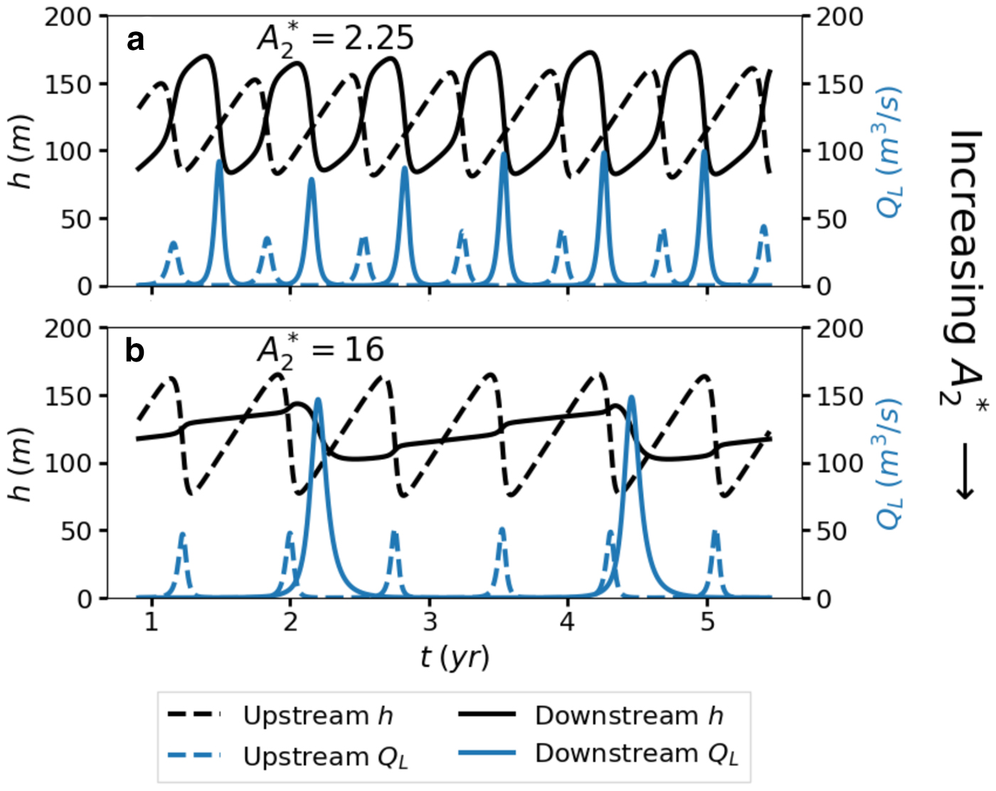
If the downstream lake is much larger than the upstream lake, it essentially acts as a storage tank (Fig. 5b). The lake level increases steadily at its natural rate until each upstream flood when a sharp uptick occurs. The sharp upticks superimposed on the natural filling rate lead to a staircase-like appearance in the downstream depth timeseries (Fig. 5b). After several upstream cycles, the downstream lake finally drains, releasing large volumes of water.
Meltwater variations
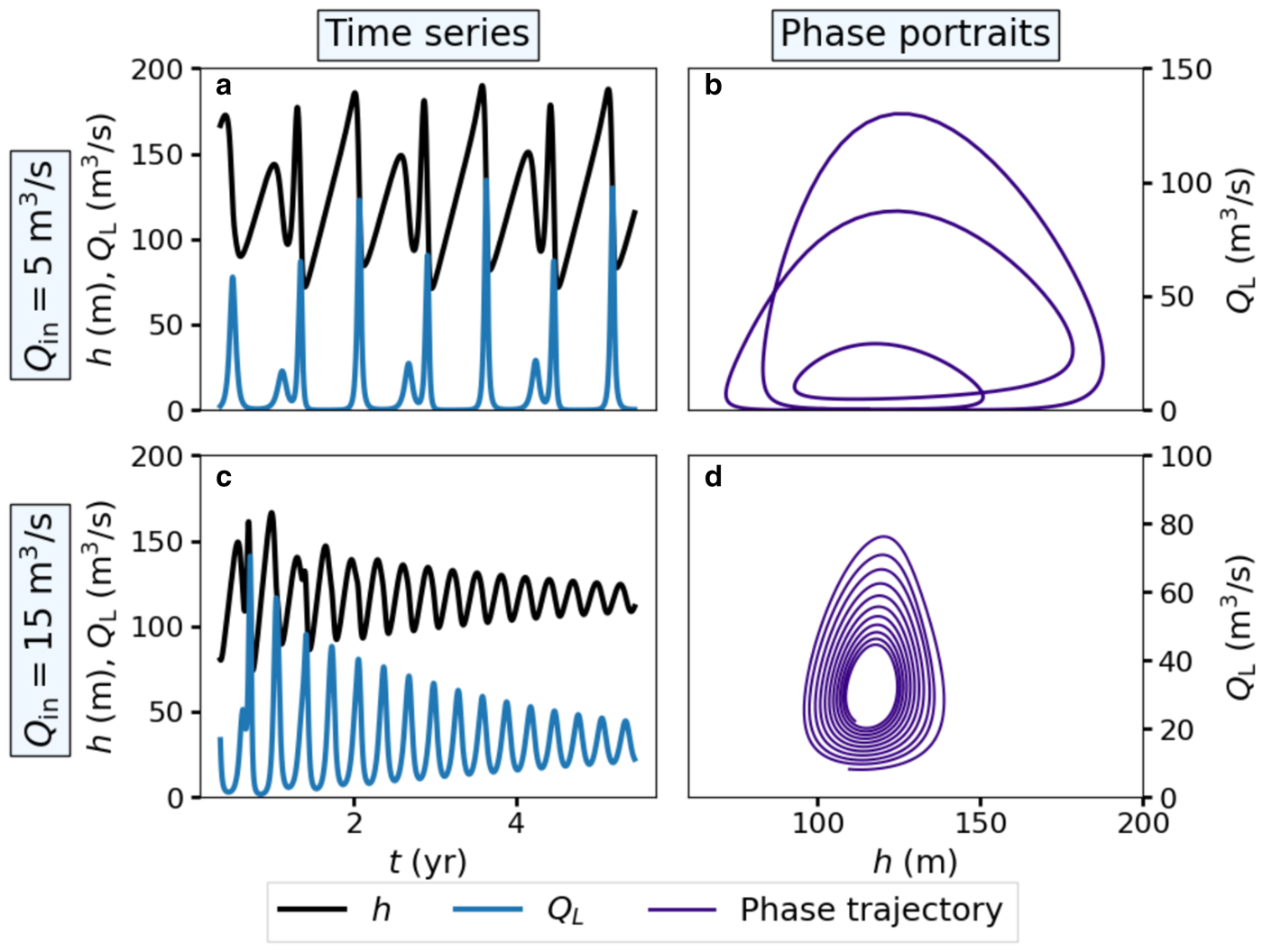
In contrast to the geometrically simple limit cycles in the single-lake system (Fig. 2b), the downstream lake oscillations (e.g., Fig. 6a) can exhibit complex patterns in phase space (Fig. 6b). As with the single-lake system, damping due to an increase in meltwater supply also occurs in the double-lake system (Figs 6c, d). In this scenario, both lakes approach equilibrium simultaneously. The physical mechanism for damping is the same as in the single-lake system. At high Q in, the filling timescale $\tilde {t}$ is too fast relative to the melting t m and closure t c timescales to support oscillations. The transition from oscillation to stable equilibrium is a fundamental feature of the model. We explore this bifurcation further in the following section.
Numerical simulations of a double-lake system for Q in = 5 (a and b) and 15 m3s−1 (c and d). The relative downstream lake size is A 2* = 1 and the scaled upstream channel length is L 1* = 0.5. The solutions for the downstream lake are plotted over time (a and c) and in Q L-h phase space (b and d). The solutions for the upstream lake are not plotted because they are nearly identical to those in Fig. 2. Note that when Q in = 15 m3s−1 (panels c and d), the discharge approaches the equilibrium value Q L = 2Q in. The dimensionless parameters are (a m, a c) = (66, 2900) (a and b) and (a m, a c) = (28, 967) (c and d).
4. Simplified model
Here we explore an ODE model for the connected lake system in order to gain insight about lake behavior as the meltwater supply rate varies. Additionally, solving the ODE model numerically is significantly more computationally efficient than solving the PDE model. We assume that S, N and Q are spatially uniform near each lake. Then, the channel evolution in Eqn (19) and upstream boundary condition (23) form the dynamical system


In order to simplify the analysis, we have neglected the closure rate scale ζ(S) in Eqn (11). Including this leads to better quantitative agreement with the PDE model, but does not change the qualitative structure of the bifurcations. The first lake's upstream boundary condition in Eqn (23) becomes

We introduce a regularized Darcy–Weisbach law

where $\varepsilon_{\ast} = \varepsilon /\tilde {S}$ , for some small parameter ε. Equation (30) ensures that the channel size is bounded below by some positive value. Regularization is necessary to produce the limit cycles and bifurcations that exist in the PDE model. An unregularized version of the simplified model presented here with ε = 0 and constant Ψ was studied previously by Fowler (Reference Fowler1999) and Ng and Björnsson (Reference Ng and Björnsson2003). Local stability analysis and numerical experiments were used to suggest that limit cycles do not exist in the unregularized model (Fowler, Reference Fowler1999; Ng and Björnsson, Reference Ng and Björnsson2003). Using an energy argument, we extend this result by showing that all non-equilibrium solutions to the unregularized model are globally unstable and blow up if α > 1 (Appendix B). However, for α = 1 all non-equilibrium solutions are periodic orbits that resemble the limit cycles in the single-lake system. In the case of α = 1, the level curves of the energy function provide an approximate algebraic relation between S and N during single-lake flood cycles (Appendix B).
The governing equations may be stabilized in several other ways. For example, an equivalent regularization is to modify the closure term to (S − $\varepsilon_*$ )N|N|n−1 so that the channel ceases to close at some small size, while keeping the usual Darcy–Weisbach law. The solutions associated with this regularization will only differ from ours by the small additive constant $\varepsilon_*$
 . A third possible regularization is to add a small parameter to Eqn (27), which may be interpreted as an opening rate due to basal sliding (Schoof, Reference Schoof2010). These ‘regularizations’ have the same stabilizing effect as the channel source term μ in the PDE model Eqn (4) because they prevent the channel from closing completely.
To complete the simplified model, we introduce a forward difference approximation of the dimensional hydraulic gradient $\Psi _k^{\rm d} = {\psi }_0 - N_k/L_{k}$ . We neglect downstream pressure contributions to the upstream hydraulic gradient under the assumption that upstream pressure variations are dominated by upstream lake activity. With this parameterization, the upstream lake is completely decoupled from the downstream lake. This may be inappropriate for closely spaced lakes because the downstream lake may strongly influence the upstream channel. This approximation corresponds to the scaled hydraulic gradient

The simplified model described by Eqns (27–31) produces results that are qualitatively consistent with those from the PDE model. All oscillatory behaviors discussed for the double-lake system exist in the simplified model for similar parameter choices (Fig. 7). Moreover, the oscillations damp as Q in increases past some critical threshold, as in the PDE model (Appendix C). We provide a quantitative comparison of the ODE and PDE models in Appendix D. The advantage of Eqns (27–31) is that they may be studied using dynamical systems theory (Chicone, Reference Chicone2006; Kuznetsov, Reference Kuznetsov2004; Strogatz, Reference Strogatz2018).
Numerical results from the simplified model in Eqns (27 and 28) for double-lake systems compared with the PDE results from 'Results' section. For the ODE results we choose the hydraulic gradient scale ψ0 = 75 Pa m−1, ε = 0.1 m2 and glacier length L c = 40 km. The scaled upstream channel length is L 1* = 0.5 except in panels (g) and (h). The parameters we choose are (a) A 2* = 0.01, (b) A 2* = 0.01, (c) A 2* = 0.16, (d) A 2* = 0.16, (e) A 2* = 0.81, (f) A 2* = 1, (g) A 2* = 0.81 and L 1* = 0.75, (h) A 2* = 1.0 and L 1* = 0.75, (i) A 2* = 2.25, (j) A 2* = 2.25, (k) A 2* = 16 and (l) A 2* = 16.

4.1 Bautin bifurcation
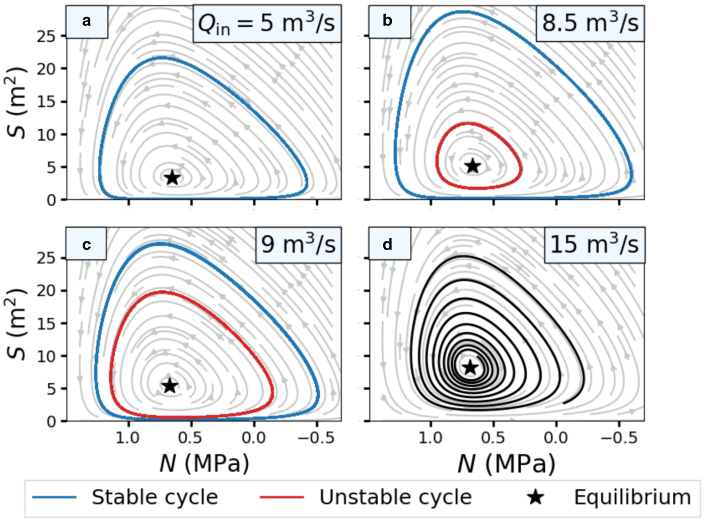
Single-lake and multiple-lake systems damp toward equilibrium once a critical value of the meltwater source parameter is reached (Figs 2c, d and 6c, d). Based on the numerical experiments, Fowler (Reference Fowler1999) suggested that this transition occurs due to a Hopf bifurcation. Numerical results show that the transition occurs because Eqns (27) and (28) undergo a Bautin (generalized Hopf) bifurcation as Q in varies (Figs 8 and 9). The Bautin bifurcation is a combination of a supercritical Hopf bifurcation, subcritical Hopf bifurcation and saddle-node bifurcation of cycles (Kuznetsov, Reference Kuznetsov2004).
Phase portraits of the simplified model in Eqns (27 and 29) for a single-lake system with varying meltwater supply. The meltwater supply rates for each panel are (a) Q in = 5, (b) 8.5, (c) 9 and (d) 15 m3s−1. Limit cycles are plotted for t > 315 years. We choose the parameters A = 1 km2, ε = 0.05 m2, ψ0 = 45 Pa m−1 and L c = 40 km. The dimensionless parameters are (a) (a m, a c) = (10, 108), (b) (a m, a c) = (6.2, 63.4), (c) (a m, a c) = (5.9, 59.8) and (d) (a m, a c) = (4, 36).
Bifurcation diagram for the ODE model of a single-lake system in Eqns (27 and 29) for various values of ε. The bifurcation parameter is Q in. Limit cycle amplitudes are defined as max (S(t)) for t > 315 years. Unstable limit cycle amplitudes are computed by solving the time-reversed system of equations. We choose A = 1 km2, ψ0 = 45 Pa m−1 and L c = 40 km. Labeled points correspond to the (i) supercritical Hopf bifurcation, (ii) subcritical Hopf bifurcation and (iii) saddle-node bifurcation of cycles.
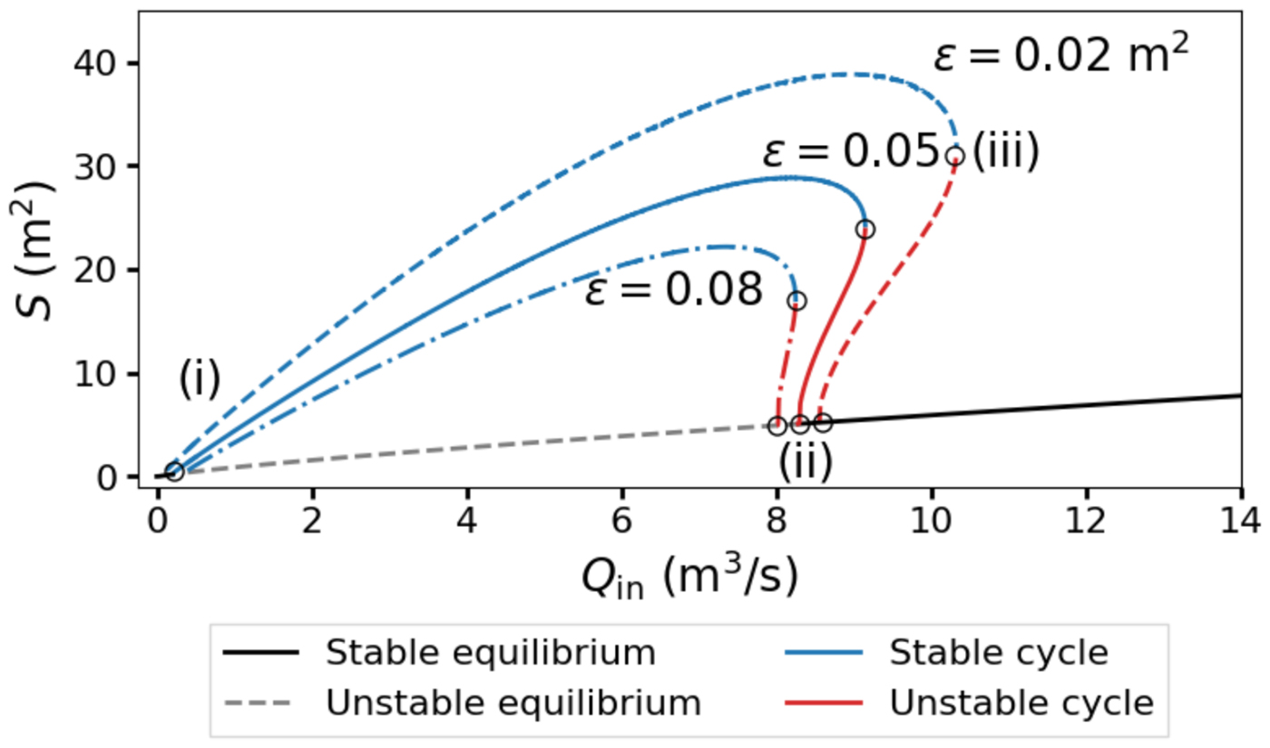
The individual bifurcations occur sequentially as Q in increases. The supercritical Hopf bifurcation is characterized by the appearance of a stable limit cycle at some small Q in ≪ 1 (Fig. 9 point i). As Q in increases, the amplitude of the stable cycle grows (Fig. 8a) until the subcritical bifurcation occurs. At the subcritical Hopf bifurcation, an unstable limit cycle appears inside of the stable cycle (Figs 8b and 9 point ii) and grows rapidly (Fig. 8c). The unstable limit cycle soon annihilates the stable cycle in a saddle-node bifurcation of cycles, leaving behind only a stable spiral node (Figs 8d and 9 point iii). The values of Q in where these bifurcations occur are noted in Figure 9, but depend on ε and the other parameters that determine a m and a c in Eqn (16).
The stability transitions are related to the sign of tr(J), the trace of the Jacobian of Eqns (27) and (28) evaluated at the equilibrium. The trace may be written as

where S e is the equilibrium channel size (Appendix C). For fixed ε, we have that $\varepsilon_{\ast} \propto Q_{\rm in}^{-\textstyle{{1}/{\alpha}}} \to \infty$ as Q in → 0. Equation (32) then implies that tr(J) < 0 for sufficiently small Q in, meaning that the equilibrium becomes stable. This stability transition is a necessary condition for the supercritical Hopf bifurcation (Fig. 9 point i).
At the subcritical Hopf bifurcation (Figs 8b and 9 point ii), the equilibrium becomes stable because the meltwater supply increases past some critical value, as observed in the numerical results. The sign of tr(J) is equal to the sign of the function

where N e is the equilibrium effective pressure. For a constant ratio a c/a m and fixed ε*, N e and the quantity in square brackets in Eqn (29) are also fixed (Appendix C). Thus, varying a c or a m at a fixed ratio changes the sign of ${\cal T}$ , resulting in stability transitions. In particular, increasing Q in leads to decreasing a m and, eventually, ${\cal T} \lt 0$
 . This condition implies that the equilibrium is locally stable, and, therefore, explains the damping with increasing meltwater supply. Likewise, ${\cal T} \gt 0$
 implies that the equilibrium is locally unstable. We plot the sign of ${\cal T}$
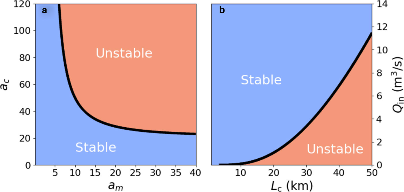
 in the a m-a c plane in Figure 10a and in the L c-Q in plane in Figure 10b. Physically, the equilibrium becomes stable because the filling timescale $\tilde {t}$
 in Eqn (13) becomes small relative to the melting t m and closure t c timescales. Since the channel evolves too slowly relative to the meltwater supply rate, perturbations to steady state return to equilibrium. These stability transitions generalize to systems with arbitrary numbers of lakes (Appendix C).
Sign of tr(J) evaluated at equilibrium for a range of a m and a c for the single-lake ODE model. The positive region (red) corresponds to an unstable equilibrium and the negative region (blue) corresponds to a stable equilibrium. We hold ε* = 0.05 constant. For panel (b), we choose the parameters ψ0 = 45 Pa m−1 and A = 1 km2 to compute ${\cal T}(a_{\rm m}(Q_{\rm in},\,L_{\rm c}),\,a_{\rm c}(Q_{\rm in},\,L_{\rm c}))$ in Eqn (33), where the equilibrium pressure N e depends on a m and a c through solution of the non-linear Eqn (C5). Note that this stability diagram is for fixed ε* so that the stability transition at small Q in with fixed ε (Fig. 9 point i) is not observed.
For a range of Q in near the subcritical Hopf bifurcation, there exists an unstable limit cycle around the stable fixed point (Figs 8b, c). In this region of parameter space, the asymptotic behavior of the solution depends on the initial condition. In particular, channels that are far from equilibrium approach the stable limit cycle. Intuitively, this difference in asymptotic behavior occurs because trajectories starting far from equilibrium pass through larger values of S and Q that admit higher melting and closure rates. Sustained oscillations are then possible since the channel evolution keeps pace with the filling rate. However, the melting strength a m and closure strength a c parameters are small enough to also admit solutions that converge to equilibrium. The equilibrium and stable limit cycle are very weak attractors in this parameter range. Convergence to the limit set can take more than one hundred years.
5. Discussion
Several natural lake systems exhibit behavior that is qualitatively similar to our numerical results. The Hidden Creek–Donoho Falls lake system in Alaska provides an example of a smaller downstream lake that is in phase with the upstream filling–draining cycle (Bartholomaus and others, Reference Bartholomaus, Anderson and Anderson2008, Reference Bartholomaus, Anderson and Anderson2011). Hidden Creek lake drains on a yearly cycle and the downstream lake (Donoho Falls) drains in phase with this, but also oscillates intermittently. Numerical results in Figures 4b–f show similar behaviors where the downstream lake has several small-amplitude oscillations between the main draining events that are in phase with the upstream lake. In this case, smaller downstream lakes may act as pressure gauges that are sensitive to upstream lake cycles (Anderson and others, Reference Anderson, Walder, Anderson, Trabant and Fountain2005). Observations suggest that ‘through-flowing’ subglacial lakes may behave in a similar manner (Carter and others, Reference Carter, Fricker and Siegfried2013; Siegfried and Fricker, Reference Siegfried and Fricker2018).
The multiple-peaked downstream cycles explored here (Fig. 4) are similar in nature to the water pressure doublets studied by Schoof and others (Reference Schoof, Rada, Wilson, Flowers and Haseloff2014), despite the difference in timescales and water storage mechanisms. The pressure doublets result from a distributed storage model forced with time-varying water input (Schoof and others, Reference Schoof, Rada, Wilson, Flowers and Haseloff2014). The similarity to the multiple-peaked lake cycles likely arises because the downstream lake in our model is forced by time-varying water input from the upstream channel. If the storage capacity is small relative to the filling rate, higher oscillation frequencies should be expected in both models.
Observations of lake systems in Antarctica also support our model. Delayed filling–draining events have been observed in East Antarctica (Wingham and others, Reference Wingham, Siegert, Shepherd and Muir2006), the lower MacAyeal Ice Stream, and Slessor Glacier (Siegfried and Fricker, Reference Siegfried and Fricker2018). The out-of-phase oscillations depicted in Figure 5 are most similar to these observations. Out-of-phase oscillation requires the downstream lake to be larger than the upstream lake in the model. In the case of the MacAyeal Ice Stream, the downstream lake Mac1 is indeed slightly larger than the upstream lake Mac3 (Siegfried and Fricker, Reference Siegfried and Fricker2018). Similarly, filling of the larger lake on Slessor Glacier (Slessor3) during 2005–2015 was coincident with the draining of the smaller adjacent lake (Slessor2) (Siegfried and Fricker, Reference Siegfried and Fricker2018). However, in the case that these are in fact a single lake (Slessor23), as suggested by Siegfried and Fricker (Reference Siegfried and Fricker2018), this analysis is not applicable. An improved theory of how connected subglacial lakes behave could help clarify whether or not these are distinct lakes.
For similar-sized lakes, we have shown that double-peaked drainage events are possible in the downstream lake. Double-peaked events have been observed in a lake system at the confluence of the Whillans and Mercer ice streams in West Antarctica (Fricker and Scambos, Reference Fricker and Scambos2009; Siegfried and others, Reference Siegfried, Fricker, Carter and Tulaczyk2016; Siegfried and Fricker, Reference Siegfried and Fricker2018). Between 2004 and 2008, two downstream lakes, Mercer Subglacial Lake (SLM) and L7, exhibited double-peaked filling–draining events that were roughly in phase with the upstream Subglacial Lake Conway (SLC). Following the first peaks in the downstream lakes, SLC drained and the downstream lakes drained again soon after. The filling–draining cycle in the Whillans–Mercer system repeated between 2010 and 2015 (Siegfried and others, Reference Siegfried, Fricker, Carter and Tulaczyk2016; Siegfried and Fricker, Reference Siegfried and Fricker2018). During this cycle, both SLM and L7 displayed double peaks again, although SLM's second peak was much smaller than in the first cycle. The SLM cycle is qualitatively similar to the alternating single–double peak cycles in Figures 6 and 7.
The alternative to oscillation is steady lake drainage. Our ODE model results suggest that oscillations may not be possible in cases where the lake filling rate is either much slower or faster than the channel evolution timescales (Fig. 9). An example of this behavior may occur at Lake Vostok, which has been inactive for at least a decade (Richter and others, Reference Richter2014). However, Evatt and others (Reference Evatt, Fowler, Clark and Hulton2006) simulated filling–draining cycles in Vostok-sized lakes with a model similar to the one used here. The oscillation period of Vostok was estimated to be at least 5000 years (Evatt and others, Reference Evatt, Fowler, Clark and Hulton2006). It is possible that Lake Vostok is so large that its filling rate would be too low for us to detect during quiescent, inter-flood periods.
While we see similarities between our numerical results and data from Antarctica, a complete model for subglacial lake drainage would include ice deformation over the lake. Inclusion of this would lead to a different functional relationship between the effective pressure and the lake depth, or different boundary conditions at the lakes (Evatt and others, Reference Evatt, Fowler, Clark and Hulton2006; Evatt and Fowler, Reference Evatt and Fowler2007). This should result in oscillations that are closer in magnitude to observations of Antarctic subglacial lake activity. Ice flow also influences the evolution of the hydraulic gradient around the lake because filling and draining events lead to changes in surface slopes. Likewise, changes in ice thickness may also influence subglacial lake drainage events. We leave exploration of such models for future work but expect that the basic trends outlined here will hold.
Subglacial flooding in Antarctica has led to enhanced ice flow on several glaciers (Stearns and others, Reference Stearns, Smith and Hamilton2008; Scambos and others, Reference Scambos, Berthier and Shuman2011; Fricker and others, Reference Fricker, Siegfried, Carter and Scambos2016; Siegfried and others, Reference Siegfried, Fricker, Carter and Tulaczyk2016). Ice deformation is usually related to effective pressure at the base through a sliding law. Understanding basal sliding in a drainage system during floods requires determining the evolution of effective pressure in all of the drainage elements. Realistic drainage basins include interacting channels, cavities, water sheets, canals, moulins and other drainage pathways (Creyts and Schoof, Reference Creyts and Schoof2009; Schoof, Reference Schoof2010; Hewitt, Reference Hewitt2011; Werder and others, Reference Werder, Hewitt, Schoof and Flowers2013). Our single-lake results are similar to those obtained by Kingslake and Ng (Reference Kingslake and Ng2013a) who included a one-dimensional cavity model. Even so, it is unclear how a two-dimensional network of drainage elements would respond to oscillatory lake drainage. In the same vein, alternative hydrology models like the canal model of Walder and Fowler (Reference Walder and Fowler1994) may lead to better quantitative agreement with observations of Antarctic filling–draining events (Carter and others, Reference Carter, Fricker and Siegfried2017).
An important question is whether infrequent large floods or frequent small floods lead to longer periods and higher magnitudes of enhanced sliding. Large lakes may temporarily shield the downstream drainage system from frequent upstream floods (Fig. 5). Counterintuitively, a larger upstream lake may also protect the downstream glacier from enhanced sliding by forcing downstream oscillations to occur less frequently (Fig. 4). However, a more comprehensive model would be required to test these ideas.
In our analysis, we developed an ODE model in Eqns (27–31) that agrees with the PDE model in Eqns (19–26) in the sense that it displays the same oscillation patterns as the meltwater supply rate, lake sizes and channel lengths are varied (Fig. 7). The simplifying assumptions and parameterizations used to develop the ODE model provide insight into the nature of the physical system. We showed that the ε-regularized Darcy–Weisbach law in Eqn (30) allows for the existence of limit cycles. In some sense, this regularization substitutes for the stabilizing effect of the background hydraulic gradient parameterization ψ(x) in Eqn (2) and channel source term μ in Eqn (4) that allow for filling–draining cycles in the PDE model. The existence of limit cycles in the ODE model suggests that oscillations are not uniquely produced by the particular background hydraulic gradient chosen here and elsewhere (Fowler, Reference Fowler1999; Kingslake, Reference Kingslake2015). Furthermore, the agreement of the double-lake ODE results obtained with the ‘uncoupled’ hydraulic gradient approximation in Eqn (31) with the PDE results (Fig. 7) implies that the downstream pressure has little influence on the upstream system for the set of simulations considered here. We leave a more thorough comparison of these two models and alternative regularizations for future work.
6. Conclusions
Here, we introduced a generalized model for hydraulically connected ice-dammed lakes that extends previous work on single-lake systems (Fowler, Reference Fowler1999; Ng and Björnsson, Reference Ng and Björnsson2003; Fowler, Reference Fowler2009; Kingslake and Ng, Reference Kingslake and Ng2013a; Kingslake, Reference Kingslake2015). Using this model, we explored how lake size and spacing influence the coupled depth-discharge oscillations in double-lake systems. We found that the downstream lake
• oscillates in-phase with the upstream lake and exhibits multi-peaked cycles if it is moderately smaller ($A_2^{\ast} \lesssim 1$
 ),
),• acts like a pressure gauge for the upstream lake if it is much smaller ($A_2^{\ast} \ll 1$
),• oscillates out-of-phase with the upstream lake if it is moderately larger ($A_2^{\ast}\; \gtrsim\; 1$
),• fills in a stepwise manner if it is much larger ($A_2^{\ast} \gg 1$
), and• exhibits delayed and low-amplitude oscillations if it is far from the upstream lake ($L_1^{\ast} \gt 0.5$
).


These oscillations are distinct from the single-lake oscillations and have features that are qualitatively similar to several natural lake systems. While we assumed that the meltwater supply rate to each lake was the same, other trends are likely to arise if the meltwater supply rates are different. We derived a simplified ODE model that is a good approximation of the PDE system near the lakes in the sense that it reproduces all of the same qualitative behavior. Using the simplified model, we explained how limit cycles appear and vanish as the meltwater supply varies. The simplified model is a useful tool for future work aiming to understand the complex coupling between subglacial lakes, drainage systems and ice-sheet flow.
7. Acknowledgments
AGS is grateful for discussions with participants and instructors from the University of Alaska's International Summer School in Glaciology (June 2018), and, in particular, the excursion to Donoho Falls Lake. AGS also thanks M. Nettles (LDEO) for helpful discussions about this work. Partial support for this work was provided by NSF EAR-1520732 (MS) and a graduate fellowship from Columbia University's Department of Earth and Environmental Sciences (AGS). TTC was supported by a Vetlesen Foundation grant, NSF-1643970, and NASA-NNX16AJ95G. Comments from Scientific Editor I.J. Hewitt and two anonymous reviewers greatly improved the quality and clarity of the manuscript.
Appendix A
Here, we outline a finite element method for solving the non-dimensional governing equations (19)–(21) with x * ∈ [0, 1] and t * ∈ [0, T]. For simplicity, we consider a single-lake system. Extension to the case of multiple lakes is straightforward. We make the spatial approximation (S *, Q *, N *) ∈ (ℙ1 × ℙ1 × ℙ1) for each t * ∈ [0, T], where ℙ1 is the space of piecewise linear functions. We define the homogeneous subspace

to account for the Dirichlet boundary conditions on N. Multiplying Eqs (19–21) by test functions (S t, Q t, N t) ∈ (ℙ1 × ℙ1 × ℙ1,0) and integrating generates the linear forms


We integrated the left side of Eqn (20) by parts and the boundary term $[Q_{\ast}N_t]_{x=0}^{x=1}$ vanished because N t ∈ ℙ1,0. We define F = F 1 + F 2 + F 3 and solve the nonlinear variational equation

using the finite element package FEniCS (Logg and others, Reference Logg, Mardal and Wells2012; Alnæs and others, Reference Alnæs2015). The boundary conditions are described in the main text. For spatial discretization we choose the uniform mesh spacing Δx * = 1/1500. We integrate Eqn (A2) in time with a trapezoidal scheme and choose a dimensional step size of Δt ≈ 0.65 d. We update the effective pressure boundary condition at the lake Eqn (24) explicitly:

Given initial conditions, we solve equation (A6) using Newton's method and then compute the boundary condition at the new time step with Eqn (A7).
Appendix B
Here we study an unregularized single-lake model that is equivalent to those studied by Fowler (Reference Fowler1999) and Ng and Björnsson (Reference Ng and Björnsson2003). In particular, we study global stability and the existence of periodic solutions. The results below extend previous notions of stability and demonstrate the need for a regularized ODE model. We let ε* = 0 and set the non-dimensional hydraulic gradient Ψ ≡ 1. Under these assumptions, the non-dimensional ODE model in Eqns (27–28) reduces to


We make the change of variables S * = e Φ, which is bijective because S * > 0. The transformed system is


Below, we will write


The only equilibrium point xe of Eqns (B3) and (B4) is


First, we compute the divergence of f and see that

for all x ∈ ℝ2 provided that α > 1. Since the divergence does not change sign in the plane, the Bendixson–Dulac theorem states that no periodic solutions to Eqn (B5) exist when α > 1 (Chicone, Reference Chicone2006). Now we introduce the convex, radially unbounded function

where C is chosen such that ${\cal H}_\alpha ({\bf x}_{\rm e}) = 0$ . We note that ${\cal H}_\alpha ({\bf x})\to \infty$
 if and only if ‖x‖ → ∞. The time derivative of ${\cal H}_\alpha$
 along solution trajectories is


For α = 1, we see that the system is Hamiltonian, meaning that solutions to (B5) exist on the level curves of ${\cal H}_1$ . Since ${\cal H}_1$
 is radially unbounded, every level curve is closed. The family of periodic orbits defined by the level curves of ${\cal H}_1$
 closely resemble the limit cycles of the full non-linear system (Fig. 11). In this way, the level curves of ${\cal H}_1$
 furnish an approximate non-linear algebraic relation between S and N during single-lake flood cycles.
Level curves of the Hamiltonian ${\cal H}_1(\Phi,\,N_{\ast})$ in Eqn (B11) plotted in the (S *, N *)-plane. We choose (a m, ac) = (30, 150). The fixed point is noted by the black star.
For α > 1, the system (B3) and (B4) is globally unstable. We see that

for all Φ ≠ Φe if α > 1, since Eqn (B13) is minimized at Φ = Φe. Furthermore, Eqn (B10) implies that the equilibrium is locally unstable. Since $\Phi \not \to \Phi _{\rm e}$ asymptotically,

which implies that

Appendix C
Single-lake systems
Here we study the transition from oscillation to damping as the external meltwater supply Q in varies. For a single-lake system, we write the non-dimensional ODE model (27)–(31) as


In the analysis below, we assume that N * < 1. At equilibrium, Eqn (C2) implies

Substituting the identity (C3) into Eqn (C1) and solving for S e, we have

where γ = a m/a c. Substituting this expression for S e into Eqn (C3), we see that N e solves the non-linear equation

Now we study the Jacobian J of the right-hand side of Eqns (C1) and (C2) evaluated at the equilibrium. Taking derivatives and using Eqn (C3) several times,


The eigenvalues $\{\lambda,\,\bar {\lambda }\}$ of the Jacobian are assumed to have non-zero imaginary part in the analysis below. Complex conjugate eigenvalues are guaranteed for some range of parameters around the bifurcation point where tr(J) = 0 because det(J) > 0. Using Eqn (C3), tr(J) may be written in terms of N e as

Using Eqns (C3) and (C4), it may also be written in terms of S e as

As discussed in ‘Bautin bifurcation’ section of the main text, Eqn (C12) implies stability of the equilibrium at small Q in for fixed ε. The sign of tr(J) in Eqn (C11) is equal to the sign of the function

We note that γ and N e are related through solution of Eqn (C5). We will consider any fixed value of γ such that ${\cal T}+1 \gt 0$ . Otherwise, the equilibrium is unconditionally stable and no bifurcations occur. More explicitly, we require

We proceed under the assumption that ${\cal T}+1 \gt 0$ because all examples so far have satisfied this bound. Now we fix γ and ε* so that N e is also fixed due to Eqn (C5). Equation (C13) then implies that varying a m or a c at the fixed ratio γ changes the sign of ${\cal T}$
 , resulting in the equilibrium gaining or losing stability. The stability transition characterized by tr(J) changing sign is a necessary condition for the Hopf bifurcation. Since this transition occurs for arbitrary γ satisfying inequality (C14), the implicit relation ${\cal T}=0$
 traces a curve in the a m-a c plane that characterizes the bifurcation for fixed ε* (Fig. 10a). Since $a_{\rm m} \propto Q_{\rm in}^{-1/\alpha }$
 and $a_{\rm c} \propto Q_{\rm in}^{-1}$
 are decreasing functions of Q in in Eqn (16), this analysis shows that the equilibrium becomes stable as the external meltwater supply increases (Fig. 10b). From numerical experiments, we know that the transition to stable equilibrium with increasing Q in corresponds to the subcritical Hopf bifurcation in the larger Bautin bifurcation (‘Simplified model’ section, Figs. 8b and 9 point ii). From equation (16), we see that $a_{\rm c} \propto L_{\rm c}^{n+1}$
 and a m ∝ L c. Therefore, decreasing the channel length leads to a large decrease in the relative strength of the closure term. This in turn leads to stability transitions (Fig. 10b).
Multiple-lake systems
Here we show that the stability transitions described above generalize to higher numbers of lakes. The Jacobian ${\cal J}$ of a M-lake system decribed by Eqns (27–28) has the form

where O ∈ ℝ2 × 2 is a matrix of zeros. The J k blocks arise from derivatives with respect to S k and N k, analogous to J above. The C k blocks arise from the derivatives with respect to S k−1 and N k−1. Each diagonal block is itself 2 × 2 block triangular, so the spectrum σ of ${\cal J}$ is
is

If we adopt the scaling in Eqn (13) but replace A 1 with A k, then the J k block is equal to J in the previous section. Therefore, the k-th lake-channel system will undergo the same stability transitions discussed for the single-lake system.
Appendix D
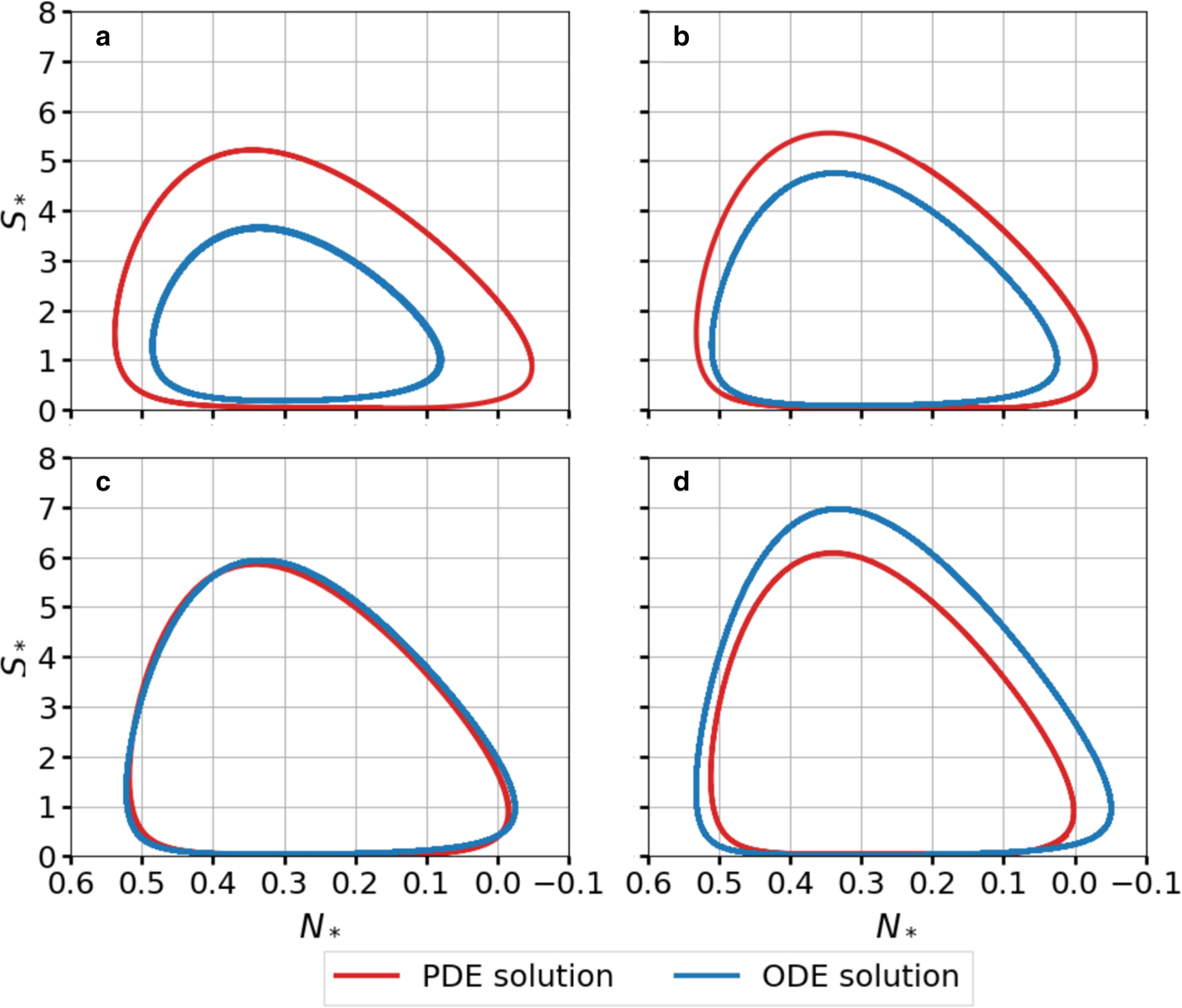
Here we compare the PDE model Eqns (19–26) with the ODE model Eqns (27–31) for a single-lake system. For this comparison, we modify the ODE model to include the function ζ(S) in Eqn (11) that scales the viscous closure rate in the PDE model. This function was neglected in the main text to simplify the bifurcation analysis, but leads to better quantitative agreement with the PDE results. The ODE model includes a parameter ε* > 0 that controls the amplitude and period of the limit cycles. For some optimal ε*, we wish to measure how well the limit cycles from both models agree. In natural systems, the period of the filling–draining cycles is typically the easiest parameter to estimate. Therefore, we define the optimal value of ε* as

where Πp and Πo are the periods of the PDE and ODE solutions, respectively. We note that Πo depends on ε* through solution of Eqns (27–28). With this choice of $\varepsilon _\star$ , the limit cycles from the two models can agree quite well, depending on the choice of a m and a c (Figs 12b–d). However, for small values of a m and a c near the subcritical Hopf bifurcation, the ODE limit cycle has a smaller ampltiude (Fig. 12a).
Limit cycles from the non-dimensional PDE Eqns (19–26) and ODE Eqns (27–31) models. Equation (27) is modified to include the closure rate scale ζ(S) in Eqn (11) with the parameter $S_{\rm f} = 2000 \times \tilde {S}$ . The parameter $\varepsilon_{\ast} = \varepsilon _\star$
 is chosen to minimize the misfit between the periods of the ODE and PDE solutions in Eqn (D1). The parameters for each panel are (a) $(a_{\rm m},\, a_{\rm c},\,\varepsilon _\star )=$
 (10, 136, 0.0252), (b) $(a_{\rm m},\,a_{\rm c},\,\varepsilon _\star )=$
 (12, 164, 0.0282), (c) $(a_{\rm m},\,a_{\rm c},\,\varepsilon _\star )=(14,\,205,\,0.0248)$
 and (d) $(a_{\rm m},\,a_{\rm c},\,\varepsilon _\star ) = (16,\,235,\,0.0201)$
 .
.


 Open access